Primers • Vision Transformer (ViT)
- Overview
- How the Vision Transformer (ViT) works in a nutshell
- ViT v/s CNNs: Data Efficiency and Fine-Tuning
- Representing an image as a sequence of patches
- Positional embeddings
- Key findings
- How far away are the learned non-local interactions?
- Attention distance and visualization
- Implementation
- FAQs
- Why does ViT use linear projections of flattened patches at the input?
- How are linear projections of flattened patches at the input calculated in ViT? What are the inputs and outputs?
- Why does ViT rely on \(16 \times 16\) pixels for its input patches?
- Why does ViT not use a tokenizer at the input (akin to Transformers for text processing tasks)?
- What are “tokens” when embedding an image using an encoder? How are they different compared to word/sub-word tokens in NLP?
- Citation
Overview
-
This article investigates over how the Vision Transformer (ViT) works by going over the minor modifications of the transformer architecture for image classification.
-
We recommend checking out the primers on Transformer and attention prior to exploring ViT.
- Transformers lack the inductive biases of Convolutional Neural Networks (CNNs), such as translation invariance and a locally restricted receptive field. To clarify what this implies: invariance refers to the fact that you can recognize an entity (i.e. object) in an image, even when its appearance or position varies. Translation in computer vision implies that each image pixel has been moved by a fixed amount in a particular direction.
- Moreover, remember that convolution is a linear local operator. We see only the neighbor values as indicated by the kernel.
- On the other hand, the transformer is by design permutation invariant. The bad news is that it cannot process grid-structured data. We need sequences! To this end, we will convert a spatial non-sequential signal to a sequence! Let’s see how.
How the Vision Transformer (ViT) works in a nutshell
-
The total architecture is called Vision Transformer (ViT), proposed by Alexey Dosovitskiy et al. (2020) in An Image is Worth \(16 \times 16\) Words: Transformers for Image Recognition at Scale. Let’s examine it step by step.
- Split an image into patches
- Flatten the patches
- Produce lower-dimensional linear embeddings from the flattened patches
- Add positional embeddings
- Feed the sequence as an input to a standard transformer encoder
- Pretrain the model with image labels (fully supervised on a huge dataset)
- Finetune on the downstream dataset for image classification
-
The following image from Google’s AI blog shows the inner workings of ViT:

- Image patches are basically the sequence tokens (like words). In fact, the encoder block is identical to the original transformer proposed by Vaswani et al. (2017) as we have extensively described. The following image shows the well-known transformer block (source: An Image is Worth \(16 \times 16\) Words: Transformers for Image Recognition at Scale):
![]()
- The only thing that changes is the number of those blocks. To this end, and to further prove that with more data they can train larger ViT variants, 3 models were proposed (source: An Image is Worth \(16 \times 16\) Words: Transformers for Image Recognition at Scale):
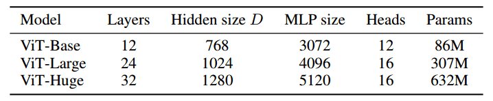
-
Heads refer to multi-head attention, while the MLP size refers to the blue module in the figure. MLP stands for multi-layer perceptron but it’s actually a bunch of linear transformation layers.
-
Hidden size DD is the embedding size, which is kept fixed throughout the layers. Why keep it fixed? So that we can use short residual skip connections.
-
In case you missed it, there is no decoder in the game. Just an extra linear layer for the final classification called MLP head. But is this enough? Yes and no. Actually, we need a massive amount of data and as a result computational resources.
ViT v/s CNNs: Data Efficiency and Fine-Tuning
-
Specifically, if ViT is trained on datasets with more than 14M images it can approach or beat state-of-the-art CNNs. If not, you better stick with ResNets or EfficientNets.
-
ViT is pretrained on the large dataset and then fine-tuned to small ones. The only modification is to discard the prediction head (MLP head) and attach a new \(D \times K\) linear layer, where \(K\) is the number of classes of the small dataset.
It is interesting that the authors claim that it is better to fine-tune at higher resolutions than pre-training.
- To fine-tune in higher resolutions, 2D interpolation of the pre-trained position embeddings is performed. The reason is that they model positional embeddings with trainable linear layers. Having that said, the key engineering part of this paper is all about feeding an image in the transformer.
Representing an image as a sequence of patches
- Let’s go over how you can reshape the image in patches. For an input image \((x) \in R^{H} \times W \times C\) and patch size \(p\), we want to create \(N\) image patches denoted as \((x) p \in R^{N} \times\left(P^{2} C\right)\), where \(N=\frac{H W}{P} \cdot N\) is the sequence length similar to the words of a sentence.
- The image patch, i.e., \([16, 16, 3]\) is flattened to \(16 \times 16 \times 3\). The title of the paper should now make sense :)
- Let’s use the
einopslibrary that works atop PyTorch. You can install it viapip:
$ pip install einops
- And then some compact Pytorch code:
from einops import rearrange

p = patch_size # P in maths

x_p = rearrange(img, 'b c (h p1) (w p2) -> b (h w) (p1 p2 c)', p1 = p, p2 = p)
- In short, each symbol or each parenthesis indicates a dimension. For more information on einsum operations check out this blogpost on einsum operations.
- Note that the image patches are always squares for simplicity.
- And what about going from patch to embeddings? It’s just a linear transformation layer that takes a sequence of \(P^{2} C\) elements and outputs \(D\).
patch_dim = (patch_size**2) * channels # D in math

patch_to_embedding = nn.Linear(patch_dim, dim)
- What’s missing is that we need to provide some sort of order.
Positional embeddings
- Even though many positional embedding schemes were applied, no significant difference was found. This is probably due to the fact that the transformer encoder operates on a patch-level. Learning embeddings that capture the order relationships between patches (spatial information) is not so crucial. It is relatively easier to understand the relationships between patches of \(P \times P\) than of a full image \(Height \times Width\).
Intuitively, you can imagine solving a puzzle of 100 pieces (patches) compared to 5000 pieces (pixels).
- Hence, after the low-dimensional linear projection, a trainable position embedding is added to the patch representations. It is interesting to see what these position embeddings look like after training (source: An Image is Worth \(16 \times 16\) Words: Transformers for Image Recognition at Scale):
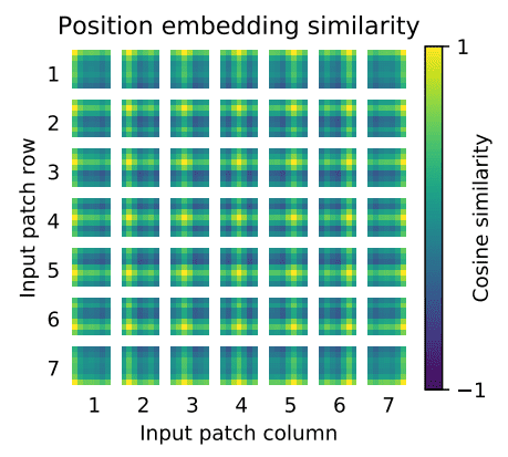
- First, there is some kind of 2D structure. Second, patterns across rows (and columns) have similar representations. For high resolutions, a sinusoidal structure was used.
Key findings
- In the early CNN days, we used to visualize the early layers. Why? Because we believe that well-trained networks often show nice and smooth filters. This following image visualizes AlexNet’s learned filters on the left (source: Standford’s Course CS231n and ViT’s learned filters on the right (source: An Image is Worth \(16 \times 16\) Words: Transformers for Image Recognition at Scale).
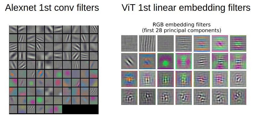
- As stated in CS231n:
“Notice that the first-layer weights are very nice and smooth, indicating a nicely converged network. The color/grayscale features are clustered because the AlexNet contains two separate streams of processing, and an apparent consequence of this architecture is that one stream develops high-frequency grayscale features and the other low-frequency color features.” ~ Stanford CS231 Course: Visualizing what ConvNets learn
- For such visualizations PCA is used. In this way, the author showed that early layer representations may share similar features.
How far away are the learned non-local interactions?
-
Short answer: For patch size \(P\), maximum \(P \times P\), which in our case is 128, even from the 1st layer!
-
We don’t need successive Conv layers to get to 128-away pixels anymore. With convolutions without dilation, the receptive field is increased linearly. Using self-attention we have interaction between pixels representations in the 1st layer and pairs of representations in the 2nd layer and so on. The following image shows the mean attention distance v/s the network depth (source: An Image is Worth \(16 \times 16\) Words: Transformers for Image Recognition at Scale) the receptive field growth on the right (source: generated using Fomoro AI calculator).
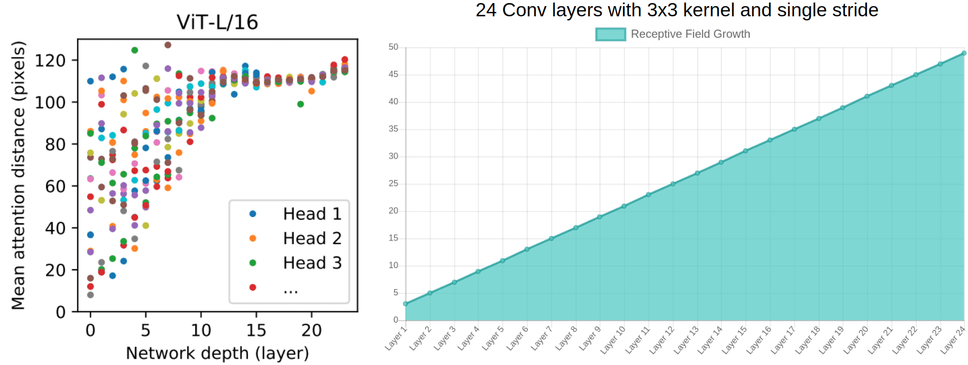
- Based on the diagram on the left from ViT, one can argue that:
- There are indeed heads that attend to the whole patch already in the early layers.
- One can justify the performance gain based on the early access pixel interactions. It seems more critical for the early layers to have access to the whole patch (global info). In other words, the heads that belong to the upper left part of the image may be the core reason for superior performance.
- Interestingly, the attention distance increases with network depth similar to the receptive field of local operations.
- There are also attention heads with consistently small attention distances in the low layers. On the right, a 24-layer with standard 3x3 convolutions has a receptive field of less than 50. We would approximately need 50 conv layers, to attend to a ~100 receptive field, without dilation or pooling layers.
- To enforce this idea of highly localized attention heads, the authors experimented with hybrid models that apply a ResNet before the Transformer. They found less highly localized heads, as expected. Along with filter visualization, it suggests that it may serve a similar function as early convolutional layers in CNNs.
Attention distance and visualization
- It is critical to understand how they measured the mean attention distance. It’s analogous to the receptive field, but not exactly the same.
- Attention distance was computed as the average distance between the query pixel and the rest of the patch, multiplied by the attention weight. They used 128 example images and averaged their results.
- An example: if a pixel is 20 pixels away and the attention weight is 0.5 the distance is 10.
- Finally, the model attends to image regions that are semantically relevant for classification, as illustrated below (source: An Image is Worth \(16 \times 16\) Words: Transformers for Image Recognition at Scale):

Implementation
-
The following implementation demonstrates a minimal ViT model, leveraging a pre-existing vanilla Transformer encoder architecture. The primary operations in this model include:
- Dividing the input image into non-overlapping patches.
- Flattening each patch into a vector.
- Projecting these flattened vectors into a fixed-dimensional embedding space using a fully connected linear layer.
- Adding learnable positional embeddings to preserve spatial information.
- Processing the sequence of patch embeddings through a Transformer encoder.
- Optionally utilizing a classification token for downstream tasks such as image classification.
-
This design adheres to the fundamental ViT principles while maintaining flexibility for customization, such as varying patch sizes, embedding dimensions, and the number of Transformer blocks.
import torch
import torch.nn as nn
from einops import rearrange

from self_attention_cv import TransformerEncoder


class ViT(nn.Module):
    def __init__(self, *,
                 img_dim,
                 in_channels=3,
                 patch_dim=16,
                 num_classes=10,
                 dim=512,
                 blocks=6,
                 heads=4,
                 dim_linear_block=1024,
                 dim_head=None,
                 dropout=0, transformer=None, classification=True):
        """
        Args:
            img_dim: the spatial image size
            in_channels: number of img channels
            patch_dim: desired patch dim
            num_classes: classification task classes
            dim: the linear layer's dim to project the patches for MHSA
            blocks: number of transformer blocks
            heads: number of heads
            dim_linear_block: inner dim of the transformer linear block
            dim_head: dim head in case you want to define it. defaults to dim/heads
            dropout: for pos emb and transformer
            transformer: in case you want to provide another transformer implementation
            classification: creates an extra CLS token
        """
        super().__init__()
        assert img_dim % patch_dim == 0, f'patch size {patch_dim} not divisible'
        self.p = patch_dim
        self.classification = classification
        tokens = (img_dim // patch_dim) ** 2
        self.token_dim = in_channels * (patch_dim ** 2)
        self.dim = dim
        self.dim_head = (int(dim / heads)) if dim_head is None else dim_head
        self.project_patches = nn.Linear(self.token_dim, dim)

        self.emb_dropout = nn.Dropout(dropout)
        if self.classification:
            self.cls_token = nn.Parameter(torch.randn(1, 1, dim))
            self.pos_emb1D = nn.Parameter(torch.randn(tokens + 1, dim))
            self.mlp_head = nn.Linear(dim, num_classes)
        else:
            self.pos_emb1D = nn.Parameter(torch.randn(tokens, dim))

        if transformer is None:
            self.transformer = TransformerEncoder(dim, blocks=blocks, heads=heads,
                                                  dim_head=self.dim_head,
                                                  dim_linear_block=dim_linear_block,
                                                  dropout=dropout)
        else:
            self.transformer = transformer

    def expand_cls_to_batch(self, batch):
        """
        Args:
            batch: batch size
        Returns: cls token expanded to the batch size
        """
        return self.cls_token.expand([batch, -1, -1])

    def forward(self, img, mask=None):
        batch_size = img.shape[0]
        img_patches = rearrange(
            img, 'b c (patch_x x) (patch_y y) -> b (x y) (patch_x patch_y c)',
                                patch_x=self.p, patch_y=self.p)
        # project patches with linear layer + add pos emb
        img_patches = self.project_patches(img_patches)

        if self.classification:
            img_patches = torch.cat(
                (self.expand_cls_to_batch(batch_size), img_patches), dim=1)

        patch_embeddings = self.emb_dropout(img_patches + self.pos_emb1D)

        # feed patch_embeddings and output of transformer. shape: [batch, tokens, dim]
        y = self.transformer(patch_embeddings, mask)

        if self.classification:
            # we index only the cls token for classification. nlp tricks :P
            return self.mlp_head(y[:, 0, :])
        else:
            return y
Code Explanation
-
In this implementation:
- The
rearrangefunction fromeinopsreshapes the input tensor into a sequence of flattened image patches. Each patch is of shape \(P^2 C\), where \(P\) is the patch size and \(C\) is the number of image channels. - The
nn.Linearlayer (self.project_patches) acts as the learnable fully connected projection, mapping each flattened patch to a \(D\)-dimensional embedding vector. This corresponds to the initial linear projection stage in ViT. - A learnable classification token (
cls_token) is optionally prepended to the patch sequence whenclassification=True. - Learnable positional embeddings (
pos_emb1D) are added to each token to encode spatial information. - The resulting sequence is processed by a Transformer encoder, which models global dependencies between patches.
- For classification tasks, only the output corresponding to the classification token is passed through a final linear layer (
mlp_head) to produce class logits. For non-classification tasks, the output embeddings for all tokens are returned.
- The
-
This structure provides a clean and modular ViT design while retaining flexibility for experimentation with architectural parameters.
Conv2D Equivalence for Patch Projection
-
Although this code uses
nn.Linearfor patch projection, such as the official Google ViT code and timm’sPatchEmbedmodule replace it with ann.Conv2dlayer, where:- Kernel size = patch size (\(P\))
- Stride = patch size (\(P\))
- Input channels = \(C\) (number of image channels)
- Output channels = \(D\) (embedding dimension)
-
This convolution operation directly extracts and projects patches without explicit flattening. It is mathematically equivalent to the linear projection in this implementation, but it is more efficient on GPUs due to optimized convolution kernels.
FAQs
Why does ViT use linear projections of flattened patches at the input?
-
The ViT model uses linear projections of flattened patches at the input for several reasons:
-
Reduction of Dimensionality: Images are inherently high-dimensional data. Flattening and projecting the patches into a lower-dimensional space makes the computation more manageable and efficient. This process is analogous to reducing the resolution of an image while retaining essential features.
-
Uniform Data Representation: By flattening and projecting, the vision transformer treats the image patches similarly to how tokens (words) are treated in a language model. This uniformity allows the use of transformer architecture, originally designed for NLP tasks, in processing visual data.
-
Capturing Local Features: Each patch represents local features of the image. By projecting these patches, the model can capture and process these local features effectively. This is akin to how convolutional neural networks (CNNs) operate, but with a different approach.
-
Scalability and Flexibility: The approach allows the model to be scalable to different image sizes and resolutions. It also offers flexibility in terms of the size of the patches and the depth of the network.
-
Enabling Positional Encoding: Flattening and projecting the patches allow for the addition of positional encodings. In transformers, positional encodings are crucial as they provide the model with information about the relative or absolute position of the patches in the image. Unlike CNNs, transformers do not inherently understand the order or position of the input data, so positional encodings are necessary.
-
Facilitating Self-Attention Mechanism: The transformer architecture relies heavily on the self-attention mechanism, which computes the response at a position in a sequence (in this case, a sequence of patches) by attending to all positions and computing a weighted sum of their features. Flattened and projected patches are conducive to this mechanism.
-
-
In summary, the use of linear projections of flattened patches in ViT is a strategic design choice that leverages the strengths of transformer architecture while making it suitable for processing visual data. This method allows the model to handle high-dimensional image data efficiently, capture local features, and utilize the self-attention mechanism effectively.
How are linear projections of flattened patches at the input calculated in ViT? What are the inputs and outputs?
-
In ViT, the linear projections of flattened patches at the input are performed using a learnable fully connected (linear) layer. This is the very first step in transforming an image into a sequence of embeddings that can be processed by a transformer. Let’s break down the steps, inputs, and outputs:
-
Input Image Processing:
- Input: The input is a raw image of size \(H \times W \times C\) (height, width, channels).
- Patching: The image is divided into non-overlapping patches of size \(P \times P\). For example, if \(P = 16\), each patch is \(16 \times 16\) pixels.
- Flattening: Each patch is flattened into a 1D vector. If a patch is \(16 \times 16\) pixels with 3 color channels (RGB), each flattened patch has \(16 \times 16 \times 3 = 768\) elements.
-
Linear Projection via Fully Connected Layer:
- Flattened Patches: The flattened patch vectors from the previous step are the inputs to the projection stage.
- Fully Connected Layer: This stage is implemented as a standard Linear (fully connected) layer without any non-linearity, with weight matrix \(W \in \mathbb{R}^{D \times (P^2 C)}\) and bias vector \(b \in \mathbb{R}^D\), where \(D\) is the embedding dimension. This projection is a Linear layer without a non-linearity (just an affine transform).
-
Calculation: For each patch vector \(x_p\), the embedding is computed as:
\[z_p = W x_p + b\]This transforms each \(P^2 C\)-dimensional flattened patch into a \(D\)-dimensional patch embedding.
- Efficiency Note: Some implementations replace the explicit flattening and linear layer with a
Conv2Doperation havingkernel size = patch sizeandstride = patch size, which is mathematically equivalent to the linear projection, but more efficient on GPUs.
-
Addition of Positional Encodings:
- Positional Embeddings: Learnable positional embeddings are added to each patch embedding to retain spatial information about where the patch came from in the original image.
- Final Patch Representation: Each patch embedding is summed with its positional embedding to form the final patch representation.
-
Sequence Formation for Transformer:
- Sequence of Patch Representations: The sequence of final patch representations, each of size \(D\), is fed into the transformer encoder for further processing.
-
-
In summary:
- Inputs: A raw image, split into patches and flattened.
- Process: Each flattened patch is projected into a \(D\)-dimensional embedding using a fully connected linear layer (or equivalent
Conv2D), followed by the addition of positional encodings. - Outputs: A sequence of patch embeddings with positional information, ready for transformer processing.
-
This process adapts the transformer’s text-oriented architecture to handle images by representing the image as a sequence of learned embeddings, much like word embeddings in NLP.
Why does ViT rely on \(16 \times 16\) pixels for its input patches?
-
ViT often uses \(16 \times 16\) pixel patches for its input, but this choice is not a strict requirement; it’s more of a practical and empirical decision. Let’s explore why \(16 \times 16\) is commonly used and whether other patch sizes could work:
-
Balance Between Granularity and Computational Efficiency: A \(16 \times 16\) patch size is a compromise between capturing sufficient detail in each patch and keeping the number of patches (and thus the sequence length for the transformer) manageable. Smaller patches would provide more detailed information but would increase the sequence length and computational cost. Larger patches would reduce the sequence length but might miss finer details in the image.
-
Empirical Performance: The choice of \(16 \times 16\) has been empirically found to work well for a range of tasks and datasets in many studies and applications. This practical experience has led to its common adoption.
-
Comparison with Convolutional Networks: The patch size somewhat mirrors the receptive field of filters in traditional convolutional neural networks (CNNs). In CNNs, filters capture local patterns, and their effective receptive field often aligns with the size of these patches in ViTs.
-
Hardware and Memory Constraints: The patch size also needs to be chosen considering the hardware and memory constraints. Larger models with smaller patches might not be feasible for training and inference on available hardware.
-
Other Patch Sizes: ViTs can certainly work with other patch sizes. The choice of patch size is a hyperparameter that can be tuned based on the specific requirements of the task, the nature of the dataset, and the available computational resources. For instance, for higher resolution images or tasks requiring finer details, smaller patches might be more suitable. Conversely, for tasks where global features are more important, larger patches could be used.
-
-
In summary, while \(16 \times 16\) pixels is a common choice for input patches in ViTs due to a balance between detail capture and computational efficiency, it is not a fixed requirement. Other patch sizes can be used, and the optimal choice depends on the specific task, dataset characteristics, and available computational resources. Experimentation and empirical validation are key in determining the most suitable patch size for a given application.
Why does ViT not use a tokenizer at the input (akin to Transformers for text processing tasks)?
-
In ViTs, the concept of tokenization is applied differently compared to how it’s used in traditional text-based transformers. ViTs do not use a tokenizer in the same sense as NLP models, and here’s why:
-
Nature of Input Data: In NLP, tokenization is used to convert text into a series of tokens (words or subwords), which are then mapped to embeddings. This is necessary because text data is discrete and symbolic. In contrast, images are continuous and high-dimensional. The concept of ‘words’ or ‘characters’ does not directly apply to images.
-
Image Patching as a Form of Tokenization: In ViTs, the closest analog to tokenization is the division of an image into fixed-size patches. Each patch is treated as a ‘token’. These patches are then flattened and linearly projected into embeddings. This process can be thought of as a form of tokenization where each ‘token’ represents a part of the image rather than a word or character.
-
Absence of Vocabulary: In text processing, tokenization is followed by mapping tokens to a vocabulary of known words or subwords. For images, there is no predefined vocabulary. Each patch is unique and is represented by its pixel values, which are then projected into a latent space.
-
Direct Processing of Raw Input: Unlike text, where tokenization is a necessary preprocessing step to handle the symbolic nature of language, ViTs can process raw image data directly (after patching and embedding). This direct processing of visual information is more analogous to how convolutional neural networks (CNNs) handle images, although the mechanisms are different.
-
-
In summary, while ViTs don’t use a tokenizer in the traditional NLP sense, the process of dividing an image into patches and linearly projecting these patches serves a similar purpose. It converts the raw image data into a format that can be processed by the transformer architecture, ensuring that spatial information is retained and managed efficiently. The key difference lies in the nature of the input data and how it’s represented and processed within the model.
What are “tokens” when embedding an image using an encoder? How are they different compared to word/sub-word tokens in NLP?
- When embedding an image using an encoder in the context of machine learning and neural networks, there are indeed “tokens,” although they might not be tokens in the traditional sense as understood in natural language processing (NLP).
- In NLP, tokens usually refer to words or subwords. However, in the context of image processing, an encoder, especially in models like ViT, converts an image into a series of numerical representations, which can be analogously thought of as “tokens.”
-
Here’s a simplified breakdown of the process:
-
Image Segmentation: The image is divided into patches. Each patch can be seen as a visual “word.” This is analogous to tokenization in NLP, where a sentence is broken down into words or subwords.
-
Flattening and Linear Projection: Each patch is then flattened (turned into a 1D array) and passed through a linear projection to obtain a fixed-size vector. These vectors are the equivalent of word embeddings in NLP.
-
Sequence of Embeddings: The sequence of these vectors (one for each patch) is what the Transformer encoder processes. Each vector represents the “token” corresponding to a part of the image.
-
Positional Encoding: Since Transformers don’t have a sense of order, positional encodings are added to these embeddings to provide information about the location of each patch in the image.
-
Transformer Encoder: The sequence of patch embeddings, now with positional information, is fed into the Transformer encoder. The encoder processes these embeddings (tokens) through its layers, enabling the model to understand and encode complex relationships and features within the image.
-
- In summary, while the term “tokens” originates from text processing, its use in image processing with encoders like ViT is an analogy to how images are broken down into manageable, meaningful segments for the model to process, similar to how text is tokenized into words or subwords.
Citation
If you found our work useful, please cite it as:
@article{Chadha2020DistilledVisionLanguageModels,
  title   = {Vision Language Models},
  author  = {Chadha, Aman},
  journal = {Distilled AI},
  year    = {2020},
  note    = {\url{https://aman.ai}}
}