Primers • Receptive Field
- Introduction
- What is the receptive field in deep learning?
- Why do we care about the receptive field of a convolutional network?
- Closed-form calculations of the receptive field for single-path networks
- How can we increase the receptive field in a convolutional network?
- Understanding the effective receptive field
- Conclusion
- Further Reading
- References
- Citation
Introduction
-
In this article, we will discuss multiple perspectives that involve the receptive field of a deep convolutional architecture. We will address the influence of the receptive field starting for the human visual system. As you will see, a lot of terminology of deep learning comes from neuroscience. As a short motivation, convolutions are awesome but it is not enough just to understand how it works. The idea of the receptive field will help you dive into the architecture that you are using or developing. This article offers an in-depth analysis to understand how you can calculate the receptive field of your model as well as the most effective ways to increase it.
-
According to the “Receptive field” article on Wikipedia, the receptive field (of a biological neuron) is “the portion of the sensory space that can elicit neuronal responses, when stimulated”. The sensory space can be defined in any dimension (e.g. a 2D perceived image for an eye). Simply, the neuronal response can be defined as the firing rate (i.e., number of action potentials generated by a neuron). It is related to the time dimension based on the stimuli. What is important is that it affects the received frames per second (FPS) of our visual system. It is not clear what is the exact FPS of our visual system, and it is definitely changing in different situations (i.e., when we are in danger). The “Frame rate: Human Vision” article on Wikipedia says:
Insight: The human visual system can process 10 to 12 images per second and perceive them individually, while higher rates are perceived as motion.
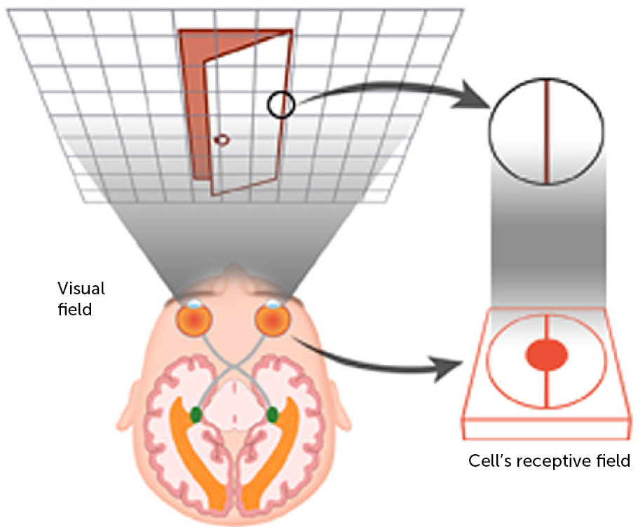
- Let’s observe the visual human system (image taken from brainconnection) to further clarify these concepts:
-
Based on the image, the entire area (in this case, the grid in the figure) an eye can see is called the field of view. The human visual system consists of millions of neurons, where each one captures different information. We define the neuron’s receptive field as the patch of the total field of view – in other words, the information a single neuron has access to. This is in simple terms the biological cell’s receptive field.
-
Now, let’s see how we can extend this idea to convolutional networks.
What is the receptive field in deep learning?
- Per Araujo et al., in a deep learning context, the Receptive Field (RF) is defined as the size of the region in the input that produces the feature. Basically, it is a measure of association of an output feature (of any layer) to the input region (patch), i.e., the “perspective” of the model when generating the output feature. Before we move on, let’s clarify one important thing:
Insight: The idea of receptive fields applies to local operations (i.e., convolution, pooling).
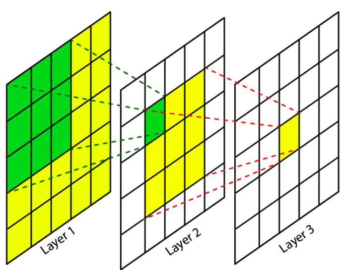
- The following image from Research Gate shows the receptive field of three successive conv layers:
-
A convolutional unit only depends on a local region (patch) of the input. That’s why we never refer to the RF on fully connected layers since each unit has access to all the input region. To this end, the aim of this article is to develop intuition about this concept, in order to understand and analyze how deep convolutional networks with local operations work.
-
Ok, but why should anyone care about the RF?
Why do we care about the receptive field of a convolutional network?
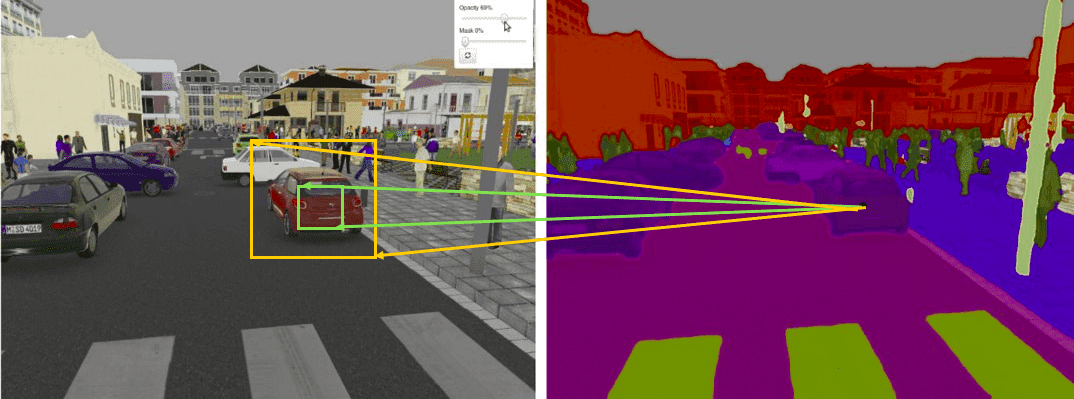
- There is no better way to clarify this than a couple of computer vision examples. In particular, let’s revisit a couple of dense prediction computer vision tasks. Specifically, in image segmentation and optical flow estimation, we produce a prediction for each pixel in the input image, which corresponds to a new image, the semantic label map. Ideally, we would like each output pixel of the label map to have a big receptive field, so as to ensure that no crucial information was not taken into account. For instance, if we want to predict the boundaries of an object (i.e., a car, an organ like the heart, a tumor) it is important that we provide the model access to all the relevant parts of the input object that we want to segment. In the image below (from Nvidia’s blog), you can see two receptive fields: the green and the orange one. Which one would you prefer?
-
Similarly, in object detection, a small receptive field may not be able to recognize large objects. That’s why you usually see multi-scale approaches in object detection. Furthermore, in motion-based tasks, like video prediction and optical flow estimation, we want to capture large motions (displacements of pixels in a 2D grid), so we want to have an adequate receptive field. Specifically, the receptive field should be sufficient if it is larger than the largest flow magnitude of the dataset.
-
Therefore, our goal is to design a convolutional model so that we ensure that its RF covers the entire relevant input image region.
-
In the diagram below (borrowed from Araujo et al.), you can see the relation of the RF to the classification accuracy in ImageNet. The radius refers to the amount of floating-point operations (FLOPs) of each model. The purple corresponds to the ResNet family (50-layer, 101, and 152 layers), while the yellow is the Inception family (v2, v3, v4). Light-blue is the MobileNet architecture.
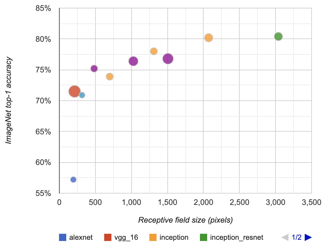
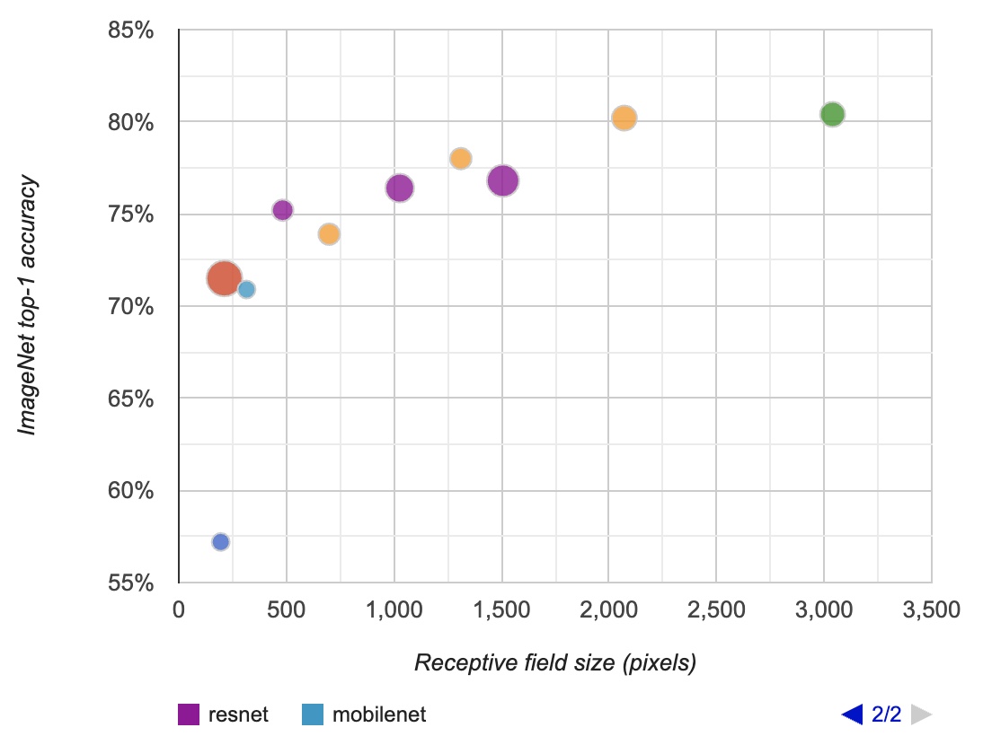
- As described in “Computing receptive fields of convolutional neural networks” by Araujo et al. (2019):
“We observe a logarithmic relationship between classification accuracy and receptive field size, which suggests that large receptive fields are necessary for high-level recognition tasks, but with diminishing rewards.”
-
Nevertheless, the receptive field size alone is not the only factor contributing to improved recognition performance. However, the point is that you should definitely be aware of your model’s receptive field.
-
Ok, so how can we measure it?
Closed-form calculations of the receptive field for single-path networks
-
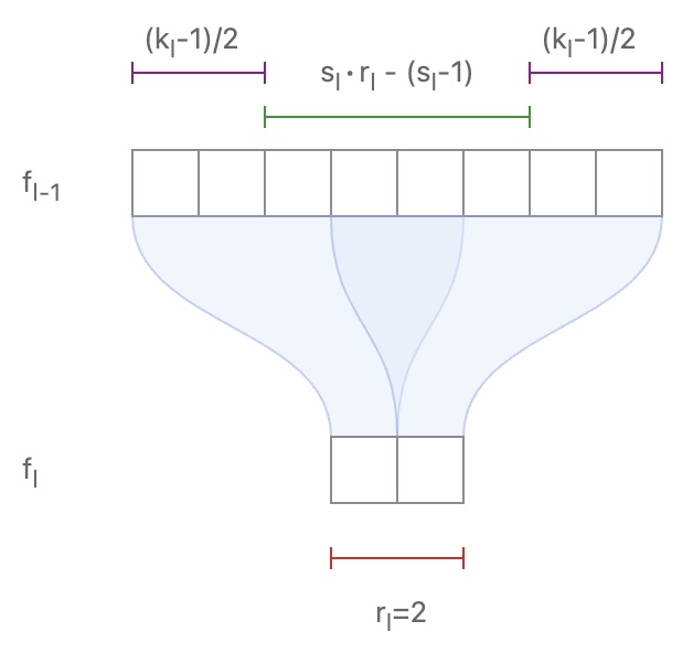
Araujo et al. (2019) provide an intuitive way to calculate in an analytical form the RF of your model. A single path literally means no skip connections in the architecture, like the famous AlexNet. Let’s see some math! For two sequential convolutional layers \(f_2\), \(f_1\) with kernel size \(k\), stride \(s\), receptive field \(r\):
\[r_1 = s_2 \times r_2 + (k_2-s_2)\]- Or in a more general form:
-
The image below may help you clarify this equation. Note that we are interested to see the influence of the receptive field starting from the last layer towards the input. So, in that sense, we go backwards. The following diagram (taken from Araujo et al. (2019)) visualizes 1D sequential conv:
-
It seems like this equation can be generalized to a beautiful compact form that simply applies this operation recursively for \(L\) layers. By further analyzing the recursive equation, we can derive a closed form solution that depends only on the convolutional parameters of kernels and strides:
\[r_0 = \sum_{i=1}^{L} ( (k_{i} -1) \prod_{j=1}^{l-1} s_{j} ) + 1 \tag{1}\]- where \(r_0\) denotes the desired RF of the architecture.
-
Now the next question is… Now that we have measured the theoretical RF of our model, how do we increase it?
How can we increase the receptive field in a convolutional network?
-
In essence, there are a plethora of ways and tricks to increase the RF, that can be summarized as follows:
-
Add more convolutional layers (make the network deeper)
-
Add pooling layers or higher stride convolutions (sub-sampling)
-
Depth-wise convolutions
-
-
Let’s look at the distinct characteristics of these approaches.
Add more convolutional layers
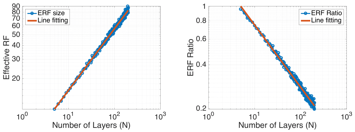
- Per “Understanding the effective receptive field in deep convolutional neural networks” by Luo et al. (2016), adding more convolutional layers increases the receptive field size linearly, as each extra layer increases the receptive field size by the kernel size. Moreover, it is experimentally validated that as the theoretical receptive field is increasing but the effective (experimental) receptive field (ERF) is reducing. The following figure (taken from Luo et al. (2016)) shows the impact of increasing the number of layers decreases the ERF ration:
Sub-sampling and dilated convolutions
-
Sub-sampling techniques like pooling on the other hand, increases the receptive field size multiplicatively. Modern architectures like ResNet combine adding more convolutional layers and sub-sampling. On the other hand, sequentially placed dilated convolutions, increase the RF exponentially.
-
But first, let’s revisit the idea of dilated convolutions.
-
In essence, dilated convolutions introduce another parameter, denoted as \(r\), called the dilation rate. Dilations introduce “holes” in a convolutional kernel. The “holes” basically define a spacing between the values of the kernel. So, while the number of weights in the kernel is unchanged, the weights are no longer applied to spatially adjacent samples. Dilating a kernel by a factor of \(r\) introduces a kind of striding of \(r\).
-
The equation \((1)\) in the above section can be reused by simply replacing the kernel size \(k\) for all layers using dilations:
- All the above can be illustrated in the following animation, from “A guide to convolutional arithmetic” by Dumoulin (2016).
-
Now, let’s briefly inspect how dilated convolutions can influence the receptive field.
-
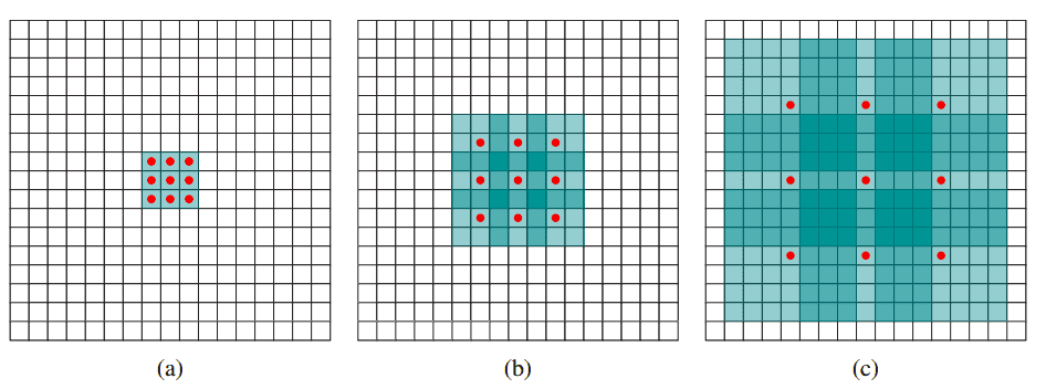
Let’s dig into three sequential conv. Layers (denoted by \(a, b, c\)) that are illustrated in the image with normal convolution, \(r = 2\) dilation factor, and \(r = 4\) dilation factor. We will intuitively understand why dilation supports an exponential expansion of the receptive field without loss of resolution (i.e., pooling) or coverage. Refer to the following image from “Multi-scale context aggregation by dilated convolutions” by Yu and Koltun (2015):
Analysis
- In (a), we have a normal \(3 \times 3\) convolution with receptive field \(3 \times 3\).
- In (b), we have a 2-dilated \(3 \times 3\) convolution that is applied in the output of layer (a) which is a normal convolution. As a result, each element in the 2 coupled layers now has a receptive field of \(7 \times 7\). If we studied 2-dilated conv alone the receptive field would be simply \(5 \times 5\) with the same number of parameters.
-
In (c), by applying a 4-dilated convolution, each element in the third sequential conv layer now has a receptive field of \(15 \times 15\). As a result, the receptive field grows exponentially while the number of parameters grows linearly per Yu and Koltun (2015).
- In other words, a \(3 \times 3\) kernel with a dilation rate of 2 will have the same receptive field as a \(5 \times 5\) kernel, while only using 9 parameters. Similarly, a \(3 \times 3\) kernel with a dilation rate of 4 will have the same receptive field as a \(9 \times 9\) kernel without dilation. Mathematically:
Insight: In deep architectures, we often introduce dilated convolutions in the last convolutional layers.
- Below you can observe the resulting ERF (effective receptive field) when introducing pooling and dilation in an experimental study performed by Luo et al. (2016). The receptive field is larger in both cases than the vanilla conv, but is largest with pooling. We’ll see more about the effective receptive field in a later section. The following figure (taken from Luo et al. (2016)) shows a visualization of the effective receptive field (ERF) by introducing pooling strategies and dilation:
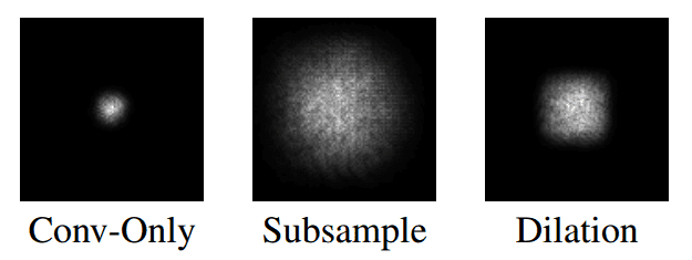
Insight: Based on Luo et al. (2016), pooling operations and dilated convolutions turn out to be effective ways to increase the receptive field size quickly.
Depth-wise convolutions
- Finally as described in “Computing receptive fields of convolutional neural networks” by Araujo et al. (2019), with depth-wise convolutions the receptive field is increased with a small compute footprint, so it is considered a compact way to increase the receptive field with fewer parameters. Depthwise convolution is the channel-wise spatial convolution. However, note that depth-wise convolutions do not directly increase the receptive field. But since we use fewer parameters with more compact computations, we can add more layers. Thus, with roughly the same number of parameters, we can get a bigger receptive field. MobileNet by Howard et al. (2017) achieves high recognition performance based on this idea.
Skip-connections and receptive field
-
If you want to revisit the intuition behind skip connections, check out our article on Skip Connections.
-
In a model without any skip-connections, the receptive field is considered fixed. However, when introducing \(n\) skip-residual blocks, the networks utilize \(2^n\) different paths and therefore features can be learned with a large range of different receptive fields by Li et al. (2017). For example, the HighResNet architecture has a maximum receptive field of 87 pixels, coming from 29 unique paths. In the following figure, we can observe the distribution of the receptive field of these paths in the architecture. The receptive field, in this case, ranges from 3 to 87, following a binomial distribution. The histogram of receptive field distribution from “On the compactness, efficiency, and representation of 3D convolutional networks: brain parcellation as a pretext task” by Li et al. (2017) is as follows:
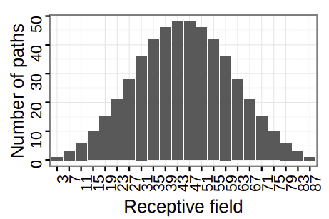
Insight: Skip-connections may provide more paths, however, based on Luo et al. (2016), they tend to make the effective receptive field smaller.
Receptive field and transposed convolutions, upsampling, separable convolutions, and batch normalization
Upsampling
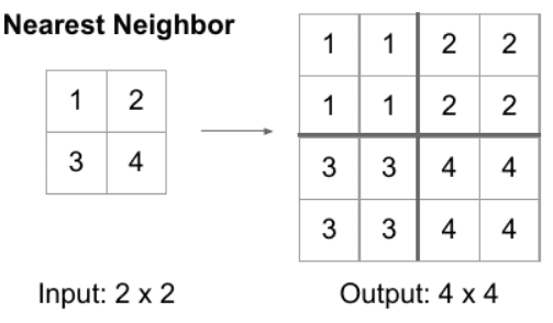
- Upsampling is also a local operation. For the purposes of RF computation, we can consider the kernel size to be equal to the number of input features involved in the computation of an output feature. Since we usually double the spatial dimension, as shown in the figure below, the kernel is \(k=1\).
Separable convolutions
- In short, the RF properties of the separable convolution are identical to its corresponding equivalent non-separable convolution. So, practically nothing changes in terms of the receptive field.
Batch normalization
- During training, batch normalization parameters are computed based on all the channel elements of the feature map. Thus, one can state that its receptive field is the whole input image.
Understanding the effective receptive field
-
In “Understanding the effective receptive field in deep convolutional neural networks” by Luo et al. (2016) discover that not all pixels in a receptive field contribute equally to an output unit’s response. In the previous image, we observed that the receptive field varies with skip connections.
-
Obviously, the output feature is not equally impacted by all pixels within its receptive field. Intuitively, it is easy to perceive that pixels at the center of a receptive field have a much larger impact on output since they have more “paths” to contribute to the output.
-
As a natural consequence, one can define the relative importance of each input pixel as the effective receptive field (ERF) of the feature. In other words, ERF defines the effective receptive field of a central output unit as the region that contains any input pixel with a non-negligible impact on that unit.
-
Specifically, as it is referenced in Luo et al. (2016) we can intuitively realize the contribution of central pixels in the forward and backward pass as:
“In the forward pass, central pixels can propagate information to the output through many different paths, while the pixels in the outer area of the receptive field have very few paths to propagate its impact. In the backward pass, gradients from an output unit are propagated across all the paths, and therefore the central pixels have a much larger magnitude for the gradient from that output.” - by Luo et al. (2016).
- A natural way to measure this impact is of course the partial derivative, rate of change of the unit with respect to the input, as it is computed by backpropagation.
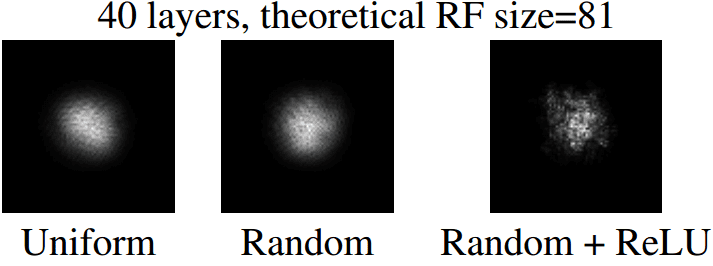
-
As illustrated in the figure above, the ERF is a perfect example of a textbook 2D Gaussian distribution. However, when we add non-linearities, we force the distribution to deviate from a perfect Gaussian. In simple terms, when the pixel-value is zeroed with the ReLU, no path from the receptive field can reach the output, hence the gradient is zero.
-
Based on this study the main insight is the following:
Insight: The ERF in deep convolutional networks actually grows a lot slower than we calculate in theory - by Luo et al. (2016).
- Last but not least, it is super important to highlight that after the training process the ERF is increased, minimizing the gap between the theoretical RF and the ERF before training.
Conclusion
-
In this article, we inspected several aspects of the concept of the Receptive Field. We drew parallels with the human visual system and the concept of RF in CNNs. We discussed the closed-form math, skip connections in RF, and how you can increase it efficiently. Based on that, you can implement the referenced design choices in your model, while being aware of its implications.
-
Key takeaways:
- The idea of receptive fields applies to local operations.
- We want to design a model so that it’s receptive field covers the entire relevant input image region.
- Adding more convolutional layers increases the receptive field size linearly, as each extra layer increases the receptive field size by the kernel size.
- By using sequential dilated convolutions the receptive field grows exponentially, while the number of parameters grows linearly.
- Pooling operations and dilated convolutions turn out to be effective ways to increase the receptive field size quickly.
- Skip-connections may provide more paths, but tend to make the effective receptive field smaller.
- The effective receptive field is increased after training.
-
As a final note, the understanding of RF in convolutional neural networks is an open research topic that will provide a lot of insights on what makes deep convolutional networks tick.
Further Reading
- Here are some (optional) links you may find interesting:
- Understanding the Effective Receptive Field in Deep Convolutional Neural Networks by Luo et al. (2016)
- As an additional resource on the interpretation and visualization of RF, check out “Interpretation of ResNet by Visualization of Preferred Stimulus in Receptive Fields” by Kobayashi et al. (2020). For our more practical reader, if you want a toolkit to automatically measure the receptive field of your model in PyTorch in TensorFlow, we got your back. Finally, for those of you who are hungry for knowledge and curious for bio-inspired concepts like me, especially about the human visual system, you can watch this highly recommended starting video:
References
-
Receptive field on Wikipedia
-
Frame rate: Human Vision on Wikipedia
-
The effective receptive field on CNNs by Christian Perone
-
Understanding the receptive field of deep convolutional networks by Nikolas Adaloglou
-
Computing receptive fields of convolutional neural networks by Araujo et al. (2019)
-
Deep residual learning for image recognition by He et al. (2016)
-
Rethinking the inception architecture for computer vision by Szegedy et al. (2016)
-
Understanding the Effective Receptive Field in Deep Convolutional Neural Networks by Luo et al. (2016)
-
On the compactness, efficiency, and representation of 3D convolutional networks: brain parcellation as a - ext task by Li et al. (2017)
-
Multi-scale context aggregation by dilated convolutions by Yu and Koltun (2015)
-
MobileNets: Efficient convolutional neural networks for mobile vision applications by Howard et al. (2017)
-
A guide to convolution arithmetic for deep learning by Dumoulin and Visin (2016).
-
Interpretation of ResNet by Visualization of Preferred Stimulus in Receptive Fields by Kobayashi and Shouno (2020).
Citation
If you found our work useful, please cite it as:
@article{Chadha2020DistilledReceptiveField,
  title   = {Receptive Field},
  author  = {Chadha, Aman},
  journal = {Distilled AI},
  year    = {2020},
  note    = {\url{https://aman.ai}}
}