Natural Language Processing • Attention
- Overview
- Origins of attention
- Attention: Under the hood
- The Classic Sequence-to-Sequence Model
- Sequence-to-Sequence Model with Attention
- Context Vector
- Attention vs. fixed-length context vector
- Extensions to the Classic Attention Mechanism
- Self-Attention / Scaled Dot-Product Attention
- Comparative Analysis: Additive vs. Scaled Dot-Product Attention
- Multi-Head Attention
- Cross Attention
- Ghost Attention
- Attention in Today’s Frontier LLMs
- Multi-Head Latent Attention (MLA)
- References
- Citation
Overview
The Attention Mechanism
- The attention mechanism has revolutionized many Natural Language Processing (NLP) and Computer Vision (CV) tasks by addressing the limitations of traditional seq2seq models by alleviating the context vector bottleneck. Attention enables models to dynamically focus on relevant parts of the input sequence, enhancing their ability to handle long and complex sentences.
- This improvement has been pivotal in advancing the performance and interpretability of AI models across a wide range of NLP applications. It has led to significant improvements in various applications such as machine translation, text summarization, and question answering.
The Bottleneck Problem
- To understand the importance of attention, it is crucial to first grasp the bottleneck problem that attention helps to solve. In traditional sequence-to-sequence (seq2seq) models, such as those used in early neural machine translation systems, the architecture typically comprises an encoder and a decoder.
- Encoder: Processes the input sequence (e.g., a sentence in the source language) and compresses it into a fixed-size context vector.
- Decoder: Uses this context vector to generate the output sequence (e.g., a sentence in the target language).
The Context Vector Bottleneck
- The main issue with this architecture is the context vector bottleneck. This bottleneck arises because the entire input sequence must be condensed into a single, fixed-size vector, regardless of the length or complexity of the input. As a result, crucial information can be lost, especially for long or complex sentences. This limitation hampers the model’s ability to capture and retain important details, leading to suboptimal performance.
How Attention Solves the Bottleneck Problem
- The attention mechanism mitigates the context vector bottleneck by allowing the model to dynamically access different parts of the input sequence during the generation of each output element. Instead of relying on a single fixed-size context vector, the attention mechanism computes a weighted combination of all the encoder’s hidden states. This weighted sum acts as the context for each output step, enabling the model to focus on the most relevant parts of the input sequence.
Dynamic Focus on Relevant Input Parts
-
Here’s how the attention mechanism works in detail:
-
Alignment Scores: For each decoder time step, alignment scores are computed between the current decoder hidden state and each encoder hidden state. These scores indicate how well the current part of the output aligns with different parts of the input.
-
Attention Weights: The alignment scores are passed through a softmax function to obtain attention weights. These weights sum to 1 and represent the importance of each encoder hidden state for the current decoder time step.
-
Context Vector: The context vector for the current decoder time step is computed as a weighted sum of the encoder hidden states, using the attention weights.
-
Output Generation: The decoder uses this context vector, along with its own hidden state, to generate the next token in the output sequence.
-
-
By allowing the model to focus on different parts of the input sequence as needed, attention provides several benefits:
- Improved Handling of Long Sequences: The model can retain and utilize relevant information from any part of the input sequence, which is especially beneficial for longer sentences.
- Better Interpretability: The attention weights offer insights into which parts of the input the model is focusing on, making the model’s decision-making process more transparent.
- Enhanced Performance: By addressing the bottleneck problem, attention leads to more accurate and fluent translations or generated text in various NLP tasks.
Origins of attention
- In the context of NLP, the attention mechanism was first introduced in “Neural Machine Translation by Jointly Learning to Align and Translate” at ICLR 2015 by Bahdanau et al. (2015). This served as a foundation upon which the self-attention mechanism in the Transformer paper was based on.
- This was proposed in the context of machine translation, where given a sentence in one language, the model has to produce a translation for that sentence in another language.
- In the paper, the authors propose to tackle the problem of a fixed-length context vector in the original seq2seq model for machine translation in “Learning Phrase Representations using RNN Encoder–Decoder for Statistical Machine Translation” by Cho et al. (2014).
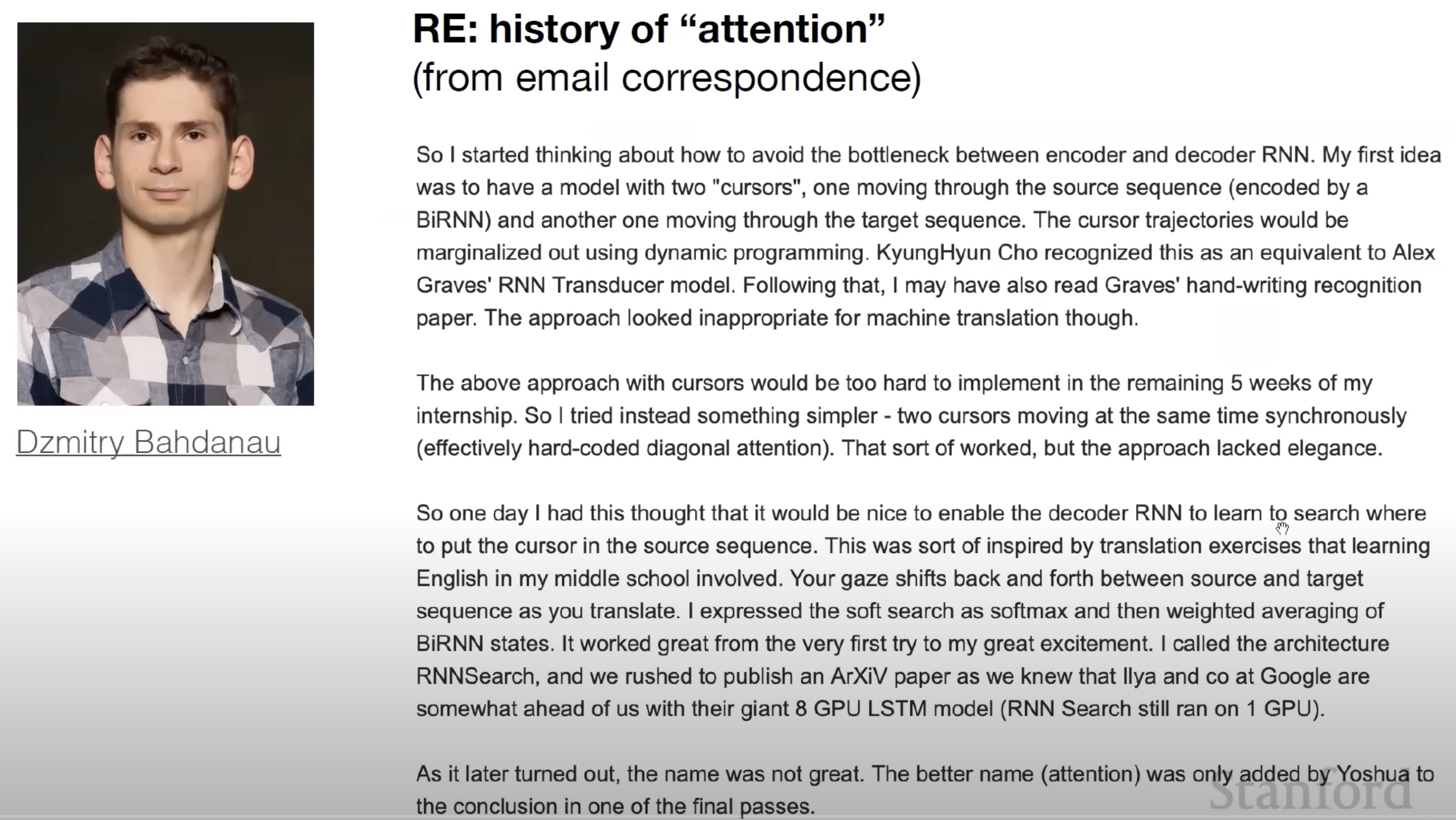
- The following slide from Stanford’s CS25 course shows how the attention mechanism was conceived and is a perfect illustration of why AI/ML is an empirical field, built on intuition.
Attention: Under the hood
- As previously discussed, the role of attention in a model is to strategically focus on pertinent segments of the input sequence as and when required. This ability to tune into relevant sections enhances the model’s overall processing efficiency.
- In a shift from traditional practices, the encoder now funnels a significantly larger amount of data to the decoder. Rather than simply transmitting the last hidden state of the encoding phase, it channels all the hidden states to the decoder, ensuring a more comprehensive data transfer.
- A decoder utilizing attention features undertakes an additional step before generating its output. This step is designed to ensure the decoder’s focus is appropriately honed on parts of the input that are relevant to the current decoding time step. To achieve this, the following operations are performed:
- Each hidden state is multiplied by its respective softmax score. This results in an amplification of hidden states associated with high scores and effectively diminishes the impact of those with low scores. This selective amplification technique supports the model’s ability to maintain focus on the more relevant parts of the input.
- In an encoder, we employ the mechanism of self-attention. This technique allows the model to focus on different parts of the input independently, assisting the overall understanding of the sequence.
- Conversely, in a decoder, cross-attention is applied. This allows the decoder to focus on different parts of the encoder’s output, aiding in the generation of a more accurate translation or summary.
- With each step of the decoding process, a direct connection to the encoder is utilized to strategically zero in on a specific part of the input. This connection enables the model to maintain accuracy while parsing complex sequences.
The Classic Sequence-to-Sequence Model
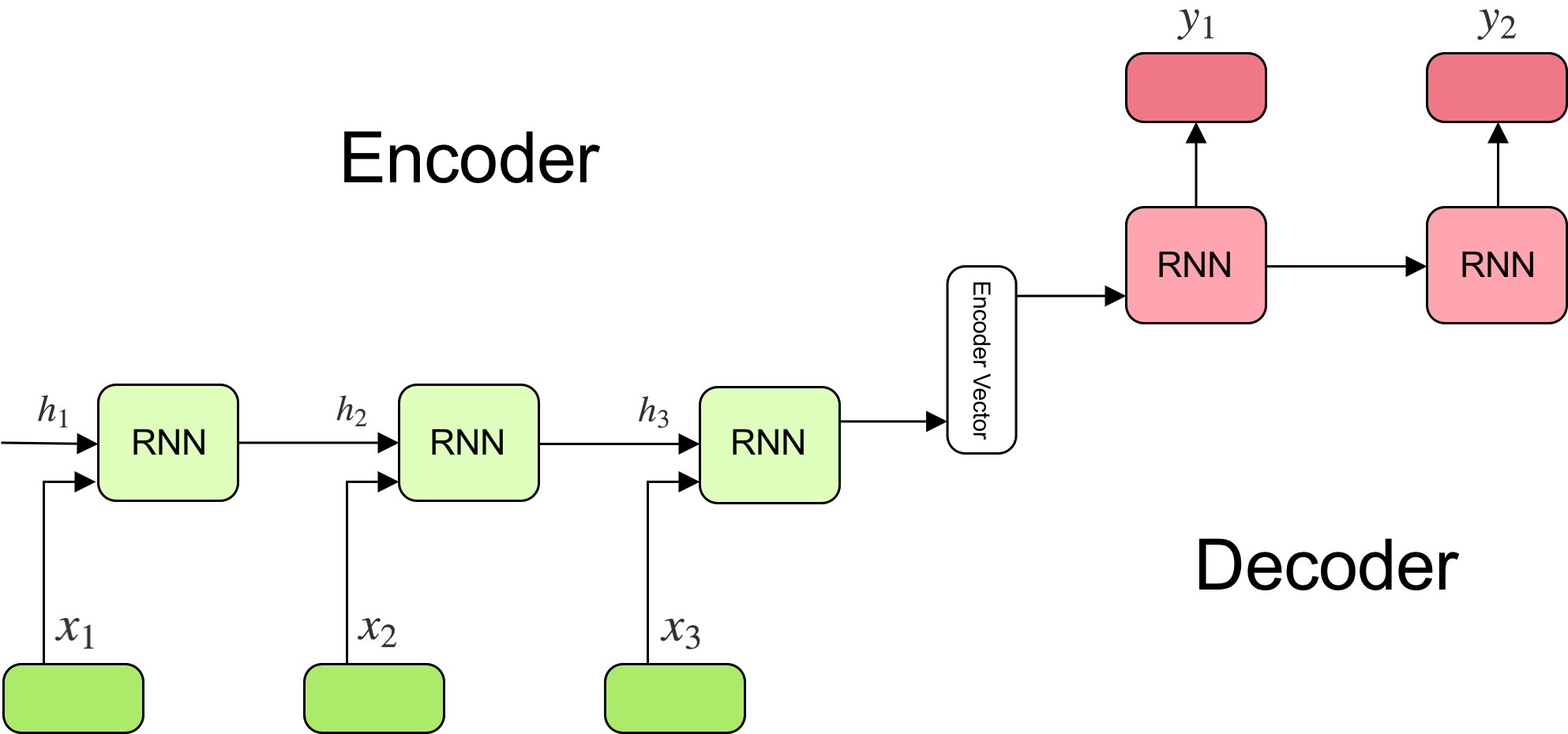
- The seq2seq model is composed of two main components: an encoder, and a decoder, as shown in the figure (source) below:
-
The encoder reads the input sentence, a sequence of vectors \(x = (x_{1}, \dots , x_{T})\), into a fixed-length vector \(c\). The encoder is a recurrent neural network, typical approaches are GRU or LSTMs such that:
\[h_{t} = f\ (x_{t}, h_{t−1})\] \[c = q\ (h_{1}, \dotsc, h_{T})\]- where \(h_{t}\) is a hidden state at time \(t\), and \(c\) is a vector generated from the sequence of the hidden states, and \(f\) and \(q\) are some nonlinear functions.
-
At every time-step \(t\) the encoder produces a hidden state \(h_{t}\), and the generated context vector is modeled according to all hidden states.
-
The decoder is trained to predict the next word \(y_{t}\) given the context vector \(c\) and all the previously predict words \(\{y_{1}, \dots , y_{t-1}\}\), it defines a probability over the translation \({\bf y}\) by decomposing the joint probability:
\[p({\bf y}) = \prod\limits_{i=1}^{x} p(y_{t} | {y_{1}, \dots , y_{t-1}}, c)\]- where \(\bf y = \{y_{1}, \dots , y_{t}\}\). In other words, the probability of a translation sequence is calculated by computing the conditional probability of each word given the previous words. With an LSTM/GRU each conditional probability is computed as:
- where, \(g\) is a nonlinear function that outputs the probability of \(y_{t}\), \(s_{t}\) is the value of the hidden state of the current position, and \(c\) the context vector.
-
In a simple seq2seq model, the last output of the LSTM/GRU is the context vector, encoding context from the entire sequence. This context vector is then used as the initial hidden state of the decoder.
-
At every step of decoding, the decoder is given an input token and (the previous) hidden state. The initial input token is the start-of-string
<SOS>token, and the first hidden state is the context vector (the encoder’s last hidden state). -
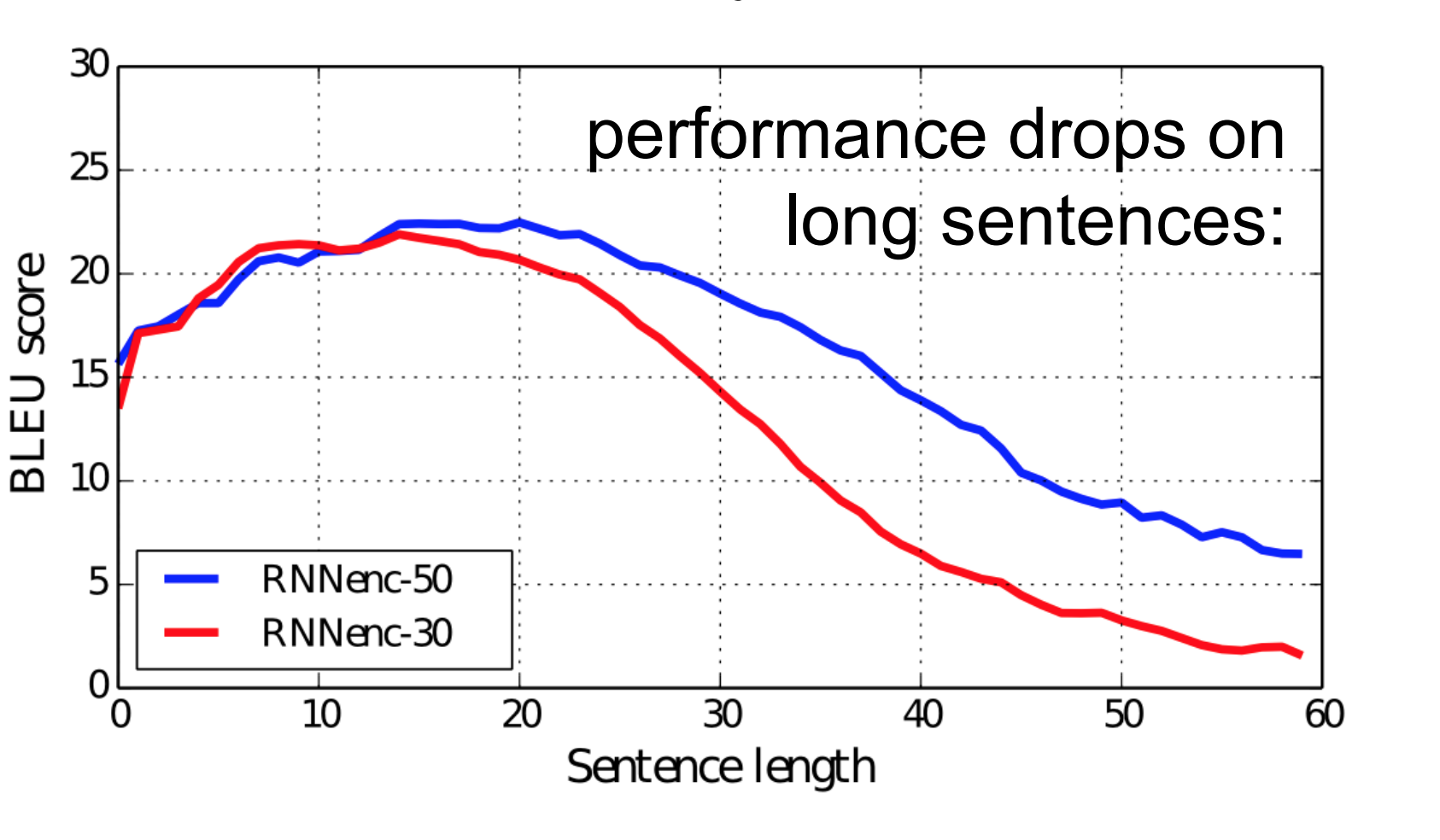
So, the fixed size context-vector needs to contain a good summary of the meaning of the whole source sentence, being this one big bottleneck, specially for long sentences. The figure below (taken from Bahdanau et al. (2015)) shows how the performance of the seq2seq model varies by sentence length:
Sequence-to-Sequence Model with Attention
- The fixed size context-vector bottleneck was one of the main motivations by Bahdanau et al. (2015), which proposed a similar architecture but with a crucial improvement:
“The new architecture consists of a bidirectional RNN as an encoder and a decoder that emulates searching through a source sentence during decoding a translation”
-
The encoder is now a bidirectional recurrent network with a forward and backward hidden states. A simple concatenation of the two hidden states represents the encoder state at any given position in the sentence. The motivation is to include both the preceding and following words in the representation/annotation of an input word.
-
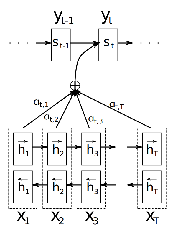
The other key element, and the most important one, is that the decoder is now equipped with some sort of search, allowing it to look at the whole source sentence when it needs to produce an output word, the attention mechanism. The figure below (taken from Bahdanau et al. (2015)) illustrates the attention mechanism in a seq2seq model.
-
The figure above gives a good overview of this new mechanism. To produce the output word at time \(y_{t}\) the decoder uses the last hidden state from the decoder - one can think about this as some sort of representation of the already produced words - and a dynamically computed context vector based on the input sequence.
-
The authors proposed to replace the fixed-length context vector by a another context vector \(c_{i}\) which is a sum of the hidden states of the input sequence, weighted by alignment scores.
-
Note that now the probability of each output word is conditioned on a distinct context vector \(c_{i}\) for each target word \(y\).
-
The new decoder is then defined as:
\[p(y_{t} | {y_{1}, \dots , y_{t-1}}, c) = g(y_{t−1}, s_{i}, c)\]- where \(s_{i}\) is the hidden state for time \(i\), computed by:
- that is, a new hidden state for \(i\) depends on the previous hidden state, the representation of the word generated by the previous state and the context vector for position \(i\). The lingering question now is, how to compute the context vector \(c_{i}\)?
Context Vector
- In attention, the query refers to the word we’re computing attention for. In the case of an encoder, the query vector points to the current input word (aka context).
-
The context vector \(c_{i}\) is a sum of the hidden states of the input sequence, weighted by alignment scores. Each word in the input sequence is represented by a concatenation of the two (i.e., forward and backward) RNNs hidden states, typically referred to as “annotations”.
-
Each annotation contains information about the whole input sequence with a strong focus on the parts surrounding the \(i_{th}\) word in the input sequence.
- The context vector \(c_{i}\) is computed as a weighted sum of these annotations:
-
The weight \(\alpha_{ij}\) of each annotation \(h_{j}\) is computed by:
\[\alpha_{ij} = \text{softmax}(e_{ij})\]- where \(e_{ij} = a(s_{i-1,h_{j}})\)
-
\(a\) is an alignment model which scores how well the inputs around position \(j\) and the output at position \(i\) match. The score is based on the RNN hidden state \(s_{i−1}\) (just before emitting \(y_{i}\) and the \(j_{th}\) annotation \(h_{j}\) of the input sentence
\[a(s_{i-1},h_{j}) = \mathbf{v}_a^\top \tanh(\mathbf{W}_{a}\ s_{i-1} + \mathbf{U}_{a}\ {h}_j)\]- where both \(\mathbf{v}_a\) and \(\mathbf{W}_a\) are weight matrices to be learned in the alignment model.
-
The alignment model in the paper is described as feed forward neural network whose weight matrices \(\mathbf{v}_a\) and \(\mathbf{W}_a\) are learned jointly together with the whole graph/network.
-
The authors note:
“The probability \(\alpha_{ij}h_{j}\) reflects the importance of the annotation \(h_{j}\) with respect to the previous hidden state \(s_{i−1}\) in deciding the next state \(s_{i}\) and generating \(y_{i}\). Intuitively, this implements a mechanism of attention in the decoder.”
Attention vs. fixed-length context vector
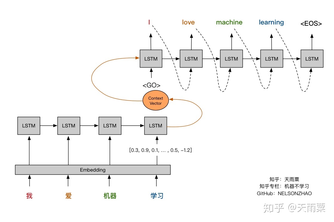
- Let’s visually review the attention mechanism and compare it against the fixed-length context vector approach. The pictures below (credit: Nelson Zhao) help understand the difference between the two encoder-decoder approaches. The figure below illustrates the encoder-decoder architecture with a fixed-context vector.
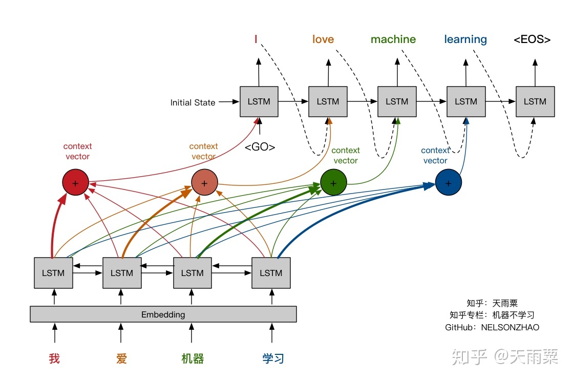
- On the other hand, the figure below illustrates the Encoder-Decoder architecture with attention mechanism proposed in “Neural Machine Translation by Jointly Learning to Align and Translate” by Bahdanau et al. (2015).
Extensions to the Classic Attention Mechanism
- Luong et al. (2015) proposed and compared other mechanisms of attentions, more specifically, alternative functions to compute the alignment score:
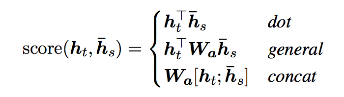
- Note that the concat operation is the same as in Bahdanau et al. (2015); however, instead of a weighted average over all the source hidden states, they proposed a mechanism of local attention which focus only on a small subset of the source positions per target word instead of attending to all words on the source for each target word.
Self-Attention / Scaled Dot-Product Attention
- Earlier, we looked into the “classic” attention mechanism on which subsequent techniques such as self-attention or query-key-value-attention are based.
- After transforming the field of neural machine translation, the attention mechanism was applied to other natural language processing tasks, such as document-level classification or sequence labelling and further extended to other modalities such as vision and speech.
- Please refer the Self-Attention section in our Transformer primer.
Why do we need multiple attention layers?
- Per Eugene Yan’s Some Intuition on Attention and the Transformer blog, multiple attention layers builds in redundancy (on top of having multiple attention heads). If we only had a single attention layer, that attention layer would have to do a flawless job—this design could be brittle and lead to suboptimal outcomes. We can address this via multiple attention layers, where each one uses the output of the previous layer with the safety net of skip connections. Thus, if any single attention layer messed up, the skip connections and downstream layers can mitigate the issue.
- Stacking attention layers also broadens the model’s receptive field. The first attention layer produces context vectors by attending to interactions between pairs of words in the input sentence. Then, the second layer produces context vectors based on pairs of pairs, and so on. With more attention layers, the Transformer gains a wider perspective and can attend to multiple interaction levels within the input sentence.
Comparative Analysis: Additive vs. Scaled Dot-Product Attention
- Among the various types of attention mechanisms, additive attention and scaled dot-product attention are the most commonly used. Here’s a comparison:
Origins and Definitions
- Additive Attention:
- Proposed by Bahdanau et al. in their 2015 paper titled “Neural Machine Translation by Jointly Learning to Align and Translate.”
- It computes the alignment score between the query \(\mathbf{q}\) and the key \(\mathbf{k}\) using a feed-forward neural network with a single hidden layer.
- The formula for the alignment score \(e_{ij}\) is: \(e_{ij} = \mathbf{v}^{T} \tanh(\mathbf{W}_{q}\mathbf{q}_i + \mathbf{W}_{k}\mathbf{k}_j)\)
- Here, \(\mathbf{W}_{q}\) and \(\mathbf{W}_{k}\) are learnable weight matrices, and \(\mathbf{v}\) is a learnable vector.
- Scaled Dot-Product Attention:
- Introduced in Attention Is All You Need by Vaswani et al. in 2017.
- It computes the alignment score by taking the dot product of the query and key vectors, scaled by the square root of the dimension of the key vectors (\(d_k\)).
- The formula for the alignment score \(e_{ij}\) is: \(e_{ij} = \frac{\mathbf{q}_i \cdot \mathbf{k}_j}{\sqrt{d_{k}}}\)
Computational Efficiency
- Additive Attention:
- Involves a more complex computation due to the use of a feed-forward network.
- While theoretically similar in complexity to dot-product attention, it is generally slower in practice because it cannot leverage highly optimized matrix multiplication libraries.
- Requires additional parameters \(\mathbf{W}_{q}\), \(\mathbf{W}_{k}\), and \(\mathbf{v}\), increasing memory usage.
- Scaled Dot-Product Attention:
- Much faster and more space-efficient as it relies on matrix multiplication, which is highly optimized in modern deep learning libraries (e.g., TensorFlow, PyTorch).
- The scaling factor \(\frac{1}{\sqrt{d_{k}}}\) helps to mitigate the issue of having large dot product values, which can lead to small gradients during backpropagation.
Theoretical Complexity
- Both attention mechanisms have a theoretical time complexity of \(O(n^2 \cdot d)\), where \(n\) is the sequence length and \(d\) is the dimension of the representations.
- However, in practice:
- Additive Attention involves additional computation for the feed-forward network, which can slow down the process.
- Scaled Dot-Product Attention benefits from efficient matrix multiplication operations, making it faster in real-world applications.
Usage and Performance
- Additive Attention:
- Often used in earlier models of neural machine translation and other NLP tasks before the advent of the Transformer architecture.
- Still useful in scenarios where the performance benefits of dot-product attention do not outweigh its simplicity and interpretability.
- Scaled Dot-Product Attention:
- Integral to the Transformer architecture, which has become the standard for many NLP tasks.
- Scales better with larger datasets and more complex models, leading to state-of-the-art performance in a wide range of applications.
Implementation Details
- Additive Attention:
- Typically implemented with separate weight matrices for the query and key vectors, followed by a non-linear activation (e.g., \(\tanh\)) and a final linear layer to compute the score.
- Example pseudocode:
def additive_attention(query, key):
    w_q = nn.Linear(query_dim, hidden_dim)
    w_k = nn.Linear(key_dim, hidden_dim)
    v = nn.Linear(hidden_dim, 1)
    scores = v(tanh(w_q(query) + w_k(key)))
    attention_weights = softmax(scores, dim=-1)
    return attention_weights
- Scaled Dot-Product Attention:
- Implemented using matrix multiplication followed by a scaling factor and softmax function to compute the attention weights.
- Example pseudocode:
def scaled_dot_product_attention(query, key, value, mask=None):
    d_k = query.size(-1)
    scores = torch.matmul(query, key.transpose(-2, -1)) / math.sqrt(d_k)
    if mask is not None:
        scores = scores.masked_fill(mask == 0, -1e9)
    attention_weights = softmax(scores, dim=-1)
    output = torch.matmul(attention_weights, value)
    return output
Conclusion
- Additive Attention is more complex and computationally intensive but has been foundational in early NLP models.
- Scaled Dot-Product Attention is faster, more efficient, and scalable, making it the preferred choice in modern architectures like Transformers.
- The choice between the two often depends on the specific application requirements and the computational resources available. However, for most state-of-the-art NLP tasks, scaled dot-product attention is the go-to mechanism due to its performance and efficiency advantages.
Multi-Head Attention
- Please refer the Multi-Head Attention section in our Transformer primer.
Cross Attention
- Please refer the Cross Attention section in our Transformer primer.
Ghost Attention
- The authors of Llama 2 proposed Ghost Attention (GAtt).
- Ghost Attention (GAtt) is an innovative technique specifically designed to aid LLMs in remembering and adhering to initial instructions throughout a conversation. This methodology extends the notion of Context Distillation, where specific details are distilled and highlighted from the broader context to enhance understanding.
- Context Distillation is a concept that focuses on highlighting and isolating specific, crucial details from a larger and more complex context. This process is similar to distilling, where the essential elements are extracted from a compound mixture.Context Distillation is used to introduce and retain an instruction throughout a dialogue. This helps the model to consistently remember and adhere to the instruction, enhancing its ability to maintain focus and perform accurately.
- In this technique, an instruction - a directive that must be consistently followed during the entire dialogue - is added to all user messages in a synthetic dialogue dataset. However, during the training phase, the instruction is only retained in the first turn of the dialogue and the loss (a measure of error) is set to zero for all tokens (representative units of information) from earlier turns.
- The authors applied this unique approach across a variety of synthetic constraints, which included diverse elements like hobbies, languages, and public figures. Implementing GAtt effectively preserved attention on initial instructions for a significantly larger portion of the conversation, ensuring that the AI stayed focused on its tasks.
- One of the notable achievements of GAtt is its ability to maintain consistency in adhering to initial instructions even over extended dialogues, comprising more than 20 turns, until it hits the maximum context length that the model can handle. While this first iteration has proven successful, the authors believe that there is ample room for further refinement and improvement, suggesting that the Ghost Attention technique can continue to evolve for enhanced performance.
- Let’s say we are training a dialogue system to book appointments for a dental clinic, and one of the rules we want the system to follow is that it should always inquire about the patient’s dental insurance details.
- In the synthetic dialogue dataset used for training, we append the instruction “Always ask about dental insurance” to every user message.
- For example:
- User: “I need an appointment.”
- AI (with instruction): “Always ask about dental insurance. Sure, I can help you with that. Do you have a preferred date and time?”
- User: “How about next Tuesday at 10 am?”
- AI (with instruction): “Always ask about dental insurance. That time works. May I also ask if you have dental insurance and, if so, could you provide the details?”
-
During training, GAtt retains this instruction only in the first turn and sets the loss to zero for all tokens from earlier turns. The model will be trained to understand that asking about dental insurance is an important part of the conversation, and it should remember this instruction even in later turns.
- For example, when the model is actually deployed:
- User: “I need an appointment.”
- AI: “Sure, I can help you with that. Do you have a preferred date and time?”
- User: “How about next Tuesday at 10 am?”
- AI: “That time works. May I also ask if you have dental insurance and, if so, could you provide the details?”
- Notice that even though the instruction “Always ask about dental insurance” is not explicitly mentioned during the conversation after training, the AI system consistently adheres to it throughout the dialogue, as it has been trained using GAtt.
- This technique ensures the AI model stays focused on the initial instruction, in this case, asking about dental insurance, enhancing its dialogue capabilities and making it more reliable for the task at hand.
Attention in Today’s Frontier LLMs
- While the Transformers of 2017 implemented attention computation that scaled quadratically, this no longer holds true with recent Transformer models.
- Significant advancements have been made in the computation of attentions since the introduction of GPT-3. Most large language models now employ sub-quadratic attention mechanisms, and many implementations have achieved constant space complexity. Innovations such as Paged-Attention and Flash Attention have allowed for more efficient read-write access on hardware. Consequently, many open-source projects have moved beyond standard PyTorch implementations to accommodate enhanced hardware utilization.
Linear Attention
- Proposed in Linformer: Self-Attention with Linear Complexity by Wang et al. from Facebook AI.
- The authors proposes a novel approach to optimizing the self-attention mechanism in Transformer models, reducing its complexity from quadratic to linear with respect to sequence length. This method, named Linformer, maintains competitive performance with standard Transformer models while significantly enhancing efficiency in both time and memory usage.
- Linformer introduces a low-rank approximation of the self-attention mechanism. By empirically and theoretically demonstrating that the self-attention matrix is of low rank, the authors propose a decomposition of the original scaled dot-product attention into multiple smaller attentions via linear projections. This factorization effectively reduces both the space and time complexity of self-attention from \(O(n^2)\) to \(O(n)\), addressing the scalability issues of traditional Transformers.
- The model architecture involves projecting key and value matrices into lower-dimensional spaces before computing the attention, which retains the model’s effectiveness while reducing computational demands. The approach includes options for parameter sharing across projections, which can further reduce the number of trainable parameters without significantly impacting performance.
-
In summary, here’s how Linformer achieves linear-time attention:
-
Low-Rank Approximation: The core idea behind Linformer is the observation that self-attention can be approximated by a low-rank matrix. This implies that the complex relationships captured by self-attention in Transformers do not necessarily require a full rank matrix, allowing for a more efficient representation.
-
Reduced Complexity: While standard self-attention mechanisms in Transformers have a time and space complexity of \(O(n^2)\) with respect to the sequence length (n), Linformer reduces this complexity to \(O(n)\). This significant reduction is both in terms of time and space, making it much more efficient for processing longer sequences.
-
Mechanism of Linear Self-Attention: The Linformer achieves this by decomposing the scaled dot-product attention into multiple smaller attentions through linear projections. Specifically, it introduces two linear projection matrices \(E_i\) and \(F_i\) which are used when computing the key and value matrices. By first projecting the original high-dimensional key and value matrices into a lower-dimensional space (\(n \times k\)), Linformer effectively reduces the complexity of the attention mechanism.
-
Combination of Operations: The combination of these operations forms a low-rank factorization of the original attention matrix. Essentially, Linformer simplifies the computational process by approximating the full attention mechanism with a series of smaller, more manageable operations that collectively capture the essential characteristics of the original full-rank attention.
-
- The figure below from the paper shows: (left and bottom-right) architecture and example of the proposed multihead linear self-attention; (top right) inference time vs. sequence length the various Linformer models.

- Experimental validation shows that Linformer achieves similar or better performance compared to the original Transformer on standard NLP tasks such as sentiment analysis and question answering, using datasets like GLUE and IMDB reviews. Notably, the model offers considerable improvements in training and inference speeds, especially beneficial for longer sequences.
- Additionally, various strategies for enhancing the efficiency of Linformer are tested, including different levels of parameter sharing and the use of non-uniform projected dimensions tailored to the specific demands of different layers within the model.
- The authors suggest that the reduced computational requirements of Linformer not only make high-performance models more accessible and cost-effective but also open the door to environmentally friendlier AI practices due to decreased energy consumption.
- In summary, Linformer proposes a more efficient self-attention mechanism for Transformers by leveraging the low-rank nature of self-attention matrices. This approach significantly reduces the computational burden, especially for long sequences, by lowering the complexity of attention calculations from quadratic to linear in terms of both time and space. This makes Linformer an attractive choice for tasks involving large datasets or long sequence inputs, where traditional Transformers might be less feasible due to their higher computational demands.
Lightning Attention
Algorithm
- The lightning attention mechanism is a highly optimized implementation of linear attention, designed to achieve both linear complexity and scalability across long sequence lengths. Below is the detailed algorithm used for the forward pass of lightning attention.
Core Steps
- Input Partitioning:
- The input matrices \(Q\), \(K\), and \(V\) are divided into blocks of size \(B \times d\), where \(B\) is the block size, and \(d\) is the feature dimension.
- Initialization:
- Initialize a cumulative key-value matrix \(KV = 0\) of shape \(d \times d\).
- Create a mask \(M\) to handle causal attention, where \(M_{ts} = 1\) if \(t \geq s\), otherwise 0.
- Block-Wise Computation:
- For each block \(t\):
- Intra-Block Attention: Compute intra-block attention scores using the left product operation.
- Inter-Block Attention: Update the cumulative key-value matrix \(KV\) and compute the inter-block contributions using the right product operation.
- Combine the intra- and inter-block results to produce the final output for the block.
- For each block \(t\):
- Output Assembly:
- Concatenate the outputs of all blocks to form the final output matrix \(O\).
Lightning Attention Forward Pass
- The following figure from the paper shows the algorithm for the lightning attention forward pass:
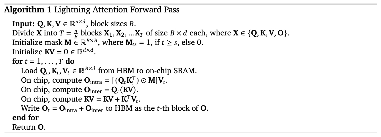
- Input: Query (\(Q\)), Key (\(K\)), Value (\(V\)) matrices of shape \((n, d)\), block size (\(B\))
-
Output: Output matrix (\(O\)) of shape \((n, d)\)
-
Steps:
- Initialize:
- Cumulative Key-Value matrix (\(KV = 0\)) of shape \((d, d)\)
- Causal mask \(M\) for intra-block operations
- Output matrix \(O\) of shape \((n, d)\)
-
Divide \(Q\), \(K\), and \(V\) into \(T = \lceil n / B \rceil\) blocks.
- For each block \(t \in [1, T]\):
- Extract current block \(Q_t, K_t, V_t\).
- Compute Intra-Block Attention using: \(O_{\text{intra}} = (Q_t K_t^T \odot M)V_t\)
- Compute Inter-Block Attention using: \(O_{\text{inter}} = Q_t KV\)
- Update \(KV\) with: \(KV = KV + K_t^T V_t\)
- Combine results: \(O_t = O_{\text{intra}} + O_{\text{inter}}\)
- Return \(O\).
- Initialize:
Pseudocode for Lightning Attention
def lightning_attention(Q, K, V, block_size):
    """
    Lightning Attention Forward Pass
    Args:
        Q: Query matrix of shape (n, d)
        K: Key matrix of shape (n, d)
        V: Value matrix of shape (n, d)
        block_size: Size of each block (B)
    Returns:
        O: Output matrix of shape (n, d)
    """
    n, d = Q.shape  # Sequence length and feature dimension
    num_blocks = (n + block_size - 1) // block_size  # Total number of blocks
    KV = np.zeros((d, d))  # Initialize cumulative key-value matrix
    mask = np.tril(np.ones((block_size, block_size)))  # Causal mask

    # Initialize the output matrix
    O = np.zeros_like(Q)

    for t in range(num_blocks):
        # Load current block
        start = t * block_size
        end = min((t + 1) * block_size, n)
        Q_t = Q[start:end, :]
        K_t = K[start:end, :]
        V_t = V[start:end, :]

        # Intra-block computation (left product)
        intra_block = (Q_t @ K_t.T * mask[:end - start, :end - start]) @ V_t

        # Inter-block computation (right product)
        inter_block = Q_t @ KV

        # Update cumulative key-value matrix
        KV += K_t.T @ V_t

        # Combine intra- and inter-block results
        O[start:end, :] = intra_block + inter_block

    return O
Multi-Query Attention
-
Introduced in Fast Transformer Decoding: One Write-Head is All You Need by Shazeer et al. (2019), Multi-Query Attention (MQA) is an architectural modification to the standard multi-head attention mechanism that improves efficiency — particularly for inference in large-scale language models.
-
In standard multi-head attention, each head maintains its own set of query, key, and value projections. While powerful, this design has a significant memory and compute cost, especially at inference time due to the need to cache separate keys and values for each head. MQA addresses this by sharing the keys and values across all heads, while keeping the queries distinct per head. This drastically reduces the memory footprint during decoding because only one set of key and value vectors needs to be stored per time step across all heads, rather than one per head.
Why Multi-Query Attention Works
- Queries are still head-specific, allowing the model to attend to different aspects of the input.
- Since keys and values are typically derived from the same source sequence, they often exhibit redundancy across heads. MQA leverages this by reusing them, saving space without a major performance trade-off.
- Empirical results show that MQA retains model quality while reducing memory bandwidth and improving cache locality — both important for fast autoregressive generation.
Benefits of Multi-Query Attention
- Reduced KV Cache Size: Particularly important during inference in LLMs, where caching key-value pairs for long contexts can consume vast amounts of memory.
- Faster Decoding: Fewer operations and better hardware utilization lead to faster inference times.
- Scalability: Enables training and deploying larger models without linearly increasing inference costs.
Use in Modern Models
- MQA has been widely adopted in production models and open-source LLMs such as PaLM, Llama, and Mistral. Some models also employ Grouped-Query Attention (GQA) — a compromise between full multi-head attention and MQA, where queries are grouped and share keys/values within each group.
- In summary, Multi-Query Attention offers a highly efficient alternative to traditional attention in decoder-only architectures, enabling faster inference with minimal accuracy trade-offs — a key innovation for scaling large language models in practical settings.
Sliding Window Multi-Query Attention
- Introduced in Mistral 7B, Sliding Window Multi-Query Attention (SW-MQA) combines the memory efficiency of MQA with the locality-aware design of Sliding Window Attention. This mechanism is purpose-built for fast and scalable inference in long-context Transformer models, such as Mistral-7B, where attention is restricted to a fixed window of preceding tokens while keys and values are shared across all heads.
Motivation and Design
-
Traditional full self-attention with causal masking allows every token to attend to all previous tokens, which results in quadratic time and memory complexity. While this ensures full context availability, it becomes computationally prohibitive for long sequences.
-
Sliding Window Attention addresses this by restricting each token to attend only to the \(W\) most recent tokens, where \(W\) is the window size. This keeps attention causal and local, with time complexity reduced to \(O(NW)\). To recover long-range information, multiple stacked layers are used: information propagates up to \(W\) tokens per layer, meaning a Transformer with L layers can propagate information across up to \(L \times W\) tokens.
-
Additionally, Multi-Query Attention (MQA) reduces the number of key/value projections to one set per layer (shared across all heads), dramatically lowering KV cache size and improving inference speed. Combining MQA with sliding window locality further enhances both hardware efficiency and scalability.
Example: Progressive Information Flow
-
Consider a Transformer with:
- 10-token input
- 4 layers
- Window size W = 4
-
Then:
- Layer 1: Token T4 can attend to T1–T4
- Layer 2: Token T6 can indirectly access T2–T6
- Layer 3: Token T9 now accesses T5–T9 (which includes indirect info from earlier tokens)
- Layer 4: Full context propagation from T0 to T9 is complete
-
Thus, even with limited local attention per layer, stacking enables global information flow by the final layer.
Implementation Overview
- Below is a simplified breakdown of how Sliding Window Multi-Query Attention is implemented in Mistral:
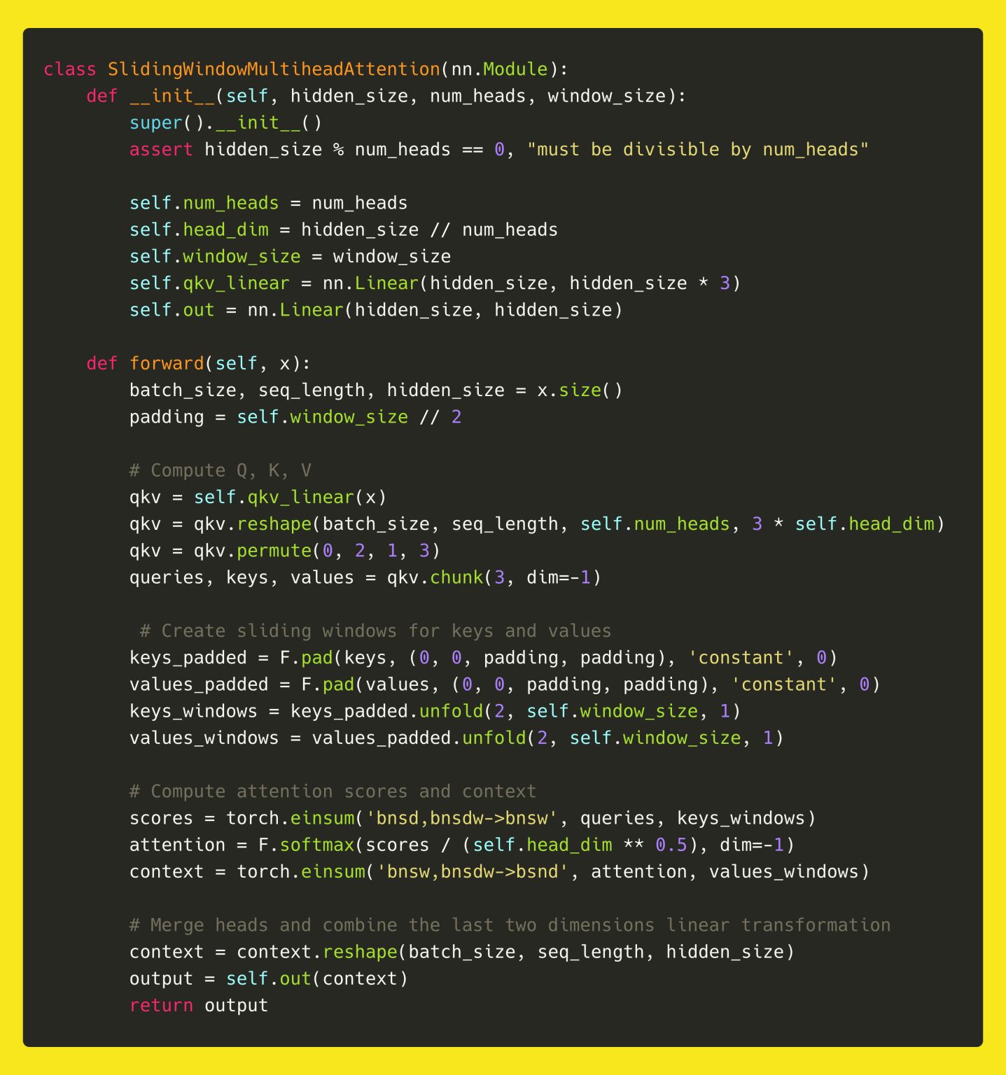
-
Initialization:
- The attention module is initialized with parameters like
hidden_size,num_heads, andwindow_size. - A single linear layer projects inputs into queries, keys, and values (
qkv_linear). - An output projection layer (
out) transforms the final attention output.
- The attention module is initialized with parameters like
-
Forward Pass:
- Reshape Inputs: Batch inputs into query, key, and value tensors.
- Sliding Window Padding: Keys and values are padded to allow windowed lookups at the sequence boundaries.
- Window Unfolding: Keys and values are “unfolded” into overlapping chunks of size \(W\), aligned with the sliding window.
- Attention Scores: Queries are dotted with windowed keys, scaled, and passed through softmax.
- Weighted Sum: The resulting weights are used to compute a windowed attention-weighted sum over values.
- Merge Heads: Attention outputs from all heads are concatenated and projected back to the hidden size.
-
Memory and Efficiency:
- Because keys and values are shared across all heads (as in MQA), only one KV set is cached per sequence position — reducing both compute and memory usage.
- In summary, Sliding Window Multi-Query Attention strikes a pragmatic balance between contextual richness and runtime efficiency. It enables modern LLMs to operate over long sequences at scale, preserving causality, exploiting locality, and minimizing memory overhead — all while maintaining competitive performance.
Grouped-Query Attention
-
Introduced in GQA: Training Generalized Multi-Query Transformer Models from Multi-Head Checkpoints by Ainslie et al. (2023), Grouped-Query Attention (GQA) is a middle ground between full multi-head attention and multi-query attention, designed to balance efficiency and model expressiveness.
-
In GQA, the queries are divided into groups, where each group shares the same key and value projections. Unlike Multi-Query Attention (MQA), which uses one shared key/value pair for all heads, GQA introduces \(G\) shared key-value sets, where \(G < H\), and \(H\) is the number of heads.
-
The following figure from the paper presents an overview of grouped-query method. Multi-head attention has \(H\) query, key, and value heads. Multi-query attention shares single key and value heads across all query heads. Grouped-query attention instead shares single key and value heads for each group of query heads, interpolating between multi-head and multi-query attention.
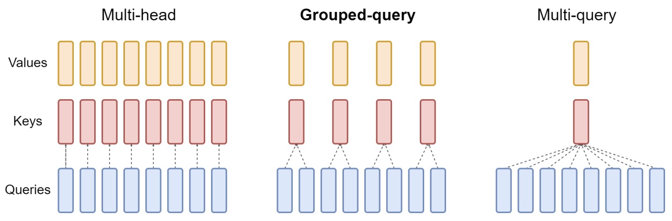
- This approach retains some diversity in key-value representation while significantly reducing the memory and compute overhead compared to full multi-head attention.
Motivation and Benefits
- Better Trade-off: GQA offers a spectrum between the full expressiveness of multi-head attention and the efficiency of MQA.
- Memory Efficiency: Reduces the number of key-value projections to \(G\) instead of \(H\), lowering the memory and caching requirements during autoregressive decoding.
- Improved Parallelism: As shown in the FlashAttention-2 implementation, this structure allows better batching and tiling for GPU operations, leading to faster inference and training.
How it Works
-
Suppose a Transformer model has:
- \(H = 16\) attention heads
- \(G = 4\) query groups
-
Each group of 4 heads shares the same key and value projections. So:
- 16 different query projections (1 per head)
- 4 key projections and 4 value projections (1 per group)
-
This means the memory and compute for keys and values is reduced by a factor of 4, while retaining more flexibility than MQA.
Adoption in Modern LLMs
-
GQA is now widely adopted in large language models like Llama 2/3/4, Mistral, and Gemma, where models use a high number of attention heads but a smaller number of key-value groups to strike a balance between hardware efficiency and attention diversity.
-
In essence, Grouped-Query Attention provides a scalable, efficient design for large Transformer models, enabling high-throughput inference without a large sacrifice in performance — making it a compelling choice in modern LLM engineering.
Multi-Head vs. Multi-Query vs. Grouped-Query Attention
-
With the growing scale of language models and demand for fast inference, attention mechanisms have evolved to balance expressiveness, efficiency, and memory usage. Three primary variants dominate this design space:
- MHA: Each attention head has its own set of query, key, and value projections.
- MQA: All heads share a single set of key and value projections, while queries remain distinct.
- GQA: Heads are divided into groups; each group shares keys and values, but not queries.
-
These designs are widely used across modern Transformer models, depending on architectural goals and deployment constraints.
Key Differences
- MHA provides the highest flexibility and modeling capacity but with the most memory and compute cost.
- MQA is the most efficient in terms of memory and decoding speed but sacrifices some diversity across attention heads.
- GQA offers a balanced trade-off by reducing key-value redundancy while maintaining some head-level diversity.
Comparative Analysis
- The table below compares MHA, MQA, and GQA in terms of structure, performance, and resource efficiency. Let \(H\) denote the number of attention heads, and \(G\) the number of query groups, with \(G < H\).
| Feature | Multi-Head Attention (MHA) | Multi-Query Attention (MQA) | Grouped-Query Attention (GQA) |
|---|---|---|---|
| Query Projections | One per head (\(H\) total) |
One per head (\(H\) total) |
One per head (\(H\) total) |
| Key/Value Projections | One per head (\(H\) total) |
Shared across all heads (1 KV pair) |
Shared per group (\(G\) KV pairs) |
| Memory Usage (KV Cache) | High (cache stores \(H\) KV sets) |
Low (cache stores 1 KV set) |
Medium (cache stores \(G\) KV sets) |
| Inference Speed | Slowest | Fastest | Faster than MHA, slower than MQA |
| Model Expressiveness | Highest | Lowest | Middle ground |
| Hardware Efficiency | Least efficient | Most efficient | Efficient |
| Used In | GPT-2, BERT, T5 | PaLM, Llama, Mistral | Llama 2, Gemma, Mistral |
- In summary, MHA remains the gold standard for rich contextual modeling, while MQA and GQA are engineering innovations driven by the needs of scaling, efficiency, and hardware constraints — crucial for the deployment of modern LLMs in real-world environments.
Complexity Analysis
- Both MQA and GQA reduce the quadratic scaling bottlenecks of standard multi-head attention and are considered sub-quadratic in inference-time memory and compute, under typical decoder-only (autoregressive) settings, especially advantageous in long-context autoregressive inference scenarios. However, each one of them comes with its own set of caveats.
MQA
- Key design: Only one set of keys and values is computed and cached, regardless of the number of attention heads.
-
Memory and compute savings:
- Memory: KV cache is reduced from \(O(H × L × d)\) to \(O(L × d)\) (where \(H\) = number of heads, \(L\) = sequence length, \(d\) = head dimension).
- Compute: During decoding, the attention lookup is linear in sequence length \(O(L)\) per token.
- Result: MQA makes inference sub-quadratic — in fact, linear with respect to sequence length for each token step.
GQA
- Key design: KV projections are shared within groups of attention heads. So, with \(G\) groups, you store only \(G\) sets of keys/values, where \(G < H\).
-
Memory and compute:
- Memory: KV cache size is \(O(G × L × d)\) — better than MHA, but larger than MQA.
- Compute: Like MQA, per-token attention cost during decoding is \(O(L)\) per head, with reduced KV lookup.
- Result: GQA is also sub-quadratic, with a tunable balance between memory efficiency (via \(G\)) and expressiveness.
Tabular Summary
| Attention Type | KV Cache Size | Inference Time Complexity | Sub-Quadratic? |
|---|---|---|---|
| MHA | \(O(H \times L \times d)\) | \(O(H \times L)\) per token | ❌ (Quadratic) |
| MQA | \(O(L \times d)\) | \(O(L)\) per token | ✅ (Linear) |
| GQA | \(O(G \times L \times d)\) | \(O(G \times L)\) per token | ✅ (Sub-Quadratic) |
Multi-Head Latent Attention (MLA)
- The Multi-Head Latent Attention (MLA) mechanism was proposed in DeepSeek-V3 is a refined adaptation of the traditional multi-head attention. MLA focuses on compressing the key-value (KV) cache and reducing activation memory, enabling efficient inference without significant performance degradation.
Key Equations and Design
-
Let \(d\) denote the embedding dimension, \(n_h\) the number of attention heads, and \(d_h\) the dimension per head. Given the attention input for the \(t^{th}\) token at a specific attention layer, \(h_t \in \mathbb{R}^d\), MLA introduces a low-rank joint compression mechanism for both keys and values. The primary components are:
- Compressed Latent Vector for Keys and Values:
\(c_{KV_t} = W_{DKV} h_t\)
- where \(c_{KV_t} \in \mathbb{R}^{d_c}\) is the compressed latent vector, \(d_c \ll d_h n_h\), and \(W_{DKV} \in \mathbb{R}^{d_c \times d}\) is the down-projection matrix.
- Key Representations:
\(k_C = W_{UK} c_{KV_t}, \quad k_R = \text{RoPE}(W_{KR} h_t), \quad k_t = [k_C; k_R]\)
- where \(W_{UK}\) and \(W_{KR}\) are up-projection matrices, and \(\text{RoPE}(\cdot)\) applies Rotary Positional Embeddings (RoPE). \(k_t\) concatenates compressed \(k_C\) and \(k_R\).
-
Value Representations: \(v_C = W_{UV} c_{KV_t}\)
- Query Compression:
Similarly, queries are compressed using:
\(c_{Q_t} = W_{DQ} h_t, \quad q_C = W_{UQ} c_{Q_t}, \quad q_R = \text{RoPE}(W_{QR} c_{Q_t}), \quad q_t = [q_C; q_R]\)
- where \(W_{DQ}\), \(W_{UQ}\), and \(W_{QR}\) are respective projection matrices for queries.
- Final Attention Output:
The output \(u_t\) for the \(t^{th}\) token is computed as:
\(o_{t,i} = \sum_{j=1}^{t} \text{Softmax}_j \left( \frac{q_{t,i}^\top k_{j,i}}{\sqrt{d_h + d_R}} \right) v_{C,j,i}, \quad u_t = W_O [o_{t,1}; o_{t,2}; \dots; o_{t,n_h}]\)
- where \(W_O \in \mathbb{R}^{d \times d_h n_h}\) is the output projection matrix.
- Compressed Latent Vector for Keys and Values:
\(c_{KV_t} = W_{DKV} h_t\)
Implementation Details
-
KV Cache Reduction: Only the compressed latent vectors \(c_{KV_t}\) and \(k_R\) need to be cached during inference. This significantly reduces the KV cache size, especially for models with large sequences or extensive parameterization.
-
Query Compression: Similar to KV compression, query representations are also compressed, reducing activation memory during training.
- Performance Optimization:
Despite the reduced cache and memory requirements, MLA achieves performance comparable to traditional multi-head attention through:
- Efficient RoPE application for positional encoding.
- Proper scaling and projection mechanisms to preserve information fidelity.
- Inference Efficiency: By caching only the compressed representations, MLA minimizes memory overhead during inference while maintaining the ability to focus dynamically on the most relevant tokens.
References
- An Introductory Survey on Attention Mechanisms in NLP Problems (arXiv.org version)
- Neural Machine Translation by Jointly Learning to Align and Translate (slides)
- Effective Approaches to Attention-based Neural Machine Translation (slides)
- “Attention, Attention” in Lil’Log
- Big Bird: Transformers for Longer Sequences
- Paper Review: Llama 2: Open Foundation and Fine-Tuned Chat Models
- “Attention” in Eugene Yan
Citation
If you found our work useful, please cite it as:
@article{Chadha2021DistilledAttention,
  title   = {Attention},
  author  = {Jain, Vinija and Chadha, Aman},
  journal = {Aman's AI Journal},
  year    = {2021},
  note    = {\url{https://aman.ai}}
}