Primers • Transformers
- Background: Representation Learning for Natural Language Processing
- Enter the Transformer
- Transformers vs. Recurrent and Convolutional Architectures: An Overview
- Breaking Down the Transformer
- Background
- One-Hot Encoding
- Dot product
- Matrix Multiplication as a Series of Dot Products
- First-Order Sequence Model
- Second-Order Sequence Model
- Second-Order Sequence Model with Skips
- Masking Features
- From Feature Vectors to Transformers
- Attention as Matrix Multiplication
- Second-Order Sequence Model as Matrix Multiplications
- Sampling a Sequence of Output Words
- Transformer Core
- Embeddings
- Positional Encoding
- Decoding Output Words / De-Embeddings / Un-Embeddings
- Attention
- Dimensional Restrictions on Queries, Keys, and Values
- Why attention? Contextualized Word Embeddings
- Types of Attention: Additive, Multiplicative (Dot-product), and Scaled
- Attention calculation
- Self-Attention
- Single Head Attention Revisited
- Why is the product of the \(Q\) and \(K\) matrix in Self-Attention normalized?
- Coding up self-attention
- Averaging is equivalent to uniform attention
- Activation Functions
- Attention in Transformers: What is new and what is not?
- Calculating \(Q\), \(K\), and \(V\) matrices in the Transformer architecture
- Calculating \(Q\), \(K\), and \(V\) matrices in the Transformer architecture
- Optimizing Performance with the KV Cache
- Applications of Attention in Transformers
- Multi-Head Attention
- Cross-Attention
- Dropout
- Skip connections
- Layer Normalization
- Comparison of Normalization Techniques
- Pre-Norm vs. Post-Norm Transformer Architectures
- Why Transformer Architectures Use Layer Normalization
- How Layer Normalization Works Compared to Batch Normalization
- Why Transformers Use Layer Normalization vs. Other Forms
- Related: Modern Normalization Alternatives for Transformers (such as RMSNorm, ScaleNorm, and AdaNorm)
- Softmax
- Stacking Transformer Layers
- Transformer Encoder and Decoder
- Putting it all together: The Transformer Architecture
- Loss Function
- Background
- Implementation details
- Tokenization
- Byte Pair Encoding (BPE)
- Teacher Forcing
- Shift Right (Off-by-One Label Shift) in Decoder Inputs
- Scheduled Sampling
- Label Smoothing as a Regularizer
- Scaling Issues
- Adding a New Token to the Tokenizer’s Vocabulary and Model’s Embedding Table
- Extending the Tokenizer to New Languages
- End-to-end flow: from input embeddings to next-token prediction
- Step 1: Tokenization \(\rightarrow\) token IDs
- Step 2: Token embeddings and positional encoding
- Step 3: Stack of \(L\) Transformer decoder layers
- Step 4: Select the final token representation
- Step 5: Projection to vocabulary logits
- Step 6: Softmax and token selection
- Step 7: Autoregressive generation loop
- Step 8: Key–value (KV) caching for efficient inference
- The relation between transformers and Graph Neural Networks
- Time complexity: RNNs vs. Transformers
- Lessons Learned
- Transformers: merging the worlds of linguistic theory and statistical NLP using fully connected graphs
- Long term dependencies
- Are Transformers learning neural syntax?
- Why multiple heads of attention? Why attention?
- Benefits of Transformers compared to RNNs/GRUs/LSTMs
- What would we like to fix about the transformer? / Drawbacks of Transformers
- Why is training Transformers so hard?
- Transformers: Extrapolation engines in high-dimensional space
- The road ahead for Transformers
- Choosing the right language model for your NLP use-case: key takeaways
- Transformers Learning Recipe
- Transformers From Scratch
- The Illustrated Transformer
- Lilian Weng’s The Transformer Family
- The Annotated Transformer
- Attention Is All You Need
- HuggingFace Encoder-Decoder Models
- Transformers library by HuggingFace
- Inference Arithmetic
- Transformer Taxonomy
- GPT in 60 Lines of NumPy
- x-transformers
- Speeding up the GPT - KV cache
- Transformer Poster
- FAQs
- In Transformers, how does categorical cross entropy loss enable next token prediction?
- In the transformer’s language modeling head, after the softmax function, argmax is performed which is non-differentiable. How does backprop work in this case during training?
- Explain attention scores vs. attention weights? How are attention weights derived from attention scores?
- Did the original Transformer use absolute or relative positional encoding?
- How does the choice of positional encoding method can influence the number of parameters added to the model? Consider absolute, relative, and rotary positional encoding mechanisms.
- In Transformer-based models, how does RoPE enable context length extension?
- Why is the Transformer Architecture not as susceptible to vanishing gradients compared to RNNs?
- What is the fraction of attention weights relative to feed-forward weights in common LLMs?
- In BERT, how do we go from \(Q\), \(K\), and \(V\) at the final transformer block’s output to contextualized embeddings?
- What gets passed on from the output of the previous transformer block to the next in the encoder/decoder?
- In the vanilla transformer, what gets passed on from the output of the encoder to the decoder?
- How does attention mask differ for encode vs. decoder models? How is loss masking enforced?
- Further Reading
- References
- Citation
Background: Representation Learning for Natural Language Processing
- At a high level, all neural network architectures build representations of input data as vectors/embeddings, which encode useful syntactic and semantic information about the data. These latent or hidden representations can then be used for performing something useful, such as classifying an image or translating a sentence. The neural network learns to build better-and-better representations by receiving feedback, usually via error/loss functions.
- For Natural Language Processing (NLP), conventionally, Recurrent Neural Networks (RNNs) build representations of each word in a sentence in a sequential manner, i.e., one word at a time. Intuitively, we can imagine an RNN layer as a conveyor belt (as shown in the figure below; source), with the words being processed on it autoregressively from left to right. In the end, we get a hidden feature for each word in the sentence, which we pass to the next RNN layer or use for our NLP tasks of choice. Chris Olah’s legendary blog for recaps on LSTMs and representation learning for NLP is highly recommend to develop a background in this area
- Initially introduced for machine translation, Transformers have gradually replaced RNNs in mainstream NLP. The architecture takes a fresh approach to representation learning: Doing away with recurrence entirely, Transformers build features of each word using an attention mechanism (which had also been experimented in the world of RNNs as “Augmented RNNs”) to figure out how important all the other words in the sentence are w.r.t. to the aforementioned word. Knowing this, the word’s updated features are simply the sum of linear transformations of the features of all the words, weighted by their importance (as shown in the figure below; source). Back in 2017, this idea sounded very radical, because the NLP community was so used to the sequential–one-word-at-a-time–style of processing text with RNNs. As recommended reading, Lilian Weng’s Attention? Attention! offers a great overview on various attention types and their pros/cons.
![]()
Enter the Transformer
- History:
- LSTMs, GRUs and other flavors of RNNs were the essential building blocks of NLP models for two decades since 1990s.
- CNNs were the essential building blocks of vision (and some NLP) models for three decades since the 1980s.
- In 2017, Transformers (proposed in the “Attention Is All You Need” paper) demonstrated that recurrence and/or convolutions are not essential for building high-performance natural language models.
- In 2020, Vision Transformer (ViT) (An Image is Worth 16x16 Words: Transformers for Image Recognition at Scale) demonstrated that convolutions are not essential for building high-performance vision models.
- The most advanced architectures in use before Transformers gained a foothold in the field were RNNs with LSTMs/GRUs. These architectures, however, suffered from the following drawbacks:
- They struggle with really long sequences (despite using LSTM and GRU units).
- They are fairly slow, as their sequential nature doesn’t allow any kind of parallel computing.
- At the time, LSTM-based recurrent models were the de-facto choice for language modeling. Here’s a timeline of some relevant events:
- ELMo (LSTM-based): 2018
- ULMFiT (LSTM-based): 2018
- Initially introduced for machine translation by Vaswani et al. (2017), the vanilla Transformer model utilizes an encoder-decoder architecture, which is able to perform sequence transduction with a sophisticated attention mechanism. As such, compared to prior recurrent architectures, Transformers possess fundamental differences in terms of how they work:
- They work on the entire sequence calculating attention across all word-pairs, which let them learn long-range dependencies.
- Some parts of the architecture can be processed in parallel, making training much faster.
- Owing to their unique self-attention mechanism, transformer models offer a great deal of representational capacity/expressive power.
- These performance and parallelization benefits led to Transformers gradually replacing RNNs in mainstream NLP. The architecture takes a fresh approach to representation learning: Doing away with recurrence entirely, Transformers build features of each word using an attention mechanism to figure out how important all the other words in the sentence are w.r.t. the aforementioned word. As such, the word’s updated features are simply the sum of linear transformations of the features of all the words, weighted by their importance.
- Back in 2017, this idea sounded very radical, because the NLP community was so used to the sequential – one-word-at-a-time – style of processing text with RNNs. The title of the paper probably added fuel to the fire! For a recap, Yannic Kilcher made an excellent video overview.
- However, Transformers did not become a overnight success until GPT and BERT immensely popularized them. Here’s a timeline of some relevant events:
- Attention is all you need: 2017
- Transformers revolutionizing the world of NLP, Speech, and Vision: 2018 onwards
- GPT (Transformer-based): 2018
- BERT (Transformer-based): 2018
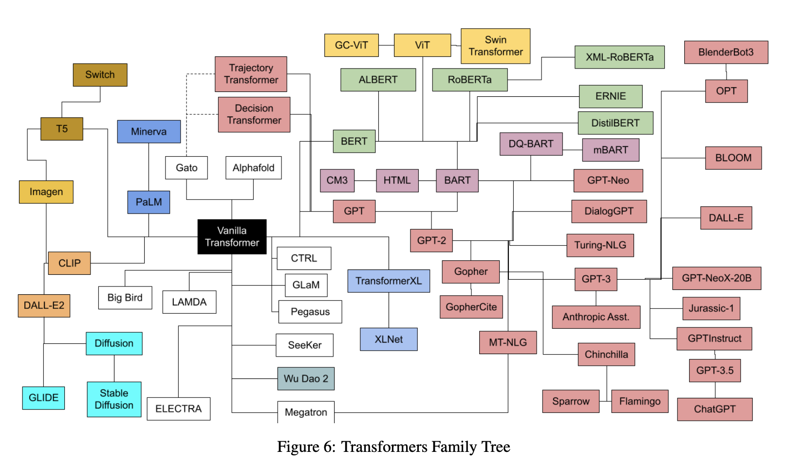
- Today, transformers are not just limited to language tasks but are used in vision, speech, and so much more. The following plot (source) shows the transformers family tree with prevalent models:
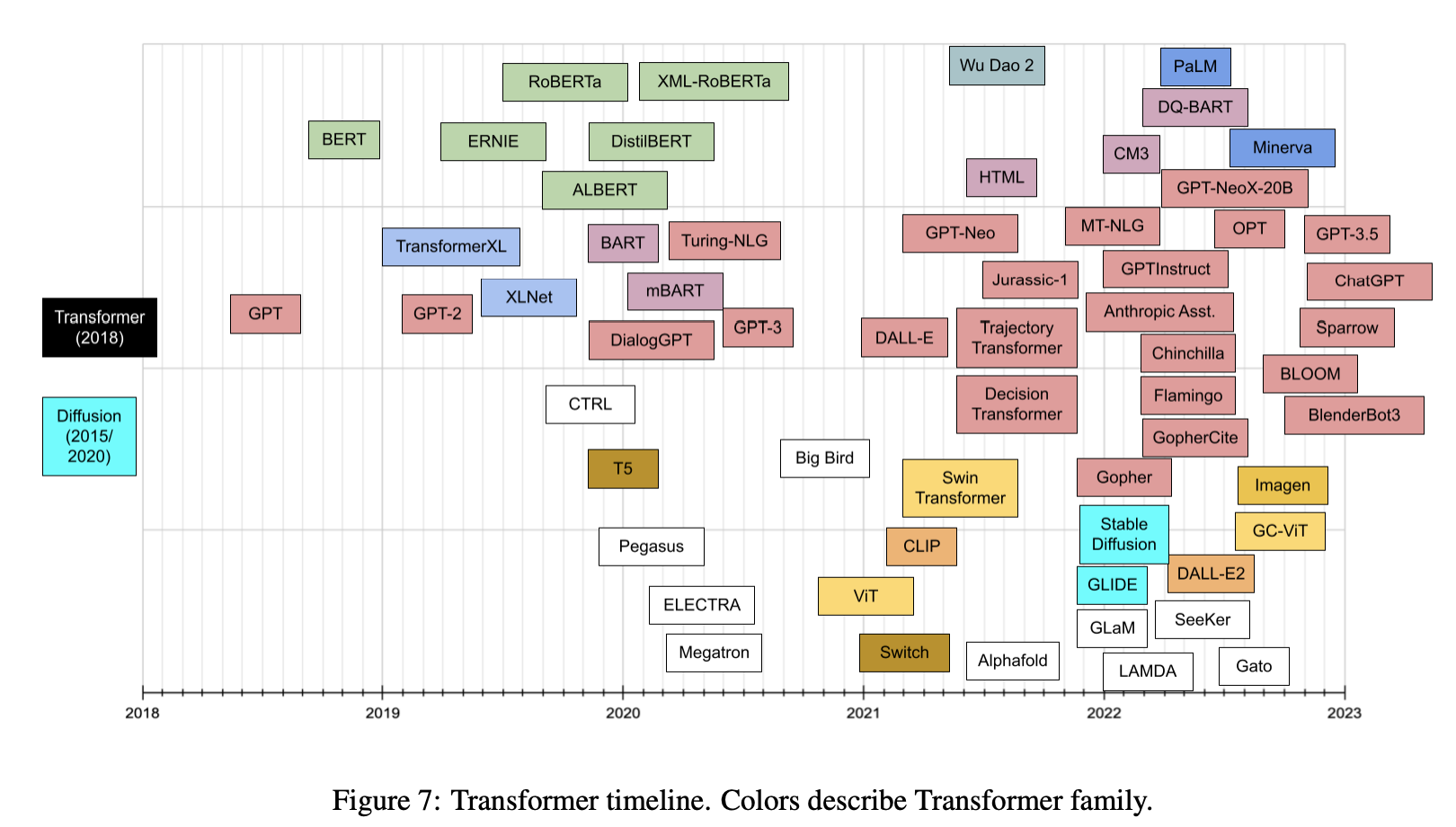
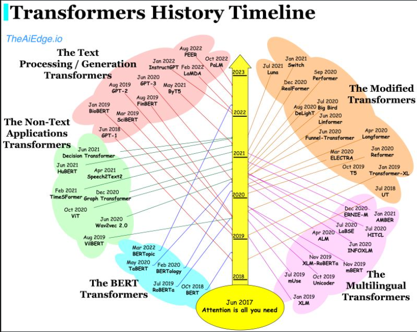
- And, the plots below (first plot source); (second plot source) show the timeline for prevalent transformer models:
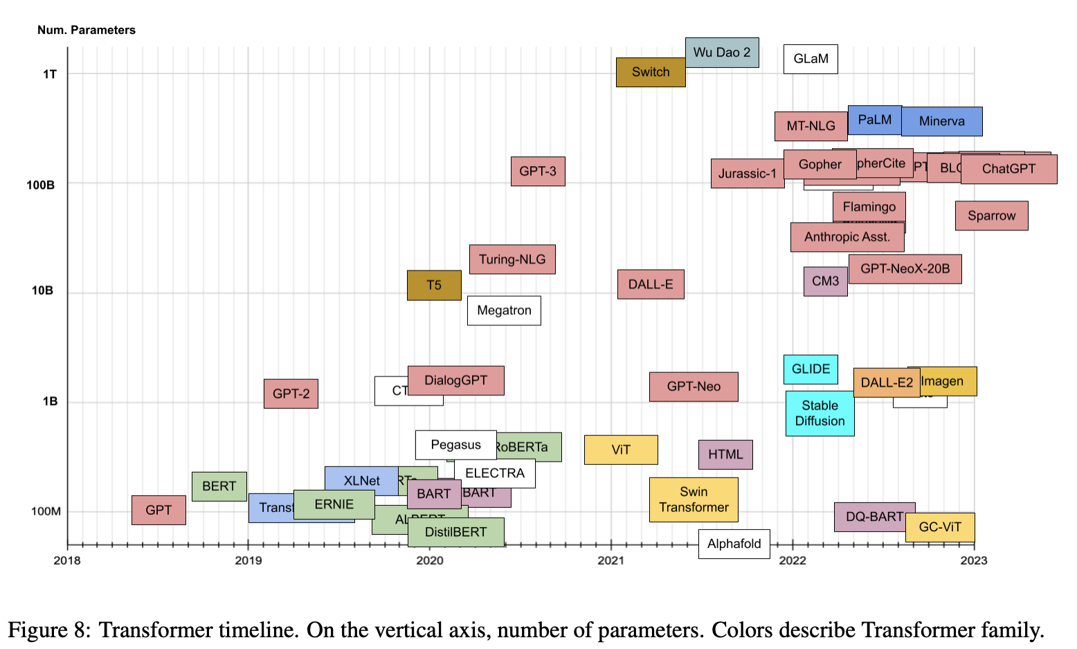
- Lastly, the plot below (source) shows the timeline vs. number of parameters for prevalent transformer models:
Transformers vs. Recurrent and Convolutional Architectures: An Overview
Language
- In a vanilla language model, for example, nearby words would first get grouped together. The transformer, by contrast, runs processes so that every element in the input data connects, or pays attention, to every other element. This is referred to as “self-attention.” This means that as soon as it starts training, the transformer can see traces of the entire data set.
- Before transformers came along, progress on AI language tasks largely lagged behind developments in other areas. Infact, in this deep learning revolution that happened in the past 10 years or so, natural language processing was a latecomer and NLP was, in a sense, behind computer vision, per the computer scientist Anna Rumshisky of the University of Massachusetts, Lowell.
- However, with the arrival of Transformers, the field of NLP has received a much-needed push and has churned model after model that have beat the state-of-the-art in various NLP tasks.
- As an example, to understand the difference between vanilla language models (based on say, a recurrent architecture such as RNNs, LSTMs or GRUs) vs. transformers, consider these sentences: “The owl spied a squirrel. It tried to grab it with its talons but only got the end of its tail.” The structure of the second sentence is confusing: What do those “it”s refer to? A vanilla language model that focuses only on the words immediately around the “it”s would struggle, but a transformer connecting every word to every other word could discern that the owl did the grabbing, and the squirrel lost part of its tail.
Vision
In CNNs, you start off being very local and slowly get a global perspective. A CNN recognizes an image pixel by pixel, identifying features like edges, corners, or lines by building its way up from the local to the global. But in transformers, owing to self-attention, even the very first attention layer models global contextual information, making connections between distant image locations (just as with language). If we model a CNN’s approach as starting at a single pixel and zooming out, a transformer slowly brings the whole fuzzy image into focus.
- CNNs work by repeatedly applying filters on local patches of the input data, generating local feature representations (or “feature maps”) and incrementally increase their receptive field and build up to global feature representations. It is because of convolutions that photo apps can organize your library by faces or tell an avocado apart from a cloud. Prior to the transformer architecture, CNNs were thus considered indispensable to vision tasks.
- With the Vision Transformer (ViT), the architecture of the model is nearly identical to that of the first transformer proposed in 2017, with only minor changes allowing it to analyze images instead of words. Since language tends to be discrete, a lot of adaptations were to discretize the input image to make transformers work with visual input. Exactly mimicing the language approach and performing self-attention on every pixel would be prohibitively expensive in computing time. Instead, ViT divides the larger image into square units, or patches (akin to tokens in NLP). The size is arbitrary, as the tokens could be made larger or smaller depending on the resolution of the original image (the default is 16x16 pixels). But by processing pixels in groups, and applying self-attention to each, the ViT could quickly churn through enormous training data sets, spitting out increasingly accurate classifications.
- In Do Vision Transformers See Like Convolutional Neural Networks?, Raghu et al. sought to understand how self-attention powers transformers in vision-based tasks.
Multimodal Tasks
- As discussed in the Enter the Transformer section, other architectures are “one trick ponies” while multimodal learning requires handling of modalities with different patterns within a streamlined architecture with a reasonably high relational inductive bias to even remotely reach human-like intelligence. In other words, we needs a single versatile architecture that seamlessly transitions between senses like reading/seeing, speaking, and listening.
- The potential to offer a universal architecture that can be adopted for multimodal tasks (that requires simultaneously handling multiple types of data, such as raw images, video and language) is something that makes the transformer architecture unique and popular.
- Because of the siloed approach with earlier architectures where each type of data had its own specialized model, this was a difficult task to accomplish. However, transformers offer an easy way to combine multiple input sources. For example, multimodal networks might power a system that reads a person’s lips in addition to listening to their voice using rich representations of both language and image information.
- By using cross-attention, where the query vector originates from one source and the key and value vectors come from another, transformers become highly effective for multimodal learning.
- The transformer thus offers be a big step toward achieving a kind of “convergence” for neural net architectures, resulting in a universal approach to processing data from multiple modalities.
Breaking Down the Transformer
- Prior to delving into the internal mechanisms of the Transformer architecture by examining each of its constituent components in detail, it is essential to first establish a foundational understanding of several underlying mathematical and conceptual constructs. These include, but are not limited to, one-hot vectors, the dot product, matrix multiplication, embedding generation, and the attention mechanism.
Background
One-Hot Encoding
Overview
-
Digital computers are inherently designed to process numerical data. However, in most real-world scenarios, the input data encountered is not naturally numerical. For instance, images are represented by pixel intensity values, and speech signals are modeled as oscillograms or spectrograms. Therefore, the initial step in preparing such data for computational models, especially machine learning algorithms, is to convert non-numeric inputs—such as text—into a numerical format that can be subjected to mathematical operations.
-
One-hot encoding is a method that transforms categorical variables into a format suitable for machine learning algorithms to enhance their predictive performance. Specifically, it converts categorical data into a binary matrix that enables the model to interpret each category as a distinct and independent feature.
Conceptual Intuition
- As one begins to work with machine learning models, the term “one-hot encoding” frequently arises. For example, in the scikit-learn documentation, one-hot encoding is described as a technique to “encode categorical integer features using a one-hot aka one-of-K scheme.” To elucidate this concept, let us consider a concrete example.
Example: Basic Dataset
- Consider the following illustrative dataset:
| CompanyName | CategoricalValue | Price |
|---|---|---|
| VW | 1 | 20000 |
| Acura | 2 | 10011 |
| Honda | 3 | 50000 |
| Honda | 3 | 10000 |
-
In this example, the column CategoricalValue represents a numerical label associated with each unique categorical entry (i.e., company names). If an additional company were to be included, it would be assigned the next incremental value, such as 4. Thus, as the number of distinct entries increases, so too does the range of the categorical labels.
-
It is important to note that the above table is a simplified representation. In practice, categorical values are typically indexed from 0 to \(N - 1\), where \(N\) is the number of distinct categories.
-
The assignment of categorical labels can be efficiently performed using the
LabelEncoderprovided by thesklearnlibrary. -
Returning to one-hot encoding: by adhering to the procedures outlined in the
sklearndocumentation and conducting minor data preprocessing, we can transform the previous dataset into the following format, wherein a value of1denotes presence and0denotes absence:
| VW | Acura | Honda | Price |
|---|---|---|---|
| 1 | 0 | 0 | 20000 |
| 0 | 1 | 0 | 10011 |
| 0 | 0 | 1 | 50000 |
| 0 | 0 | 1 | 10000 |
-
At this point, it is worth contemplating why mere label encoding might be insufficient when training machine learning models. Why is one-hot encoding preferred?
-
The limitation of label encoding lies in its implicit assumption of ordinal relationships among categories. For example, it inadvertently introduces a false hierarchy by implying
VW > Acura > Hondadue to their numeric encodings. If the model internally computes an average or distance metric over such values, the result could be misleading. Consider:(1 + 3)/2 = 2, which incorrectly suggests that the average of VW and Honda is Acura. Such outcomes undermine the model’s predictive accuracy and can lead to erroneous inferences. -
Therefore, one-hot encoding is employed to mitigate this issue. It effectively “binarizes” the categorical variable, enabling each category to be treated as an independent and mutually exclusive feature.
-
As a further example, suppose there exists a categorical feature named
flower, which can take the valuesdaffodil,lily, androse. One-hot encoding transforms this feature into three distinct binary features:is_daffodil,is_lily, andis_rose.
Example: Natural Language Processing
-
Drawing inspiration from Brandon Rohrer’s “Transformers From Scratch”, let us consider another illustrative scenario within the domain of natural language processing. Imagine we are designing a machine translation system that converts textual commands from one language to another. Such a model would receive a sequence of sounds and produce a corresponding sequence of words.
-
The first step involves defining the vocabulary—the set of all symbols that may appear in any input or output sequence. For this task, we would require two separate vocabularies: one representing input sounds and the other for output words.
-
Assuming we are working in English, the vocabulary could easily span tens of thousands of words, with additional entries to capture domain-specific jargon. This would result in a vocabulary size approaching one hundred thousand.
-
One straightforward method to convert words to numbers is to assign each word a unique integer ID. For instance, if our vocabulary consists of only three words—
files,find, andmy—we might map them as follows:files = 1,find = 2, andmy = 3. The phrase “Find my files” then becomes the sequence[2, 3, 1]. -
While this method is valid, an alternative representation that is more computationally favorable is one-hot encoding. In this approach, each word is encoded as a binary vector of length equal to the vocabulary size, where all elements are
0except for a single1at the index corresponding to the word. -
In other words, each word is still assigned a unique number, but now this number serves as an index in a binary vector. Using our earlier vocabulary, the phrase “find my files” can be encoded as follows:

- Thus, the sentence becomes a sequence of one-dimensional arrays (i.e., vectors), which, when concatenated, forms a two-dimensional matrix:

- It is pertinent to note that in this primer and many other contexts, the terms “one-dimensional array” and “vector” are used interchangeably. Likewise, “two-dimensional array” and “matrix” may be treated synonymously.
Dot product
- One really useful thing about the one-hot representation is that it lets us compute dot product (also referred to as the inner product, scalar product or cosine similarity).
Algebraic Definition
-
The dot product of two vectors \(\mathbf{a}=\left[a_{1}, a_{2}, \ldots, a_{n}\right]\) and \(\mathbf{b}=\left[b_{1}, b_{2}, \ldots, b_{n}\right]\) is defined as:
\[\mathbf{a} \cdot \mathbf{b}=\sum_{i=1}^{n} a_{i} b_{i}=a_{1} b_{1}+a_{2} b_{2}+\cdots+a_{n} b_{n}\]- where \(\Sigma\) denotes summation and \(n\) is the dimension of the vector space.
-
For instance, in three-dimensional space, the dot product of vectors \([1, 3, -5]\) and \([4,-2,-1]\) is:
\[\begin{aligned} {[1,3,-5] \cdot[4,-2,-1] } &=(1 \times 4)+(3 \times-2)+(-5 \times-1) \\ &=4-6+5 \\ &=3 \end{aligned}\] -
The dot product can also be written as a product of two vectors, as below.
\[\mathbf{a} \cdot \mathbf{b}=\mathbf{a b}^{\top}\]- where \(\mathbf{b}^{\top}\) denotes the transpose of \(\mathbf{b}\).
-
Expressing the above example in this way, a \(1 \times 3\) matrix (row vector) is multiplied by a \(3 \times 1\) matrix (column vector) to get a \(1 \times 1\) matrix that is identified with its unique entry:
\[\left[\begin{array}{lll} 1 & 3 & -5 \end{array}\right]\left[\begin{array}{c} 4 \\ -2 \\ -1 \end{array}\right]=3\] -
Key takeaway:
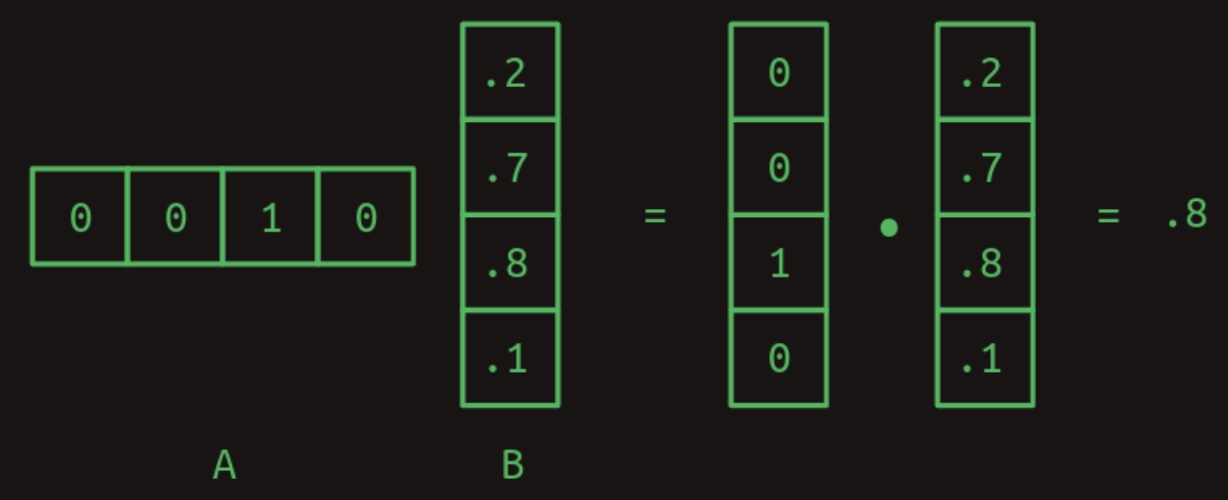
- In summary, to get the dot product of two vectors, multiply their corresponding elements, then add the results. For a visual example of calculating the dot product for two vectors, check out the figure below.

Geometric Definition
-
In Euclidean space, a Euclidean vector is a geometric object that possesses both a magnitude and a direction. A vector can be pictured as an arrow. Its magnitude is its length, and its direction is the direction to which the arrow points. The magnitude of a vector a is denoted by \(\mid \mid a \mid \mid\). The dot product of two Euclidean vectors \(\mathbf{a}\) and \(\mathbf{b}\) is defined by,
\[\mathbf{a} \cdot \mathbf{b}=\mid \mathbf{a}\mid \mid \mathbf{b}\mid \cos \theta\]- where \(\theta\) is the angle between \(\mathbf{a}\) and \(\mathbf{b}\).
-
The above equation establishes the relation between dot product and cosine similarity.
Properties of the dot product
-
Dot products are especially useful when we’re working with our one-hot word representations owing to it’s properties, some of which are highlighted below.
-
The dot product of any one-hot vector with itself is one.

- The dot product of any one-hot vector with another one-hot vector is zero.

- The previous two examples show how dot products can be used to measure similarity. As another example, consider a vector of values that represents a combination of words with varying weights. A one-hot encoded word can be compared against it with the dot product to show how strongly that word is represented. The following figure shows how a similarity score between two vectors is calculated by way of calculating the dot product.

Matrix Multiplication as a Series of Dot Products
- The dot product constitutes the fundamental operation underlying matrix multiplication, which is a highly structured and well-defined procedure for combining two two-dimensional arrays (matrices). Let us denote the first matrix by \(A\) and the second by \(B\). In the most elementary scenario, where \(A\) consists of a single row and \(B\) consists of a single column, the matrix multiplication reduces to the dot product of these two vectors. This is illustrated in the figure below:
-
Observe that for this operation to be well-defined, the number of columns in matrix \(A\) must be equal to the number of rows in matrix \(B\). This dimensional compatibility is a prerequisite for the dot product to be computable.
-
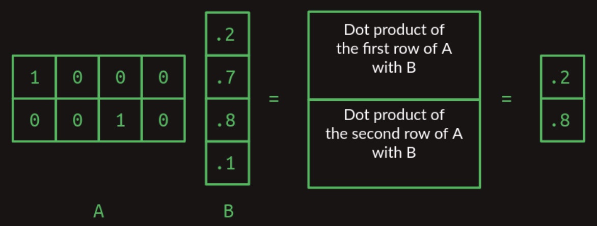
As the dimensions of matrices \(A\) and \(B\) increase, the computational complexity of matrix multiplication grows accordingly—specifically, in a quadratic manner with respect to the matrix dimensions. When matrix \(A\) contains multiple rows, the multiplication proceeds by computing the dot product between each row of \(A\) and the entire matrix \(B\). Each such operation produces a single scalar value, and the collection of these values forms a resulting matrix with the same number of rows as \(A\). This process is depicted in the following figure, which shows the multiplication of a two-row matrix and a single-column matrix:
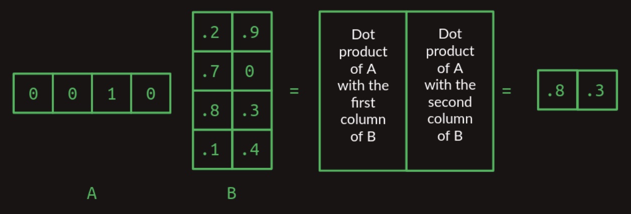
- If matrix \(B\) possesses more than one column, the operation is generalized by taking the dot product of each row in \(A\) with each column in \(B\). The outcome of each row-column dot product populates the corresponding cell in the resultant matrix. The figure below demonstrates the multiplication of a one-row matrix with a two-column matrix:
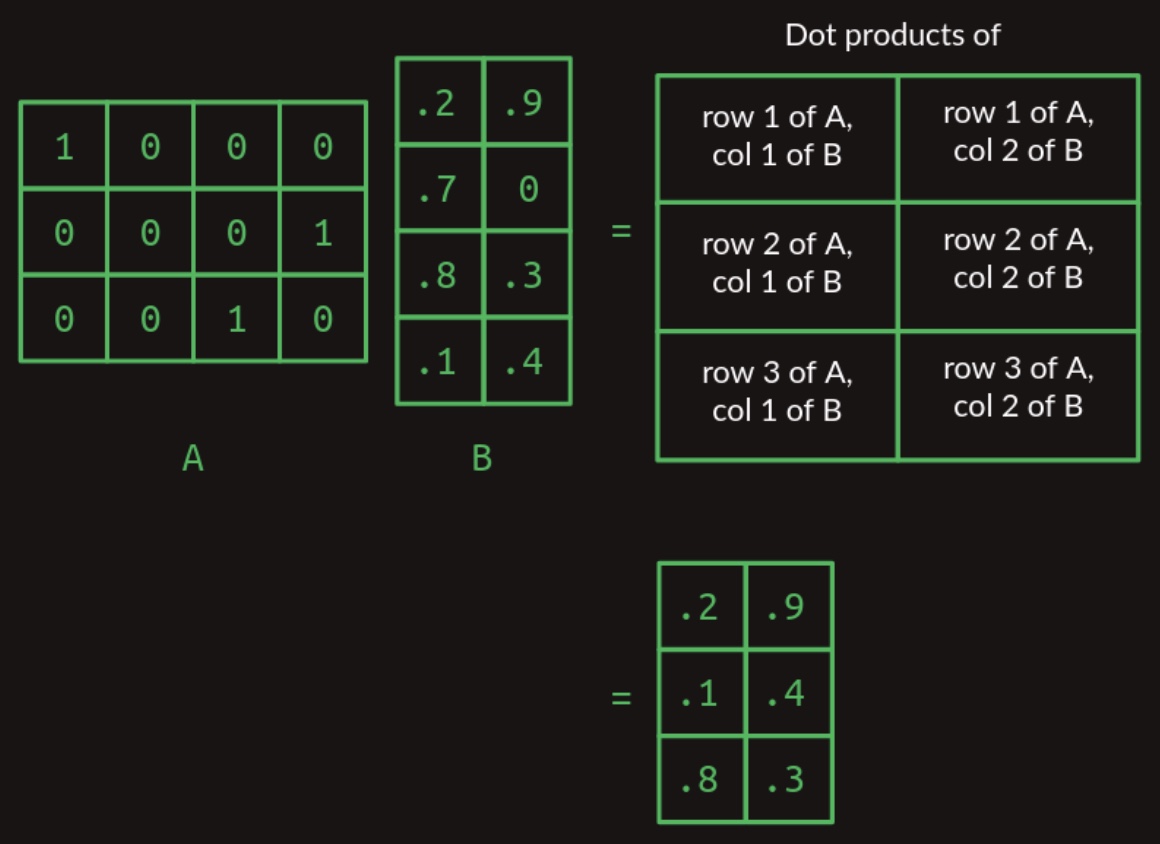
- Building on these principles, we can now define the general case of matrix multiplication for two arbitrary matrices, provided that the number of columns in matrix \(A\) equals the number of rows in matrix \(B\). The resultant matrix will have a shape defined by the number of rows in \(A\) and the number of columns in \(B\). This general case is visualized in the figure below, which illustrates the multiplication of a one-by-three matrix with a two-column matrix:
Matrix Multiplication as a Table Lookup
-
In the preceding section, we examined how matrix multiplication can function as a form of table lookup.
-
Consider a matrix \(A\) composed of a stack of one-hot encoded vectors. For the sake of illustration, suppose these vectors have non-zero entries (i.e., ones) located in the first column, fourth column, and third column, respectively. During matrix multiplication with another matrix \(B\), these one-hot vectors act as selection mechanisms that extract the corresponding rows—specifically, the first, fourth, and third rows—from matrix \(B\), in that order.
-
This method of employing a one-hot vector to selectively retrieve a specific row from a matrix lies at the conceptual foundation of the Transformer architecture. It enables discrete, deterministic access to embedding representations or other learned vector structures by treating the multiplication as a row-indexing operation.
First-Order Sequence Model
-
Let us momentarily set aside matrices and return our focus to sequences of words, which are the primary objects of interest in natural language processing.
-
Suppose we are developing a rudimentary natural language interface for a computer system, and initially, we aim to accommodate only three predefined command phrases:
Show me my directories please.
Show me my files please.
Show me my photos please.
- Given these sample utterances, our working vocabulary consists of the following seven distinct words:
{directories, files, me, my, photos, please, show}
-
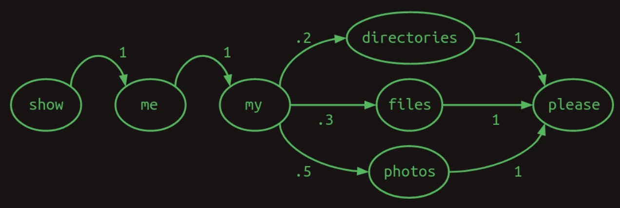
One effective way to represent such sequences is through the use of a transition model, which encapsulates the probabilistic dependencies between successive words. For each word in the vocabulary, the model estimates the likelihood of possible subsequent words. For instance, if users refer to photos 50% of the time, files 30% of the time, and directories 20% of the time following the word “my”, these probabilities define a distribution over transitions from “my”.
-
Importantly, the transition probabilities originating from any given word must collectively sum to one, reflecting a complete probability distribution over the vocabulary. The following diagram illustrates this concept in the form of a Markov chain:
-
This specific type of transition model is referred to as a Markov chain, as it satisfies the Markov property: the probability of transitioning to the next word depends only on a limited number of prior states. More precisely, this is a first-order Markov model, meaning that the next word is conditioned only on the immediately preceding word. If the model instead considered the two most recent words, it would be categorized as a second-order Markov model.
-
We now return to matrices, which offer a convenient and compact representation of such probabilistic transition systems. The Markov chain can be encoded as a transition matrix, where each row and column corresponds to a unique word in the vocabulary, indexed identically to their respective positions in the one-hot encoding.
-
The transition matrix can thus be interpreted as a lookup table. Each row represents a starting word, and the values in that row’s columns indicate the probabilities of each word in the vocabulary occurring next. Because these values represent probabilities, they all lie in the interval \([0, 1]\), and the entries in each row collectively sum to 1.
-
The diagram below, adapted from Brandon Rohrer’s “Transformers From Scratch”, illustrates such a transition matrix:

-
Within this matrix, the structure of the three example sentences is clearly discernible. The vast majority of the transition probabilities are binary (i.e., either 0 or 1), indicating deterministic transitions. The only point of stochasticity arises after the word “my,” where the model branches probabilistically to either “directories,” “files,” or “photos.” Outside of this branching, the sequence progression is entirely deterministic, and this is reflected by the predominance of ones and zeros in the matrix.
-
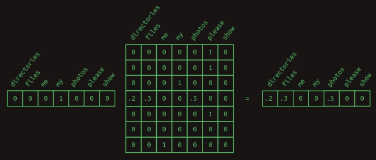
We now revisit the earlier technique of matrix-vector multiplication for efficient retrieval. Specifically, we can multiply a one-hot vector—representing a given word—with the transition matrix to extract the associated row, which contains the conditional probability distribution for the next word. For example, to determine the distribution over words that follow “my,” we construct a one-hot vector for “my” and multiply it with the transition matrix. This operation retrieves the relevant row and thus reveals the desired transition probabilities.
-
The following figure, also from Brandon Rohrer’s “Transformers From Scratch”, visualizes this operation:
Second-Order Sequence Model
-
Predicting the next word in a sequence based solely on the current word is inherently limited. It is akin to attempting to predict the remainder of a musical composition after hearing only the initial note. The likelihood of accurate prediction improves significantly when at least two preceding words are taken into account.
-
This improvement is demonstrated using a simplified language model tailored for basic computer commands. Suppose the model is trained to recognize only the following two sentences, occurring in a \(\frac{40}{60}\) ratio, respectively:
Check whether the battery ran down please.
Check whether the program ran please.
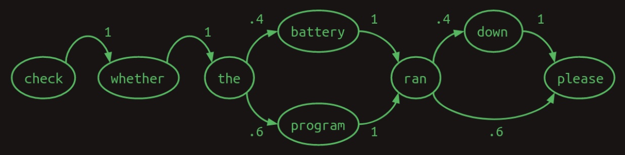
- A first-order Markov chain—where the next word depends only on the immediately preceding word—can model this system. The diagram below, sourced from Brandon Rohrer’s Transformers From Scratch, illustrates the first-order transition structure:
-
However, this model exhibits limitations. If the model considers not just one but the two most recent words, its predictive accuracy improves. For instance, when it encounters the phrase
battery ran, it can confidently predict that the next word isdown. Conversely,program ranleads unambiguously toplease. Incorporating the second-most-recent word eliminates branching ambiguity, reduces uncertainty, and enhances model confidence. -
Such a system is known as a second-order Markov model, as it uses two previous states (words) to predict the next. While second-order chains are more difficult to visualize, the underlying connections offer greater predictive power. The diagram below, again from Brandon Rohrer’s Transformers From Scratch, illustrates this structure:

-
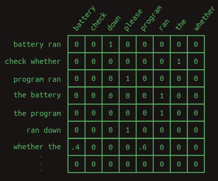
To emphasize the contrast, consider the following two transition matrices:
- First-order transition matrix:
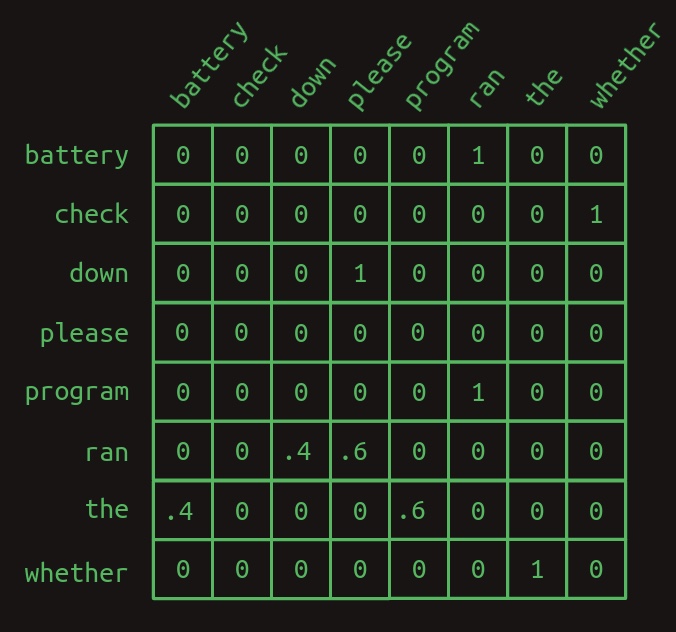
- Second-order transition matrix:
-
In the second-order matrix, each row corresponds to a unique combination of two words, representing context for predicting the next word. Consequently, with a vocabulary size of \(N\), the matrix will contain \(N^2\) rows.
-
The advantage of this structure is increased certainty. The second-order matrix contains more entries with a value of 1 and fewer fractional probabilities, indicating a more deterministic model. Only a single row contains fractional values—highlighting the only point of uncertainty in the model. Intuitively, incorporating two words rather than one provides additional context, thereby enhancing the reliability of next-word predictions.
Second-Order Sequence Model with Skips
- A second-order model is effective when the word immediately following depends primarily on the two most recent words. However, complications arise when longer-range dependencies are necessary. Consider the following pair of equally likely sentences:
Check the program log and find out whether it ran please.
Check the battery log and find out whether it ran down please.
-
In this case, to accurately predict the word following
ran, one would need to reference context extending up to eight words into the past. One potential solution is to adopt a higher-order Markov model, such as a third-, fourth-, or even eighth-order model. However, this approach becomes computationally intractable: a naive implementation of an eighth-order model would necessitate a transition matrix with \(N^8\) rows, which is prohibitively large for realistic vocabulary sizes. -
An alternative strategy is to preserve a second-order model while allowing for non-contiguous dependencies. Specifically, the model considers the combination of the most recent word with any previously seen word in the sequence. Although each prediction still relies on just two words, the approach enables the model to capture long-range dependencies.
-
This technique, often termed second-order with skips, differs from full higher-order models in that it disregards much of the sequential ordering and only retains select pairwise interactions. Nevertheless, it remains effective for sequence modeling in many practical cases.
-
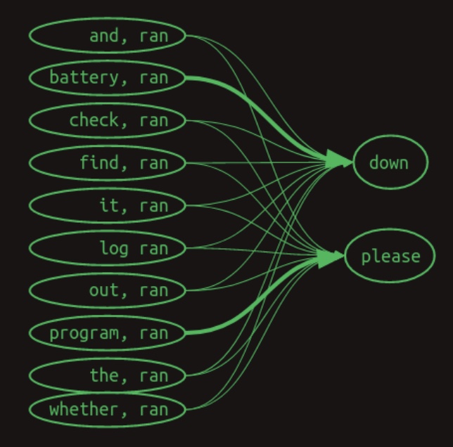
At this point, classical Markov chains are no longer applicable. Instead, the model tracks associative links between earlier words and subsequent words, regardless of strict temporal adjacency. The diagram below from Brandon Rohrer’s Transformers From Scratch visualizes these interactions using directional arrows. Numeric weights are omitted; instead, line thickness indicates the strength of association:
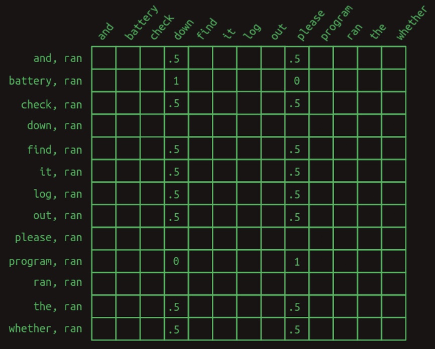
- The corresponding transition matrix for this second-order-with-skips model is shown below:
-
This matrix view is restricted to the rows pertinent to predicting the word that follows
ran. Each row corresponds to a pair consisting ofranand another word in the vocabulary. Only non-zero entries are shown; cells not displayed are implicitly zero. -
The first key insight is that, in this model, prediction is based not on a single row but on a collection of rows—each representing a feature defined by a specific word pair. Consequently, we move beyond traditional Markov chains. Rows no longer represent the complete state of a sequence, but instead denote individual contextual features active at a specific moment.
-
As a result of this shift, each value in the matrix is no longer interpreted as a probability, but rather as a vote. When predicting the next word, votes from all active features are aggregated, and the word receiving the highest cumulative score is selected.
-
The second key observation is that most features have little discriminatory power. Since the majority of words appear in both sentences, their presence does not help disambiguate what comes after
ran. These features contribute uniformly with a value of 0.5, offering no directional influence. -
The only features with predictive utility in this example are
battery, ranandprogram, ran. The featurebattery, ranimplies thatranis the most recent word andbatteryoccurred earlier. This feature assigns a vote of 1 todownand 0 toplease. Conversely,program, ranassigns the inverse: a vote of 1 topleaseand 0 todown. -
To generate a next-word prediction, the model sums all applicable feature values column-wise. For instance:
- In the sequence
Check the program log and find out whether it ran, the cumulative votes are 0 for most words, 4 fordown, and 5 forplease. - In the sequence
Check the battery log and find out whether it ran, the votes are reversed: 5 fordownand 4 forplease.
- In the sequence
-
By selecting the word with the highest vote total, the model makes the correct next-word prediction—even when the relevant information is located eight words earlier. This highlights the utility and efficiency of feature-based second-order-with-skips models in capturing long-range dependencies without incurring the exponential complexity of full higher-order Markov models.
Masking Features
-
Upon closer examination, the predictive difference between vote totals of 4 and 5 is relatively minor. Such a narrow margin indicates that the model lacks strong confidence in its prediction. In larger and more naturalistic language models, these subtle distinctions are likely to be obscured by statistical noise, potentially leading to inaccurate or unstable predictions.
-
One effective strategy to sharpen predictions is to eliminate the influence of uninformative features. In the given example, only two features—
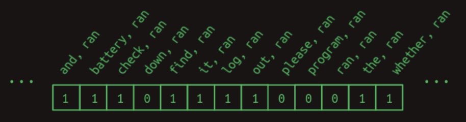
battery, ranandprogram, ran—meaningfully contribute to next-word prediction. It is instructive at this point to recall that relevant rows are extracted from the transition matrix via a dot product between the matrix and a feature activity vector, which encodes the features currently active. For this scenario, the implicitly used feature vector is visualized in the following diagram from Brandon Rohrer’s Transformers From Scratch:
-
This vector includes an entry with the value 1 for each feature formed by pairing
ranwith each preceding word in the sentence. Notably, words that occur afterranare excluded, as in the next-word prediction task these words remain unseen at prediction time and therefore must not influence the outcome. Moreover, combinations that do not arise in the example context are safely assumed to yield zero values and can be ignored without loss of generality. -
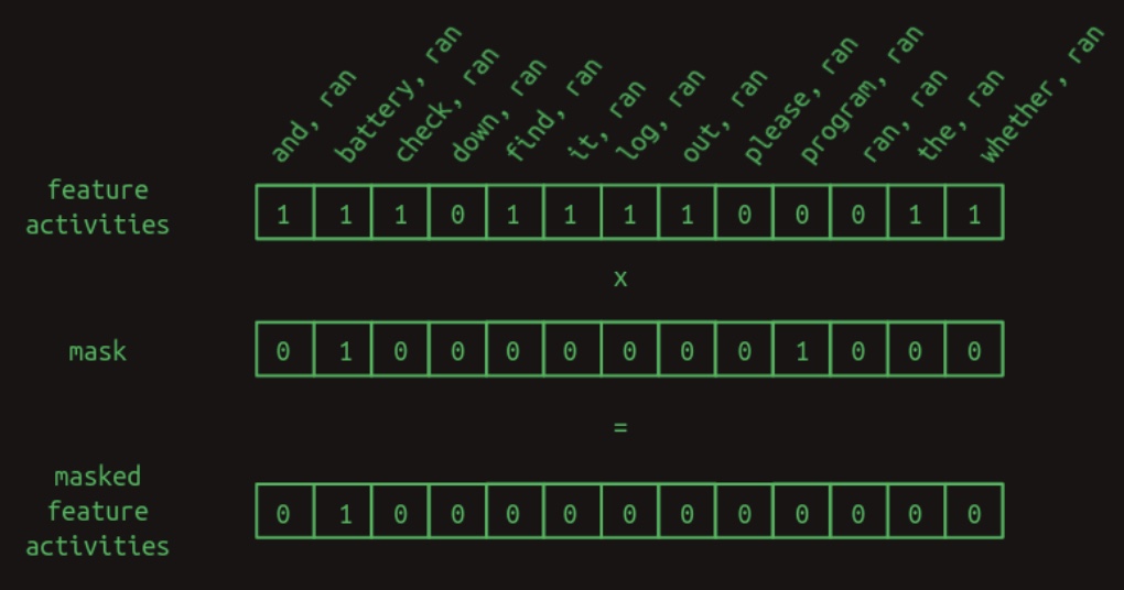
To enhance model precision further, we can introduce a masking mechanism that explicitly nullifies unhelpful features. A mask is defined as a binary vector, populated with ones at positions corresponding to features we wish to retain, and zeros at positions to be suppressed or ignored. In this case, we wish to retain only
battery, ranandprogram, ran, the features that empirically prove to be informative. The masked feature vector is illustrated in the diagram below, also from Brandon Rohrer’s Transformers From Scratch:
-
The mask is applied to the original feature activity vector via element-wise multiplication. For any feature retained by the mask (i.e., mask value of 1), its corresponding activity remains unchanged. Conversely, features masked out (i.e., mask value of 0) are forcibly zeroed out, regardless of their original value.
-
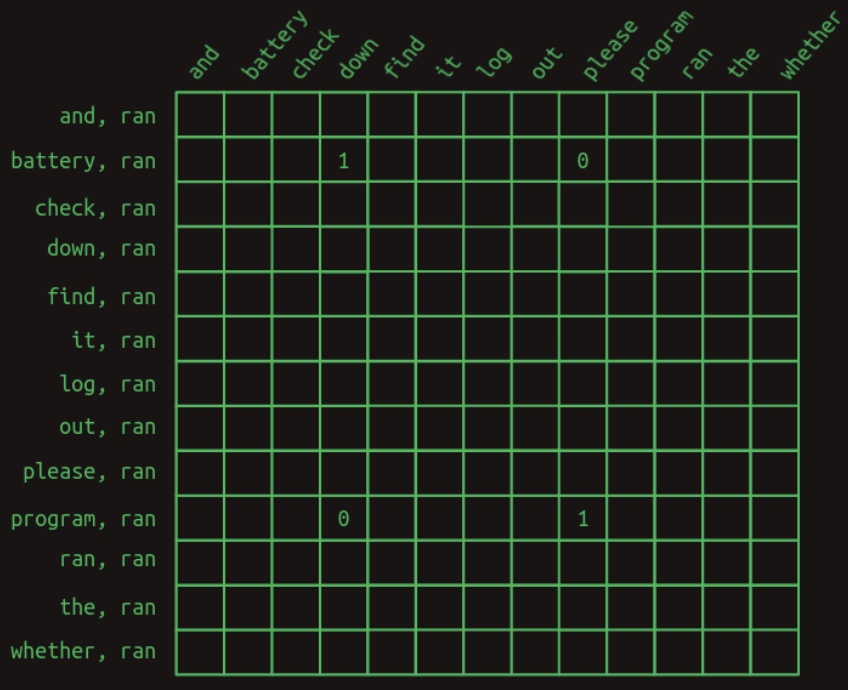
The practical effect of the mask is that large portions of the transition matrix are suppressed. All feature combinations of
ranwith any word other thanbatteryorprogramare effectively removed from consideration. The resultant masked transition matrix is shown below:
-
Once uninformative features are masked out, the model’s predictive power becomes significantly stronger. For instance, when the word
batteryappears earlier in the sequence, the model now assigns a probability weight of 1 todownand 0 topleasefor the next word followingran. What was previously a 25% difference in weighting has now become an unambiguous selection, or informally, an “infinite percent” improvement in certainty. A similar confidence gain is observed when the wordprogramappears earlier, resulting in a decisive preference forplease. -
This process of selective masking is a core conceptual component of the attention mechanism, as referenced in the title of the original Transformer paper. While the simplified mechanism described here provides an intuitive foundation, the actual implementation of attention in Transformers is more sophisticated. For a comprehensive treatment, refer to the original paper.
Generally speaking, an attention function determines the relative importance (or “weight”) of different input elements in producing an output representation. In the specific case of scaled dot-product attention, which the Transformer architecture employs, the mechanism adopts the query-key-value paradigm from information retrieval. An attention function performs a mapping from a query and a set of key-value pairs to a single output. This output is computed as a weighted sum of the values, where each weight is derived from a compatibility function—also known as an alignment function, as introduced in Bahdanau et al. (2014)—which measures the similarity between the query and each key.
- This overview introduces the fundamental principles of attention. The specific computational details and extensions, including multi-head attention and positional encoding, are addressed in the dedicated section on Attention.
Origins of attention
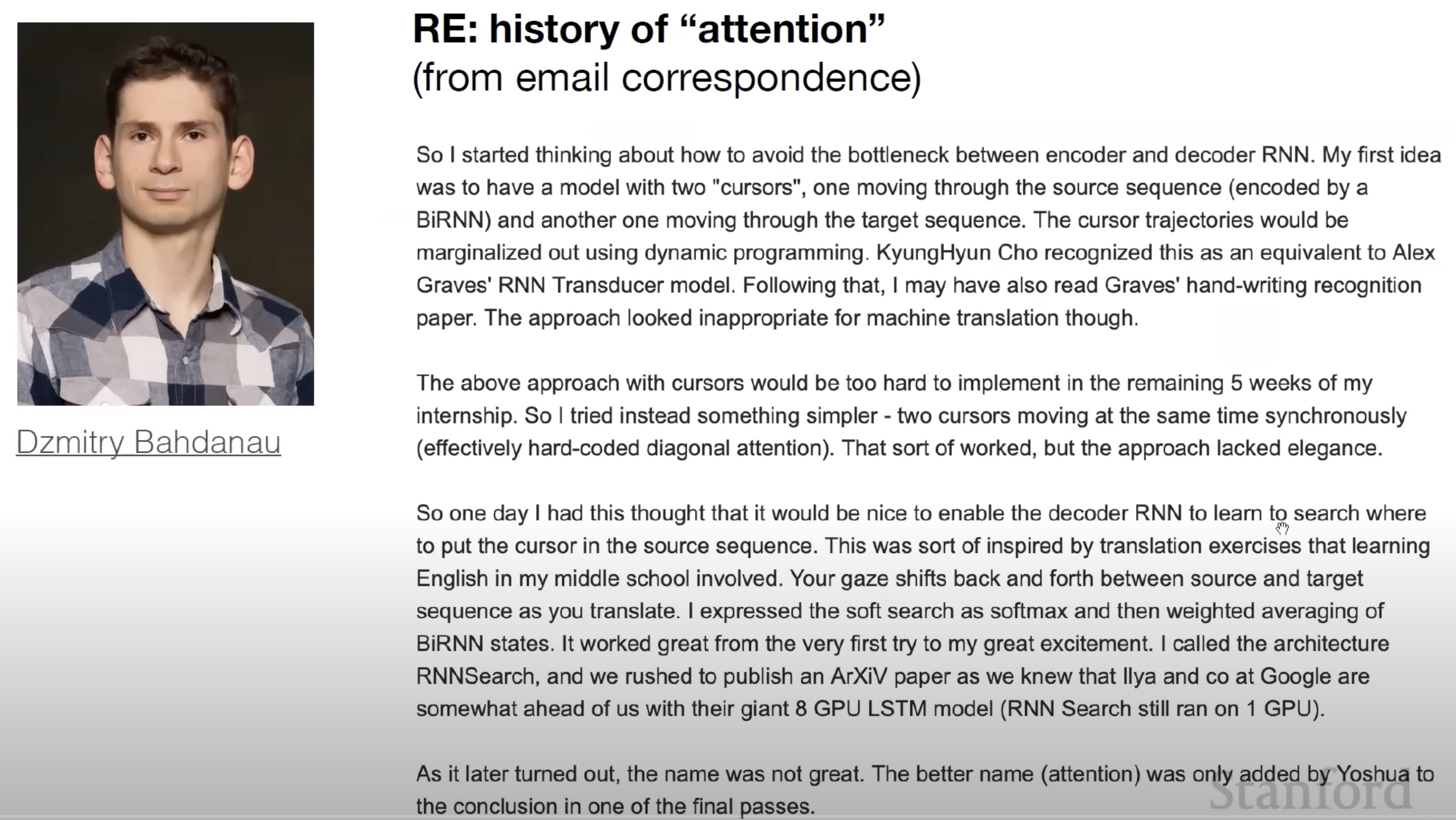
- As mentioned above, the attention mechanism originally introduced in Bahdanau et al. (2015) served as a foundation upon which the self-attention mechanism in the Transformer paper was based on.
- The following slide from Stanford’s CS25 course shows how the attention mechanism was conceived and is a perfect illustration of why AI/ML is an empirical field, built on intuition.
From Feature Vectors to Transformers
-
The selective-second-order-with-skips model provides a valuable conceptual framework for understanding the operations of Transformer-based architectures, particularly on the decoder side. It serves as a reasonable first-order approximation of the underlying mechanics in generative language models such as OpenAI’s GPT-3. Although it does not fully encompass the complexity of Transformer models, it encapsulates the core intuition that drives them.
-
The subsequent sections aim to bridge the gap between this high-level conceptualization and the actual computational implementations of Transformers. The evolution from intuition to implementation is primarily shaped by three key practical considerations:
-
Computational efficiency of matrix multiplications Modern computers are exceptionally optimized for performing matrix multiplications. In fact, an entire industry has emerged around designing hardware tailored for this specific operation. Central Processing Units (CPUs) handle matrix multiplications effectively due to their ability to leverage multi-threading. Graphics Processing Units (GPUs), however, are even more efficient, as they contain hundreds or thousands of dedicated cores optimized for highly parallelized computations. Consequently, any algorithm or computation that can be reformulated as a matrix multiplication can be executed with remarkable speed and efficiency. This efficiency has led to the analogy: matrix multiplication is like a bullet train—if your data (or “baggage”) can be expressed in its format, it will reach its destination extremely quickly.
-
Differentiability of every computational step Thus far, our examples have involved manually defined transition probabilities and masking patterns—effectively, manually specified model parameters. In practical settings, however, these parameters must be learned from data using the process of backpropagation. For backpropagation to function, each computational operation in the network must be differentiable. This means that any infinitesimal change in a parameter must yield a corresponding, computable change in the model’s loss function—the measure of error between predictions and target outputs.
-
Gradient smoothness and conditioning The loss gradient, which comprises the set of all partial derivatives with respect to the model’s parameters, must exhibit smoothness and favorable conditioning to ensure effective optimization. A smooth gradient implies that small parameter updates result in proportionally small and consistent changes in loss—facilitating stable convergence. A well-conditioned gradient further ensures that no direction in the parameter space dominates excessively over others. To illustrate: if the loss surface were analogous to a geographic landscape, then a well-conditioned loss would resemble gently rolling hills (as in the classic Windows screensaver), whereas a poorly conditioned loss would resemble the steep, asymmetrical cliffs of the Grand Canyon. In the latter case, optimization algorithms would struggle to find a consistent update direction due to varying gradients depending on orientation.
-
-
If we consider the science of neural network architecture to be about designing differentiable building blocks, then the art lies in composing these blocks such that the gradient is smooth and approximately uniform in all directions—ensuring robust training dynamics.
Attention as Matrix Multiplication
-
While it is relatively straightforward to assign feature weights by counting co-occurrences of word pairs and subsequent words during training, attention masks are not as trivially derived. Until now, mask vectors have been assumed or manually specified. However, within the Transformer architecture, the process of discovering relevant masks must be both automated and differentiable.
-
Although it might seem intuitive to use a lookup table for this purpose, the design imperative in Transformers is to express all major operations as matrix multiplications, for the reasons discussed above.
-
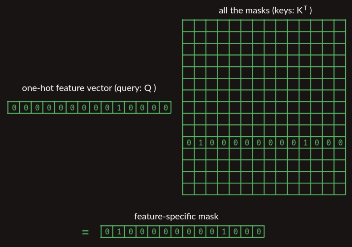
We can adapt the earlier lookup mechanism by aggregating all possible mask vectors into a matrix, and using the one-hot representation of the current word to extract the appropriate mask vector. This procedure is depicted in the diagram below:
-
For visual clarity, the diagram illustrates only the specific mask vector being accessed, though the full matrix contains one mask vector for each vocabulary entry.
-
This leads us into alignment with the formal Transformer architecture as described in the original paper. The mechanism for retrieving a relevant mask via matrix operations corresponds to the \(QK^T\) term in the attention equation, which is introduced in more detail in the section on Single Head Attention Revisited:
-
In this formulation:
- The matrix \(Q\) (queries) encodes the features we are currently focusing on.
- The matrix \(K\) (keys) stores the collection of masking vectors (or more broadly, content to be attended to).
- Since the keys are stored in columns, but queries are row vectors, the keys must be transposed (denoted by the \(T\) operator) to enable appropriate dot-product alignment.
-
The resulting dot product between the query and each key vector yields a compatibility score. This score is then scaled by \(\sqrt{d_k}\) (to stabilize gradients during training), and passed through a softmax function to convert it into a probability distribution over the values. Finally, this distribution is used to compute a weighted sum of the value vectors in \(V\).
-
While we will revisit and refine this formulation in upcoming sections, this abstraction already demonstrates the core idea: attention as differentiable lookup, implemented entirely through matrix operations.
-
Additional elaboration on this mechanism can be found in the section on Attention below.
Second-Order Sequence Model as Matrix Multiplications
-
One aspect we have thus far treated somewhat informally is the construction of transition matrices. While the logical structure and function of these matrices have been discussed, we have not yet fully articulated how to implement them using matrix multiplication, which is central to efficient neural network computation.
-
Once the attention step is complete, it produces a vector that represents the most recent word along with a small subset of previously encountered words. This attention output provides the raw material necessary for feature construction, but it does not directly generate the multi-word (word-pair) features required for downstream processing. To construct these features—combinations of the most recent word with one or more earlier words—we can employ a single-layer fully connected neural network.
-
To illustrate how such a neural network layer can perform this construction, we will design a hand-crafted example. While this example is intentionally stylized and its weight values do not reflect real-world training outcomes, it serves to demonstrate that a neural network possesses the expressive capacity required to form word-pair features. For clarity and conciseness, we will restrict the vocabulary to just three attended words:
battery,program, andran. The following diagram from Brandon Rohrer’s Transformers From Scratch shows a neural network layer designed to generate multi-word features:
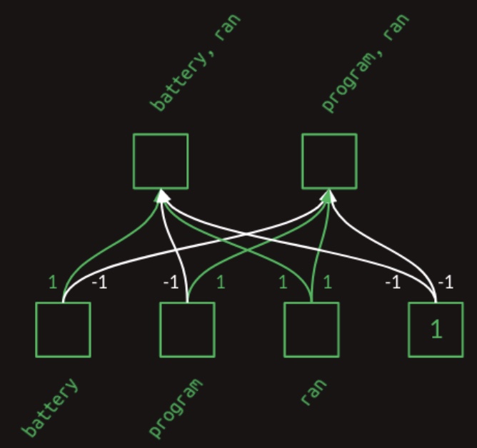
- The diagram illustrates how learned weights in the network can combine presence (indicated by a
1) and absence (indicated by a0) of words to produce a set of feature activations. This same transformation can also be expressed in matrix form. The following image depicts the weight matrix corresponding to this feature generation layer:

- Feature activations are computed by multiplying this weight matrix by a vector representing the current word context—that is, the presence or absence of each relevant word seen so far. The next diagram, also from Rohrer’s primer, illustrates this computation for the feature
battery, ran:

- In this instance, the vector has ones in the positions corresponding to
batteryandran, a zero forprogram, and a bias input fixed at one (a standard element in neural networks to allow shifting the activation). The result of the matrix multiplication yields a1for thebattery, ranfeature and-1forprogram, ran. This demonstrates how specific combinations of input activations result in distinct feature detections. The computation forprogram, ranproceeds analogously, as shown here:

-
The final step in constructing these features involves applying a Rectified Linear Unit (ReLU) non-linearity. The ReLU function replaces any negative values with zero, effectively acting as a thresholding mechanism that retains only positive activations. This ensures that features are expressed in binary form—indicating presence with a
1and absence with a0. -
With these steps complete, we now have a matrix-multiplication-based procedure for generating multi-word features. Although we initially described these as consisting solely of the most recent word and one preceding word, a closer examination reveals that this method is more general. When the feature generation matrix is learned (rather than hard-coded), the model is capable of representing more complex structures, including:
- Three-word combinations, such as
battery, program, ran, if they occur frequently enough during training. - Co-occurrence patterns that ignore the most recent word, such as
battery, program.
- Three-word combinations, such as
-
Such capabilities reveal that the model is not strictly limited to a selective-second-order-with-skips formulation, as previously implied. Rather, the actual representational capacity of Transformers extends beyond this simplification, capturing more nuanced and flexible feature structures. This additional complexity illustrates that our earlier model was a useful abstraction, but not a complete one—and that abstraction will continue to evolve as we explore further layers of the architecture.
-
Once generated, the multi-word feature matrix is ready to undergo one final matrix multiplication: the application of the second-order sequence model with skips, as introduced earlier. Altogether, the following sequence of feed-forward operations is applied after the attention mechanism:
- Feature creation via matrix multiplication
- Application of ReLU non-linearity
- Transition matrix multiplication
-
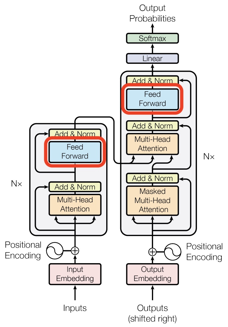
These operations correspond to the feed forward block in the Transformer architecture. The following equation from the original paper expresses this process concisely in mathematical terms:

- In the architectural diagram below, also from the Transformer paper, these operations are grouped together under the label feed forward:
Sampling a Sequence of Output Words
Generating Words as a Probability Distribution over the Vocabulary
-
Up to this point, our discussion has focused primarily on the task of next-word prediction. To extend this into the generation of entire sequences, such as complete sentences or paragraphs, several additional components must be introduced. One critical element is the prompt—a segment of initial text that provides the Transformer with contextual information and a starting point for further generation. This prompt serves as an input to the decoder, which corresponds to the right-hand side of the model architecture (as labeled “Outputs (shifted right)” in conventional visualizations).
-
The selection and design of a prompt that elicits meaningful or interesting responses from the model is a specialized practice known as prompt engineering. This emerging field exemplifies a broader trend in artificial intelligence where human users adapt their inputs to support algorithmic behavior, rather than expecting models to adapt to arbitrary human instructions.
-
During sequence generation, the decoder is typically initialized with a special token such as
<START>, which acts as a signal to commence decoding. This token enables the decoder to begin leveraging the compressed representation of the source input, as derived from the encoder (explored further in the section on Cross-Attention). The following animation from Jay Alammar’s The Illustrated Transformer illustrates two key processes:- Parallel ingestion of tokens by the encoder, culminating in the construction of key and value matrices.
- The decoder generating its first output token (although the
<START>token itself is not shown in this particular animation).
![]()
-
Once the decoder receives an initial input—either a prompt or a start token—it performs a forward pass. The output of this pass is a sequence of predicted probability distributions, with one distribution corresponding to each token position in the output sequence.
-
The process of translating internal model representations into discrete words involves several steps:
- The output vector from the decoder is passed through a linear transformation (a fully connected layer).
- The result is a high-dimensional vector of logits—unnormalized scores representing each word in the vocabulary.
- A softmax function converts these scores into a probability distribution.
- A final word is selected from this distribution (e.g., by choosing the most probable word).
-
This de-embedding pipeline is depicted in the following visualization from Jay Alammar’s The Illustrated Transformer:
![]()
Role of the Final Linear and Softmax Layers
-
The linear layer is a standard fully connected neural layer that projects the decoder’s output vector into a logits vector—a vector whose dimensionality equals the size of the model’s output vocabulary.
-
For context, a typical NLP model may recognize approximately 40,000 distinct English words. Consequently, the logits vector would be 40,000-dimensional, with each element representing the unnormalized score of a corresponding word in the vocabulary.
-
These raw scores are then processed by the softmax layer, which transforms them into a probability distribution over the vocabulary. This transformation enforces two key constraints:
- All output values are in the interval \([0, 1]\).
- The values collectively sum to 1.0, satisfying the conditions of a probability distribution.
-
At each decoding step, the probability distribution specifies the model’s predictions for all possible next words. However, we are primarily interested in the distribution’s output at the final position of the current sequence, since earlier tokens are already known and fixed.
-
The word corresponding to the highest probability in the distribution is selected as the next token (further elaborated in the section on Greedy Decoding).
Greedy Decoding
-
Several strategies exist for selecting the next word from the predicted probability distribution. The most straightforward among them is greedy decoding, which involves choosing the word with the maximum probability at each step.
-
After selecting this word, it is appended to the input sequence and the updated sequence is re-fed into the decoder. This process repeats auto-regressively, generating one token at a time until a stopping criterion is met—typically, the generation of an
<EOS>(end-of-sequence) token or the production of a predefined number of tokens. -
The animation below from Jay Alammar’s The Illustrated Transformer demonstrates how the decoder recursively generates output tokens by ingesting previously generated tokens:
![]()
- One additional mechanism relevant to decoding—but not yet detailed—is the use of a specialized masking strategy to ensure that the model only attends to past tokens and not future ones. This constraint enforces causality in the generation process and is implemented via masked multi-head attention. The specifics of this masking mechanism are addressed later in the section on Single Head Attention Revisited.
Transformer Core
Embeddings
-
As described thus far, a naïve representation of the Transformer architecture quickly becomes computationally intractable. For example, with a vocabulary size \(N = 50{,}000\), a transition matrix encoding probabilities between all possible input word pairs and their corresponding next words would require a matrix with 50,000 columns and \(50{,}000^2 = 2.5 \times 10^9\) rows—amounting to over 100 trillion parameters. Such a configuration is impractically large, even given the capabilities of modern hardware accelerators.
-
The computational burden is not solely due to the matrix size. Constructing a stable and robust transition-based language model would necessitate a training corpus that illustrates every conceivable word sequence multiple times. This requirement would far exceed the size and diversity of even the most extensive language datasets.
-
Fortunately, these challenges are addressed through the use of embeddings.
-
In a one-hot encoding scheme, each word in the vocabulary is represented as a vector of length \(N\), with all elements set to zero except for a single
1in the position corresponding to the word. Consequently, this representation lies in an \(N\)-dimensional space, where each word occupies a unique position one unit away from the origin along one axis. A simplified visualization of such a high-dimensional structure is provided below:
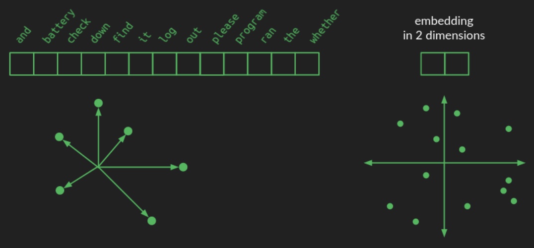
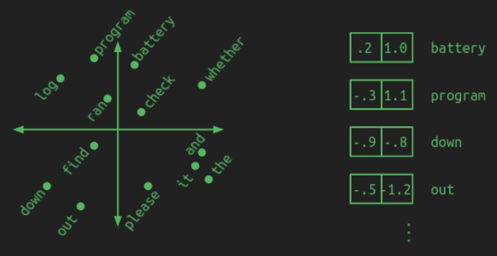
- By contrast, an embedding maps each word from this high-dimensional space into a lower-dimensional continuous space. In the language of linear algebra, this operation is known as projection. The image above illustrates how words might be projected into a two-dimensional space for illustrative purposes. Instead of needing \(N\) elements to represent each word, only two numbers—\((x, y)\) coordinates—are needed. A hypothetical 2D embedding for a small vocabulary is shown below, along with coordinates for some sample words:
-
A well-constructed embedding clusters semantically or functionally similar words near one another in this reduced space. Consequently, models trained in the embedding space learn generalized patterns that can be applied across groups of related words. For instance, if the model learns a transformation applicable to one word, that knowledge implicitly extends to all neighboring words in the embedded space. This property not only reduces the total number of parameters required but also significantly decreases the amount of training data needed to achieve generalization.
-
The illustration highlights how meaningful groupings may emerge: domain-specific nouns such as
battery,log, andprogrammay cluster in one region; prepositions likedownandoutin another; and verbs such ascheck,find, andranmay lie closer to the center. Although actual embeddings are generally more abstract and less visually interpretable, the core principle holds: semantic similarity corresponds to spatial proximity in the embedding space. -
Embeddings enable a drastic reduction in the number of trainable parameters. However, reducing dimensionality comes with a trade-off: semantic fidelity may be lost if too few dimensions are used. Rich linguistic structures and nuanced relationships require adequate space for distinct concepts to remain non-overlapping. Thus, the choice of embedding dimensionality reflects a compromise between computational efficiency and model expressiveness.
-
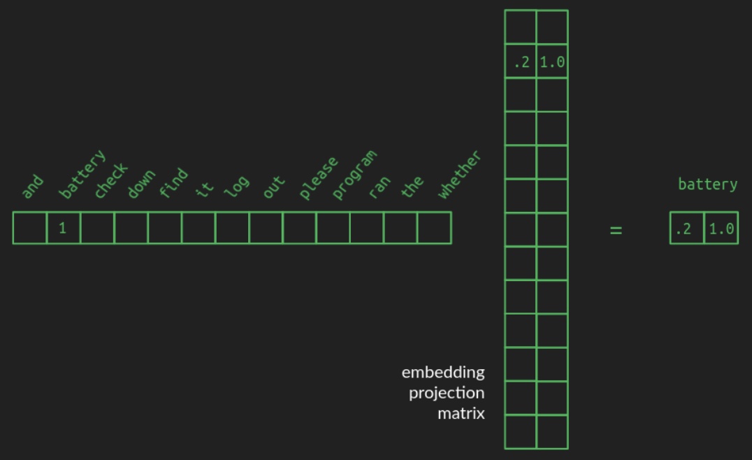
The transformation from a one-hot vector to its corresponding position in the embedded space is implemented as a matrix multiplication—a foundational operation in linear algebra and neural network design. Specifically, starting from a one-hot vector of shape \(1 \times N\), the word is projected into a space of dimension \(d\) (e.g., \(d = 2\)) using a projection matrix of shape \(N \times d\). The following diagram from Brandon Rohrer’s Transformers From Scratch illustrates such a projection matrix:
-
In the example, a one-hot vector representing the word
batteryselects the corresponding row in the projection matrix. This row contains the coordinates ofbatteryin the lower-dimensional space. For clarity, all other zeros in the one-hot vector and unrelated rows of the projection matrix are omitted in the diagram. In practice, however, the projection matrix is dense, with each row encoding a learned vector representation for its associated vocabulary word. -
Projection matrices can transform the original collection of one-hot vectors into arbitrary configurations in any target dimensionality. The core challenge lies in learning a useful projection—one that clusters related words and separates unrelated ones sufficiently. High-quality pre-trained embeddings (e.g., Word2Vec, GloVe) are available for many common languages. Nevertheless, in Transformer models, these embeddings are typically learned jointly during training, allowing them to adapt dynamically to the task at hand.
-
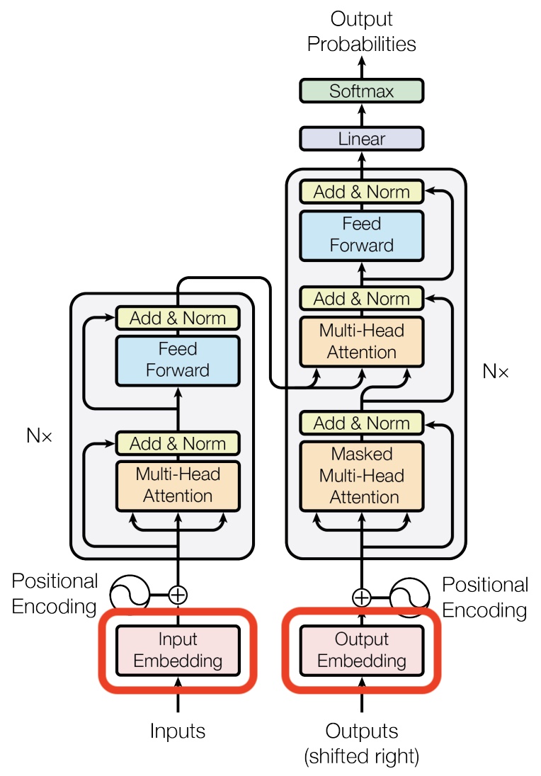
The placement of the embedding layer within the Transformer architecture is shown in the following diagram from the original Transformer paper:
Positional Encoding
In contrast to recurrent and convolutional neural networks, the Transformer architecture does not explicitly model relative or absolute position information in its structure.
- Up to this point, positional information for words has been largely overlooked, particularly for any words preceding the most recent one. Positional encodings (also known as positional embeddings) address this limitation by embedding spatial information into the transformer, allowing the model to comprehend the order of tokens in a sequence.
- Positional encodings are a crucial component of transformer models, enabling them to understand the order of tokens in a sequence. Absolute positional encodings, while straightforward, are limited in their ability to generalize to different sequence lengths. Relative positional encodings address some of these issues but at the cost of increased complexity. Rotary Positional Encodings offer a promising middle ground, capturing relative positions efficiently and enabling the processing of very long sequences in modern LLMs. Each method has its strengths and weaknesses, and the choice of which to use depends on the specific requirements of the task and the model architecture.
Absolute Positional Encoding
- Definition and Purpose:
- Absolute positional encoding, proposed in the original Transformer paper Attention Is All You Need (2017) by Vaswani et al., is a method used in transformer models to incorporate positional information into the input sequences. Since transformers lack an inherent sense of order, positional encodings are essential for providing this sequential information. The most common method, introduced in the original transformer model by Vaswani et al. (2017), is to add a circular wiggle to the embedded representation of words using sinusoidal positional encodings.
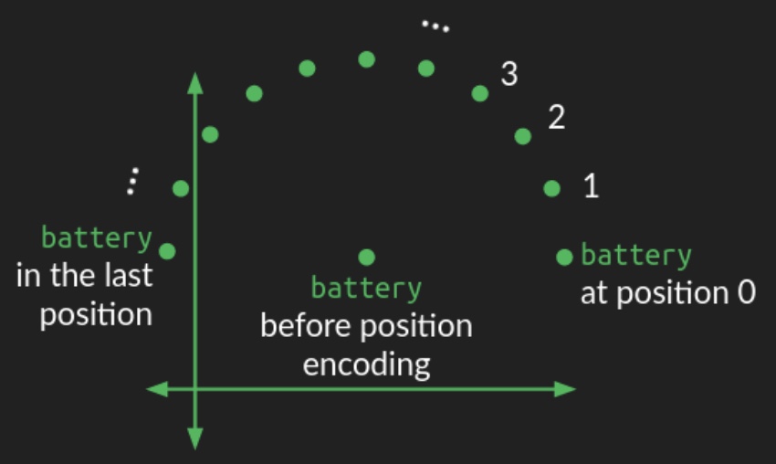
- The position of a word in the embedding space acts as the center of a circle. A perturbation is added based on the word’s position in the sequence, causing a circular pattern as you move through the sequence. Words that are close to each other in the sequence have similar perturbations, while words that are far apart are perturbed in different directions.
- Circular Wiggle:
- The following diagram from Brandon Rohrer’s Transformers From Scratch illustrates how positional encoding introduces this circular wiggle:
- Since a circle is a two-dimensional figure, representing this circular wiggle requires modifying two dimensions of the embedding space. In higher-dimensional spaces (as is typical), the circular wiggle is repeated across all other pairs of dimensions, each with different angular frequencies. In some dimensions, the wiggle completes many rotations, while in others, it may only complete a fraction of a rotation. This combination of circular wiggles of different frequencies provides a robust representation of the absolute position of a word within the sequence.
- Formula: For a position \(pos\) and embedding dimension \(i\), the embedding vector can be defined as:
\(PE_{(pos, 2i)} = \sin\left(\frac{pos}{10000^{2i/d_{model}}}\right)\)
\(PE_{(pos, 2i+1)} = \cos\left(\frac{pos}{10000^{2i/d_{model}}}\right)\)
- where \(d_{model}\) is the dimensionality of the model.
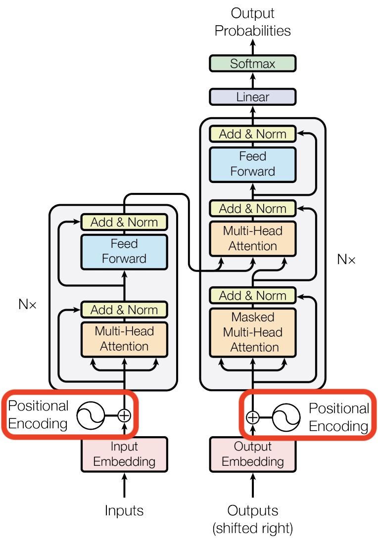
- Architecture Diagram: The architecture diagram from the original Transformer paper highlights how positional encoding is generated and added to the embedded words:
Why sinusoidal positional embeddings work?
- Absolute/sinusoidal positional embeddings add position information into the mix in a way that doesn’t disrupt the learned relationships between words and attention. For a deeper dive into the math and implications, Amirhossein Kazemnejad’s positional encoding tutorial is recommended.
Limitations of Absolute Positional Encoding
- Lack of Flexibility: While absolute positional encodings encode each position with a unique vector, they are limited in that they do not naturally generalize to unseen positions or sequences longer than those encountered during training. This poses a challenge when processing sequences of varying lengths or very long sequences, as the embeddings for out-of-range positions are not learned.
- Example: Consider a transformer trained on sentences with a maximum length of 100 tokens. If the model encounters a sentence with 150 tokens during inference, the positional encodings for positions 101 to 150 would not be well-represented, potentially degrading the model’s performance on longer sequences.
Relative Positional Encoding
- Definition and Purpose:
- Relative positional encoding, proposed in Self-Attention with Relative Position Representations (2018) by Shaw et al., addresses the limitations of absolute positional encoding by encoding the relative positions between tokens rather than their absolute positions. In this approach, the focus is on the distance between tokens, allowing the model to handle sequences of varying lengths more effectively.
- Relative positional encodings can be integrated into the attention mechanism of transformers. Instead of adding a positional encoding to each token, the model learns embeddings for the relative distances between tokens and incorporates these into the attention scores.
-
Relative Positional Encoding for a Sequence of Length N: For a sequence of length \(N\), the relative positions between any two tokens range from \(-N+1\) to \(N-1\). This is because the relative position between the first token and the last token in the sequence is \(-(N-1)\), and the relative position between the last token and the first token is \(N-1\). Therefore, we need \(2N-1\) unique relative positional encoding vectors to cover all possible relative distances between tokens.
- Example: If \(N = 5\), the possible relative positions range from \(-4\) (last token relative to the first) to \(+4\) (first token relative to the last). Thus, we need 9 relative positional encodings corresponding to the relative positions: \(-4, -3, -2, -1, 0, +1, +2, +3, +4\).
Limitations of Relative Positional Encoding
- Complexity and Scalability: While relative positional encodings offer more flexibility than absolute embeddings, they introduce additional complexity. The attention mechanism needs to account for relative positions, which can increase computational overhead, particularly for long sequences.
- Example: In scenarios where sequences are extremely long (e.g., hundreds or thousands of tokens), the number of relative positional encodings required (\(2N-1\)) can become very large, potentially leading to increased memory usage and computation time. This can make the model slower and more resource-intensive to train and infer.
Rotary Positional Embeddings (RoPE)
- Definition and Purpose:
- Rotary Positional Embeddings (RoPE), proposed in RoFormer: Enhanced Transformer with Rotary Position Embedding (2021) by Su et al., are a more recent advancement in positional encoding, designed to capture the benefits of both absolute and relative positional embeddings while being parameter-efficient. RoPE encodes absolute positional information using a rotation matrix, which naturally incorporates explicit relative position dependency in the self-attention formulation.
- RoPE applies a rotation matrix to the token embeddings based on their positions, enabling the model to infer relative positions directly from the embeddings. The very ability of RoPE to capture relative positions while being parameter-efficient has been key in the development of very long-context LLMs, like GPT-4, which can handle sequences of thousands of tokens.
- Mathematical Formulation: Given a token embedding \(x\) and its position \(pos\), the RoPE mechanism applies a rotation matrix \(R(pos)\) to the embedding:
-
The rotation matrix \(R(pos)\) is constructed using sinusoidal functions, ensuring that the rotation angle increases with the position index.
-
Capturing Relative Positions: The key advantage of RoPE is that the inner product of two embeddings rotated by their respective positions encodes their relative position. This means that the model can infer the relative distance between tokens from their embeddings, allowing it to effectively process long sequences.
-
Example: Imagine a sequence with tokens A, B, and C at positions 1, 2, and 3, respectively. RoPE would rotate the embeddings of A, B, and C based on their positions. The model can then determine the relative positions between these tokens by examining the inner products of their rotated embeddings. This ability to capture relative positions while maintaining parameter efficiency has been crucial in the development of very long-context LLMs like GPT-4, which can handle sequences of thousands of tokens.
-
Further Reading: For a deeper dive into the mathematical details of RoPE, Rotary Embeddings: A Relative Revolution by Eleuther AI offers a comprehensive explanation.
Limitations of Rotary Positional Embeddings
- Specificity of the Mechanism: While RoPE is powerful and efficient, it is specifically designed for certain architectures and may not generalize as well to all transformer variants or other types of models. Moreover, its mathematical complexity might make it harder to implement and optimize compared to more straightforward positional encoding methods.
- Example: In practice, RoPE might be less effective in transformer models that are designed with very different architectures or in tasks where positional information is not as crucial. For instance, in some vision transformers where spatial positional encoding is more complex, RoPE might not offer the same advantages as in text-based transformers.
Decoding Output Words / De-Embeddings / Un-Embeddings
-
While embedding words into a lower-dimensional continuous space significantly improves computational efficiency, at some point—particularly during inference or output generation—the model must convert these representations back into discrete tokens from the original vocabulary. This process, known as de-embedding (also commonly called un-embedding), occurs after the transformer has finished computing contextualized representations and is conceptually and operationally analogous to embedding: it involves a learned projection from one vector space to another, implemented via matrix multiplication.
-
In an autoregressive transformer, the specific vector that is de-embedded to predict the next token is the final hidden state at the last sequence position/index, i.e., the output representation corresponding to the last token generated so far. This hidden state is produced by passing the token’s initial embedding through a stack of transformer blocks (also known as transformer layers), where each block (layer) applies masked self-attention and feed-forward transformations that incorporate information from all preceding tokens—each of these operations are referred to as a sublayer when a transformer block is described as a layer. Concretely, at each attention layer, the last token’s current representation is linearly projected into its own query, key, and value (Q, K, V) vectors; its query is then compared against (i.e., attends over) the keys of all previous tokens to compute attention weights, which are used to form a weighted sum of the corresponding value vectors. The resulting attention output is combined with the token’s existing representation (via residual connections) and further transformed by a feed-forward network, yielding an updated representation for the last token that becomes its hidden state for the next layer.
-
Let \(H \in \mathbb{R}^{T \times d_{\text{model}}}\) denote the output of the final transformer layer. The hidden state corresponding to this last token, \(h_T\), is passed through a linear output projection (often called the output head or language modeling head) \(\text{logits} = h_T W_{\text{out}} + b_{\text{out}}\) followed by a softmax operation to produce a probability distribution over the vocabulary. Thus, the direct input to the de-embedding (un-embedding) step is \(h_T\) (and not the intermediate query, key, or value vectors).
How the De-Embedding Matrix Is Structured
-
The de-embedding matrix shares the same structural form as the embedding matrix, but with the number of rows and columns transposed. Specifically:
- The number of rows corresponds to the dimensionality of the embedding (or model) space—for example, 2 in the toy example used throughout this discussion.
- The number of columns equals the size of the vocabulary, which, in our running example, is 13.
-
This projection operation maps the lower-dimensional hidden representation back into the high-dimensional vocabulary space. The following diagram illustrates the structure of the de-embedding transformation:
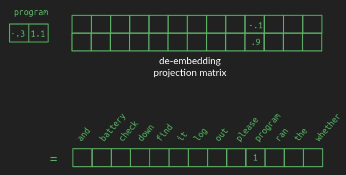
- Although the numerical values within a trained de-embedding (un-embedding) matrix are typically more difficult to visualize than those in an embedding matrix, the underlying mechanism is similar. When a contextualized hidden vector—specifically, the final hidden state of the last token, whose accumulated context strongly suggests the word
program—is multiplied by the de-embedding matrix, the resulting value at the output position corresponding toprogramwill be relatively high.
Relationship to Attention and Context Formation
-
It is important to clarify how this final hidden state is formed before de-embedding. Within each self-attention layer, the query vector of the last token is compared against the keys of all allowable previous tokens (due to causal masking), producing attention weights that determine how strongly the last token attends to each prior position. These weights are then used to form a weighted combination of the corresponding value vectors, yielding an attention output that represents context aggregated from earlier tokens.
-
This attention output is added back to the last token’s existing representation through a residual connection and passed through a position-wise feed-forward network, producing an updated hidden state for that token at the end of the layer. Repeating this process across layers progressively refines the last token’s hidden state, yielding (h_T), which summarizes all relevant prior context in the sequence. Once this representation is produced by the final layer, the intermediate Q, K, and V vectors have served their purpose and are not directly used during output prediction.
-
Due to the nature of projections from a lower-dimensional space into a higher-dimensional one, the output vector produced by de-embedding will not exhibit a sparse structure. Specifically:
- Nearby words in the embedding space—those with similar semantic or syntactic representations—will also receive moderate to high values.
- Dissimilar or unrelated words will generally yield values close to zero.
- Negative values may appear as well, depending on the structure of the de-embedding matrix and the input vector.
-
As a result, the output vector in the vocabulary space is dense. It contains mostly non-zero values and no longer resembles the one-hot vectors used for initial encoding. The following diagram illustrates such a representative dense result vector produced by de-embedding:
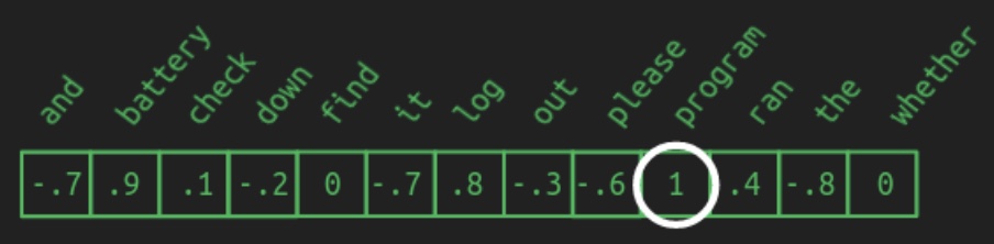
From Dense Scores to Discrete Tokens
-
To convert this dense output into a single discrete word, one common approach is to select the element with the highest value. This is referred to as the argmax operation, short for the “argument of the maximum.” The argmax returns the index (and thus the vocabulary word) associated with the maximum value in the output vector. This technique underlies greedy decoding, discussed previously in the section on sampling a sequence of output words, and serves as a strong baseline for sequence generation.
-
However, greedy decoding is not always optimal. If a contextualized hidden representation corresponds nearly equally well to multiple words, selecting only the highest-scoring one may sacrifice diversity and linguistic nuance. In such cases, always choosing the top prediction can result in repetitive or overly deterministic outputs.
-
Furthermore, more advanced sequence generation strategies—such as beam search or top-k sampling—require the model to evaluate multiple possible next tokens, sometimes several steps into the future, before committing to a final choice. To enable these strategies, the dense output vector produced from the de-embedding (un-embedding) of the last token’s final hidden state must first be transformed, via softmax, into a probability distribution over the vocabulary.
Attention
-
Having established the notions of linear projections (matrix multiplications) and vector spaces (dimensionalities), we can now revisit the attention mechanism in a more precise and formal manner. A careful accounting of matrix shapes at each stage helps clarify both the algorithm and its constraints. To that end, there is a small set of key quantities that recur throughout the discussion:
- \(N\): the vocabulary size; 13 in our running example, and typically on the order of tens of thousands in practical systems.
- \(n\): the maximum sequence length; 12 in our example. The original transformer paper leaves this implicit, but values on the order of a few hundred are common, while GPT-3 uses 2048.
- \(d_{model}\): the dimensionality of the embedding space used throughout the model (512 in the original paper).
-
The original input matrix is constructed by taking each word in the input sentence in its one-hot representation and stacking these vectors row-wise. Each row corresponds to a token position, and each column corresponds to a vocabulary item. The resulting input matrix therefore has \(n\) rows and \(N\) columns, which we denote as \([n \times N]\).
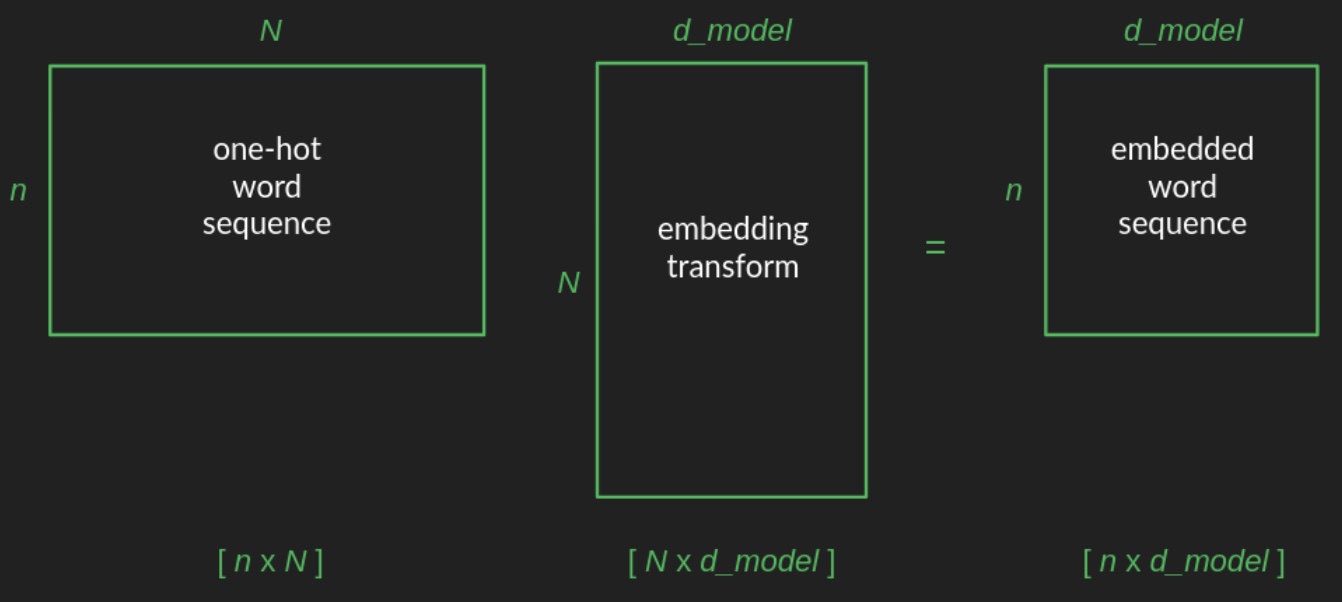
-
As discussed previously, the embedding matrix has \(N\) rows and \(d_{model}\) columns, giving it shape \([N \times d_{model}]\). By standard matrix multiplication rules, multiplying the input matrix \([n \times N]\) by the embedding matrix \([N \times d_{model}]\) produces an embedded sequence matrix of shape \([n \times d_{model}]\).
-
We can track the evolution of matrix shapes through the transformer as a way of maintaining intuition about the computation (see the figure below; source). After the embedding step, positional encodings are added elementwise rather than multiplied, so they do not alter the shape of the matrix. The resulting representation then passes through the attention layers and exits those layers with the same shape \([n \times d_{model}]\). Finally, the de-embedding (or un-embedding) projection maps this representation back into vocabulary space, yielding a score or probability for every word in the vocabulary at every position in the sequence.
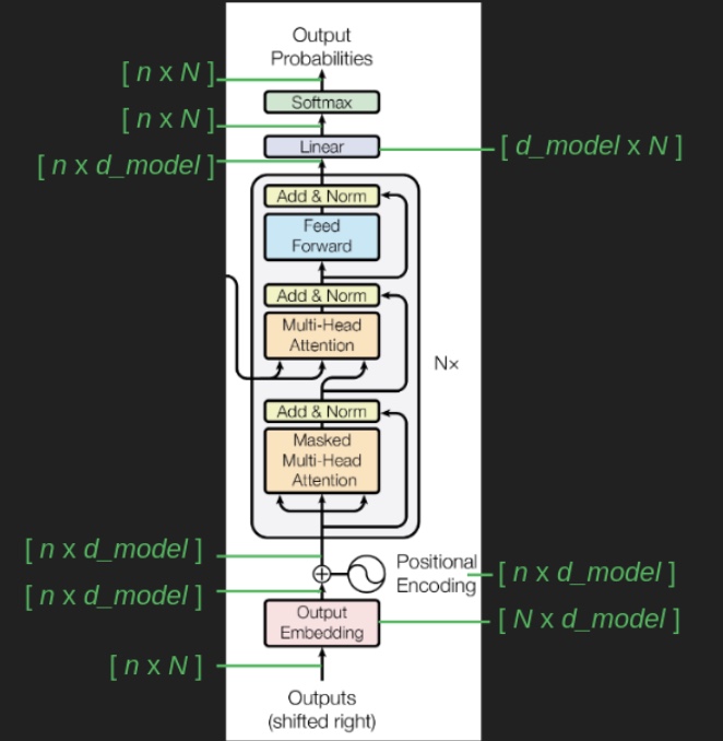
Dimensional Restrictions on Queries, Keys, and Values
-
Within each attention layer, the embedded representations are linearly projected into three distinct spaces corresponding to queries, keys, and values. These projections introduce three additional dimensionalities:
- \(d_q\): the dimensionality of the query vectors,
- \(d_k\): the dimensionality of the key vectors,
- \(d_v\): the dimensionality of the value vectors.
-
Starting from an input matrix of shape \([n \times d_{model}]\), the projection matrices have the following shapes:
\[W_Q \in \mathbb{R}^{d_{model} \times d_q}, \quad W_K \in \mathbb{R}^{d_{model} \times d_k}, \quad W_V \in \mathbb{R}^{d_{model} \times d_v},\]- … producing query, key, and value matrices of shapes \([n \times d_q]\), \([n \times d_k]\), and \([n \times d_v]\) respectively.
-
For the attention computation to be well-defined, the inner product between queries and keys must be computable. In particular, the compatibility score between a query and a key is given by a dot product, which requires the two vectors to live in the same space. This imposes the constraint \(d_q = d_k\). Without this equality, the matrix multiplication \(Q K^\top\) would be undefined, and the attention weights could not be computed.
-
The value dimension \(d_v\), by contrast, is not constrained by this compatibility requirement. Once attention weights are computed, they are used to form weighted sums of value vectors, and the resulting output simply inherits the dimensionality \(d_v\). In practice, many architectures choose \(d_q = d_k = d_v = \frac{d_{model}}{h}\) in the multi-head setting, where \(h\) is the number of attention heads, but this equality is a design choice rather than a mathematical necessity for \(d_v\).
-
Together, these dimensional relationships ensure that attention both preserves mathematical consistency and provides flexibility in how information is represented and transformed within the model.
Why attention? Contextualized Word Embeddings
History
- Bag of words was the first technique invented to create a machine-representation of text. By counting the frequency of words in a piece of text, one could extract its “characteristics”. The following table (source) shows an example of the data samples (reviews) per row and the vocabulary of the model (unique words) across columns.
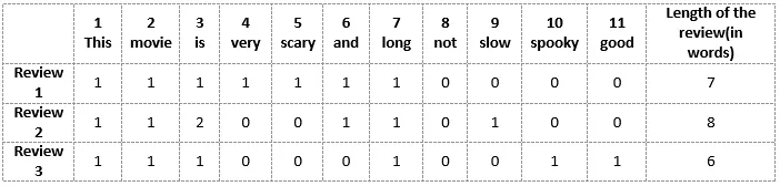
- However, this suggests that when all words are considered equally important, significant words like “crisis” which carry important meaning in the text can be drowned out by insignificant words like “and”, “for”, or “the” which add little information but are commonly used in all types of text.
- To address this issue, TF-IDF (Term Frequency-Inverse Document Frequency) assigns weights to each word based on its frequency across all documents. The more frequent the word is across all documents, the less weight it carries.
- However, this method is limited in that it treats each word independently and does not account for the fact that the meaning of a word is highly dependent on its context. As a result, it can be difficult to accurately capture the meaning of the text. This limitation was addressed with the use of deep learning techniques.
Enter Word2Vec: Neural Word Embeddings
- Word2Vec revolutionized embeddings by using a neural network to transform texts into vectors.
- Two popular approaches are the Continuous Bag of Words (CBOW) and Skip-gram models, which are trained using raw text data in an unsupervised manner. These models learn to predict the center word given context words or the context words given the center word, respectively. The resulting trained weights encode the meaning of each word relative to its context.
- The following figure (source) visualizes CBOW where the target word is predicted based on the context using a neural network:
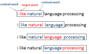
- However, Word2Vec and similar techniques (such as GloVe, FastText, etc.) have their own limitations. After training, each word is assigned a unique embedding. Thus, polysemous words (i.e, words with multiple distinct meanings in different contexts) cannot be accurately encoded using this method. As an example:
“The man was accused of robbing a bank.” “The man went fishing by the bank of the river.”
- As another example:
“Time flies like an arrow.” “Fruit flies like a banana.”
- This limitation gave rise to contextualized word embeddings.
Contextualized Word Embeddings
- Transformers, owing to their self-attention mechanism, are able to encode a word using its context. This, in turn, offers the ability to learn contextualized word embeddings.
- Note that while Transformer-based architectures (e.g., BERT) learn contextualized word embeddings, prior work (ELMo) originally proposed this concept.
- As indicated in the prior section, contextualized word embeddings help distinguish between multiple meanings of the same word, in case of polysemous words.
- The process begins by encoding each word as an embedding (i.e., a vector that represents the word and that LLMs can operate with). A basic one is one-hot encoding, but we typically use embeddings that encode meaning (the Transformer architecture begins with a randomly-initialized
nn.Embeddinginstance that is learnt during the course of training). However, note that the embeddings at this stage are non-contextual, i.e., they are fixed per word and do not incorporate context surrounding the word. - As we will see in the section on Single Head Attention Revisited, self-attention transforms the embedding to a weighted combination of the embeddings of all the other words in the text. This represents the contextualized embedding that packs in the context surrounding the word.
- Considering the example of the word bank above, the embedding for bank in the first sentence would have contributions (and would thus be influenced significantly) from words like “accused”, “robbing”, etc. while the one in the second sentence would utilize the embeddings for “fishing”, “river”, etc. In case of the word flies, the embedding for flies in the first sentence will have contributions from words like “go”, “soars”, “pass”, “fast”, etc. while the one in the second sentence would depend on contributions from “insect”, “bug”, etc.
- The following figure (source) shows an example for the word flies, and computing the new embeddings involves a linear combination of the representations of the other words, with the weight being proportional to the relationship (say, similarity) of other words compared to the current word. In other words, the output is computed as a weighted sum of the values, where the weight assigned to each value is computed by a compatibility function of the query with the corresponding key (also called the “alignment” function in Bengio’s original paper that introduced attention in the context of neural networks).
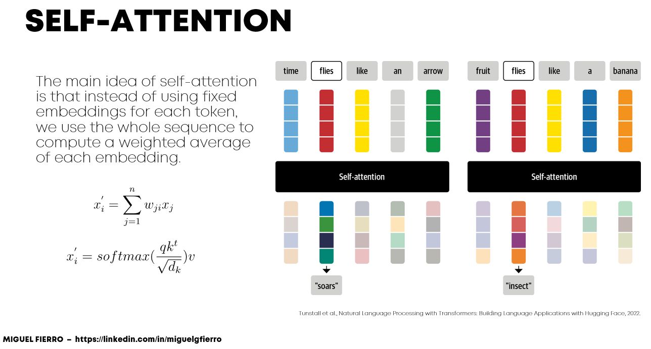
Types of Attention: Additive, Multiplicative (Dot-product), and Scaled
- The Transformer is based on “scaled dot-product attention”.
- The two most commonly used attention functions are additive attention (proposed by Bahdanau et al. (2015) in Neural Machine Translation by Jointly Learning to Align and Translate), and dot-product (multiplicative) attention. The scaled dot-product attention proposed in the Transformer paper is identical to dot-product attention, except for the scaling factor of \(\frac{1}{\sqrt{d_{k}}}\). Additive attention computes the compatibility function using a feed-forward network with a single hidden layer. While the two are similar in theoretical complexity, dot-product attention is much faster and more space-efficient in practice, since it can be implemented using highly optimized matrix multiplication code.
- While for small values of \(d_{k}\) the two mechanisms perform similarly, additive attention outperforms dot product attention without scaling for larger values of \(d_{k}\) (Massive Exploration of Neural Machine Translation Architectures). We suspect that for large values of \(d_{k}\), the dot products grow large in magnitude, pushing the softmax function into regions where it has extremely small gradients (To illustrate why the dot products get large, assume that the components of \(q\) and \(k\) are independent random variables with mean 0 and variance 1. Then their dot product, \(q \cdot k=\sum_{i=1}^{d_{k}} q_{i} k_{i}\), has mean 0 and variance \(d_{k}\).). To counteract this effect, we scale the dot products by \(\frac{1}{\sqrt{d_{k}}}\).
Attention calculation
- Let’s develop an intuition about the architecture using the language of mathematical symbols and vectors.
-
We update the hidden feature \(h\) of the \(i^{th}\) word in a sentence \(\mathcal{S}\) from layer \(\ell\) to layer \(\ell+1\) as follows:
\[h_{i}^{\ell+1}=\text { Attention }\left(Q^{\ell} h_{i}^{\ell}, K^{\ell} h_{j}^{\ell}, V^{\ell} h_{j}^{\ell}\right)\]-
i.e.,
\[\begin{array}{c} h_{i}^{\ell+1}=\sum_{j \in \mathcal{S}} w_{i j}\left(V^{\ell} h_{j}^{\ell}\right) \\ \text { where } w_{i j}=\operatorname{softmax}_{j}\left(Q^{\ell} h_{i}^{\ell} \cdot K^{\ell} h_{j}^{\ell}\right) \end{array}\]- where \(j \in \mathcal{S}\) denotes the set of words in the sentence and \(Q^{\ell}, K^{\ell}, V^{\ell}\) are learnable linear weights (denoting the Query, Key and \(V\)alue for the attention computation, respectively).
-
Pragmatic Intuition
- This section is aimed at understanding the underlying philosophy regarding how attention should be understood. The key point is to understand the rationale for employing three distinct vectors and to grasp the overarching objective of the entire attention mechanism.
-
Consider a scenario in which each token within a sequence must update its representation by incorporating relevant information from surrounding tokens, regardless of their proximity. Self-Attention provides a dynamic, learnable mechanism to facilitate this process. It begins by projecting each input token’s embedding into three distinct vectors:
- Query (\(Q\)): Represents the information the token seeks or is interested in. It can be thought of as the token formulating a question regarding the surrounding context.
- Key (\(K\)): Represents the information that the token offers or the types of queries it is capable of answering. It serves as a label or identifier of the token’s content.
- Value (\(V\)): Represents the actual content or substance of the token that will be conveyed if it is attended to. This constitutes the payload.
- The fundamental interaction occurs between the queries and the keys. For a given token’s query, the mechanism compares it against the keys of all tokens in the sequence through a scaled dot-product operation. This comparison produces a set of raw scores, indicating the relevance or compatibility between the query and each key. A higher score signifies that the key is highly pertinent to the query’s current information requirement.
- Subsequently, these raw scores are passed through a softmax function. This critical step normalizes the scores across all tokens, transforming them into a probability distribution that sums to one. These normalized scores serve as attention weights, determining the proportion of attention the query token allocates to each corresponding value token.
- Finally, a weighted sum of all Value vectors is computed, utilizing the attention weights obtained from the softmax operation. The outcome is an updated representation for the original Query token, blending information selectively from across the entire sequence based on learned relevance.
-
The true innovation of this mechanism lies in its adaptability. The attention weights are dynamically computed based on the specific input sequence and the learned Query, Key, and Value projection matrices. This enables the model to achieve:
- Token-Dependent Context: Different tokens can attend to various parts of the sequence depending on their unique role or informational needs.
- Input-Specific Routing: The attention patterns can vary significantly across different inputs, allowing flexible handling of syntax, semantics, and long-range dependencies.
- Focus: The model can learn to disregard irrelevant tokens by assigning them near-zero attention weights, thereby concentrating on the most important tokens.
Analogical Intuition
- From Eugene Yan’s Some Intuition on Attention and the Transformer blog, to build intuition around the concept of attention, let’s draw a parallel from a real life scenario and reason about the concept of key-value attention:
Imagine yourself in a library. You have a specific question (query). Books on the shelves have titles on their spines (keys) that suggest their content. You compare your question to these titles to decide how relevant each book is, and how much attention to give each book. Then, you get the information (value) from the relevant books to answer your question.
- We can understand the attention mechanism better through the following pipeline (source):
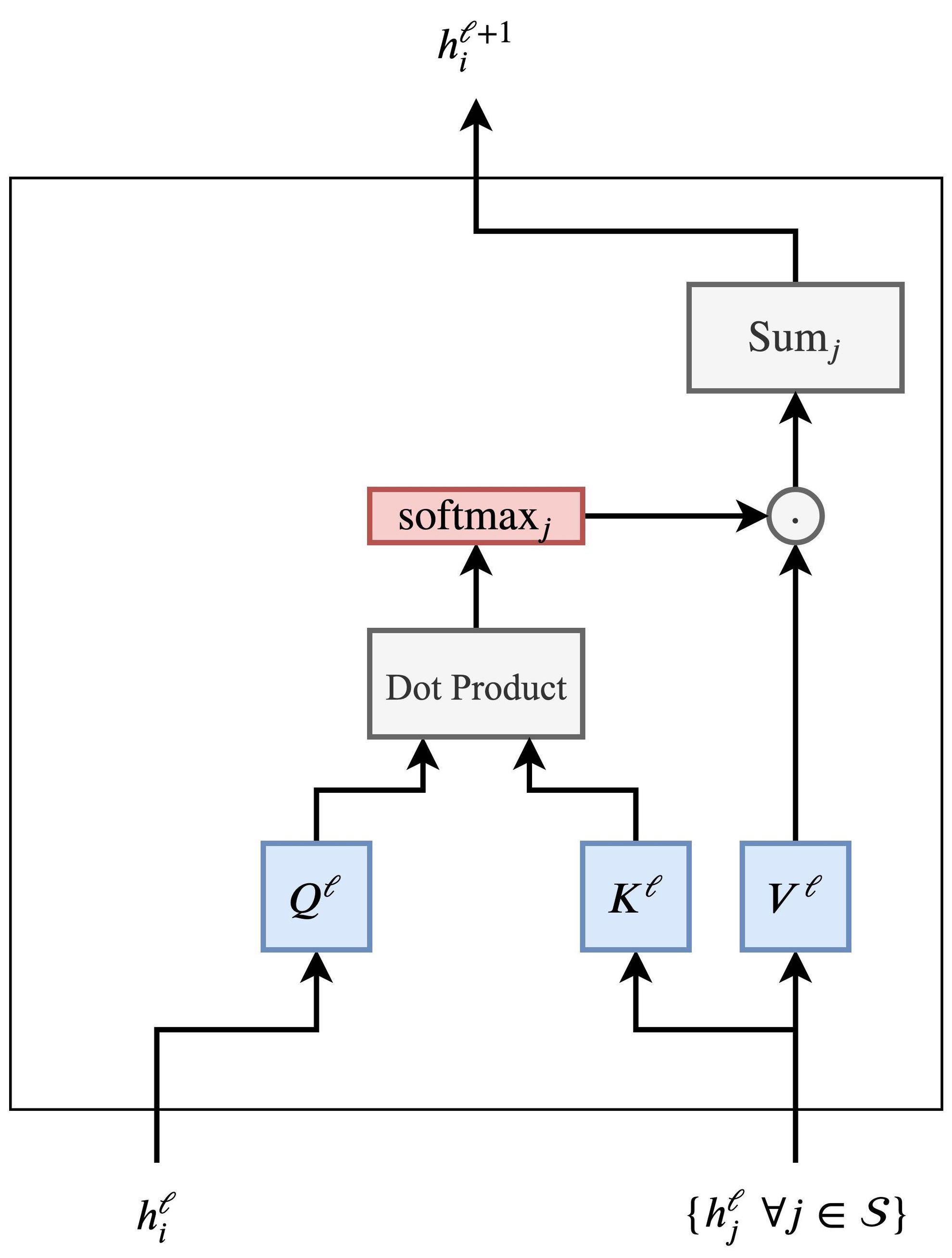
- Taking in the features of the word \(h_{i}^{\ell}\) and the set of other words in the sentence \({h_{j}^{\ell} \forall j \in \mathcal{S}}\), we compute the attention weights \(w_{i j}\) for each pair \((i, j)\) through the dot-product, followed by a softmax across all \(j\)’s.
- Finally, we produce the updated word feature \(h_{i}^{\ell+1}\) for word \(i\) by summing over all \({h_{j}^{\ell}}\)’s weighted by their corresponding \(w_{i j}\). Each word in the sentence undergoes the same pipeline in parallel to update its features.
- For more details on attention (including an overview of the various types and mathematical formulation of each), please refer the Attention primer.
Self-Attention
-
In self-attention, the input is modeled as three different components (or abstractions): the query, key, and value. These three components are derived from the same input sequence but are processed through different linear transformations to capture various relationships within the sequence.
- Query: Represents the element of the input sequence for which the attention score is being computed.
- Key: Represents the elements against which the query is compared to determine the attention score.
- Value: Represents the elements that are combined based on the attention scores to produce the output.
- Since the queries, keys, and values are all drawn from the same source, we refer to this as self-attention (we use “attention” and “self-attention” interchangeably in this primer). Self-attention forms the core component of Transformers. Also, given the use of the dot-product to ascertain similarity between the query and key vectors, the attention mechanism is also called dot-product self-attention.
- Note that one of the benefits of self-attention over recurrence is that it’s highly parallelizable. In other words, the attention mechanism is performed in parallel for each word in the sentence to obtain their updated features in one shot. This is a big advantage for Transformers over RNNs, which update features word-by-word. In other words, Transformer-based deep learning models don’t require sequential data to be processed in order, allowing for parallelization and reduced training time on GPUs compared to RNNs.
Single Head Attention Revisited
-
In the section on Attention as Matrix Multiplication, we explored a conceptual treatment of attention. While the actual implementation is more intricate, the earlier intuition remains foundationally useful. In practice, however, the queries and keys are no longer easily interpretable because they are projected into learned subspaces that are unique to each attention head.
-
In our conceptual model, each row in the queries matrix corresponded directly to a word in the vocabulary, represented via one-hot encoding—each vector uniquely identifying a word. In contrast, within a Transformer, each query is a vector in an embedded space, meaning that it no longer represents a single word in isolation but instead occupies a region near other words of similar semantic or syntactic roles.
-
Accordingly, the actual attention mechanism no longer establishes relationships between discrete, individual words. Rather, each attention head learns to map query vectors to points in a shared embedded space. This mapping enables attention to operate over clusters of semantically or contextually similar words, thus allowing for generalization across word types that play analogous roles. In essence, attention becomes a mechanism for establishing relationships between word groups, not just specific tokens.
Dimensional Flow Through Single-Head Attention
- Understanding the attention mechanism is greatly facilitated by tracking the matrix dimensions through the computation pipeline (adapted from source):
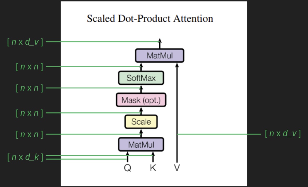
-
Let us consider the attention calculation step-by-step:
-
Let \(Q\) and \(K\) be the query and key matrices, respectively. Both have shape \([n \times d_k]\), where:
- \(n\) is the number of tokens (sequence length),
- \(d_k\) is the dimensionality of the key vectors for a single attention head.
-
More generally, the query vectors may be described with dimensionality \(d_q\), so that:
\[Q \in \mathbb{R}^{n \times d_q}, \quad K \in \mathbb{R}^{n \times d_k}\]- In standard Transformer architectures, these dimensions are chosen to be equal, yielding \(d_q = d_k\), which allows the dot-product attention computation to be well-defined and symmetric.
-
The attention scores are computed by the matrix multiplication \(QK^T\):
\[[n \times d_q] \cdot [d_k \times n] = [n \times n]\]- where the equality \(d_q = d_k\) ensures dimensional compatibility.
-
This results in a square matrix of attention scores, where each row corresponds to a query and each column to a key. The resulting \([n \times n]\) matrix expresses the relevance of each key to each query.
-
To ensure that the resulting values remain within a range conducive to stable training dynamics, each score is scaled by \(\frac{1}{\sqrt{d_k}}\). This mitigates the risk of excessively large dot products, which can cause the softmax function to saturate.
-
The softmax function is then applied to each row, converting scores into a probability distribution. This results in values that are non-negative, normalized across each row, and sharply peaked—often approximating an argmax operation.
-
The attention matrix, now shaped \([n \times n]\), effectively assigns contextual weights to each position in the sequence, specifying how much each token should attend to every other token.
-
These weights are then applied to the values matrix \(V\) (shaped \([n \times d_v]\)), producing a new representation of the input that emphasizes the most relevant parts of the sequence for each token.
-
The output of the attention mechanism is mathematically captured by the following equation:
\[\operatorname{Attention}(Q, K, V) = \underbrace{\operatorname{softmax} \left( \overbrace{\frac{QK^T}{\sqrt{d_k}}}^{\text{Attention Scores/Logits}} \right)}_{\text{Attention Weights}} V\]
-
-
At the end of each transformer block, this resulting representation is denoted by \(z\), which is the hidden state—i.e., the output representation produced by the transformer block for every token and passed to the next block or to the output head for language modeling.
Relationship Between \(d_{model}\) and Per-Head Dimensions
-
In a multi-head attention setting, the per-head dimensionalities of the query, key, and value vectors are directly tied to the model-wide embedding dimension \(d_{\text{model}}\). If the Transformer uses \(h\) attention heads, the standard design choice is:
\[d_q = d_k = d_v = \frac{d_{\text{model}}}{h}\]- This ensures that each attention head operates over a lower-dimensional subspace, and that concatenating the outputs of all heads recovers the original embedding size \(d_{\text{model}}\).
-
While the notation distinguishes \(d_q\) and \(d_k\) conceptually—reflecting their different functional roles in the attention computation—their equality in practice simplifies the architecture and preserves symmetry between queries and keys. Importantly, the scaling factor depends specifically on \(d_k\), since it governs the variance of the dot product \(QK^T\).
The attention function maps a query and a set of key-value pairs to an output, where the query, keys, values, and output are all vectors. The output is computed as a weighted sum of the values, with weights determined by a compatibility function (also known as an alignment function) between the query and the keys. This paradigm was originally introduced in Bahdanau et al. (2014), a foundational paper on attention in neural networks.
- A nontrivial aspect of this computation is that attention is calculated not just for the most recent word in the sequence, but simultaneously for every token in the input. This includes earlier words (whose output tokens have already been predicted) and future words (which have not yet been generated). While the attention scores for previous tokens are technically redundant at inference time, they are retained during training for completeness and symmetry. As for future tokens, although their predecessors have not yet been fixed, including them in the computation ensures consistent dimensions and allows indirect influence during training.
Attention Masking
-
Attention masking is a crucial refinement of the attention mechanism that constrains which positions in a sequence are allowed to interact. While the raw attention formulation computes pairwise relevance scores between all token positions, not all such interactions are valid in practice. Masking selectively removes invalid or undesirable position-to-position connections before the softmax is applied, ensuring that the resulting attention weights respect structural and semantic constraints of the task.
-
Masking operates by modifying the attention scores (i.e., attention logits) prior to normalization. Conceptually, disallowed positions are assigned a score of negative infinity. Because the softmax is defined as:
\[\text{softmax}(z_i) = \frac{e^{z_i}}{\sum_j e^{z_j}}\]- … setting \(z_i = -\infty\) ensures:
- … and therefore the corresponding attention probability is exactly zero. In practice, implementations replace literal negative infinity with a concrete value such as \(-10^9\) (or \(-\text{finfo.max}\) for the tensor’s data type), which is large enough that \(e^{-10^9} \approx 0\) under the softmax, while avoiding numerical issues during training.
-
Multiple masking constraints may apply simultaneously. When this occurs, masks are combined with logical OR semantics: a position is masked if any constraint deems it invalid. Numerically, this is implemented by adding mask matrices, where each entry is either \(0\) (allowed) or \(-\infty\) (masked). Addition reproduces OR behavior, since any sum involving \(-\infty\) remains \(-\infty\).
-
Causal masking and padding masking are types of attention masking. Causal masking enforces temporal ordering in autoregressive models by preventing a token at position \(i\) from attending to any position \(j > i\), while padding masking prevents attention to artificial padding tokens introduced for batch alignment. Both operate by modifying the attention logits prior to the softmax and therefore fall squarely under the general framework of attention masking.
-
As opposed to attention masking, loss masking does not modify the attention computation or the flow of information during the forward pass. Instead, it operates solely at the level of the training objective, zeroing out the loss for selected token positions such as padding tokens, prompt tokens in instruction tuning, or otherwise non-target tokens. These positions may still attend to and be attended by other tokens, but they contribute no gradient during backpropagation. In essence, attention masking restricts which token interactions are allowed, while loss masking restricts which model outputs are evaluated and optimized. A detailed overview of loss masking is available in the Loss Masking section.
Causal Masking
-
Causal masking (also known as look-ahead or triangular masking) enforces the temporal ordering required for sequential (i.e., auto-regressive) generation. When predicting the token at position \(i\), the model must not attend to tokens at positions \(j > i\), as these correspond to future information that has not yet been generated.
-
This mask is applied in the decoder self-attention layers only. The encoder processes the entire input sequence simultaneously and therefore does not require a causal constraint.
-
The causal mask is represented as an \([n \times n]\) matrix, where entries above the main diagonal are masked. Each row corresponds to a query position, and each column corresponds to a key position:
- The first row may attend only to the first token.
- The last row may attend to itself and all preceding tokens.
-
The mask is applied via element-wise addition to the scaled attention scores. Disallowed positions receive negative infinity, while allowed positions remain unchanged. The masked scores are then passed through the softmax, ensuring that future positions receive zero attention probability.
-
In The Annotated Transformer, this causal mask is visualized explicitly. The following figure depicts such a mask matrix for a sequence completion task:
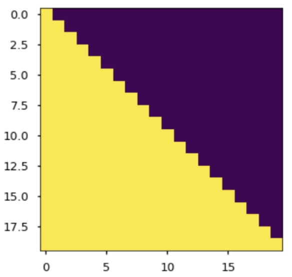
Padding Masking
-
Padding masking addresses a different concern: handling variable-length sequences within a batch. To enable efficient batching, shorter sequences are padded with special tokens that do not correspond to meaningful input. These padding positions must not contribute to, nor receive, attention.
-
Padding masks are applied wherever padding tokens may appear:
- in the encoder self-attention, to prevent real tokens from attending to padding,
- in the decoder self-attention, for the same reason,
- and in the encoder–decoder (cross) attention, to prevent decoder queries from attending to padded encoder positions.
-
Like causal masks, padding masks are implemented by assigning negative infinity to attention scores involving padded positions. After softmax, these positions receive zero probability and are effectively ignored.
-
In the decoder self-attention, padding and causal masks are combined. A position is masked if it is either a future position or a padding token. This combined mask is added to the attention scores:
\[\text{softmax}\left(\frac{QK^T}{\sqrt{d_k}} + M_{\text{causal}} + M_{\text{pad}}\right)\]- … ensuring that both temporal constraints and padding constraints are simultaneously enforced.
-
Note that the summing mask matrices whose entries are either \(0\) for allowed positions or \(-\infty\) for masked ones emulates logical OR semantics. Because any sum that includes \(-\infty\) remains \(-\infty\), a position is masked whenever at least one masking constraint deems it invalid.
-
A final conceptual shift is worth emphasizing: attention masks operate over positions, not over word identities. The \([n \times n]\) attention matrix specifies which positions may interact, independent of the underlying vocabulary. Masking simply removes invalid position-to-position links, while the softmax renormalizes the remaining interactions into a coherent probability distribution that respects both sequence structure and batching requirements.
Why is the product of the \(Q\) and \(K\) matrix in Self-Attention normalized?
- Let’s break down the reasoning behind normalizing the dot product of \(Q\) and \(K\) by the square root of the dimension of the keys.
Understanding the Role of \(Q\) and \(K\) in Self-Attention
-
In self-attention, each input token is associated with three vectors: the Query (\(Q\)), the Key (\(K\)), and the Value (\(V\)):
- Query (\(Q\)): Represents the current token for which we are computing the attention score. It is essentially asking, “To which other tokens should I pay attention?”
- Key (\(K\)): Represents each of the tokens that can be attended to. It acts as the potential target of attention, answering the question, “How relevant am I to a given query?”
- Value (\(V\)): Contains the actual information or feature vectors to be aggregated based on the attention scores.
Dot Product of \(Q\) and \(K\)
- To compute the attention score between a query and a key, we perform a dot product between the query vector \(q_i\) and each key vector \(k_j\):
- The result of this dot product gives us a measure of similarity or relevance between the current token (represented by the query) and another token (represented by the key). High dot product values indicate a high degree of similarity or relevance, suggesting that the model should pay more attention to this token.
Need for Normalization
-
Without normalization, the dot product values can become very large, especially when the dimensionality of the query and key vectors (\(d_k\)) is high. This is due to the following reasons:
- Magnitude Dependency: The dot product value is dependent on the dimensionality of the vectors. As the dimensionality increases, the magnitude of the dot product can also increase significantly, leading to a wider range of possible values.
- Gradient Instability: Large values in the dot product can cause the softmax function, which is used to convert attention scores into probabilities, to saturate. When the input values to softmax are large, it can result in a gradient that is too small, slowing down the learning process or causing vanishing gradient problems.
- Training Stability: Large variance in the attention scores can cause instability during training. If the scores are too large, the model’s output can become overly sensitive to small changes in input, making it difficult to learn effectively.
Normalization by Square Root of \(d_k\)
- To mitigate these issues, the dot product is scaled by the square root of the dimensionality of the key vectors (\(\sqrt{d_k}\)):
-
Here’s why this specific form of normalization is effective:
-
Variance Control: By scaling the dot product by \(\sqrt{d_k}\), we ensure that the variance of the dot product remains approximately constant and doesn’t grow with the dimensionality. This keeps the distribution of attention scores stable, preventing any single score from dominating due to large values.
-
Balanced Softmax Output: The scaling keeps the range of attention scores in a region where the softmax function can operate effectively. It prevents the softmax from becoming too peaked or too flat, ensuring that attention is distributed appropriately among different tokens.
-
Intuitive Interpretation
- The normalization can be interpreted as adjusting the scale of the dot product to make it invariant to the dimensionality of the vectors. Without this adjustment, as the dimensionality of the vectors increases, the dot product’s expected value would increase, making it harder to interpret the similarity between query and key. Scaling by \(\sqrt{d_k}\) effectively counteracts this growth, maintaining a stable range of similarity measures.
Takeaways
-
In summary, the normalization of the product of the \(Q\) and \(K\) matrices in self-attention is essential for:
- Controlling the variance of the attention scores.
- Ensuring stable and efficient training.
- Keeping the attention distribution interpretable and effective.
-
This scaling step is a simple yet crucial modification that significantly improves the performance and stability of self-attention mechanism in models like Transformers.
Putting it all together
- The following infographic (source) provides a quick overview of the constituent steps to calculate attention.
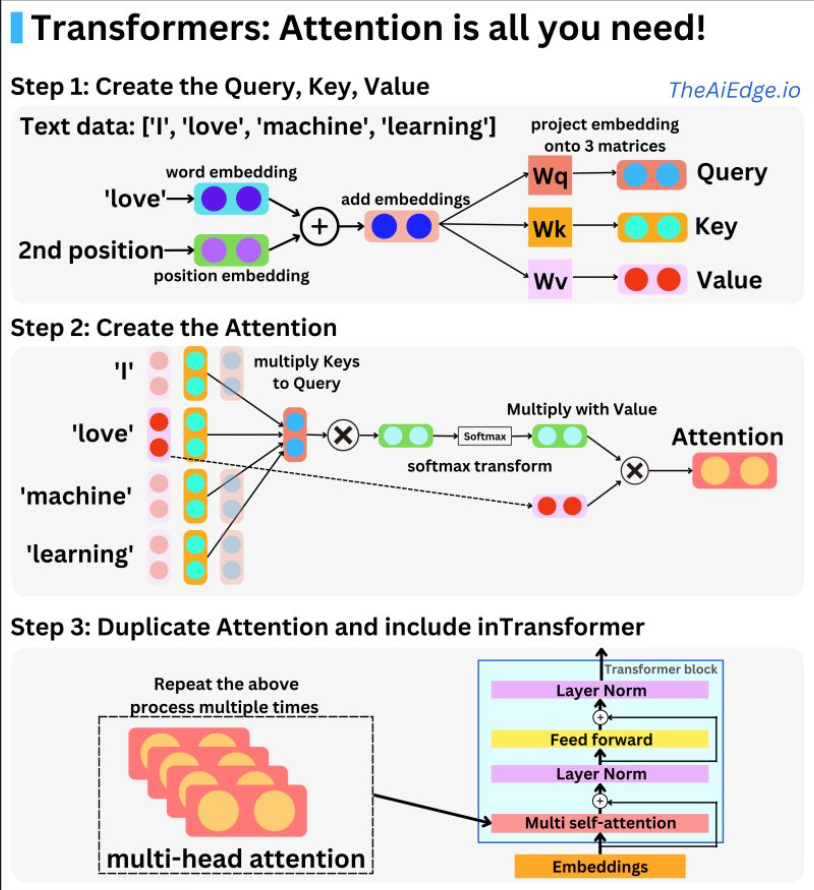
- As indicated in the section on Contextualized Word Embeddings, Attention enables contextualized word embeddings by allowing the model to selectively focus on different parts of the input sequence when making predictions. Put simply, the attention mechanism allows the transformer to dynamically weigh the importance of different parts of the input sequence based on the current task and context.
- In an attention-based model like the transformer, the word embeddings are combined with attention weights that are learned during training. These weights indicate how much attention should be given to each word in the input sequence when making predictions. By dynamically adjusting the attention weights, the model can focus on different parts of the input sequence and better capture the context in which a word appears. As the paper states, the attention mechanism is what has revolutionized Transformers to what we see them to be today.
- Upon encoding a word as an embedding vector, we can also encode the position of that word in the input sentence as a vector (positional embeddings), and add it to the word embedding. This way, the same word at a different position in a sentence is encoded differently.
- The attention mechanism works with the inclusion of three vectors: key, query, value. Attention is the mapping between a query and a set of key-value pairs to an output. We start off by taking a dot product of query and key vectors to understand how similar they are. Next, the Softmax function is used to normalize the similarities of the resulting query-key vectors. The output is computed as a weighted sum of the values, where the weight assigned to each value is computed by a compatibility function of the query with the corresponding key.
- Thus, the basis behind the concept of attention is: “How much attention a word should pay to another word in the input to understand the meaning of the sentence?”
- As indicated in the section on Attention Calculation, one of the benefits of self-attention over recurrence is that it’s highly parallelizable. In other words, the attention mechanism is performed in parallel for each word in the sentence to obtain their updated features in one shot. Furthermore, learning long-term/long-range dependencies in sequences is another benefit.
- The architecture diagram from the original Transformer paper highlights the self-attention layer (in multi-head form in both the encoder (unmasked variant) and decoder (masked variant):
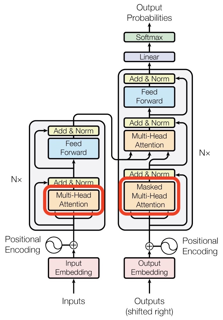
Coding up self-attention
Single Input
- To ensure that the matrix multiplications in the scaled dot-product attention function are valid, we need to add assertions to check the shapes of \(Q\), \(K\), and \(V\). Specifically, after transposing \(K\), the last dimension of \(Q\) should match the first dimension of \(K^T\) for the multiplication \(QK^T\) to be valid. Similarly, for the multiplication of the attention weights and \(V\), the last dimension of the attention weights should match the first dimension of \(V\).
- Here’s the updated code with these assertions:
import numpy as np
from scipy.special import softmax

def scaled_dot_product_attention_single(Q: np.ndarray, K: np.ndarray, V: np.ndarray) -> np.ndarray:
    """
    Implements scaled dot-product attention for a single input using NumPy.
    Includes shape assertions for valid matrix multiplications.

    Parameters:
    Q (np.ndarray): Query array of shape [seq_len, d_q].
    K (np.ndarray): Key array of shape [seq_len, d_k].
    V (np.ndarray): Value array of shape [seq_len, d_v].

    Returns:
    np.ndarray: Output array of the attention mechanism.
    """

    # Ensure the last dimension of Q matches the first dimension of K^T (or equivalently, the last dimension of K)
    # In other words, we're checking if d_q == d_k
    assert Q.shape[-1] == K.shape[-1], "The last dimension of Q must match the first dimension of K^T (d_q == d_k)"

    # Ensure the last dimension of attention weights (i.e., last dimension of K^T or equivalently, the first dimension of K) matches the first dimension of V
    # In other words, we're checking if the sequence lengths match between K and V
    assert K.shape[0] == V.shape[0], "The first dimension of K must match the first dimension of V (sequence length)"

    d_k = Q.shape[-1]  # Dimension of the key vectors

    # Calculate dot products of Q with K^T and scale
    scores = np.matmul(Q, K^T) / np.sqrt(d_k)

    # Apply softmax to get attention weights
    attn_weights = softmax(scores, axis=-1)

    # Multiply by V to get output
    output = np.matmul(attn_weights, V)

    return output

# Test with sample input
def test_with_sample_input():
    # Sample inputs
    Q = np.array([[1, 0], [0, 1]])
    K = np.array([[1, 0], [0, 1]])
    V = np.array([[1, 2], [3, 4]])

    # Function output
    output = scaled_dot_product_attention_single(Q, K, V)

    # Manually calculate expected output
    d_k = Q.shape[-1]
    scores = np.matmul(Q, K^T) / np.sqrt(d_k)
    attn_weights = softmax(scores, axis=-1)
    expected_output = np.matmul(attn_weights, V)
- Explanation:
- Two assertions are added:
- \(Q\) and \(K^T\) Multiplication: Checks that the last dimension of \(Q\) matches the first dimension of \(K^T\) (or equivalently, the last dimension of \(K\)).
- Attention Weights and \(V\) Multiplication: Ensures that the last dimension of \(K^T\) (or equivalently, the first dimension of \(K\)) matches the first dimension of \(V\), as the shape of the attention weights will align with the shape of \(K^T\) after softmax.
- Note that these shape checks are critical for the correctness of matrix multiplications involved in the attention mechanism. By adding these assertions, we ensure the function handles inputs with appropriate dimensions, avoiding runtime errors due to invalid matrix multiplications.
- Two assertions are added:
Batch Input
- In the batched version, the inputs \(Q\), \(K\), and \(V\) will have shapes
[batch_size, seq_len, feature_size]. The function then needs to perform operations on each item in the batch independently.
import numpy as np
from scipy.special import softmax

def scaled_dot_product_attention_batch(Q: np.ndarray, K: np.ndarray, V: np.ndarray) -> np.ndarray:
    """
    Implements scaled dot-product attention for batch input using NumPy.
    Includes shape assertions for valid matrix multiplications.

    Parameters:
    Q (np.ndarray): Query array of shape [batch_size, seq_len, d_q].
    K (np.ndarray): Key array of shape [batch_size, seq_len, d_k].
    V (np.ndarray): Value array of shape [batch_size, seq_len, d_v].

    Returns:
    np.ndarray: Output array of the attention mechanism.
    """

    # Ensure batch dimensions of Q, K, V match
    assert Q.shape[0] == K.shape[0] == V.shape[0], "Batch dimensions of Q, K, V must match"

    # Ensure the last dimension of Q matches the first dimension of K^T (or equivalently, the last dimension of K)
    # In other words, we're checking if d_q == d_k
    assert Q.shape[-1] == K.shape[-1], "The last dimension of Q must match the last dimension of K"

    # Ensure the last dimension of attention weights (i.e., last dimension of K^T or equivalently, the second dimension of K) matches the second dimension of V
    # In other words, we're checking if the sequence lengths match between K and V
    assert K.shape[1] == V.shape[1], "The first dimension of K must match the first dimension of V"

    d_k = Q.shape[-1]

    # Calculate dot products of Q with K^T for each batch and scale
    scores = np.matmul(Q, K.transpose(0, 2, 1)) / np.sqrt(d_k)

    # Apply softmax to get attention weights for each batch
    attn_weights = softmax(scores, axis=-1)

    # Multiply by V to get output for each batch
    output = np.matmul(attn_weights, V)

    return output

# Example test case for batched input
def test_with_batch_input():
    batch_size, seq_len, feature_size = 2, 3, 4
    Q_batch = np.random.randn(batch_size, seq_len, feature_size)
    K_batch = np.random.randn(batch_size, seq_len, feature_size)
    V_batch = np.random.randn(batch_size, seq_len, feature_size)

    output = scaled_dot_product_attention_batch(Q_batch, K_batch, V_batch)

    assert output.shape == (batch_size, seq_len, feature_size), "Output shape is incorrect for batched input"
- Explanation:
- The function now expects inputs with an additional batch dimension at the beginning.
- The shape assertions are updated to ensure that the batch dimensions of \(Q\), \(K\), and \(V\) match, and the feature dimensions are compatible for matrix multiplication.
- Matrix multiplications (
np.matmul) and the softmax operation are performed independently for each item in the batch. - The test case
test_with_batch_inputdemonstrates how to use the function with batched input and checks if the output shape is correct.
Averaging is equivalent to uniform attention
- On a side note, it is worthwhile noting that the averaging operation is equivalent to uniform attention with the weights being all equal to \(\frac{1}{n}\), where \(n\) is the number of words in the input sequence. In other words, averaging is simply a special case of attention.
Activation Functions
- The transformer does not use an activation function following the multi-head attention layer, but does use the ReLU activation sandwiched between the two position-wise fully-connected layers that form the feed-forward network. Put simply, the a fully connected feed-forward network in the transformer blocks consists of two linear transformations with a ReLU activation in between.
- The reason behind this goes back to the purpose of self-attention. The measure between word-vectors is generally computed through cosine-similarity because in the dimensions word tokens exist, it’s highly unlikely for two words to be collinear even if they are trained to be closer in value if they are similar. However, two trained tokens will have higher cosine-similarity if they are semantically closer to each other than two completely unrelated words.
- This fact is exploited by the self-attention mechanism; after several of these matrix multiplications, the dissimilar words will zero out or become negative due to the dot product between them, and the similar words will stand out in the resulting matrix.
- Thus, self-attention can be viewed as a weighted average, where less similar words become averaged out faster (toward the zero vector, on average), thereby achieving groupings of important and unimportant words (i.e., attention). The weighting happens through the dot product. If input vectors were normalized, the weights would be exactly the cosine similarities.
- The important thing to take into consideration is that within the self-attention mechanism, there are no inherent parameters; those linear operations are just there to capture the relationship between the different vectors by using the properties of the vectors used to represent them, leading to attention weights.
Attention in Transformers: What is new and what is not?
-
The Transformer model introduced by Vaswani et al. (2017) adopts the sequence-to-sequence encoder–decoder paradigm that predates Transformers by several years. This architectural framework was popularized in neural machine translation by works such as Neural Machine Translation by Jointly Learning to Align and Translate by Bahdanau et al. (2014), from Yoshua Bengio’s research group. In this paradigm, an encoder maps an input sequence into a continuous representation, and a decoder generates the output sequence conditioned on this representation. The Transformer therefore does not introduce the encoder–decoder formulation itself, but rather instantiates it using a different set of computational primitives than recurrent or convolutional models.
-
Transformers employ scaled dot-product attention, parameterized by Query, Key, and Value matrices, as described in Attention Is All You Need by Vaswani et al. (2017). This formulation is closely related to similarity-based retrieval mechanisms long studied in information retrieval and memory-augmented models, where relevance is computed via dot products or cosine similarity between query and key representations. Earlier neural machine translation models, including the work by Bahdanau et al. (2014), relied on additive attention, often referred to as Bahdanau attention, which computes alignment scores using a learned feedforward network. While effective, this earlier form of attention is computationally more expensive and less amenable to parallelization than dot-product-based variants. Subsequent work such as Effective Approaches to Attention-based Neural Machine Translation by Luong et al. (2015) further explored multiplicative attention, narrowing the conceptual gap between earlier attention mechanisms and the scaled dot-product attention later used in Transformers.
-
The primary conceptual innovation of the Transformer lies in its systematic use of attention within the encoder itself. Earlier sequence-to-sequence models with attention applied it exclusively as cross-attention in the decoder, allowing the decoder to attend over a sequence of encoder states produced without internal attention, as in Neural Machine Translation by Jointly Learning to Align and Translate by Bahdanau et al. (2014) and Learning Phrase Representations using RNN Encoder–Decoder for Statistical Machine Translation by Cho et al. (2014). In contrast, Transformers replace recurrence entirely by applying attention to relate all positions within the same sequence, both in the encoder and in the decoder, whereas prior sequence-to-sequence architectures with attention restricted its use to the decoder side as cross-attention over encoder states and did not apply attention mechanisms within the encoder itself. This mechanism, now commonly referred to as self-attention, enables each token to directly attend to every other token in the sequence, facilitating the modeling of long-range dependencies while allowing full parallelization during training. Subsequent analyses and extensions, such as On the Properties of Attention Networks by Jain and Wallace (2019) and A Survey on Transformers by Lin et al. (2021), further clarify that while attention itself was not new, its exclusive and pervasive use as the core computational operation is what fundamentally distinguishes Transformers from earlier neural architectures.
Calculating \(Q\), \(K\), and \(V\) matrices in the Transformer architecture
- Each word is embedded into a vector of size 512 and is fed into the bottom-most encoder. The abstraction that is common to all the encoders is that they receive a list of vectors each of the size 512 – in the bottom encoder that would be the word embeddings, but in other encoders, it would be the output of the encoder that is directly below. The size of this list is hyperparameter we can set – basically it would be the length of the longest sentence in our training dataset.
- In the self-attention layers, multiplying the input vector (which is the word embedding for the first block of the encoder/decoder stack, while the output of the previous block for subsequent blocks) by the attention weights matrix (which are the \(Q\), \(K\), and \(V\) matrices stacked horizontally) and adding a bias vector afterwards results in a concatenated key, value, and query vector for this token. This long vector is split to form the \(q\), \(k\), and \(v\) vectors for this token (which actually represent the concatenated output for multiple attention heads and is thus, further reshaped into \(q\), \(k\), and \(v\) outputs for each attention head — more on this in the section on Multi-head Attention). From Jay Alammar’s: The Illustrated GPT-2:
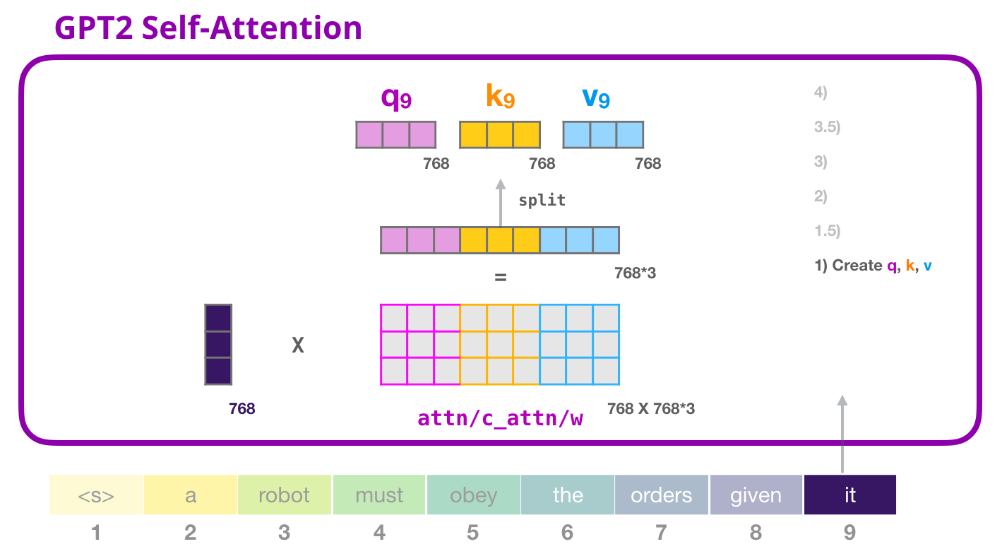
Calculating \(Q\), \(K\), and \(V\) matrices in the Transformer architecture
-
In the original Transformer architectures, each input token is mapped to a fixed-dimensional vector using a learned embedding table, with the model dimension \(d_{\text{model}} = 512\) for the Transformer base configuration and \(d_{\text{model}} = 1024\) for the Transformer big configuration, as introduced in Attention Is All You Need by Vaswani et al. (2017). These embedding vectors are provided as input to the first encoder layer. More generally, every encoder layer in the stack consumes a sequence of vectors of identical dimensionality $d_{\text{model}}$. For the first layer, these vectors correspond to token embeddings combined with positional encodings, while for later layers they correspond to the output activations (i.e., feature maps) of the immediately preceding encoder layer. The length of this sequence equals the model’s sequence length, which is determined by the input sentence length and typically padded or truncated to a predefined maximum sequence length that acts as a hyperparameter during training and inference.
-
Within each self-attention sublayer, every input vector \(x \in \mathbb{R}^{d_{\text{model}}}\) is independently transformed into a query, key, and value representation through learned linear projections. Concretely, the model learns three parameter matrices \(W_Q\), \(W_K\), and \(W_V\), each of shape \(d_{\text{model}} \times d_{\text{model}}\), along with corresponding bias terms. In practice, many implementations compute these projections efficiently by applying a single linear transformation whose weight matrix is the horizontal concatenation of \(W_Q\), \(W_K\), and \(W_V\), followed by a bias addition. The resulting vector is then split into the query (\(q\)), key (\(k\)), and value (\(v\)) components for that token. These \(q\), \(k\), and \(v\) vectors typically represent concatenated outputs for all attention heads. They are therefore reshaped into per-head representations of dimensionality \(d_k = d_v = d_{\text{model}} / h\), where \(h\) denotes the number of attention heads, as detailed in the multi-head attention mechanism (cf. the section on Multi-head Attention for a detailed discourse).
-
A clear visual illustration of this projection and splitting process is provided in The Illustrated GPT-2 by Jay Alammar, which builds on the Transformer formulation and its application to autoregressive language models such as GPT-2 (Language Models are Unsupervised Multitask Learners by Radford et al. (2019)). The following figure, adapted from Jay Alammar’s: The Illustrated GPT-2, shows how, for a given input token in GPT-2, the model first constructs concatenated query, key, and value vectors via learned linear projections, and then splits and reshapes these vectors into multiple attention heads, each operating on lower-dimensional \(Q\), \(K\), and \(V\) representations that jointly enable multi-head self-attention over the input sequence.
Optimizing Performance with the KV Cache
- Using a KV cache is one of the most commonly used tricks for speeding up inference with Transformer-based models, particularly employed with LLMs. Let’s unveil its inner workings.
- Autoregressive decoding process: When we perform inference with an LLM, it follows an autoregressive decoding process. Put simply, this means that we (i) start with a sequence of textual tokens, (ii) predict the next token, (iii) add this token to our input, and (iv) repeat until generation is finished.
- Causal self-attention: Self-attention within a language model is causal, meaning that each token only considers itself and prior tokens when computing its representation (i.e., not future tokens). As such, representations for each token do not change during autoregressive decoding! We need to compute the representation for each new token, but other tokens remain fixed (i.e., because they don’t depend on tokens that follow them).
- Caching self-attention values: When we perform self-attention, we project our sequence of tokens using three separate, linear projections: key projection, value projection, and query projection. Then, we execute self-attention using the resulting matrices. The KV-cache simply stores the results of the key and value projections for future decoding iterations so that we don’t recompute them every time!
- Why not cache the query? So why are the key and value projections cached, but not the query? This is simply because the entries in the query matrix are only needed to compute the representations of prior tokens in the sequence (whose key and value representations are already stored in the KV-Cache). At each time-step, the new query input consists of the token at that time-step and all prior tokens (i.e., the entire sequence up to that point). For computing the representation of query representation for the most recent token, we only need access to the most recent row in the query matrix.
- Updates to the KV cache: Throughout autoregressive decoding, we have the key and value projections cached. Each time we get a new token in our input, we simply compute the new rows as part of self-attention and add them to the KV cache. Then, we can use the query projection for the new token and the updated key and value projections to perform the rest of the forward pass.
- Latency optimization: KV-caching decreases the latency to the next token in an autoregressive setting starting from the second token. Since the prompt tokens are not cached at the beginning of the generation, time to the first token is high, but as KV-caching kicks in for further generation, latency reduces. In other words, KV-caching is the reason why the latency of the first token’s generation (from the time the input prompt is fed in) is higher than that of consecutive tokens.
- Scaling to Multi-head Self-attention: Here, we have considered single-head self-attention for simplicity. However, it’s important to note that the same exact process applies to the multi-head self-attention used by LLMs (detailed in the Multi-Head Attention section below). We just perform the exact same process in parallel across multiple attention heads.
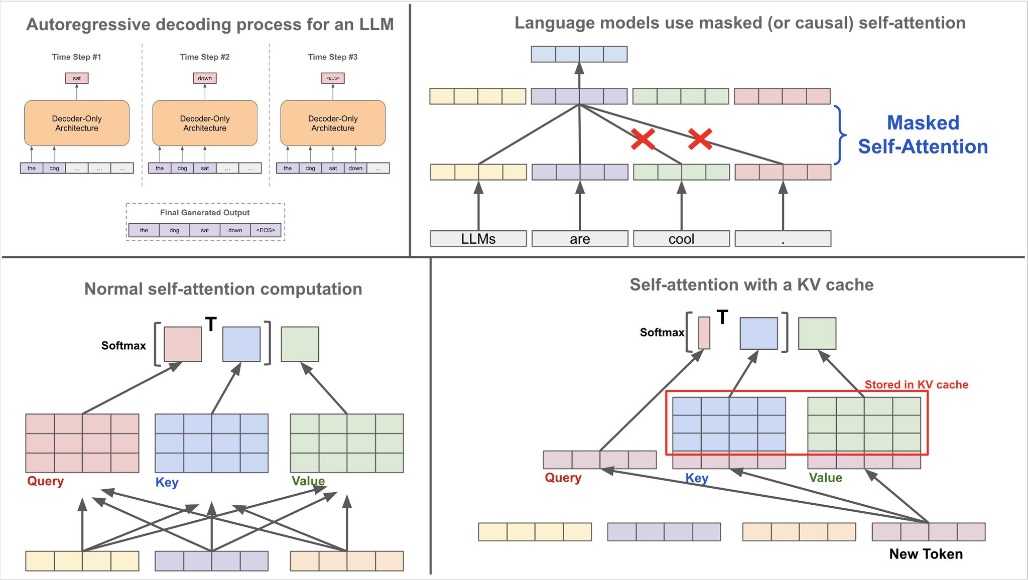
- More on the KV cache in the Model Acceleration primer.
Implementing the KV Cache in Code
-
At a code level, enabling a KV cache does not change the mathematical definition of self-attention. Instead, it changes how intermediate tensors are produced, stored, and reused during autoregressive decoding. The core idea is to make the attention module stateful across decoding steps while ensuring that positional information is applied consistently and only once.
- Extending the attention module interface:
-
In a vanilla Transformer, the self-attention forward pass typically consumes an entire sequence and returns updated hidden states. With KV caching, the attention layer must optionally:
- Accept previously cached keys and values.
- Return updated keys and values to be reused at the next decoding step.
-
Conceptually, the forward signature becomes:
output, (K_cache, V_cache) = attention(x, past_KV=None, position_offset=0)- The position offset tracks how many tokens have already been processed and is critical for correct positional encoding.
-
- Incremental projection of keys and values:
- During autoregressive decoding, the input \(x\) usually has shape \((B, 1, d_model)\), corresponding to the newly generated token. Key and value projections are computed only for this token:
K_new = W_K(x) V_new = W_V(x)- If a cache already exists, these new projections are appended along the sequence dimension:
K = torch.cat([K_cache, K_new], dim=1) V = torch.cat([V_cache, V_new], dim=1)- This replaces the full-sequence projection step found in a vanilla Transformer and is where most of the computational savings arise.
- Query handling remains stateless:
- The query projection is computed only for the current token:
Q = W_Q(x)- Queries are never cached because only the most recent query vector is required to compute the next-token representation. Cached queries would never be reused.
- How positional encodings interact with the KV cache:
-
Positional encodings do not fundamentally conflict with KV caching, but they do impose bookkeeping constraints to ensure that positional information is applied exactly once and remains consistent across decoding steps.
- Absolute positional encodings (learned or sinusoidal):
- When positional information is added directly to the token embeddings, the only required change is to supply the correct position index for the newly generated token:
pos_id = position_offset x = x + pos_embedding[pos_id]- Crucially, previously cached keys and values already contain positional information baked into their projections. Recomputing them would both waste computation and corrupt the positional signal.
- Relative or implicit positional encodings (RoPE, ALiBi, etc.):
-
In these schemes, positional information is applied inside the attention mechanism, typically by transforming queries and keys rather than embeddings. In this setting:
- Cached keys must already have had their positional transformation applied at the time they were created.
- New queries and keys must be transformed using the current position offset.
-
For example, with rotary embeddings:
Q = apply_rope(Q, pos=position_offset) K_new = apply_rope(K_new, pos=position_offset) -
The cached keys remain valid because relative attention depends on position differences, which are preserved as the sequence grows. As long as each key is rotated exactly once at its creation step, the cache remains consistent.
-
-
- Attention computation with cached tensors:
- Once \(Q\), \(K\), and \(V\) are available, attention is computed exactly as in the vanilla case:
- During decoding, explicit causal masking is often unnecessary because:
- \(K\) and \(V\) only include past and present tokens.
- \(Q\) corresponds solely to the current token.
- Propagating the cache through layers:
- In a multi-layer Transformer, each self-attention layer maintains its own KV cache. At the model level, this typically involves passing a list of per-layer caches:
new_past_KV = [] for layer, past in zip(layers, past_KV): x, past = layer(x, past, position_offset) new_past_KV.append(past)- The position offset is shared across layers and increments by one at each decoding step.
- Training vs inference behavior:
-
KV caching is generally disabled during training:
- Training uses full sequences and benefits from parallel computation.
- Positional encodings are applied to all tokens simultaneously, making caching unnecessary.
-
As a result, most implementations gate cache-related logic behind a flag such as
use_cacheorpast_kvis notNone.
-
- Memory layout considerations:
-
In practice, caches are stored per layer with shapes such as:
- \((B, num_heads, T, d_head)\) for keys
- \((B, num_heads, T, d_head)\) for values
-
This layout minimizes reshaping overhead and supports efficient batched attention across heads.
-
- Overall, implementing a KV cache turns self-attention from a purely functional layer into a stateful one during inference. Positional encodings require no conceptual redesign, but they must be applied at the correct time and only once. When this bookkeeping is handled correctly, KV caching yields outputs identical to a vanilla Transformer while dramatically reducing inference-time computation.
Applications of Attention in Transformers
- From the paper, the Transformer uses multi-head attention in three different ways:
- The encoder contains self-attention layers. In a self-attention layer, all of the keys, values, and queries are derived from the same source, which is the word embedding for the first block of the encoder stack, while the output of the previous block for subsequent blocks. Each position in the encoder can attend to all positions in the previous block of the encoder.
- Similarly, self-attention layers in the decoder allow each position in the decoder to attend to all positions in the decoder up to and including that position. We need to prevent leftward information flow in the decoder to preserve the auto-regressive property. We implement this inside of scaled dot-product attention by masking out all values (by setting to a very low value, such as \(−\infty\)) in the input of the softmax which correspond to illegal connections.
- In “encoder-decoder attention” layers, the queries come from the previous decoder layer, and the memory keys and values come from the output of the encoder. This allows every position in the decoder to attend over all positions in the input sequence. This mimics the typical encoder-decoder attention mechanism in sequence-to-sequence models such as Neural Machine Translation by Jointly Learning to Align and Translate, Google’s neural machine translation system: Bridging the gap between human and machine translation, and Convolutional Sequence to Sequence Learning.
Multi-Head Attention
- Let’s confront some of the simplistic assumptions we made during our first pass through explaining the attention mechanism. Words are represented as dense embedded vectors, rather than one-hot vectors. Attention isn’t just 1 or 0, on or off, but can also be anywhere in between. To get the results to fall between 0 and 1, we use the softmax trick again. It has the dual benefit of forcing all the values to lie in our \([0, 1]\) attention range, and it helps to emphasize the highest value, while aggressively squashing the smallest. It’s the differential almost-argmax behavior we took advantage of before when interpreting the final output of the model.
- An complicating consequence of putting a softmax function in attention is that it will tend to focus on a single element. This is a limitation we didn’t have before. Sometimes it’s useful to keep several of the preceding words in mind when predicting the next, and the softmax just robbed us of that. This is a problem for the model.
- To address the above issues, the Transformer paper refined the self-attention layer by adding a mechanism called “multi-head” attention. This improves the performance of the attention layer in two ways:
- It expands the model’s ability to focus on different positions. It would be useful if we’re translating a sentence like “The animal didn’t cross the street because it was too tired”, we would want to know which word “it” refers to.
- It gives the attention layer multiple “representation subspaces”. As we’ll see next, with multi-head attention we have not only one, but multiple sets of \(Q, K, V\) weight matrices (the Transformer uses eight attention heads, so we end up with eight sets for each encoder/decoder). Each of these sets is randomly initialized. Then, after training, each set is used to project the input embeddings (or vectors from lower encoders/decoders) into a different representation subspace.
- Further, getting the straightforward dot-product attention mechanism to work can be tricky. Bad random initializations of the learnable weights can de-stabilize the training process.
- Multiple heads lets the the transformer consider several previous words simultaneously when predicting the next. It brings back the power we had before we pulled the softmax into the picture.
- To fix the aforementioned issues, we can run multiple ‘heads’ of attention in parallel and concatenate the result (with each head now having separate learnable weights).
- To accomplish multi-head attention, self-attention is simply conducted multiple times on different parts of the \(Q, K, V\) matrices (each part corresponding to each attention head). Each \(q\), \(k\), and \(v\) vector generated at the output contains concatenated output corresponding to contains each attention head. To obtain the output corresponding to each attention heads, we simply reshape the long \(q\), \(k\), and \(v\) self-attention vectors into a matrix (with each row corresponding to the output of each attention head). From Jay Alammar’s: The Illustrated GPT-2:
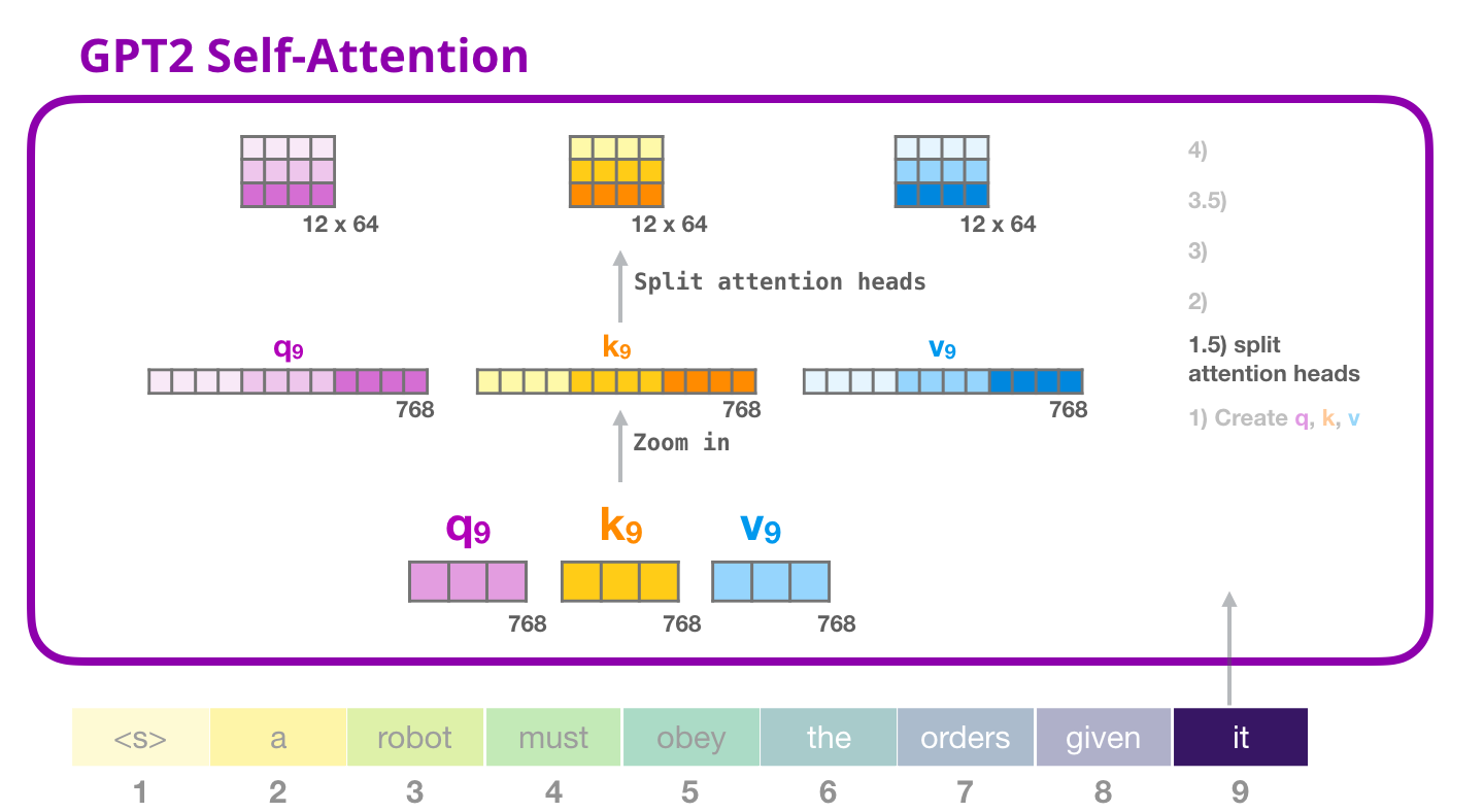
-
Mathematically,
\[\begin{array}{c} h_{i}^{\ell+1}=\text {Concat }\left(\text {head }_{1}, \ldots, \text { head}_{K}\right) O^{\ell} \\ \text { head }_{k}=\text {Attention }\left(Q^{k, \ell} h_{i}^{\ell}, K^{k, \ell} h_{j}^{\ell}, V^{k, \ell} h_{j}^{\ell}\right) \end{array}\]- where \(Q^{k, \ell}, K^{k, \ell}, V^{k, \ell}\) are the learnable weights of the \(k^{\prime}\)-th attention head and \(O^{\ell}\) is a downprojection to match the dimensions of \(h_{i}^{\ell+1}\) and \(h_{i}^{\ell}\) across layers.
-
Multiple heads allow the attention mechanism to essentially ‘hedge its bets’, looking at different transformations or aspects of the hidden features from the previous layer. More on this in the section on Why Multiple Heads of Attention? Why Attention?.
Managing computational load due to multi-head attention
- Unfortunately, multi-head attention really increases the computational load. Computing attention was already the bulk of the work, and we just multiplied it by however many heads we want to use. To get around this, we can re-use the trick of projecting everything into a lower-dimensional embedding space. This shrinks the matrices involved which dramatically reduces the computation time.
- To see how this plays out, we can continue looking at matrix shapes. Tracing the matrix shape through the branches and weaves of the multi-head attention blocks requires three more numbers.
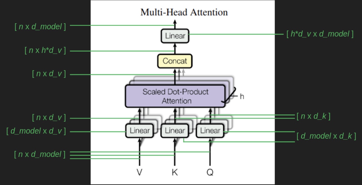
-
The \([n \times d_{model}]\) sequence of embedded words serves as the basis for everything that follows. In each case there is a matrix, \(W_v\), \(W_q\), and \(W_k\), (all shown unhelpfully as “Linear” blocks in the architecture diagram) that transforms the original sequence of embedded words into the values matrix, \(V\), the queries matrix, \(Q\), and the keys matrix, \(K\). \(K\) and \(Q\) have the same shape, \([n \times d_k]\), but \(V\) can be different, \([n \times d_v]\). It confuses things a little that \(d_k\) and \(d_v\) are the same in the paper, but they don’t have to be. An important aspect of this setup is that each attention head has its own \(W_v\), \(W_q\), and \(W_k\) transforms. That means that each head can zoom in and expand the parts of the embedded space that it wants to focus on, and it can be different than what each of the other heads is focusing on.
-
The result of each attention head has the same shape as \(V\). Now we have the problem of h different result vectors, each attending to different elements of the sequence. To combine these into one, we exploit the powers of linear algebra, and just concatenate all these results into one giant \([n \times h * d_v]\) matrix. Then, to make sure it ends up in the same shape it started, we use one more transform with the shape \([h * d_v \times d_{model}]\).
-
Here’s all of the that from the paper, stated tersely.
\[\begin{aligned} \operatorname{MultiHead}(Q, K, V) &=\operatorname{Concat}\left(\operatorname{head}_{1}, \ldots, \text { head }_{\mathrm{h}}\right) W^{O} \\ \text { where head } &=\operatorname{Attention}\left(Q W_{i}^{Q}, K W_{i}^{K}, V W_{i}^{V}\right) \end{aligned}\]- where the projections are parameter matrices \(W_{i}^{Q} \in \mathbb{R}^{d_{\text {model }} \times d_{k}}, W_{i}^{K} \in \mathbb{R}^{d_{\text {model }} \times d_{k}}, W_{i}^{V} \in \mathbb{R}^{d_{\text {model }} \times d_{v}}\) and \(W^{O} \in \mathbb{R}^{h d_{v} \times d_{\text {model }}}\).
Why have multiple attention heads?
- Per Eugene Yan’s Some Intuition on Attention and the Transformer blog, multiple heads lets the model consider multiple words simultaneously. Because we use the softmax function in attention, it amplifies the highest value while squashing the lower ones. As a result, each head tends to focus on a single element.
- Consider the sentence: “The chicken crossed the road carelessly”. The following words are relevant to “crossed” and should be attended to:
- The “chicken” is the subject doing the crossing.
- The “road” is the object being crossed.
- The crossing is done “carelessly”.
- If we had a single attention head, we might only focus on a single word, either “chicken”, “road”, or “crossed”. Multiple heads let us attend to several words. It also provides redundancy, where if any single head fails, we have the other attention heads to rely on.
Cross-Attention
-
The final step in getting the full transformer up and running is the connection between the encoder and decoder stacks, the cross attention block. We’ve saved it for last and, thanks to the groundwork we’ve laid, there’s not a lot left to explain.
-
Cross-attention works just like self-attention with the exception that the key matrix \(K\) and value matrix \(V\) are based on the output of the encoder stack (i.e., the final encoder layer), rather than the output of the previous decoder layer. The query matrix \(Q\) is still calculated from the results of the previous decoder layer. This is the channel by which information from the source sequence makes its way into the target sequence and steers its creation in the right direction. It’s interesting to note that the same embedded source sequence (output from the final layer in the encoder stack) is provided to every layer of the decoder, supporting the notion that successive layers provide redundancy and are all cooperating to perform the same task. The following figure with the Transformer architecture highlights the cross-attention piece within the transformer architecture.
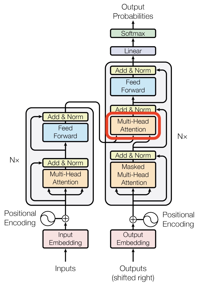
Dropout
- Per the original Transformer paper, dropout is applied to the output of each “sub-layer” (where a “sub-layer” refers to the self/cross multi-head attention layers as well as the position-wise feedfoward networks.), before it is added to the sub-layer input and normalized. In addition, it is also applied dropout to the sums of the embeddings and the positional encodings in both the encoder and decoder stacks. For the base model, the original Transformer use a rate of \(P_{drop} = 0.1\).
- Thus, from a code perspective, the sequence of actions can be summarized as follows:
x2 = SubLayer(x)
x2 = torch.nn.dropout(x2, p=0.1)
x = nn.LayerNorm(x2 + x)
- For more details, please refer The Annotated Transformer.
Skip connections
- Skip connections, introduced in Deep Residual Learning for Image Recognition by He et al. (2015), occur around the Multi-Head Attention blocks, and around the element wise Feed Forward blocks in the blocks labeled “Add and Norm”. In skip connections, a copy of the input is added to the output of a set of calculations. The inputs to the attention block are added back in to its output. The inputs to the element-wise feed forward block are added to its outputs. The following figure shows the Transformer architecture highlighting the “Add and Norm” blocks, representing the residual connections and LayerNorm blocks.
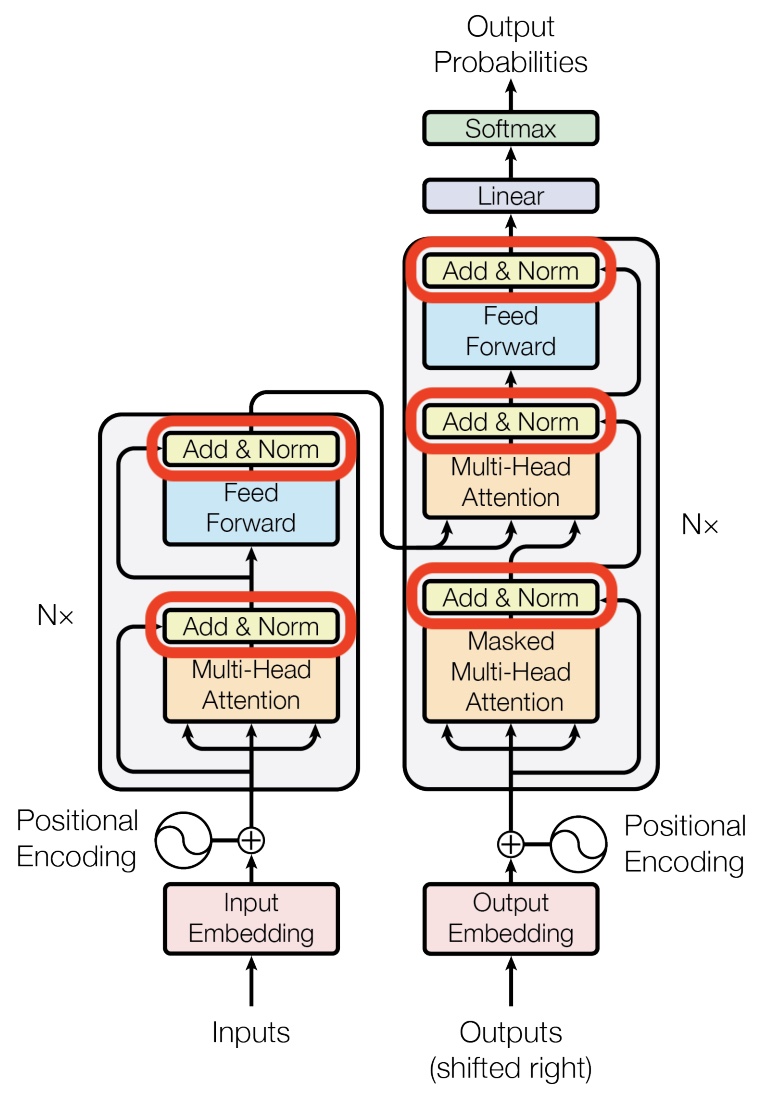
- Skip connections serve two purposes:
- They help keep the gradient smooth, which is a big help for backpropagation. Attention is a filter, which means that when it’s working correctly it will block most of what tries to pass through it. The result of this is that small changes in a lot of the inputs may not produce much change in the outputs if they happen to fall into channels that are blocked. This produces dead spots in the gradient where it is flat, but still nowhere near the bottom of a valley. These saddle points and ridges are a big tripping point for backpropagation. Skip connections help to smooth these out. In the case of attention, even if all of the weights were zero and all the inputs were blocked, a skip connection would add a copy of the inputs to the results and ensure that small changes in any of the inputs will still have noticeable changes in the result. This keeps gradient descent from getting stuck far away from a good solution. Skip connections have become popular because of how they improve performance since the days of the ResNet image classifier. They are now a standard feature in neural network architectures. The figure below (source) shows the effect that skip connections have by comparing a ResNet with and without skip connections. The slopes of the loss function hills are are much more moderate and uniform when skip connections are used. If you feel like taking a deeper dive into how the work and why, there’s a more in-depth treatment in this post. The following diagram shows the comparison of loss surfaces with and without skip connections.
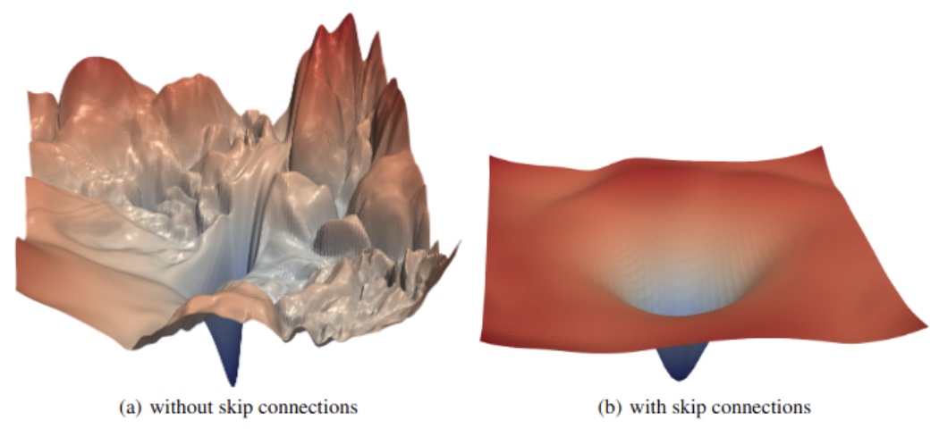
- The second purpose of skip connections is specific to transformers —- preserving the original input sequence. Even with a lot of attention heads, there’s no guarantee that a word will attend to its own position. It’s possible for the attention filter to forget entirely about the most recent word in favor of watching all of the earlier words that might be relevant. A skip connection takes the original word and manually adds it back into the signal, so that there’s no way it can be dropped or forgotten. This source of robustness may be one of the reasons for transformers’ good behavior in so many varied sequence completion tasks.
- They help keep the gradient smooth, which is a big help for backpropagation. Attention is a filter, which means that when it’s working correctly it will block most of what tries to pass through it. The result of this is that small changes in a lot of the inputs may not produce much change in the outputs if they happen to fall into channels that are blocked. This produces dead spots in the gradient where it is flat, but still nowhere near the bottom of a valley. These saddle points and ridges are a big tripping point for backpropagation. Skip connections help to smooth these out. In the case of attention, even if all of the weights were zero and all the inputs were blocked, a skip connection would add a copy of the inputs to the results and ensure that small changes in any of the inputs will still have noticeable changes in the result. This keeps gradient descent from getting stuck far away from a good solution. Skip connections have become popular because of how they improve performance since the days of the ResNet image classifier. They are now a standard feature in neural network architectures. The figure below (source) shows the effect that skip connections have by comparing a ResNet with and without skip connections. The slopes of the loss function hills are are much more moderate and uniform when skip connections are used. If you feel like taking a deeper dive into how the work and why, there’s a more in-depth treatment in this post. The following diagram shows the comparison of loss surfaces with and without skip connections.
Why have skip connections?
- Per Eugene Yan’s Some Intuition on Attention and the Transformer blog, because attention acts as a filter, it blocks most information from passing through. As a result, a small change to the inputs of the attention layer may not change the outputs, if the attention score is tiny or zero. This can lead to flat gradients or local optima.
- Skip connections help dampen the impact of poor attention filtering. Even if an input’s attention weight is zero and the input is blocked, skip connections add a copy of that input to the output. This ensures that even small changes to the input can still have noticeable impact on the output. Furthermore, skip connections preserve the input sentence: There’s no guarantee that a context word will attend to itself in a transformer. Skip connections ensure this by taking the context word vector and adding it to the output.
Layer Normalization
-
Layer Normalization (also called “LayerNorm”) is a technique designed to stabilize and accelerate the training of deep neural networks by normalizing activations within individual samples rather than across batches. It is particularly effective in the Transformer architecture and recurrent architectures, where batch-level statistics are either unavailable or unreliable due to variable sequence lengths or autoregressive processing.
- Relationship with Skip Connections:
- While not inherently dependent on one another, layer normalization often complements skip (residual) connections. Both mechanisms are typically applied after a group of nonlinear computations, such as an attention block or a feed-forward network. Skip connections help preserve gradient flow across layers, and normalization ensures that the magnitude and distribution of activations remain stable, preventing divergence or gradient explosion.
- Conceptual Overview:
-
The essence of layer normalization is to re-center and re-scale the activations of each sample so that they have zero mean and unit variance. Formally, for a layer with hidden dimension \(H\), and activation vector \(x \in \mathbb{R}^{H}\):
\[\mu = \frac{1}{H} \sum_{i=1}^{H} x_i, \quad \sigma^2 = \frac{1}{H} \sum_{i=1}^{H} (x_i - \mu)^2\] \[\hat{x}_i = \frac{x_i - \mu}{\sqrt{\sigma^2 + \epsilon}}, \quad y_i = \gamma_i \hat{x}_i + \beta_i\]- where \(\gamma_i\) and \(\beta_i\) are learnable affine parameters that allow the model to restore representational capacity after normalization.
-
The process ensures that activations remain within a consistent range, which improves numerical stability and gradient propagation across layers.
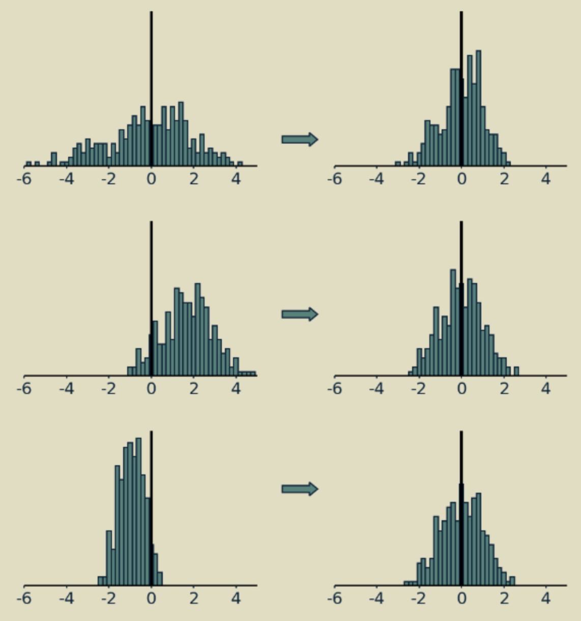
-
- Motivation and Benefits:
-
Deep neural networks, especially those with nonlinear components such as Rectified Linear Units (ReLU) or softmax operators, are highly sensitive to the scale and distribution of intermediate activations. Unlike purely linear systems—where scaling inputs linearly scales outputs—nonlinear architectures can exhibit instability when activations grow or shrink excessively. Layer normalization mitigates this by maintaining stable activation statistics, leading to:
- Faster convergence during training
- Improved generalization and robustness
- Reduced dependence on careful initialization or learning rate tuning
-
This stabilization effect is particularly vital in transformer models, where multiple sub-layers (e.g., attention, feed-forward, and normalization) interact dynamically during training.
-
- Comparison to Other Normalization Methods:
-
Unlike Batch Normalization, which normalizes per channel across the batch dimension and relies on batch-level statistics, layer normalization operates independently for each training example. This makes it well-suited for models with:
- Small or variable batch sizes
- Sequential dependencies (e.g., NLP, speech processing)
- Autoregressive generation tasks
-
For a comprehensive overview of related normalization strategies, including batch, layer, instance, and group normalization, refer to Normalization Methods.
-
Comparison of Normalization Techniques
| Aspect | Layer Normalization (LayerNorm) | Batch Normalization (BatchNorm) | Instance Normalization (InstanceNorm) | Group Normalization (GroupNorm) |
|---|---|---|---|---|
| Normalization Axis | Across all features of a single sample | Across each feature over the entire batch | Across spatial dimensions per channel, per sample | Across groups of channels within each sample |
| Dependency on Batch Size | Independent of batch size | Highly dependent — unreliable for small or varying batches | Independent of batch size | Independent of batch size |
| Statistics Computed Over | Hidden dimension (\(H\)) | Batch dimension (\(B\)) | Spatial dimensions (\(H, W\)) per channel | Subset of channels (groups) within each sample |
| Common Use Cases | Transformers, RNNs, autoregressive models | CNNs, large-batch image models | Style transfer, instance-specific normalization | CNNs with small batches or variable input sizes |
| Inference Behavior | Same as training | Uses running averages (different from training) | Same as training (no running statistics) | Same as training |
| Regularization Effect | Weak | Strong (acts as mild regularizer) | Weak | Moderate |
| Computation Overhead | Low | Moderate (due to batch statistics) | Low | Moderate |
| Stability for Sequential Data | Excellent | Poor | Good | Good |
| Introduced By | Ba et al., 2016 | Ioffe & Szegedy, 2015 | Ulyanov et al., 2016 | Wu & He, 2018 |
-
Guidelines for Use:
-
Use Layer Normalization when:
- Working with transformer architectures (e.g., BERT, GPT, ViT).
- Training with small or variable batch sizes.
- Building models for sequential or autoregressive tasks, such as text generation or speech modeling.
- You need consistent normalization during inference (batch statistics unavailable).
-
Use Batch Normalization when:
- Training CNNs for computer vision with large, consistent batch sizes.
- You want to exploit BatchNorm’s regularizing effect to reduce overfitting.
- The model does not involve temporal dependencies or variable-length sequences.
-
Use Group Normalization when:
- You are training CNNs but have small batch sizes (e.g., object detection, segmentation).
- You want performance similar to BatchNorm without batch dependency.
- You want better spatial feature stability than LayerNorm can provide in convolutional layers.
-
Pre-Norm vs. Post-Norm Transformer Architectures
- The position of the Layer Normalization operation within a Transformer block significantly affects both the training stability and gradient flow. Two common design variants exist: Post-Norm (original Transformer formulation) and Pre-Norm (used in most modern architectures).
- Pre-Norm architectures have become the default design choice for modern Transformer-based models. They enable stable optimization and efficient gradient propagation even in extremely deep networks. However, Post-Norm designs can still be advantageous in smaller or shallower networks where strict output normalization between layers improves consistency.
Post-Norm Transformer (original architecture)
-
In the original Transformer architecture proposed by Vaswani et al. (2017), the normalization layer was applied after the residual connection:
\[x_{l+1} = \text{LayerNorm}(x_l + \text{Sub-block}(x_l))\]- where \(x_l\) is the input to layer \(l\), and Sub-block represents either a multi-head attention block or a feed-forward network.
-
Advantages:
- Output activations are normalized, improving consistency between layers.
- Easy to interpret, as normalization happens at the output of each sub-block.
-
Disadvantages:
- Gradients can vanish or explode in very deep networks because the normalization happens after the residual addition.
- Difficult to train beyond a few dozen layers without specialized initialization or learning rate warm-up.
Pre-Norm Transformer (modern architecture)
- In modern variants (e.g., GPT-2, BERT, T5, LLaMA, DeepSeek–Coder), normalization is applied before the sub-block computation:
-
Advantages:
- Greatly improves training stability and gradient flow — the residual path acts as a direct route for gradients.
- Enables training of very deep transformers (hundreds of layers).
- More robust under different learning rate schedules.
-
Disadvantages:
- The final output of the model may be less normalized, so an additional final LayerNorm is typically applied before the output head.
- May require fine-tuning of initialization to ensure balanced signal scales across layers.
Key Differences
| Aspect | Post-Norm Transformer | Pre-Norm Transformer |
|---|---|---|
| Normalization Placement | After residual addition | Before sub-block computation |
| Gradient Flow | Weakened — gradients pass through normalization | Strong — direct residual path improves gradient stability |
| Training Stability | Poor for deep networks | Excellent, stable for large depth |
| Normalization of Outputs | Each sub-block output normalized | Only input to sub-block normalized |
| Used In | Original Transformer (Vaswani et al., 2017) | BERT, GPT-2/3/4/5, T5, ViT, etc. |
| Need for Final LayerNorm | Optional | Usually required |
Why Transformer Architectures Use Layer Normalization
- Transformers rely heavily on Layer Normalization because of their architectural characteristics and the nature of their training dynamics. LayerNorm plays a crucial role in stabilizing training, maintaining numerical consistency, and ensuring smooth gradient propagation across multiple layers of nonlinear transformations.
- Transformers use Layer Normalization because it provides per-sample, batch-independent, and dimension-consistent normalization. These properties align naturally with the sequential, attention-based, and depth-intensive structure of Transformer models, making LayerNorm not just a practical choice but an architectural necessity for stability and scalability.
How Layer Normalization Works Compared to Batch Normalization
- To fully understand why Transformers rely on Layer Normalization (LayerNorm) instead of Batch Normalization (BatchNorm), it is important to clarify how each operates, what the feature dimension means, and how these differences manifest mathematically and behaviorally.
Normalization Axes and Feature Dimension
-
The feature dimension refers to the set of values that describe a single data point — for example, the hidden vector of one token in a text sequence or the channel vector at one pixel in an image.
- In NLP, an input tensor might have shape
(batch_size, sequence_length, hidden_size).- The feature dimension is hidden_size, meaning each token’s embedding (a vector of hidden_size features) is normalized independently of other tokens and samples.
- In vision models, an input tensor might have shape
(batch_size, height, width, channels).- The feature dimension corresponds to channels — the set of features describing one spatial location.
- In NLP, an input tensor might have shape
-
LayerNorm normalizes across the feature dimension within each individual sample, implying it computes the mean and variance over all features that describe that sample — for instance, the hidden units of a token embedding in a Transformer, or the channels at a single spatial location in a CNN. Each sample is therefore normalized independently of other samples in the batch. This ensures that the normalization depends only on the internal structure of the sample’s feature vector, making LayerNorm invariant to batch composition and consistent between training and inference. As a result, LayerNorm behaves consistently across varying batch sizes, sequence lengths, and between training and inference. This per-sample normalization aligns perfectly with token-based or patch-based architectures like Transformers and Vision Transformers, where each token or patch embedding is treated as an independent feature vector.
-
BatchNorm, on the other hand, normalizes across the batch dimension and, when applicable, across spatial dimensions — for convolutional layers, these are height and width; for Vision Transformers, they correspond to patch tokens within each image. In both cases, for each feature (or channel), BatchNorm computes statistics by aggregating activations from all samples in the batch and all spatial or patch positions. As a result, every activation for a given channel shares the same normalization statistics, introducing dependencies between samples in the batch and between spatial locations within each sample. This coupling across samples and positions can be beneficial in CNNs because it enforces consistent feature statistics across spatial locations and images, helping the network learn stable, spatially coherent feature maps — but it becomes undesirable in Transformers, where each token or patch should be processed independently.
-
While BatchNorm and LayerNorm differ in the axes over which they compute statistics, they are conceptually complementary. BatchNorm normalizes per feature (or channel) across samples in the batch, enforcing consistency of each feature’s distribution across data points. LayerNorm, in contrast, normalizes per sample across all features (or channels), ensuring internal balance within each sample’s representation. Together, they represent two orthogonal views of normalization — one aligning features across data points, the other aligning features within each data point — and some hybrid approaches (such as RMSNorm, GroupNorm, or combined normalization layers) leverage this complementarity to capture benefits of both stability across samples and balance within samples.
Mathematical View
-
Batch Normalization computes mean and variance per feature (e.g., per channel), averaged across all samples in the batch and sometimes across spatial positions:
\[\mu_c = \frac{1}{N \times H \times W} \sum_{n,h,w} x_{n,h,w,c}, \quad \sigma_c^2 = \frac{1}{N \times H \times W} \sum_{n,h,w} (x_{n,h,w,c} - \mu_c)^2\]- where, \(N\) is the batch size, and the normalization for one sample depends on all others in the batch.
-
In contrast, Layer Normalization computes statistics within each sample, across the feature dimension only:
- This means that each token, pixel, or data point is normalized independently of all others.
Practical Implications
-
Because BatchNorm depends on batch-level statistics, its behavior varies with batch size, data distribution, and training mode. It often performs inconsistently during inference when only a single example is available, as it must rely on stored running averages rather than fresh batch statistics.
-
LayerNorm, however, behaves identically during training and inference since it always normalizes each sample in isolation. This makes it perfectly suited for Transformers, where:
- Sequence lengths and batch sizes can vary dramatically.
- Inference is often performed one token at a time (batch size = 1).
- Independence between tokens and batch sequences/samples is required.
Comparison Summary
| Property | Batch Normalization | Layer Normalization |
|---|---|---|
| Normalization axis | Across batch and spatial dimensions (per channel) | Across feature dimensions (per sample) |
| Dependency on batch size | Yes | No |
| Uses running statistics | Yes (for inference) | No |
| Training–inference consistency | Different (depends on stored averages) | Identical |
| Cross-sample dependency | Yes | No |
| Common in | CNNs | Transformers, RNNs |
| Suitable for variable-length input | No | Yes |
Normalization within Transformer Blocks
-
Each Transformer block (layer) consists of two main sub-blocks (sub-layers):
- A multi-head attention mechanism, and
- A position-wise feed-forward network
-
Both are wrapped with residual connections and a normalization layer. LayerNorm helps regulate the scale of activations at each step, preventing either the attention outputs or feed-forward activations from growing uncontrollably.
-
Mathematically, for a pre-norm block:
-
This formulation ensures that even when gradients propagate through hundreds of layers, their magnitudes remain bounded, reducing the likelihood of vanishing or exploding gradients. Specifically, the normalization ensures that the sub-block always operates on inputs with a consistent scale. Because of this:
-
Stable gradient flow: When backpropagating, the gradient through the residual path includes an identity term (from \(x_l\)) and a normalized term (from the sub-block). Since the normalized term has bounded variance, gradients neither amplify (explode) nor diminish (vanish).
-
Well-conditioned transformations: LayerNorm keeps the input distribution to each layer well-conditioned, meaning the local Jacobians of the transformations have singular values near 1. This makes gradient propagation across hundreds of layers stable.
-
Residual smoothing: The residual connection lets gradients bypass the sub-block entirely if necessary, and since the residual stream is normalized, its contribution remains balanced.
- Overall, Pre-Norm ensures that both forward activations and backward gradients stay within predictable ranges, allowing deep transformers (hundreds of layers) to train without special tricks like learning rate warm-up or gradient clipping.
-
Handling Sequential and Autoregressive Computation
-
Transformers often operate in autoregressive or sequence-to-sequence settings, where tokens are processed one at a time during inference. In such scenarios:
- The batch size may be as small as one, especially during text generation.
- The model’s internal activations depend on temporal context rather than parallel samples.
- Because LayerNorm computes normalization statistics over the feature dimension of each individual sample (rather than across the batch), its behavior remains consistent regardless of batch size, sequence length, or whether the model is in training or inference mode.
-
This property is essential for tasks like:
- Language modeling (e.g., GPT series)
- Machine translation (e.g., T5, BERT)
- Speech and vision transformers
Consistent Training and Inference Behavior
- In BatchNorm, statistics computed during training differ from those used during inference — training uses batch statistics, while inference relies on moving averages. This discrepancy can introduce instability if the input distributions change (as often happens in autoregressive or variable-length tasks).
- LayerNorm, on the other hand, computes statistics within each example, ensuring that the behavior during inference is identical to that during training. This alignment significantly simplifies model deployment and evaluation.
Why Transformers Use Layer Normalization vs. Other Forms
-
While several normalization techniques exist, Transformers universally adopt LayerNorm over alternatives like BatchNorm, InstanceNorm, or GroupNorm for the following key reasons:
-
Independence from Batch Statistics
- Layer Normalization operates by computing statistics within each sample, across the hidden (feature) dimension. This means the normalization for a given token or embedding vector does not depend on other samples in the batch.
-
In contrast, Batch Normalization computes the mean and variance across the entire batch for each feature dimension. The equations for BatchNorm are:
\[\mu_j = \frac{1}{B} \sum_{i=1}^{B} x_{ij}, \quad \sigma_j^2 = \frac{1}{B} \sum_{i=1}^{B} (x_{ij} - \mu_j)^2\]- where \(B\) is the batch size.
-
These statistics couple all samples together — the normalization applied to one token depends on every other token in the batch.
- Why BatchNorm doesn’t work here:
- Autoregressive models (like GPT) often operate with batch size = 1 during inference, meaning there is no batch-level variability to compute meaningful statistics.
- Variable-length sequences cause batch elements to have different numbers of tokens, making it challenging to aggregate meaningful feature statistics.
- During training, BatchNorm uses instantaneous batch statistics; during inference, it switches to running averages. In Transformers, the activation distributions can change significantly from training to generation, making these averages unreliable and leading to performance degradation.
-
BatchNorm introduces cross-sample dependencies: each token’s normalization depends on others in the batch, which is undesirable in autoregressive or sequence-dependent processing where each token prediction should be independent of unrelated samples.
- Because of these factors, BatchNorm introduces inconsistency between training and inference phases and instability in sequential models — both of which are unacceptable in Transformer training and deployment.
-
Compatibility with Sequential and Token-wise Processing
- LayerNorm normalizes each token’s embedding vector independently, which aligns with the token-centric computations in the attention mechanism.
- BatchNorm or GroupNorm would introduce dependencies across tokens or samples, violating the independence assumption crucial for attention and autoregressive prediction.
-
Stable Gradient Flow Across Depth
- LayerNorm stabilizes gradients in very deep networks, especially in pre-norm configurations.
- BatchNorm’s reliance on minibatch variance can amplify gradient noise when batch sizes are small or variable.
-
Inference Consistency and Portability
- LayerNorm ensures that inference on single examples behaves identically to training.
- BatchNorm’s need for moving averages of means and variances makes the behavior of the model stateful and potentially inconsistent between training and inference.
-
Empirical Success and Design Simplicity
- Nearly all major Transformer-based architectures — including BERT, GPT-2, T5, and Vision Transformers (ViT) — adopt Layer Normalization as their default. More recent architectures, such as Llama 2, Llama 3, Mistral, Falcon, etc., have transitioned to simplified normalization schemes like RMSNorm, which removes the mean-centering step while preserving the stability and consistency advantages of per-sample normalization.
- Experimental efforts to use Batch Normalization in these contexts (for example, in early attempts to adapt CNN normalization strategies to NLP) often resulted in unstable training, poor convergence, or degraded inference behavior due to the aforementioned statistical dependencies.
-
Related: Modern Normalization Alternatives for Transformers (such as RMSNorm, ScaleNorm, and AdaNorm)
- While LayerNorm remains the dominant normalization technique in Transformer architectures, several recent alternatives have emerged that modify or simplify LayerNorm to improve training efficiency, numerical stability, and scaling behavior for large models. These methods retain LayerNorm’s key benefits—batch-size independence and per-token normalization—while reducing computational overhead or removing dependencies on mean-centering.
Root Mean Square Layer Normalization (RMSNorm)
-
Reference: Zhang & Sennrich, 2019
-
RMSNorm simplifies Layer Normalization by removing the mean-centering step (i.e., the mean subtraction step) and normalizing solely by the root mean square (RMS) of activations.
-
Mathematically, for activations \(x \in \mathbb{R}^{H}\):
\[y = \frac{x}{\text{RMS}(x)} \cdot g, \quad \text{where} \quad \text{RMS}(x) = \sqrt{\frac{1}{H} \sum_{i=1}^{H} x_i^2 + \epsilon}\]- where, \(g\) is a learnable scaling parameter.
-
RMSNorm therefore avoids computing the mean, reducing the number of operations and improving numerical robustness, particularly in mixed-precision (FP16/BF16) training.
-
Advantages:
Scale Normalization (ScaleNorm)
-
Reference: Nguyen & Salazar, 2019
-
ScaleNorm further simplifies normalization by dividing activations by their L2 norm and scaling by a single global parameter \(g\):
\[y = \frac{g \cdot x}{|x|_2}\] -
Unlike LayerNorm or RMSNorm, ScaleNorm does not involve any per-feature affine transformation (\(\gamma, \beta\)) and instead uses a single global scaling factor.
-
Advantages:
- Very lightweight and computationally efficient.
- Maintains stability in deep Transformers.
- Works well in architectures with stable embedding magnitudes, such as language and vision Transformers.
-
Limitations:
- Lacks per-feature learnable flexibility (only a global scaling parameter).
- Slightly less expressive compared to LayerNorm or RMSNorm for heterogeneous feature distributions.
Adaptive Normalization (AdaNorm)
-
Reference: Xu et al., 2019
-
AdaNorm introduces a dynamic, learnable rescaling mechanism that adapts the normalization strength based on the input’s magnitude. It is defined as:
\[y = \frac{x}{\sigma(x)} \cdot \text{sigmoid}(\alpha \sigma(x)) \cdot \gamma + \beta\]- where \(\sigma(x)\) is the standard deviation of activations, and \(\alpha\) is a learnable parameter controlling how strongly normalization is applied.
-
Advantages:
- Reduces over-normalization by allowing the model to adaptively scale features.
- Improves gradient flow and convergence speed, especially in very deep Transformers.
- Demonstrated improvements in both NLP and speech Transformer models.
Comparative Analysis
| Method | Centers Data? | Normalizes by | Learnable Params | Advantages | Common Use Cases |
|---|---|---|---|---|---|
| LayerNorm | Yes (subtracts mean) | Standard deviation | Per-feature (\(\gamma, \beta\)) | Stable, proven, widely supported | Default in all Transformers |
| RMSNorm | No | Root mean square | Per-feature scale (\(g\)) | Faster, numerically stable | Large-scale LLMs (GPT-NeoX, LLaMA) |
| ScaleNorm | No | L2 norm | Single global scale (\(g\)) | Extremely efficient | Lightweight or multilingual models |
| AdaNorm | Yes (adaptive) | Standard deviation | Dynamic scaling (\(\alpha, \gamma, \beta\)) | Learns normalization strength | Deep or dynamically scaled Transformers |
Overall Perspective
- These newer normalization techniques are driven by the scaling challenges of modern Transformer architectures—where models can exceed hundreds of layers and hundreds of billions of parameters.
-
While Layer Normalization remains the most widely adopted, RMSNorm has become increasingly popular in large-scale autoregressive modelssuch as Llama 2, Llama 3, Mistral, Falcon, etc., as it provides equivalent performance with reduced computation and improved stability in mixed-precision environments.
- As a general trend:
Softmax
-
The argmax function is “hard” in the sense that the highest value wins, even if it is only infinitesimally larger than the others. If we want to entertain several possibilities at once, it’s better to have a “soft” maximum function, which we get from softmax. To get the softmax of the value \(x\) in a vector, divide the exponential of \(x\), \(e^x\), by the sum of the exponentials of all the values in the vector. This converts the (unnormalized) logits/energy values into (normalized) probabilities \(\in [0, 1]\), with all summing up to 1.
-
The softmax is helpful here for three reasons. First, it converts our de-embedding results vector from an arbitrary set of values to a probability distribution. As probabilities, it becomes easier to compare the likelihood of different words being selected and even to compare the likelihood of multi-word sequences if we want to look further into the future.
-
Second, it thins the field near the top. If one word scores clearly higher than the others, softmax will exaggerate that difference (owing to the “exponential” operation), making it look almost like an argmax, with the winning value close to one and all the others close to zero. However, if there are several words that all come out close to the top, it will preserve them all as highly probable, rather than artificially crushing close second place results, which argmax is susceptible to. You might be thinking what the difference between standard normalization and softmax is – after all, both rescale the logits between 0 and 1. By using softmax, we are effectively “approximating” argmax as indicated earlier while gaining differentiability. Rescaling doesn’t weigh the max significantly higher than other logits, whereas softmax does due to its “exponential” operation. Simply put, softmax is a “softer” argmax.
-
Third, softmax is differentiable, meaning we can calculate how much each element of the results will change, given a small change in any of the input elements. This allows us to use it with backpropagation to train our transformer.
-
Together the de-embedding transform (shown as the Linear block below) and a softmax function complete the de-embedding process. The following diagram shows the de-embedding steps in the architecture diagram (source: Transformers paper).
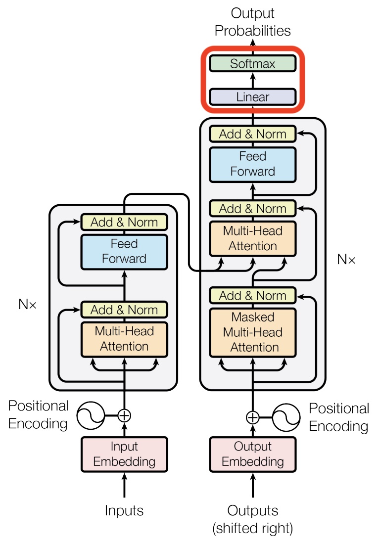
Stacking Transformer Layers
- While we were laying the foundations above, we showed that an attention block and a feed forward block with carefully chosen weights were enough to make a decent language model. Most of the weights were zeros in our examples, a few of them were ones, and they were all hand picked. When training from raw data, we won’t have this luxury. At the beginning the weights are all chosen randomly, most of them are close to zero, and the few that aren’t probably aren’t the ones we need. It’s a long way from where it needs to be for our model to perform well.
- Stochastic gradient descent through backpropagation can do some pretty amazing things, but it relies a lot on trial-and-error. If there is just one way to get to the right answer, just one combination of weights necessary for the network to work well, then it’s unlikely that it will find its way. But if there are lots of paths to a good solution, chances are much better that the model will get there.
- Having a single attention layer (just one multi-head attention block and one feed forward block) only allows for one path to a good set of transformer parameters. Every element of every matrix needs to find its way to the right value to make things work well. It is fragile and brittle, likely to get stuck in a far-from-ideal solution unless the initial guesses for the parameters are very very lucky.
- The way transformers sidestep this problem is by having multiple attention layers, each using the output of the previous one as its input. The use of skip connections make the overall pipeline robust to individual attention blocks failing or giving wonky results. Having multiples means that there are others waiting to take up the slack. If one should go off the rails, or in any way fail to live up to its potential, there will be another downstream that has another chance to close the gap or fix the error. The paper showed that more layers resulted in better performance, although the improvement became marginal after 6.
- Another way to think about multiple layers is as a conveyor belt assembly line. Each attention block and feed-forward block has the chance to pull inputs off the line, calculate useful attention matrices and make next word predictions. Whatever results they produce, useful or not, get added back onto the conveyer, and passed to the next layer. The following diagram shows the transformer redrawn as a conveyor belt:
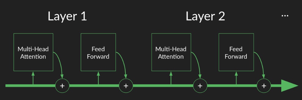
- This is in contrast to the traditional description of many-layered neural networks as “deep”. Thanks to skip connections, successive layers don’t provide increasingly sophisticated abstraction as much as they provide redundancy. Whatever opportunities for focusing attention and creating useful features and making accurate predictions were missed in one layer can always be caught by the next. Layers become workers on the assembly line, where each does what it can, but doesn’t worry about catching every piece, because the next worker will catch the ones they miss.
Why have multiple attention layers?
- Per Eugene Yan’s Some Intuition on Attention and the Transformer blog, multiple attention layers builds in redundancy (on top of having multiple attention heads). If we only had a single attention layer, that attention layer would have to do a flawless job—this design could be brittle and lead to suboptimal outcomes. We can address this via multiple attention layers, where each one uses the output of the previous layer with the safety net of skip connections. Thus, if any single attention layer messed up, the skip connections and downstream layers can mitigate the issue.
- Stacking attention layers also broadens the model’s receptive field. The first attention layer produces context vectors by attending to interactions between pairs of words in the input sentence. Then, the second layer produces context vectors based on pairs of pairs, and so on. With more attention layers, the Transformer gains a wider perspective and can attend to multiple interaction levels within the input sentence.
Transformer Encoder and Decoder
- The Transformer model has two parts: encoder and decoder. Both encoder and decoder are mostly identical (with a few differences) and are comprised of a stack of transformer blocks. Each block is comprised of a combination of multi-head attention blocks, positional feed-forward layers, residual connections and layer normalization blocks.
- The attention layers from the encoder and decoder have the following differences:
- The encoder only has self-attention blocks while the decoder has a cross-attention encoder-decoder layer sandwiched between the self-attention layer and the feed-forward neural network.
- Also, the self-attention blocks are masked to ensure causal predictions (i.e., the prediction of token \(N\) only depends on the previous \(N - 1\) tokens, and not on the future ones).
- Each of the encoding/decoding blocks contains many stacked encoders/decoder transformer blocks. The Transformer encoder is a stack of six encoders, while the decoder is a stack of six decoders. The initial layers capture more basic patterns (broadly speaking, basic syntactic patterns), whereas the last layers can detect more sophisticated ones, similar to how convolutional networks learn to look for low-level features such as edges and blobs of color in the initial layers while the mid layers focus on learning high-level features such as object shapes and textures the later layers focus on detecting the entire objects themselves (using textures, shapes and patterns learnt from earlier layers as building blocks).
- The six encoders and decoders are identical in structure but do not share weights. Check weights shared by different parts of a transformer model for a detailed discourse on weight sharing opportunities within the Transformer layers.
- For more on the pros and cons of the encoder and decoder stack, refer Autoregressive vs. Autoencoder Models.
Decoder stack
The decoder, which follows the auto-regressive property, i.e., consumes the tokens generated so far to generate the next one, is used standalone for generation tasks, such as tasks in the domain of natural language generation (NLG), for e.g., such as summarization, translation, or abstractive question answering. Decoder models are typically trained with an objective of predicting the next token, i.e., “autoregressive blank infilling”.
- As we laid out in the section on Sampling a Sequence of Output Words, the decoder can complete partial sequences and extend them as far as you want. OpenAI created the generative pre-training (GPT) family of models to do just this, by training on a predicting-the-next-token objective. The architecture they describe in this report should look familiar. It is a transformer with the encoder stack and all its connections surgically removed. What remains is a 12 layer decoder stack. The following diagram from the GPT-1 paper Improving Language Understanding by Generative Pre-Training shows the architecture of the GPT family of models:

- Any time you come across a generative/auto-regressive model, such as GPT-X, LLaMA, Copilot, etc., you’re probably seeing the decoder half of a transformer in action.
Encoder stack
The encoder, is typically used standalone for content understanding tasks, such as tasks in the domain of natural language understanding (NLU) that involve classification, for e.g., sentiment analysis, or extractive question answering. Encoder models are typically trained with a “fill in the blanks”/”blank infilling” objective – reconstructing the original data from masked/corrupted input (i.e., by randomly sampling tokens from the input and replacing them with
[MASK]elements, or shuffling sentences in random order if it’s the next sentence prediction task). In that sense, an encoder can be thought of as an auto-encoder which seeks to denoise a partially corrupted input, i.e., “Denoising Autoencoder” (DAE) and aim to recover the original undistorted input.
- Almost everything we’ve learned about the decoder applies to the encoder too. The biggest difference is that there’s no explicit predictions being made at the end that we can use to judge the rightness or wrongness of its performance. Instead, the end product of an encoder stack is an abstract representation in the form of a sequence of vectors in an embedded space. It has been described as a pure semantic representation of the sequence, divorced from any particular language or vocabulary, but this feels overly romantic to me. What we know for sure is that it is a useful signal for communicating intent and meaning to the decoder stack.
-
Having an encoder stack opens up the full potential of transformers instead of just generating sequences, they can now translate (or transform) the sequence from one language to another. Training on a translation task is different than training on a sequence completion task. The training data requires both a sequence in the language of origin, and a matching sequence in the target language. The full language of origin is run through the encoder (no masking this time, since we assume that we get to see the whole sentence before creating a translation) and the result, the output of the final encoder layer is provided as an input to each of the decoder layers. Then sequence generation in the decoder proceeds as before, but this time with no prompt to kick it off.
-
Any time you come across an encoder model that generates semantic embeddings, such as BERT, ELMo, etc., you’re likely seeing the encoder half of a transformer in action.
Putting it all together: The Transformer Architecture
- The Transformer architecture combines the individual encoder/decoder models. The encoder takes the input and encodes it into fixed-length query, key, and vector tensors (analogous to the fixed-length context vector in the original paper by Bahdanau et al. (2015)) that introduced attention. These tensors are passed onto the decoder which decodes it into the output sequence.
-
The encoder (left) and decoder (right) of the transformer is shown below:
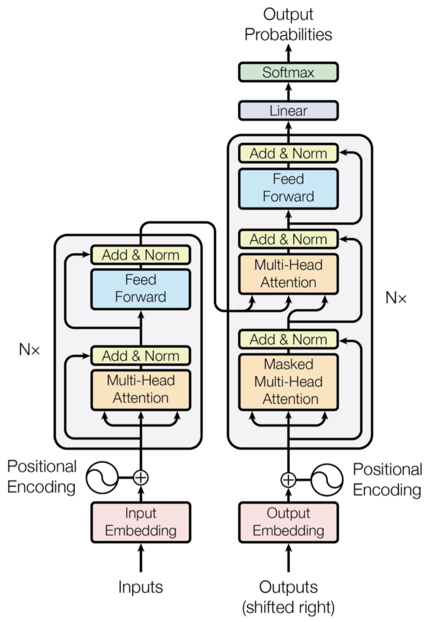
-
Note that the multi-head attention in the encoder is the scaled dot-product multi-head self attention, while that in the initial layer in the decoder is the masked scaled dot-product multi-head self attention and the middle layer (which enables the decoder to attend to the encoder) is the scaled dot-product multi-head cross attention.
-
Re-drawn vectorized versions from DAIR.AI are as follows:
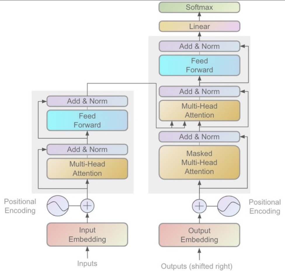
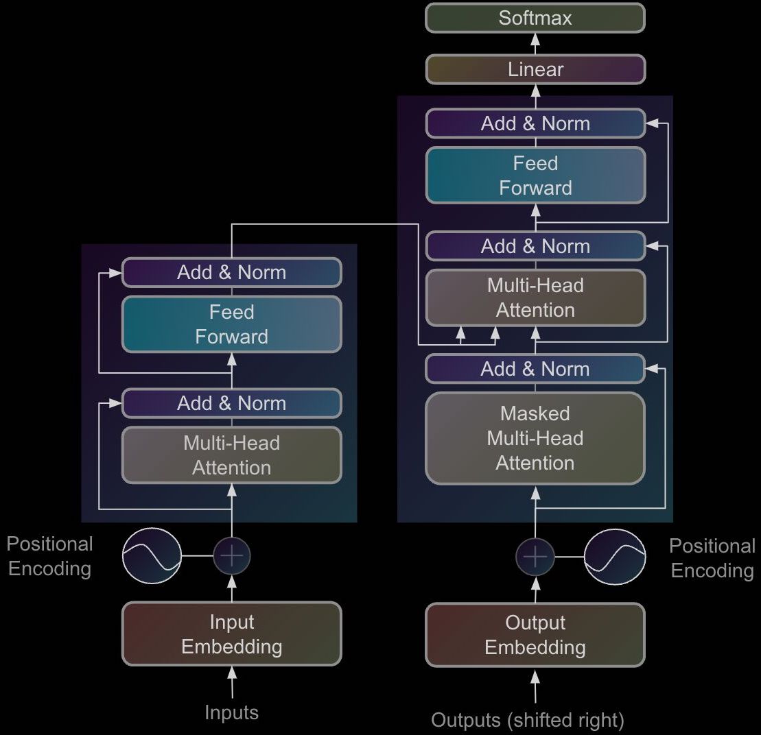
-
- The full model architecture of the transformer – from fig. 1 and 2 in Vaswani et al. (2017) – is as follows:
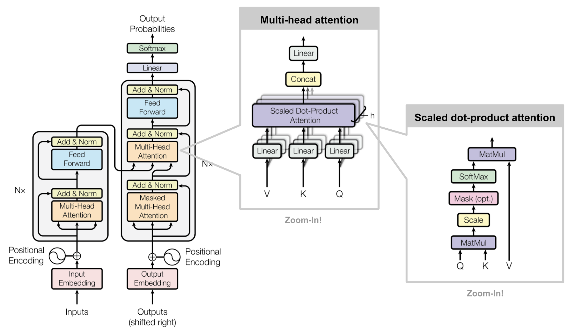
- Here is an illustrated version of the overall Transformer architecture from Abdullah Al Imran:
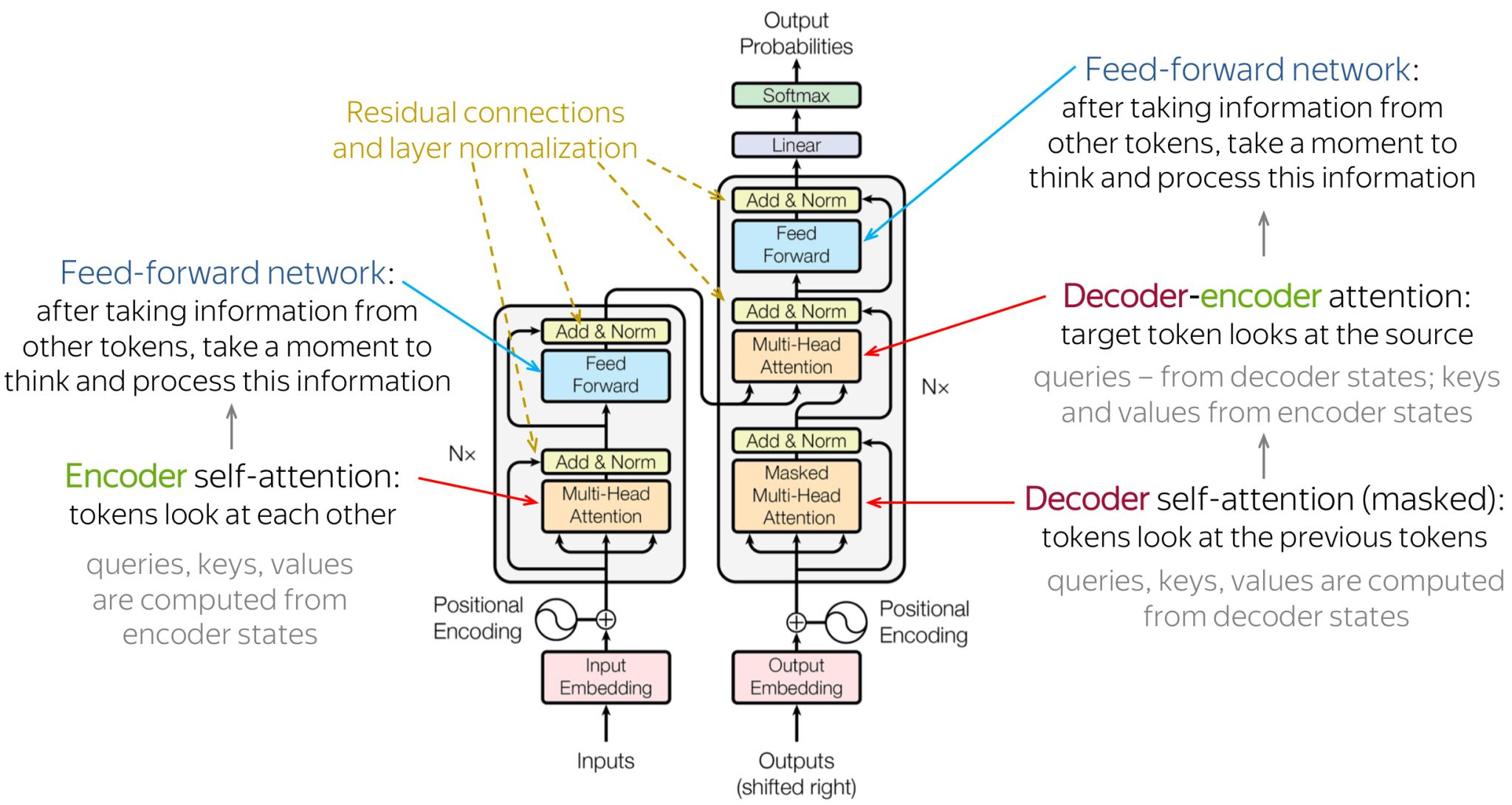
- As a walk-through exercise, the following diagram (source: CS330 slides) shows an sample input sentence “Joe Biden is the US President” being fed in as input to the Transformer. The various transformations that occur as the input vector is processed are:
- Input sequence: \(I\) = “Joe Biden is the US President”.
- Tokenization: \(I \in {\mid \text { vocab } \mid}^{T}\).
- Input embeddings lookup: \(E \in \mathbb{R}^{T \times d}\).
- Inputs to Transformer block: \(X \in \mathbb{R}^{T \times d}\).
- Obtaining three separate linear projections of input \(X\) (queries, keys, and values): \(X_Q=X W_Q, \quad X_K=X W_K, \quad X_V=X W_V\).
- Calculating self-attention: \(A=\operatorname{sm}\left(X_Q X_K^{\top}\right) X_V\) (the scaling part is missing in the figure below – you can reference the section on Types of Attention: Additive, Multiplicative (Dot-product), and Scaled for more).
- This is followed by a residual connection and LayerNorm.
- Feed-forward (MLP) layers which perform two linear transformations/projections of the input with a ReLU activation in between: \(\operatorname{FFN}(x)=\max \left(0, x W_1+b_1\right) W_2+b_2\)
- This is followed by a residual connection and LayerNorm.
- Output of the Transformer block: \(O \in \mathbb{R}^{T \times d}\).
- Project to vocabulary size at time \(t\): \(p_\theta^t(\cdot) \in \mathbb{R}^{\mid \text {vocab } \mid}\).
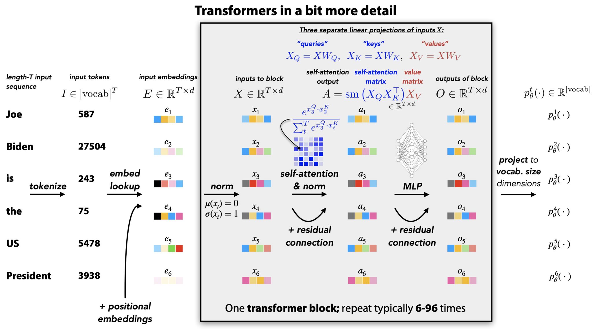
Loss Function
-
Training a Transformer is formulated as an end-to-end optimization problem in which all model parameters are learned jointly by minimizing a differentiable objective function. The standard objective for sequence prediction tasks is the categorical cross-entropy loss, which measures the discrepancy between the model’s predicted probability distributions and the ground-truth target tokens.
-
Consider an output (target) sequence of length \(T\) and a vocabulary of size \(\mid V \mid\). For each output position \(t \in {1, \dots, T}\), the model produces a vector of logits of dimension \(\mid V \mid\). Applying a softmax yields a probability distribution:
\[p_\theta(\cdot \mid \text{context}_t) \in \mathbb{R}^{|V|}\]- where \(\theta\) denotes the model parameters and “context” refers to the information available to the model at position \(t\) (e.g., previous tokens, encoder states).
-
Stacking these distributions across time yields a prediction tensor of shape \([T \times \mid V\mid]\)
-
The ground-truth labels are represented as a length-\(T\) vector of token IDs
\[(y_1, y_2, \dots, y_T)\]- where each \(y_t \in {1, \dots, \mid V\mid}\) indexes the correct vocabulary item at position \(t\).
-
The sequence-level cross-entropy loss is defined as:
- This loss penalizes the model whenever it assigns low probability to the correct token. During backpropagation, gradients of \(\mathcal{L}\) with respect to \(\theta\) are computed and used to update the model weights via gradient-based optimization.
- Importantly, the loss is computed using the normalized softmax probabilities (i.e., the logits after softmax, but prior to any argmax operation). The argmax, which selects the most likely token during inference, is non-differentiable and therefore excluded from training. Minimizing cross-entropy has the effect of continuously increasing the predicted probability of the correct token toward one while decreasing the probabilities assigned to incorrect alternatives, thereby sharpening the model’s predictive distributions over time.
Loss Function Across Architectures
- While the cross-entropy loss provides a common mathematical foundation, its concrete application depends on the Transformer architecture and the learning objective. The distinction lies in which model outputs are compared to ground-truth labels and how context is defined for each prediction.
Encoder-only architectures
-
Encoder-only models (e.g., BERT-style architectures) are not inherently generative. Instead, they are trained to produce rich, bidirectional contextual representations of an input sequence. As a result, the loss is not computed over every position by default, but rather over task-specific subsets of positions.
-
In masked language modeling, a subset of tokens is replaced with a mask symbol or corrupted variants. The encoder processes the entire sequence simultaneously, and the loss is computed only at the masked positions:
\[\mathcal{L} = - \sum_{t \in \mathcal{M}} \log p_\theta(y_t \mid x_{1:T})\]- where \(\mathcal{M}\) denotes the set of masked positions and \(x_{1:T}\) is the full input sequence. This objective encourages the encoder to leverage both left and right context when predicting missing tokens.
-
For classification tasks (e.g., sentence classification), the loss may instead be computed on a single pooled representation (such as a special classification token). In that case, the cross-entropy is applied once per sequence rather than once per token.
Decoder-only architectures
- Decoder-only models (e.g., GPT-style architectures) are trained using an auto-regressive language modeling objective. The loss is computed at every position in the sequence, with each prediction conditioned only on past tokens. This corresponds to maximizing the log-likelihood of the sequence under a causal factorization:
-
The training loss is therefore:
\[\mathcal{L} = - \sum_{t=1}^{T} \log p_\theta(y_t \mid y_{<t})\]- where causal attention masking ensures that the decoder cannot access future tokens. This objective directly aligns training with generation at inference time.
Encoder–decoder (sequence-to-sequence) architectures
-
In encoder–decoder models, the loss is computed exclusively on the decoder outputs, but gradients propagate through both components. The encoder first transforms a source sequence into a sequence of hidden representations. The decoder then generates a target sequence conditioned on:
- previously generated target tokens, and
- the encoder’s output representations via cross-attention.
-
The training objective is:
\[\mathcal{L} = - \sum_{t=1}^{T_{\text{out}}} \log p_\theta(y_t \mid y_{<t}, x_{1:T_{\text{in}}})\]- where \(x_{1:T_{\text{in}}}\) is the source sequence and \(y_{1:T_{\text{out}}}\) is the target sequence. This formulation underlies tasks such as machine translation, summarization, and transcription, enabling joint optimization of source encoding and target generation.
Loss Masking
-
In practical training settings, batches typically contain sequences of variable length. To enable efficient parallel computation, these sequences are padded to a common maximum length. Padding tokens, however, do not represent real data and must not influence the optimization process. Loss masking ensures that such positions contribute neither to the loss value nor to the gradient updates.
-
Let \(T\) denote the padded sequence length and let \(y_t\) be the ground-truth token at position \(t\). Define a binary mask
\[m_t \in {0, 1}\]- where \(m_t = 1\) indicates a valid (non-padding) token and \(m_t = 0\) indicates padding.
-
The masked cross-entropy loss is then written as:
- Positions corresponding to padding tokens are multiplied by zero and therefore contribute neither to the loss nor to the gradients during backpropagation. In many implementations, the loss is additionally normalized by the number of valid tokens to ensure that loss magnitudes remain comparable across batches with different sequence length distributions.
Loss masking and future tokens in decoder-based models
-
In decoder-only and encoder–decoder architectures, loss masking does not apply to future tokens in the same way that attention masking does (cf. Attention Masking). During training, the full target sequence is available (a regime often referred to as teacher forcing). The model is trained to predict every target token \(y_t\), even though it is prevented—via causal attention masking (also known as look-back or triangular attention)—from using information from tokens \(y_{>t}\) when forming that prediction.
-
As a result:
- Future tokens are masked in attention, so they cannot be used as input context.
- Future tokens are not masked in the loss, because they represent valid prediction targets.
-
Each decoder position \(t\) produces a prediction for \(y_t\), conditioned only on past tokens \(y_{<t}\) (and encoder outputs, if present). The loss is therefore computed at all non-padding positions in the target sequence:
\[\mathcal{L} = - \sum_{t=1}^{T_{\text{target}}} \log p_\theta(y_t \mid y_{<t}, \cdot)\]- with masking applied only to padded positions.
Contrast with encoder-only objectives
- In encoder-only models, loss masking may exclude large portions of the sequence depending on the training objective. For example, in masked language modeling, the loss is computed only at masked positions, while unmasked tokens are explicitly excluded from the loss—even though they participate fully in attention.
Loss masking v/s attention masking
-
Loss masking plays a distinct role from attention masking. Attention masking controls the flow of information inside the model by preventing certain positions from attending to others (e.g., future tokens or padding). Loss masking, by contrast, controls the training signal itself, determining which positions contribute to the objective being optimized.
-
The interaction of the two mechanisms is particularly important in decoder and encoder–decoder architectures:
- Attention masking prevents the model from using invalid context,
- Loss masking prevents the model from being penalized for predictions at invalid positions.
-
Together, they ensure that learning is driven solely by meaningful token predictions, preserving both numerical stability and semantic correctness during training.
Implementation details
Tokenization
- Tokenization is a fundamental preprocessing step in NLP, transforming raw text into a sequence of discrete, model-understandable units known as tokens. These tokens may represent words, subwords, characters, or other meaningful linguistic components. In the context of Transformer-based architectures, tokenization serves as the critical bridge between symbolic language and numerical computation. A detailed reference for Transformer implementation nuances can be found in The Annotated Transformer.
Understanding the Role of the Vocabulary
-
As discussed in the section on One-hot encoding, each token in a corpus can be represented by a high-dimensional one-hot vector, with each element corresponding to a unique token in the vocabulary. Constructing such a vocabulary requires knowing a priori which tokens will appear and how many there will be. The vocabulary thus defines the discrete universe in which all textual elements are mapped to numerical identifiers.
-
A naïve approach would be to construct a vocabulary consisting of every possible word in a given language. For English, this could involve tens or even hundreds of thousands of entries, depending on whether inflections, proper nouns, or specialized terminology are included. However, this approach suffers from severe practical and linguistic limitations. The English language is highly productive: it generates plural forms, possessives, and verb conjugations; it includes alternative spellings (e.g., color vs. colour); and it continuously evolves through slang, technical jargon, neologisms, and borrowings from other languages. Furthermore, free-form text data frequently contains typographical errors and inconsistencies in capitalization or punctuation. As a result, an exhaustive list of all possible words would be computationally infeasible and would lead to extreme vocabulary sparsity.
Character-Level Tokenization and Its Limitations
-
An alternative to word-level tokenization is to represent text at the character level. Since the number of unique characters in most writing systems (including punctuation and special symbols) is relatively small, this approach is computationally manageable and language-agnostic. Every character can be encoded as a separate token, allowing the model to theoretically reconstruct any word, including those unseen during training.
-
However, this strategy introduces several problems in practice. In an embedding space, where semantic similarity is encoded as spatial proximity, character-level tokens contain minimal inherent meaning. While words and morphemes often carry semantic or syntactic significance, individual characters generally do not. Consequently, embeddings derived from single characters lack meaningful relationships, resulting in a weak or uninformative semantic geometry.
-
Moreover, Transformer architectures, rely on the principle of self-attention, which models relationships between pairs of tokens rather than strictly preserving their order. When tokenizing at the character level, this mechanism struggles to infer coherent higher-level linguistic structures such as words or phrases, since many relevant character sequences appear indistinguishable once order invariance is partially introduced. Empirical studies have shown that character-level Transformers generally underperform compared to models trained on word- or subword-level representations due to this lack of stable compositional meaning.
Token-to-Character Ratio and Practical Considerations
- According to OpenAI’s Tokenizer documentation, a practical rule of thumb for English text is that one token roughly corresponds to four characters on average, or approximately three-quarters of a word. This implies that 100 tokens represent roughly 75 words. This heuristic is helpful for estimating token counts in applications such as context window sizing, input length budgeting, and computational cost forecasting in LLMs.
Byte Pair Encoding (BPE)
- To overcome the limitations of pure word-level and character-level tokenization, an intermediate approach known as Byte Pair Encoding (BPE) is commonly employed. Originally proposed as a compression algorithm, BPE replaces the most frequent pair of consecutive bytes (or characters) in a dataset with a single, unused byte, effectively merging them into a new symbol. A corresponding lookup table of these merge operations is maintained to enable lossless reconstruction of the original data.
Principle of Operation
-
BPE begins with a base vocabulary consisting of all unique characters in the training corpus, each assigned a distinct code. The algorithm then iteratively identifies the most common adjacent pair of symbols (which may be characters or already-merged subwords) and merges them into a new symbol, assigning it a new code. This merge operation is substituted back into the text, and the process repeats until a predefined number of merge operations—or equivalently, a target vocabulary size—is reached.
-
The resulting subword units can vary in length: frequently occurring sequences such as “trans”, “tion”, or even entire words like “transformer” may be learned as single tokens, while rare or novel words are decomposed into smaller subwords or individual characters. This adaptive vocabulary construction provides a balance between expressiveness and compactness.
Advantages and Modern Implementations
-
BPE enables models to represent both common and rare linguistic patterns effectively. Because it retains the base character set, the tokenizer remains fully capable of representing unseen words, misspellings, or foreign terms without resorting to unknown (UNK) tokens. This makes BPE particularly robust for open-domain language modeling and multilingual corpora.
-
Modern variants of BPE are used extensively across major NLP frameworks. Implementations such as SentencePiece, Hugging Face Tokenizers, and OpenAI’s tiktoken extend BPE principles to handle whitespace, Unicode normalization, and performance optimizations for large-scale corpora. These implementations underpin the preprocessing pipelines of state-of-the-art models such as GPT, BERT, and T5, forming the foundation for efficient and semantically coherent tokenization.
Example
- As an example (credit: Wikipedia: Byte pair encoding), suppose the data to be encoded is:
aaabdaaabac
- The byte pair “aa” occurs most often, so it will be replaced by a byte that is not used in the data, “Z”. Now there is the following data and replacement table:
ZabdZabac
Z=aa
- Then the process is repeated with byte pair “ab”, replacing it with Y:
ZYdZYac
Y=ab
Z=aa
- The only literal byte pair left occurs only once, and the encoding might stop here. Or the process could continue with recursive BPE, replacing “ZY” with “X”:
XdXac
X=ZY
Y=ab
Z=aa
- This data cannot be compressed further by BPE because there are no pairs of bytes that occur more than once.
- To decompress the data, simply perform the replacements in the reverse order.
Applying BPE to Learn New, Rare, and Misspelled Words
- BPE is a subword tokenization algorithm originally proposed for data compression and later adapted for natural language processing (NLP) tasks to efficiently represent variable-length text sequences. The BPE algorithm iteratively merges the most frequent pairs of symbols in a corpus to form new, longer symbols, thereby constructing a vocabulary that balances between word-level and character-level representations. For a detailed exposition of the original method, refer to Sennrich, Haddow, and Birch (2016).
Progressive Construction of Subword Units
-
BPE begins with a base vocabulary consisting of all individual characters in the corpus. Each unique character is treated as an atomic symbol. During training, the algorithm identifies the most frequently co-occurring pair of adjacent symbols (which may be characters or already-merged subwords) and merges them into a new symbol. This process is repeated iteratively, and the resulting merge operations are stored as a sequence of learned “merge rules.”
-
Formally, at each iteration \(t\), the algorithm selects the most frequent pair \((a, b)\) in the corpus and replaces all its occurrences with a new symbol \(ab\). Over time, these merges yield progressively longer subword units that efficiently encode commonly occurring sequences, such as morphemes, roots, or entire words. The length of a subword token is not fixed; it naturally grows to capture recurring linguistic patterns. For instance, the word “transformer” may be represented as a single learned subword token, while a rare or nonsensical string such as
ksowjmckderremains decomposed into smaller units.
Handling Rare and Novel Words
- A major strength of BPE is its ability to generalize to unseen or misspelled words. Because the algorithm preserves the base set of single-character tokens, any new or out-of-vocabulary (OOV) word can still be represented as a sequence of known subword or character tokens. This property allows models using BPE to gracefully handle morphological variations, typographical errors, domain-specific terminology, and even multilingual text. For example, a misspelled word like “transforrmer” could be tokenized into the familiar subwords
transandforrmer, leveraging previously learned components.
Determining Vocabulary Size
- When training a BPE tokenizer, the user specifies a target vocabulary size \(V\). The algorithm continues merging symbol pairs until this limit is reached. Selecting an appropriate \(V\) is critical: a small vocabulary leads to shorter subword units (closer to character-level encoding), while a large vocabulary results in longer tokens (closer to word-level encoding). The goal is to choose \(V\) such that the resulting subword vocabulary captures meaningful semantic and morphological information without excessive fragmentation. Typical vocabulary sizes for Transformer-based models range from 50K to 250K tokens, depending on the language and dataset complexity.
Integration into the Tokenization Pipeline
-
Once trained (or borrowed from a pre-trained model), the BPE tokenizer can be applied to preprocess raw text before it is fed into a Transformer. The tokenizer segments the continuous text stream into a sequence of discrete subword units, each mapped to a unique integer identifier. This transformation enables the model to process text as numerical sequences, facilitating efficient training and inference.
-
This preprocessing stage—known as tokenization—is crucial for modern NLP systems. It ensures consistent segmentation, reduces vocabulary sparsity, and enables fine-grained control over linguistic generalization. Implementations of BPE-based tokenization are widely available in popular NLP libraries, such as Hugging Face Tokenizers, SentencePiece, and OpenAI’s tiktoken.
Comparison with Newer Tokenization Methods
- While BPE remains one of the most influential subword algorithms, several modern alternatives have been developed to address its limitations. The WordPiece algorithm (used in BERT) uses probabilistic likelihood maximization rather than frequency-based merging, which can yield more balanced token boundaries and better coverage for rare words. The Unigram Language Model tokenizer (implemented in SentencePiece) further generalizes this idea by assigning probabilities to all possible subword segmentations and selecting the most likely configuration based on corpus statistics. More recent tokenizers, such as tiktoken, combine BPE-like merges with optimizations for computational efficiency and multilingual robustness. Despite these advancements, BPE’s conceptual simplicity, deterministic nature, and strong empirical performance continue to make it a foundational technique in the Transformer ecosystem.
Teacher Forcing
-
Teacher forcing is a common training technique for sequence-to-sequence architectures, but it applies specifically to the decoder, not to the architecture as a whole. During training, the decoder is fed the ground truth (true) target sequence at each time step as input, rather than its own previous predictions. The encoder does not use teacher forcing because it does not generate tokens autoregressively; it simply encodes the full source sequence. This setup helps the decoder learn faster and more accurately during training because it has access to the correct information at each step.
- Pros: Teacher forcing is essential because it accelerates training convergence and stabilizes learning. By using correct previous tokens as input during training, it ensures the decoder learns to predict the next token accurately. If we do not use teacher forcing, the hidden states of the decoder will be updated by a sequence of wrong predictions, errors will accumulate, making it difficult for the model to learn. This method effectively guides the model in learning the structure and nuances of language (especially during early stages of training when the predictions of the model lack coherence), leading to more coherent and contextually accurate text generation.
- Cons: With teacher forcing, when the model is deployed for inference (generating sequences), it typically does not have access to ground truth information and must rely on its own predictions. Put simply, during inference, since there is usually no ground truth available, the decoder must feed its own previous prediction back to itself for the next prediction. This discrepancy between training and inference can potentially lead to poor model performance and instability. This is known as exposure bias in the literature, which can be mitigated using scheduled sampling.
-
For more, check out What is Teacher Forcing for Recurrent Neural Networks? and What is Teacher Forcing?.
Shift Right (Off-by-One Label Shift) in Decoder Inputs
-
During training with teacher forcing, the Transformer decoder’s inputs must be shifted relative to the target labels so the model learns proper next-token prediction rather than trivially copying the answer.
-
Concretely, a beginning-of-sequence (
BOS) token is prepended to every decoder input sequence. This provides a well-defined start symbol so the model can generate the first token. To keep sequence lengths consistent, the final token of the original target sequence—typically an end-of-sequence (EOS) token or padding (PAD)—is removed. -
If the unshifted target sequence were fed directly into the decoder, the model’s prediction at time step \(t\) would be trained against the label at the same time step \(t\). This would make next-token prediction ill-posed, since the model would be given the very token it is supposed to predict. The shift avoids this leakage.
-
The resulting alignment is:
-
With this setup, each decoder step is trained to predict the next token given all previous ground-truth tokens.
-
This strategy is visually depicted in the Transformer architecture diagram below with the decoder outputs being “shifted right.” Essentially, it prevents the model from “cheating” by seeing the correct output for position \(i\) when predicting position \(i\). In the Transformer decoder diagram below, the input to the decoder at position \(i\) is the correct output token from position \(i-1\). This ensures that when predicting token \(i\), the model can only attend to known outputs from positions less than \(i\), preventing it from “cheating” by seeing the correct token for the current position.
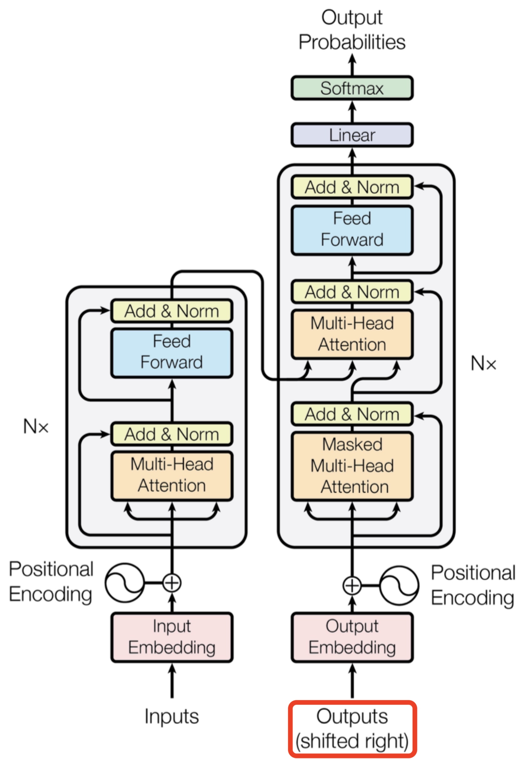
Scheduled Sampling
- Scheduled sampling is a technique used in sequence-to-sequence models, particularly in the context of training recurrent neural networks (RNNs) and sequence-to-sequence models like LSTMs and Transformers. Its primary goal is to address the discrepancy between the training and inference phases that arises due to teacher forcing, and it helps mitigate the exposure bias generated by teacher forcing.
- Scheduled sampling is thus introduced to bridge this “train-test discrepancy” gap between training and inference by gradually transitioning from teacher forcing to using the model’s own predictions during training. Here’s how it works:
- Teacher Forcing Phase:
- In the early stages of training, scheduled sampling follows a schedule where teacher forcing is dominant. This means that the model is mostly exposed to the ground truth target sequence during training.
- At each time step, the model has a high probability of receiving the true target as input, which encourages it to learn from the correct data.
- Transition Phase:
- As training progresses, scheduled sampling gradually reduces the probability of using the true target as input and increases the probability of using the model’s own predictions.
- This transition phase helps the model get accustomed to generating its own sequences and reduces its dependence on the ground truth data.
- Inference Phase:
- During inference (when the model generates sequences without access to the ground truth), scheduled sampling is typically turned off. The model relies entirely on its own predictions to generate sequences.
- Teacher Forcing Phase:
- By implementing scheduled sampling, the model learns to be more robust and capable of generating sequences that are not strictly dependent on teacher-forced inputs. This mitigates the exposure bias problem, as the model becomes more capable of handling real-world scenarios where it must generate sequences autonomously.
- In summary, scheduled sampling is a training strategy for sequence-to-sequence models that gradually transitions from teacher forcing to using the model’s own predictions, helping to bridge the gap between training and inference and mitigating the bias generated by teacher forcing. This technique encourages the model to learn more robust and accurate sequence generation.
Label Smoothing as a Regularizer
- During training, they employ label smoothing which penalizes the model if it gets overconfident about a particular choice. This hurts perplexity, as the model learns to be more unsure, but improves accuracy and BLEU score.
- They implement label smoothing using the KL div loss. Instead of using a one-hot target distribution, we create a distribution that has a reasonably high confidence of the correct word and the rest of the smoothing mass distributed throughout the vocabulary.
Scaling Issues
- A key issue motivating the final Transformer architecture is that the features for words after the attention mechanism might be at different scales or magnitudes. This can be due to some words having very sharp or very distributed attention weights \(w_{i j}\) when summing over the features of the other words. Scaling the dot-product attention by the square-root of the feature dimension helps counteract this issue.
- Additionally, at the individual feature/vector entries level, concatenating across multiple attention heads-each of which might output values at different scales-can lead to the entries of the final vector \(h_{i}^{\ell+1}\) having a wide range of values. Following conventional ML wisdom, it seems reasonable to add a normalization layer into the pipeline. As such, Transformers overcome this issue with LayerNorm, which normalizes and learns an affine transformation at the feature level.
- Finally, the authors propose another ‘trick’ to control the scale issue: a position-wise 2-layer MLP with a special structure. After the multi-head attention, they project \(h_{i}^{\ell+1}\) to a (absurdly) higher dimension by a learnable weight, where it undergoes the ReLU non-linearity, and is then projected back to its original dimension followed by another normalization:
- Since LayerNorm and scaled dot-products (supposedly) didn’t completely solve the highlighted scaling issues, the over-parameterized feed-forward sub-layer was utilized. In other words, the big MLP is a sort of hack to re-scale the feature vectors independently of each other. According to Jannes Muenchmeyer, the feed-forward sub-layer ensures that the Transformer is a universal approximator. Thus, projecting to a very high dimensional space, applying a non-linearity, and re-projecting to the original dimension allows the model to represent more functions than maintaining the same dimension across the hidden layer would. The final picture of a Transformer layer looks like this:
![]()
- The Transformer architecture is also extremely amenable to very deep networks, enabling the NLP community to scale up in terms of both model parameters and, by extension, data. Residual connections between the inputs and outputs of each multi-head attention sub-layer and the feed-forward sub-layer are key for stacking Transformer layers (but omitted from the diagram for clarity).
Adding a New Token to the Tokenizer’s Vocabulary and Model’s Embedding Table
-
When working with pre-trained Transformer models, it is sometimes necessary to introduce new tokens that the tokenizer was not originally trained to recognize. Examples include domain-specific words, symbols, etc. Furthermore, in some cases, it becomes necessary to introduce new special tokens (also known as control tokens)—reserved tokens that perform a specific structural or functional role within a Transformer-based model. Examples include control symbols such as
[PAD],[CLS],[SEP],[MASK], or custom task-oriented tokens like[CONTEXT_START] ... [CONTEXT_END],[NEW_SECTION_START] ... [NEW_SECTION_END], or[DOMAIN_START] ... [DOMAIN_END]. These tokens do not represent natural language words but instead signal boundaries, metadata, or contextual cues that guide model behavior during training and inference. -
Adding a new token involves updating both the tokenizer’s vocabulary and the model’s embedding table so that the new token can be properly represented and learned during fine-tuning.
-
At a top-level, adding a new token to a tokenizer and model involves three coordinated updates:
- Extend the tokenizer’s vocabulary mapping.
- Expand the model’s embedding matrix to include a new row (new token ID).
- If it’s a special token, register the token explicitly as a special token to prevent subword splitting and to ensure consistent treatment across encoding and decoding operations.
- This process ensures the new token becomes a first-class citizen in the model’s lexical and embedding space, capable of being used and learned like any native vocabulary item.
Load the Tokenizer and Model
-
Start by loading your pretrained model and tokenizer:
from transformers import AutoTokenizer, AutoModelForMaskedLM model_name = "bert-base-uncased" tokenizer = AutoTokenizer.from_pretrained(model_name) model = AutoModelForMaskedLM.from_pretrained(model_name) -
Here we use BERT with a masked language modeling (MLM) head as an example. You can use other models (e.g., GPT-2, RoBERTa, etc.) similarly.
Expanding the Tokenizer Vocabulary
- The tokenizer maintains a mapping between text tokens and integer IDs, defined as:
- To add a new token, we simply extend this mapping:
new_token = "[NEW_TOKEN]"
tokenizer.add_tokens([new_token])
- This operation appends the new token to the tokenizer’s internal vocabulary dictionary and assigns it the next available integer ID, e.g.:
- If the original vocabulary had size \(N\), the new vocabulary size becomes \(N + 1\).
Extending the Model’s Embedding Table
-
Each token in the vocabulary has a corresponding vector in the model’s embedding matrix of shape:
\[[N, d_{model}]\]- where \(N\) is the vocabulary size and \(d_{model}\) is the embedding dimension.
-
When a new token is added, we must expand this matrix to accommodate an additional row. This can be achieved using the model’s built-in method:
model.resize_token_embeddings(len(tokenizer)) -
This method performs the following internally:
- Resizes the embedding matrix to shape \([N+1, d_{model}]\).
- Initializes the embedding vector for the new token (row \(N\)) — usually with random values drawn from the same distribution used during model initialization (e.g., uniform or normal with standard deviation proportional to \(\frac{1}{\sqrt{d_{model}}}\)).
-
Thus, the embedding lookup for the new token becomes:
\[E_{new} = W_{E}[N, :]\]- where \(W_{E}\) is the embedding matrix, and the new token’s ID \(N\) indexes its row.
Registering the Token as a Special Token to Prevent Token Splitting
-
If the new token is a special token, a crucial step is to ensure that the tokenizer treats them as indivisible units. If not registered correctly, subword tokenizers like BPE or WordPiece may decompose them into smaller components during text preprocessing.
-
To prevent this, the token must be explicitly declared as a special token:
tokenizer.add_special_tokens({"additional_special_tokens": ["[NEW_TOKEN]"]}) -
This updates the tokenizer’s configuration and internal regular expressions, guaranteeing that
[NEW_TOKEN]is never split or merged with neighboring tokens. Moreover, this ensures consistent behavior across both the encoder and decoder, particularly in sequence-to-sequence architectures. -
Note that this step is only needed for special tokens.
Fine-Tuning the Model to Train the New Embedding
- After successfully integrating the token, it remains untrained until the model encounters it during fine-tuning. To embed the new token meaningfully within the model’s semantic space, fine-tune the model on data where the special token appears in context. The corresponding embedding vector will then evolve under gradient descent to reflect its intended syntactic or functional role.
Practical Considerations
- Adding multiple special tokens at once can be performed by passing a list to
add_special_tokens, after which the model’s embeddings must be resized only once for efficiency. - When loading pre-trained weights, ensure that any newly added tokens do not overwrite existing indices.
- The same tokenizer configuration should always be saved and reloaded alongside the fine-tuned model to maintain token-to-ID consistency.
Extending the Tokenizer to New Languages
- Extending a tokenizer’s vocabulary to cover a new language requires more than simply adding a few tokens. Unlike domain-specific additions, this process typically involves introducing thousands of new subword units to handle the morphology, script, and orthographic rules of the new language. Doing this effectively requires three coordinated steps: expanding the vocabulary, aligning embeddings, and performing multilingual fine-tuning.
- This expanded approach allows a monolingual Transformer model to evolve into a multilingual one without starting from scratch. Through vocabulary expansion, embedding alignment, and multilingual fine-tuning, the model learns to represent new scripts and linguistic structures within a shared semantic space, enabling effective cross-lingual understanding and transfer.
Expanding the Vocabulary with New Subwords
-
For a new language, the tokenizer must learn how to segment words appropriately. Since tokenization strategies like BPE or SentencePiece are data-driven, this involves retraining or augmenting the tokenizer on a corpus representative of the new language.
-
For example, suppose we are extending an English-only tokenizer to also handle Hindi (written in Devanagari). We would first collect a Hindi text corpus and retrain or update the subword model:
from tokenizers import SentencePieceBPETokenizer # Create a new tokenizer and train it on the Hindi corpus tokenizer = SentencePieceBPETokenizer() tokenizer.train( files=["data/hindi_corpus.txt"], vocab_size=52000, min_frequency=2, special_tokens=["<s>", "<pad>", "</s>", "<unk>", "<mask>"] ) -
This process identifies statistically frequent character sequences and merges them into subword tokens that represent the structure of Hindi efficiently. For instance, common units like “क”, “का”, and “में” may become independent subwords, minimizing token fragmentation.
Aligning the New Vocabulary with the Model
-
Once the tokenizer is trained or extended, the model’s embedding table must also be expanded to include the new tokens. If you are extending an existing tokenizer rather than replacing it, the process involves appending the new subwords to the old vocabulary:
# Extend the existing tokenizer and model old_tokenizer.add_tokens(list(new_subwords)) model.resize_token_embeddings(len(old_tokenizer)) -
Each new token receives a randomly initialized embedding vector. However, when adding a related language (for instance, extending an English model to handle Spanish or French), you can partially reuse embeddings for shared characters or subwords.
-
Example:
- The Latin alphabet overlaps across English and Spanish, so the embeddings for “a”, “b”, “c”, etc. can be reused directly.
- Spanish-specific characters like “ñ” or “á”, and subwords like “ción” can be randomly initialized, then refined during fine-tuning.
-
In contrast, when introducing an entirely new script (like Hindi, Chinese, or Arabic), most new tokens will be initialized from scratch. A practical strategy is to initialize these vectors with a small-variance normal distribution centered around the mean of the existing embedding space (i.e., the average of all existing token embedding vectors), helping them start from a meaningful region rather than completely random points. This keeps the new embeddings within the same scale and semantic neighborhood as the pretrained ones, improving stability and convergence during fine-tuning and preventing large gradient jumps that could disrupt already learned representations.
Multilingual Fine-Tuning
After expanding the vocabulary and embedding matrices to include new language-specific tokens, the model must undergo multilingual fine-tuning. This step exposes the Transformer to parallel or comparable multilingual corpora, allowing it to learn shared semantic representations that align meaning across languages. Fine-tuning enables the model to map words, phrases, and syntactic patterns from different languages into a common embedding space, facilitating effective cross-lingual understanding and transfer.
Cross-Lingual Masked Language Modeling (XMLM)
-
The fine-tuning objective typically employs cross-lingual masked language modeling (XMLM), an extension of the traditional masked language modeling (MLM) objective used in monolingual pre-training and first introduced in the XLM paper, Cross-lingual Language Model Pretraining (Conneau & Lample, 2019). In this framework, tokens are randomly masked in sentences drawn from multiple languages, and the model is trained to predict the masked tokens using the surrounding multilingual context.
-
For example, in XMLM, a Swahili sentence like “Watoto wanapenda [MASK] mpira.” (meaning “Children love [MASK] ball.”) might be mixed in the same batch with an English sentence “Children love playing [MASK].”. When predicting the masked token in the Swahili sentence, the model’s self-attention layers can look at all unmasked tokens within that same sentence—for instance, “Watoto” (children), “wanapenda” (love), and “mpira” (ball)—to infer the most likely missing token (“kucheza”, meaning “to play”). Each
[MASK]token’s prediction is conditioned on its intra-sentence context: all surrounding tokens contribute contextual embeddings that flow into the masked position through the attention mechanism. -
Although attention operates independently within each sentence (the Swahili and English examples do not directly attend to one another), mixing sentences from multiple languages in the same batch still promotes implicit cross-lingual alignment through shared parameters and optimization:
- Shared embedding space: All tokens across languages share a single embedding matrix. When the model processes similar contextual patterns—such as “children … love … [MASK] … ball” in English and Swahili—gradient updates push semantically related embeddings (“wanapenda” ↔ “love”, “mpira” ↔ “ball”) closer together.
- Shared model parameters: The same Transformer weights (attention heads and feed-forward layers) are used for all languages. Gradients from different languages jointly update these shared parameters, encouraging the model to encode analogous syntactic and semantic patterns in similar representational subspaces.
- Subword overlap and co-adaptation: Multilingual tokenizers such as SentencePiece or BPE often share subword units across languages. Training on mixed-language batches helps these subword embeddings co-adapt across languages, reinforcing cross-lingual similarity.
-
Over many such batches, the model learns that words or phrases with similar meanings in different languages should occupy neighboring positions in the embedding manifold, even without explicit translation pairs—achieving implicit cross-lingual semantic alignment.
-
Formally, given a multilingual corpus \(\mathcal{D} = { (x^{(l)}, l) }_{l=1}^{L}\), where \(x^{(l)} = (x_1^{(l)}, x_2^{(l)}, \dots, x_T^{(l)})\) represents a token sequence in language \(l\), and \(\mathcal{M}^{(l)} \subseteq {1, \dots, T}\) is the set of masked token indices, the XMLM objective is:
\[\mathcal{L}_{\text{XMLM}} = - \sum_{l=1}^{L} \sum_{i \in \mathcal{M}^{(l)}} \log P \left( x_i^{(l)} \mid x_{\setminus \mathcal{M}^{(l)}}, \theta \right)\]-
where:
- \(L\) denotes the total number of languages;
- \(x_{\setminus \mathcal{M}^{(l)}}\) is the sequence with masked tokens replaced by
[MASK]; - \(\theta\) represents shared model parameters;
- \(P(x_i^{(l)} \mid x_{\setminus \mathcal{M}^{(l)}}, \theta)\) is the predicted probability of the masked token given its multilingual context.
-
-
This cross-lingual MLM objective encourages the model to develop a unified latent space that captures semantic equivalence across languages. Words and phrases with similar meanings are pulled closer together in the embedding manifold, regardless of linguistic form.
Translation Language Modeling (TLM)
-
In practice, large multilingual models such as XLM and XLM-R use XMLM for pre-training across 100+ languages. The Translation Language Modeling (TLM) objective, also introduced in the same XLM paper, extends this idea to parallel corpora (translated sentence pairs), enabling explicit cross-lingual supervision.
-
When parallel sentences are available, TLM concatenates the source and target sentences, masks tokens in both, and forces the model to predict masked words using cross-sentence attention—allowing each masked token to look not only at its own sentence but also at its translation.
-
For example, the model might see: “The cat is [MASK] the table. [SEP] Le chat est [MASK] la table.” Here, when predicting “under” in English, the model can attend to “sous” in the French sentence, and vice versa. This bidirectional information flow allows the model to explicitly align semantically equivalent words across languages.
-
Formally, the TLM objective is:
-
where \(x\) and \(y\) denote the source and target sentences, and \(\mathcal{M}\) is the set of masked token positions across both. This objective encourages the model to use bilingual context when reconstructing masked tokens, fostering explicit alignment between languages.
-
While XMLM relies on independent monolingual data and achieves implicit alignment through shared representations and multilingual co-training, TLM leverages direct bilingual supervision to produce explicit alignment, reinforcing that words and phrases with similar meanings in different languages occupy nearby positions in the model’s embedding space.
Detailed Example of Multilingual Fine-Tuning
-
Suppose we are extending a pre-trained English BERT model to include Spanish and Hindi. The process would look like this:
-
Data Preparation:
- Collect corpora in English, Spanish, and Hindi (e.g., Wikipedia dumps, news text, or parallel translation datasets).
- Tokenize using the newly extended tokenizer that includes tokens for all three languages.
-
Mix the datasets together, ensuring a balance between high- and low-resource languages by adjusting sampling ratios.
-
Example corpus samples:
  English: The weather is pleasant today.
  Spanish: El clima es agradable hoy.
  Hindi: आज का मौसम सुहावना है।
(English) The cat is sleeping. (Spanish) El gato está durmiendo. (Hindi) बिल्ली सो रही है।
-
Training Setup:
- Use a multilingual MLM objective with random masking of tokens (typically 15%).
-
Mask tokens from all languages in a shared batch, forcing the model to learn a unified representation space.
-
Example masked sequences:
  English: The [MASK] is pleasant today.
  Spanish: El clima es [MASK] hoy.
  Hindi: आज का [MASK] सुहावना है।
(English) The [MASK] is sleeping. (Spanish) El [MASK] está durmiendo. (Hindi) [MASK] सो रही है। - During training, the model must predict the masked token from context in its respective language, while also sharing parameters across languages.
-
Cross-Lingual Masked Language Modeling:
- Using the translation pairs or parallel sentences, align semantics between languages by performing cross-lingual masked language modeling (predicting masked tokens). For example, train on the aforementioned English–Spanish-Hindi triplets where all sentences express the same meaning.
- The model learns to produce similar embeddings for equivalent words or phrases across languages.
-
Task-Specific Multilingual Fine-Tuning:
-
Once cross-lingual MLM converges, the model can be fine-tuned for specific tasks such as:
- Multilingual Question Answering (e.g., XQuAD, TyDiQA)
- Natural Language Inference (e.g., XNLI)
- Sentiment Analysis across languages.
-
Example for sentiment classification:
- Input: “El servicio fue excelente.” (Spanish)
- Output: Positive sentiment (aligned with “The service was excellent.” in English).
-
-
Regularization and Data Balancing:
- Use sampling temperature to upsample underrepresented languages like Hindi to prevent overfitting on dominant languages such as English.
- Apply embedding regularization to stabilize learning of new tokens.
- Gradually unfreeze layers during multilingual fine-tuning to maintain prior knowledge while adapting to new languages.
-
End-to-end flow: from input embeddings to next-token prediction
- This section gives a detailed, dimension-aware walk-through of how an autoregressive, post-layer-norm Transformer processes a sequence of input tokens, from input embeddings through attention and feed-forward transformations to next-token prediction and efficient generation.
Step 1: Tokenization \(\rightarrow\) token IDs
- Raw text is converted by a tokenizer into a sequence of token IDs:
- For a batch of size \(B\), this has shape \((B, T)\).
Step 2: Token embeddings and positional encoding
- Each token ID is mapped to a learned embedding vector using an embedding matrix:
-
This yields token embeddings:
\[e_t = E[x_t] \in \mathbb{R}^{d_{model}}\]- … and a tensor of shape \((B, T, d_{model})\).
-
Positional information is incorporated so the model can represent order. This may be done by adding learned positional embeddings to the token embeddings or by injecting position information inside attention (for example via rotary embeddings). After this step, the initial hidden representation is:
Step 3: Stack of \(L\) Transformer decoder layers
-
The model applies \(L\) identical decoder layers. Each layer preserves the shape \((B, T, d_{model})\) while progressively contextualizing the representations.
-
In post-norm architectures (such as the original Transformer), each sublayer is followed by a residual connection and then a layer normalization.
Step 3.1: Masked multi-head self-attention
-
The input to layer \(\ell\) is \(H^{(\ell-1)}\)
-
Linear projections produce queries, keys, and values:
\[Q = H^{(\ell-1)} W_Q,\quad K = H^{(\ell-1)} W_K,\quad V = H^{(\ell-1)} W_V\]-
with:
\[W_Q, W_K, W_V \in \mathbb{R}^{d_{model}\times d_{model}}\]
-
-
These tensors are reshaped into \(h\) attention heads, each with head dimension:
- For each position \(t\), scaled dot-product attention is computed over positions \(i \le t\):
- A causal mask prevents attention to future positions. After applying softmax to obtain attention weights, the output at position \(t\) is:
- Outputs from all attention heads are first concatenated to form a vector of size \(d_{model}\) and are then linearly mixed using the following output projection which linearly mixes information across heads (without changing dimensionality), enabling interaction between features learned by different attention heads:
- A residual connection and post-norm are applied:
Step 3.2: Feed-forward network
-
The feed-forward network is applied independently at each sequence position:
\[\text{FFN}(x) = W_2 \sigma(W_1 x + b_1) + b_2\]-
where:
\[W_1 \in \mathbb{R}^{d_{ff}\times d_{model}},\quad W_2 \in \mathbb{R}^{d_{model}\times d_{ff}}\]-
with:
\[d_{ff} = 4 d_{model} \quad \text{(in standard GPT-style models)}\]
-
-
-
This sublayer first expands the representation from \(d_{model}\) to a higher-dimensional space \(d_{ff}\), applies a non-linearity, and then projects the result back down to \(d_{model}\), allowing the model to perform richer per-token transformations while keeping the overall model width fixed.
-
A residual connection and post-norm complete the layer:
- After all \(L\) layers, the output is
Step 4: Select the final token representation
- To predict the next token, the model uses only the hidden state at the last position:
- This vector summarizes the entire prefix via masked self-attention.
Step 5: Projection to vocabulary logits
-
The final hidden state is mapped to vocabulary logits:
\[\text{logits} = h_{last} W_{vocab} + b_{vocab}\]-
where:
\[W_{vocab} \in \mathbb{R}^{d_{model}\times |\mathcal{V}|}\]
-
-
In many implementations, \(W_{vocab}\) is tied to the input embedding matrix \(E^\top\) (via weight tying).
Step 6: Softmax and token selection
- A softmax converts logits into a probability distribution over the vocabulary:
- A decoding strategy (greedy, temperature sampling, top-\(k\), or nucleus sampling) selects the next token.
Step 7: Autoregressive generation loop
- The selected token is appended to the existing sequence, forming a longer prefix. The entire forward process is then repeated to predict the following token. This autoregressive loop continues until a stopping condition is met (for example, an end-of-sequence token or a maximum length).
Step 8: Key–value (KV) caching for efficient inference
-
During inference, efficiency is improved by caching the key and value tensors produced by the self-attention sublayer at each transformer layer.
-
For a given layer \(\ell\), the cached tensors have shapes:
-
When generating a new token at position \(T+1\):
- Only the new token’s query \(Q_{T+1}\) (and its corresponding key and value) is computed.
- Attention is performed between \(Q_{T+1}\) and the cached keys \(K^{(\ell)}_{\text{cache}}\), and the cached values are used to form the context vector.
-
This avoids recomputing attention for all previous tokens at every step, reducing the per-token computational cost from quadratic in sequence length to linear, which is critical for fast autoregressive decoding.
-
A detailed discourse of KV caching is available in our Model Acceleration primer.
The relation between transformers and Graph Neural Networks
GNNs build representations of graphs
-
Let’s take a step away from NLP for a moment.
-
Graph Neural Networks (GNNs) or Graph Convolutional Networks (GCNs) build representations of nodes and edges in graph data. They do so through neighbourhood aggregation (or message passing), where each node gathers features from its neighbours to update its representation of the local graph structure around it. Stacking several GNN layers enables the model to propagate each node’s features over the entire graph—from its neighbours to the neighbours’ neighbours, and so on.
-
Take the example of this emoji social network below (source): The node features produced by the GNN can be used for predictive tasks such as identifying the most influential members or proposing potential connections.
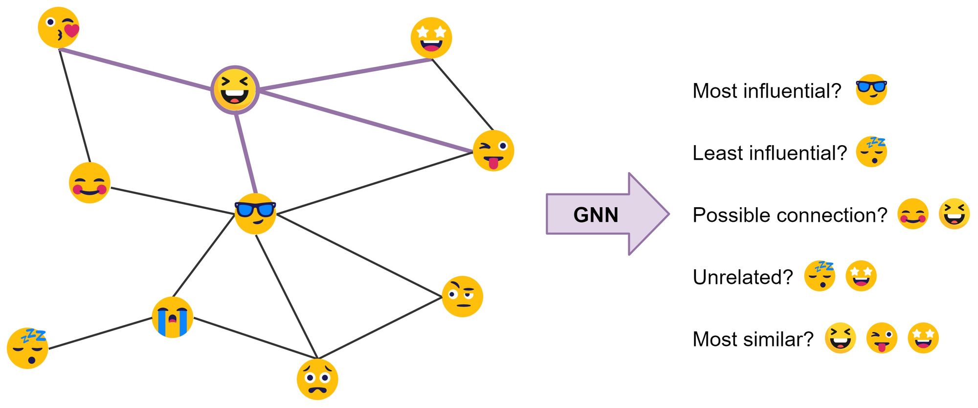
-
In their most basic form, GNNs update the hidden features \(h\) of node \(i\) (for example, 😆) at layer \(\ell\) via a non-linear transformation of the node’s own features \(h_{i}^{\ell}\) added to the aggregation of features \(h_{j}^{\ell}\) from each neighbouring node \(j \in \mathcal{N}(i)\):
\[h_{i}^{\ell+1}=\sigma\left(U^{\ell} h_{i}^{\ell}+\sum_{j \in \mathcal{N}(i)}\left(V^{\ell} h_{j}^{\ell}\right)\right)\]- where \(U^{\ell}, V^{\ell}\) are learnable weight matrices of the GNN layer and \(\sigma\) is a non-linear function such as ReLU. In the example, (😆) {😘, 😎, 😜, 🤩}.
-
The summation over the neighbourhood nodes \(j \in \mathcal{N}(i)\) can be replaced by other input sizeinvariant aggregation functions such as simple mean/max or something more powerful, such as a weighted sum via an attention mechanism.
-
Does that sound familiar? Maybe a pipeline will help make the connection (figure source):
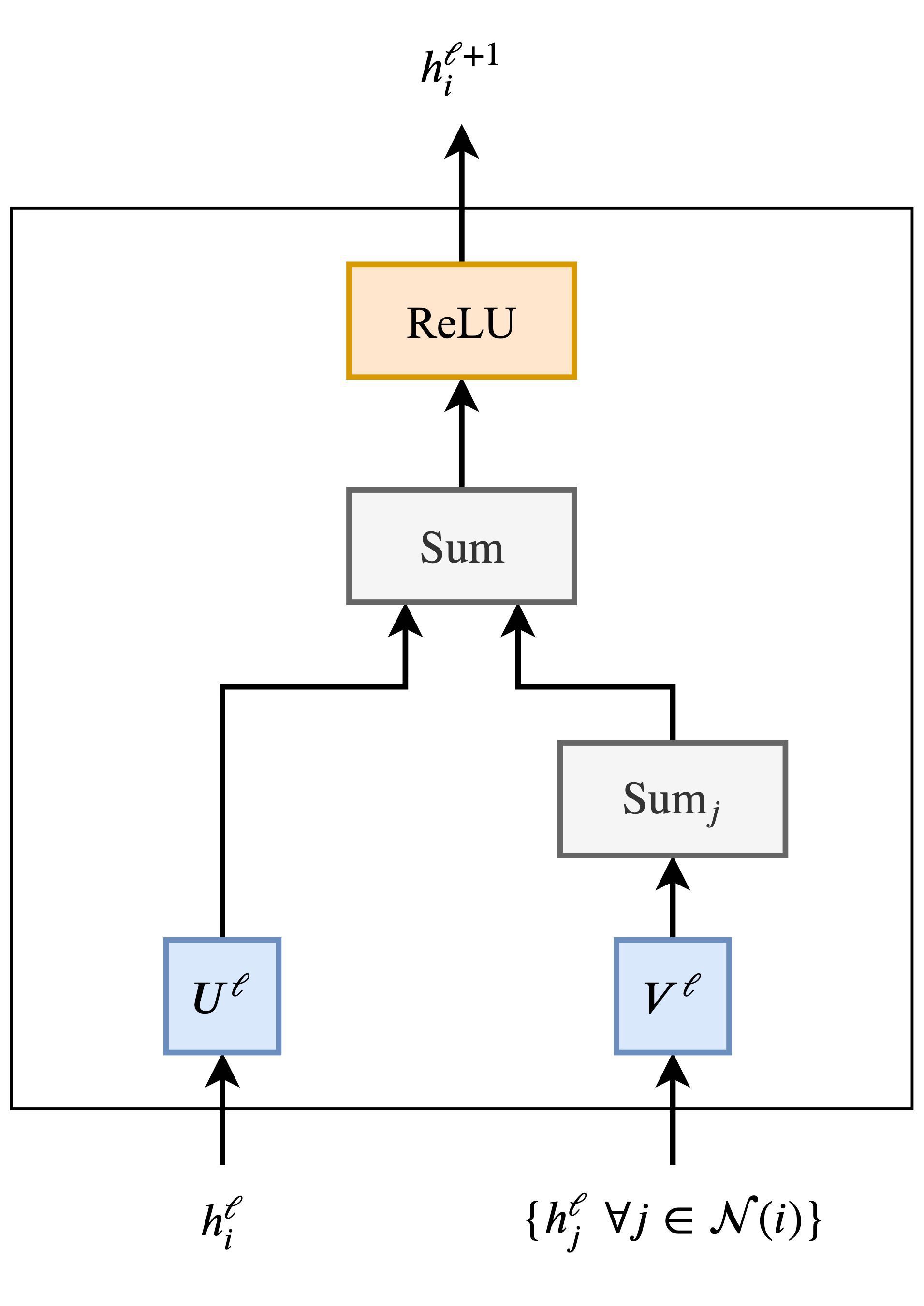
- If we were to do multiple parallel heads of neighbourhood aggregation and replace summation over the neighbours \(j\) with the attention mechanism, i.e., a weighted sum, we’d get the Graph Attention Network (GAT). Add normalization and the feed-forward MLP, and voila, we have a Graph Transformer! Transformers are thus a special case of GNNs – they are just GNNs with multi-head attention.
Sentences are fully-connected word graphs
- To make the connection more explicit, consider a sentence as a fully-connected graph, where each word is connected to every other word. Now, we can use a GNN to build features for each node (word) in the graph (sentence), which we can then perform NLP tasks with as shown in the figure (source) below.
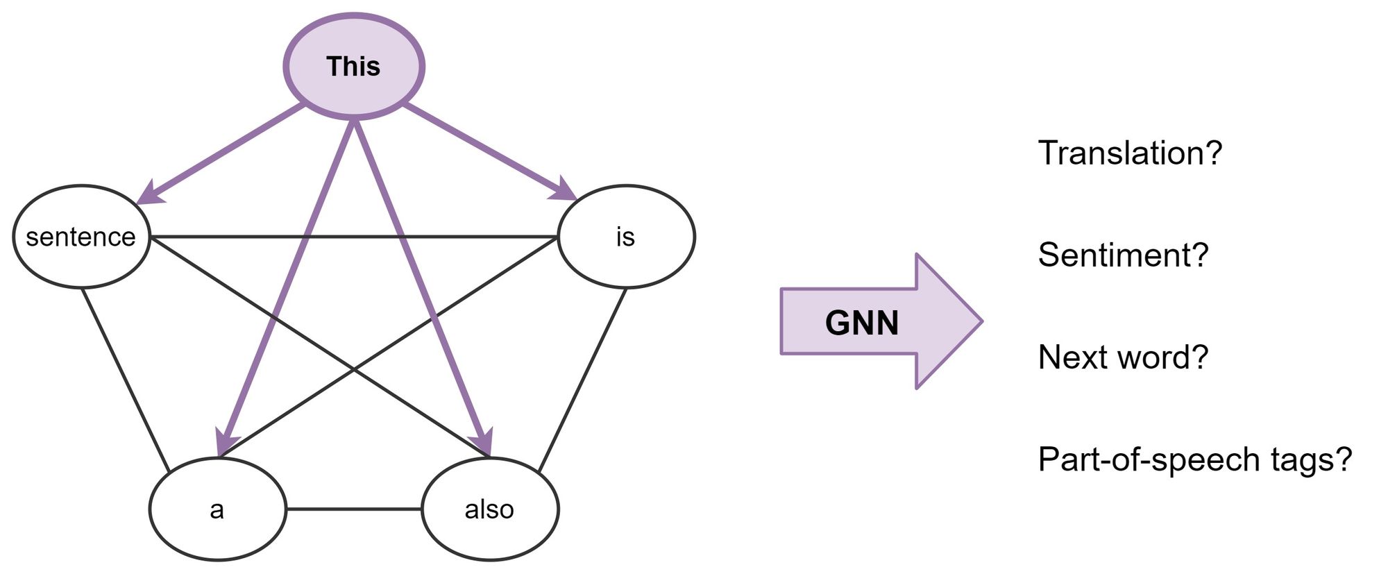
-
Broadly, this is what Transformers are doing: they are GNNs with multi-head attention as the neighbourhood aggregation function. Whereas standard GNNs aggregate features from their local neighbourhood nodes \(j \in \mathcal{N}(i)\), Transformers for NLP treat the entire sentence \(\mathcal{S}\) as the local neighbourhood, aggregating features from each word \(j \in \mathcal{S}\) at each layer.
-
Importantly, various problem-specific tricks—such as position encodings, causal/masked aggregation, learning rate schedules and extensive pre-training—are essential for the success of Transformers but seldom seem in the GNN community. At the same time, looking at Transformers from a GNN perspective could inspire us to get rid of a lot of the bells and whistles in the architecture.
Inductive biases of transformers
- Based on the above discussion, we’ve established that transformers are indeed a special case of Graph Neural Networks (GNNs) owing to their architecture level commonalities. Relational inductive biases, deep learning, and graph networks by Battaglia et al. (2018) from DeepMind/Google, MIT and the University of Edinburgh offers a great overview of the relational inductive biases of various neural net architectures, summarized in the table below from the paper. Each neural net architecture exhibits varying degrees of relational inductive biases. Transformers fall somewhere between RNNs and GNNs in the table below (source).
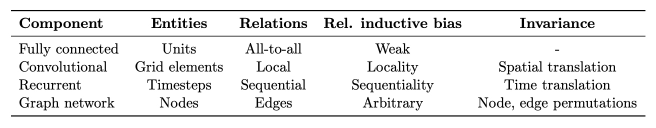
- YouTube Video from UofT CSC2547: Relational inductive biases, deep learning, and graph networks; Slides by KAIST on inductive biases, graph neural networks, attention and relational inference
Time complexity: RNNs vs. Transformers
- RNNs and Transformers have different time complexities, which significantly impact their runtime performance, especially on long sequences. This section offers a detailed explanation of the time complexities of RNNs and Transformers, including the reasoning behind each term in the complexities.
RNNs
- Time Complexity: \(O(n \cdot d^2)\)
- Explanation:
- \(n\): This represents the length of the input sequence. RNNs process sequences one step at a time, so they need to iterate through all \(n\) time steps.
- \(d\): This represents the dimensionality of the hidden state.
- \(d^2\): This term arises because at each time step, an RNN performs operations that involve the hidden state. Specifically, each step involves matrix multiplications that have a computational cost of \(O(d^2)\). The key operations are:
- Hidden State Update: For a simple RNN, the hidden state update is computed as \(h_t = \tanh(W_h h_{t-1} + W_x x_t)\). Here, \(W_h\) and \(W_x\) are weight matrices of size \(d \times d\) and \(d \times n\), respectively.
- The matrix multiplication \(W_h h_{t-1}\) dominates the computation and contributes \(O(d^2)\) to the complexity because multiplying a \(d \times d\) matrix with a \(d\)-dimensional vector requires \(d^2\) operations.
- Therefore, for each of the \(n\) time steps, the \(d^2\) operations need to be performed, leading to the overall time complexity of \(O(n \cdot d^2)\).
- Explanation:
Transformers
- Time Complexity: \(O(n^2 \cdot d)\)
- Explanation:
- \(n\): This represents the length of the input sequence.
- \(n^2\): This term arises from the self-attention mechanism used in Transformers. In self-attention, each token in the sequence attends to every other token, requiring the computation of attention scores for all pairs of tokens. This results in \(O(n^2)\) pairwise comparisons.
- \(d\): This represents the dimensionality of the model. The attention mechanism involves projecting the input into query, key, and value vectors of size \(d\), and computing dot products between queries and keys, which are then scaled and used to weight the values. The operations involved are:
- Projection: Each input token is projected into three different \(d\)-dimensional spaces (query, key, value), resulting in a complexity of \(O(nd)\) for this step.
- Dot Products: Computing the dot product between each pair of query and key vectors results in \(O(n^2 d)\) operations.
- Weighting and Summing: Applying the attention weights to the value vectors and summing them up also involves \(O(n^2 d)\) operations.
- Therefore, the overall time complexity for the self-attention mechanism in Transformers is \(O(n^2 \cdot d)\).
- Explanation:
Comparative Analysis
- RNNs: The linear time complexity with respect to the sequence length makes RNNs potentially faster for shorter sequences. However, their sequential nature can make parallelization challenging, leading to slower processing times for long sequences on modern hardware optimized for parallel computations. Put simply, the dependency on previous time steps means that RNNs cannot fully leverage parallel processing, which is a significant drawback on modern hardware optimized for parallel computations.
- Transformers: The quadratic time complexity with respect to the sequence length means that Transformers can be slower for very long sequences. However, their highly parallelizable architecture often results in faster training and inference times on modern GPUs, especially for tasks involving long sequences or large datasets. This parallelism makes them more efficient in practice, especially for tasks involving long sequences or large datasets. The ability to handle dependencies across long sequences without being constrained by the sequential nature of RNNs gives Transformers a significant advantage in many applications.
Practical Implications
- For tasks involving short to moderately long sequences, RNNs can be efficient and effective.
- For tasks involving long sequences, Transformers are generally preferred due to their parallel processing capabilities, despite their higher theoretical time complexity.
Summary
- RNNs: \(O(n \cdot d^2)\) – Efficient for shorter sequences, but limited by sequential processing.
- Transformers: \(O(n^2 \cdot d)\) – Better suited for long sequences due to parallel processing capabilities, despite higher theoretical complexity.
Lessons Learned
Transformers: merging the worlds of linguistic theory and statistical NLP using fully connected graphs
-
Now that we’ve established a connection between Transformers and GNNs, let’s throw some ideas around. For one, are fully-connected graphs the best input format for NLP?
-
Before statistical NLP and ML, linguists like Noam Chomsky focused on developing formal theories of linguistic structure, such as syntax trees/graphs. Tree LSTMs already tried this, but maybe Transformers/GNNs are better architectures for bringing together the two worlds of linguistic theory and statistical NLP? For example, a very recent work from MILA and Stanford explores augmenting pre-trained Transformers such as BERT with syntax trees [Sachan et al., 2020. The figure below from Wikipedia: Syntactic Structures shows a tree diagram of the sentence “Colorless green ideas sleep furiously”:
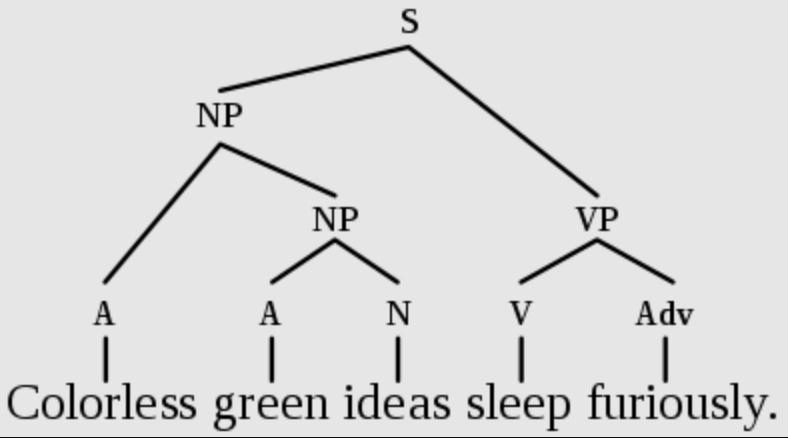
Long term dependencies
-
Another issue with fully-connected graphs is that they make learning very long-term dependencies between words difficult. This is simply due to how the number of edges in the graph scales quadratically with the number of nodes, i.e., in an \(n\) word sentence, a Transformer/GNN would be doing computations over \(n^{2}\) pairs of words. Things get out of hand for very large \(n\).
-
The NLP community’s perspective on the long sequences and dependencies problem is interesting: making the attention mechanism sparse or adaptive in terms of input size, adding recurrence or compression into each layer, and using Locality Sensitive Hashing for efficient attention are all promising new ideas for better transformers. See Maddison May’s excellent survey on long-term context in Transformers for more details.
-
It would be interesting to see ideas from the GNN community thrown into the mix, e.g., Binary Partitioning for sentence graph sparsification seems like another exciting approach. BP-Transformers recursively sub-divide sentences into two until they can construct a hierarchical binary tree from the sentence tokens. This structural inductive bias helps the model process longer text sequences in a memory-efficient manner. The following figure from Ye et al. (2019) shows binary partitioning for sentence graph sparsification.
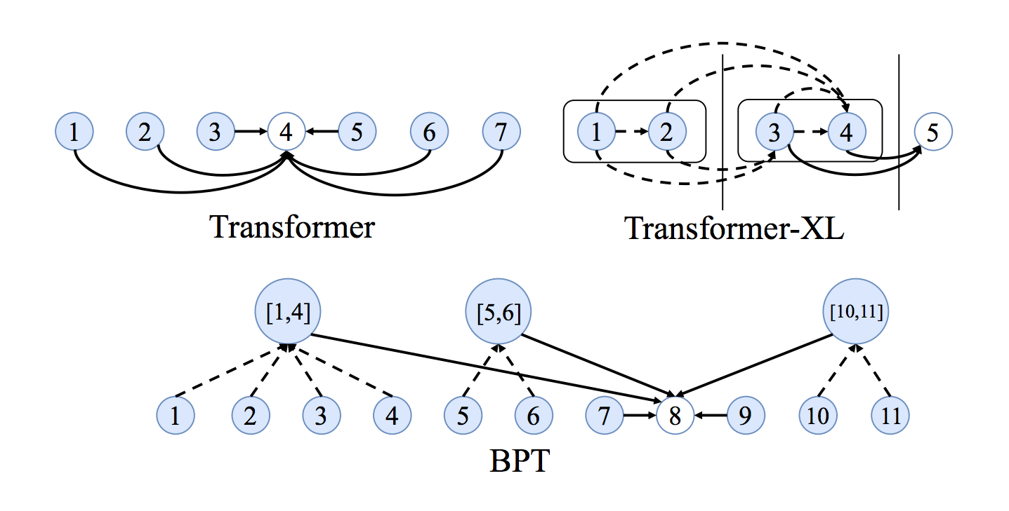
Are Transformers learning neural syntax?
- There have been several interesting papers from the NLP community on what Transformers might be learning. The basic premise is that performing attention on all word pairs in a sentence – with the purpose of identifying which pairs are the most interesting – enables Transformers to learn something like a task-specific syntax.
- Different heads in the multi-head attention might also be ‘looking’ at different syntactic properties, as shown in the figure (source) below.
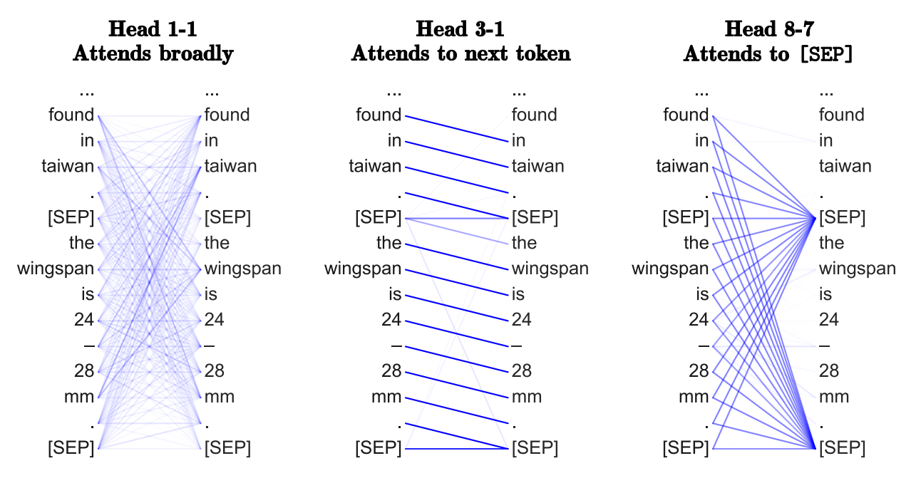
Why multiple heads of attention? Why attention?
- The optimization view of multiple attention heads is that they improve learning and help overcome bad random initializations. For instance, Analyzing Multi-Head Self-Attention: Specialized Heads Do the Heavy Lifting, the Rest Can Be Pruned and it’s accompanying post by Viota (2019) and Are Sixteen Heads Really Better than One? by Michel et al. showed that Transformer heads can be ‘pruned’ or removed after training without significant performance impact.
Benefits of Transformers compared to RNNs/GRUs/LSTMs
- The Transformer can learn longer-range dependencies than RNNs and its variants such as GRUs and LSTMs.
- The biggest benefit, however, comes from how the Transformer lends itself to parallelization. Unlike an RNN which processes a word at each time step, a key property of the Transformer is that the word at each position flows through its own path in the encoder. There are dependencies between these paths in the self-attention layer (since the self-attention layer computes how important each other word in the input sequence is to this word). However, once the self-attention output is generated, the feed-forward layer does not have those dependencies, and thus the various paths can be executed in parallel while flowing through the feed-forward layer. This is an especially useful trait in case of the Transformer encoder which can process each input word in parallel with other words after the self-attention layer. This feature, is however, not of great importance for the decoder since it generates one word at a time and thus does not utilize parallel word paths.
What would we like to fix about the transformer? / Drawbacks of Transformers
- The biggest drawback of the Transformer architecture is the quadratic computational complexity with respect to both the number of tokens (\(n\)) and the embedding size (\(d\)). This means that as sequences get longer, the time and computational resources needed for training increase significantly. A detailed discourse on this and a couple of secondary drawbacks are as below.
- Quadratic time and space complexity of the attention layer:
- Transformers use what’s known as self-attention, where each token in a sequence attends to all other tokens (including itself). This implies that the runtime of the Transformer architecture is quadratic in the length of the input sequence, which means it can be slow when processing long documents or taking characters as inputs. If you have a sequence of $$n $$ tokens, you’ll essentially have to compute attention scores for each pair of tokens, resulting in $$n^2 $$ (quadratic) computations. In other words, computing all pairs of interactions (i.e., attention over all word-pairs) during self-attention means our computation grows quadratically with the sequence length, i.e., \(O(T^2 d)\), where \(T\) is the sequence length, and \(d\) is the dimensionality.
- In a graph context, self-attention mandates that the number of edges in the graph to scale quadratically with the number of nodes, i.e., in an \(n\) word sentence, a Transformer would be doing computations over \(n^{2}\) pairs of words. Note that for recurrent models, it only grew linearly.
- This implies a large parameter count (implying high memory footprint) and thus, high computational complexity.
- Say, \(d = 1000\). So, for a single (shortish) sentence, \(T \leq 30 \Rightarrow T^{2} \leq 900 \Rightarrow T^2 d \approx 900K\). Note that in practice, we set a bound such as \(T = 512\). Imagine working on long documents with \(T \geq 10,000\)?!
- High compute requirements has a negative impact on power and battery life requirements, especially for portable device targets.
- Similarly, for storing these attention scores, you’d need space that scales with $$n^2 $$, leading to a quadratic space complexity.
- This becomes problematic for very long sequences as both the computation time and memory usage grow quickly, limiting the practical use of standard transformers for lengthy inputs.
- Overall, a transformer requires higher computational power (and thus, lower battery life) and memory footprint compared to its conventional counterparts.
- Wouldn’t it be nice for Transformers if we didn’t have to compute pair-wise interactions between each word pair in the sentence? Recent studies such as the following show that decent performance levels can be achieved without computing interactions between all word-pairs (such as by approximating pair-wise attention).
- Quadratic time complexity of linear layers w.r.t. embedding size $$d $$:
- In Transformers, after calculating the attention scores, the result is passed through linear layers, which have weights that scale with the dimension of the embeddings. If your token is represented by an embedding of size $$d $$, and if $$d $$ is greater than $$n $$ (the number of tokens), then the computation associated with these linear layers can also be demanding.
- The complexity arises because for each token, you’re doing operations in a $$d $$-dimensional space. For densely connected layers, if $$d $$ grows, the number of parameters and hence computations grows quadratically.
- Positional Sinusoidal Embedding:
- Transformers, in their original design, do not inherently understand the order of tokens (i.e., they don’t recognize sequences). To address this, positional information is added to the token embeddings.
- The original Transformer model (by Vaswani et al.) proposed using sinusoidal functions to generate these positional embeddings. This method allows models to theoretically handle sequences of any length (since sinusoids are periodic and continuous), but it might not be the most efficient or effective way to capture positional information, especially for very long sequences or specialized tasks. Hence, it’s often considered a limitation or area of improvement, leading to newer positional encoding methods like Rotary Positional Embeddings (RoPE).
- Data appetite of Transformers vs. sample-efficient architectures:
- Furthermore, compared to CNNs, the sample complexity (i.e., data appetite) of transformers is obscenely high. CNNs are still sample efficient, which makes them great candidates for low-resource tasks. This is especially true for image/video generation tasks where an exceptionally large amount of data is needed, even for CNN architectures (and thus implies that Transformer architectures would have a ridiculously high data requirement). For example, the recent CLIP architecture by Radford et al. was trained with CNN-based ResNets as vision backbones (and not a ViT-like transformer architecture).
- Put simply, while Transformers do offer accuracy lifts once their data requirement is satisfied, CNNs offer a way to deliver reasonable performance in tasks where the amount of data available is not exceptionally high. Both architectures thus have their use-cases.
Why is training Transformers so hard?
- Reading new Transformer papers makes me feel that training these models requires something akin to black magic when determining the best learning rate schedule, warmup strategy and decay settings. This could simply be because the models are so huge and the NLP tasks studied are so challenging.
- But recent results suggest that it could also be due to the specific permutation of normalization and residual connections within the architecture.
Transformers: Extrapolation engines in high-dimensional space
- The fluency of Transformers can be tracked back to extrapolation in a high dimensional space. That is what they do: capturing of high abstractions of semantic structures while learning, matching and merging those patterns on output. So any inference must be converted into a retrieval task (which then is called many names like Prompt Engineering, Chain/Tree/Graph/* of Thought, RAG, etc.), while any Transformer model is by design a giant stochastic approximation of whatever its training data it was fed.
The road ahead for Transformers
- In the field of NLP, Transformers have already established themselves as the numero uno architectural choice or the de facto standard for a plethora of NLP tasks.
- Likewise, in the field of vision, an updated version of ViT was second only to a newer approach that combines CNNs with transformers on the ImageNet image classification task at the start of 2022. CNNs without transformers, the longtime champs, barely reached the top 10!
- It is quite likely that transformers or hybrid derivatives thereof (combining concepts of self-attention with say convolutions) will be the leading architectures of choice in the near future, especially if functional metrics (such as accuracy) are the sole optimization metrics. However, along other axes such as data, computational complexity, power/battery life, and memory footprint, transformers are currently not the best choice – which the above section on What Would We Like to Fix about the Transformer? / Drawbacks of Transformers expands on.
- Could Transformers benefit from ditching attention, altogether? Yann Dauphin and collaborators’ recent work suggests an alternative ConvNet architecture. Transformers, too, might ultimately be doing something similar to ConvNets!
Choosing the right language model for your NLP use-case: key takeaways
- Some key takeaways for LLM selection and deployment:
- When evaluating potential models, be clear about where you are in your AI journey:
- In the beginning, it might be a good idea to experiment with LLMs deployed via cloud APIs.
- Once you have found product-market fit, consider hosting and maintaining your model on your side to have more control and further sharpen model performance to your application.
- To align with your downstream task, your AI team should create a short list of models based on the following criteria:
- Benchmarking results in the academic literature, with a focus on your downstream task.
- Alignment between the pre-training objective and downstream task: consider auto-encoding for NLU and autoregression for NLG. The figure below shows the best LLMs depending on the NLP use-case (image source):
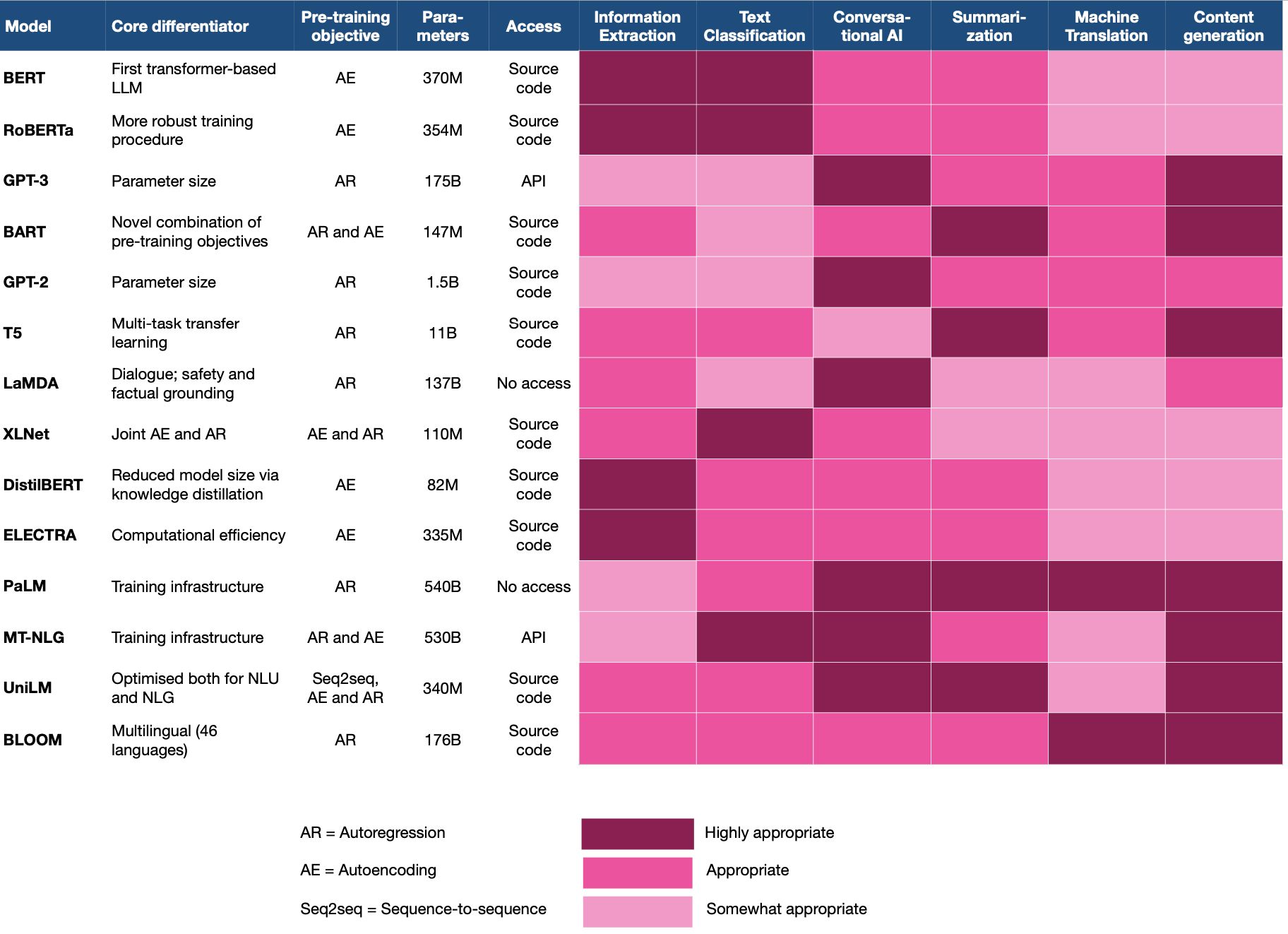
- The short-listed models should be then tested against your real-world task and dataset to get a first feeling for the performance.
- In most cases, you are likely to achieve better quality with dedicated fine-tuning. However, consider few/zero-shot learning if you don’t have the internal tech skills or budget for fine-tuning, or if you need to cover a large number of tasks.
- LLM innovations and trends are short-lived. When using language models, keep an eye on their lifecycle and the overall activity in the LLM landscape and watch out for opportunities to step up your game.
- When evaluating potential models, be clear about where you are in your AI journey:
Transformers Learning Recipe
- Transformers have accelerated the development of new techniques and models for natural language processing (NLP) tasks. While it has mostly been used for NLP tasks, it is now seeing heavy adoption in other areas such as computer vision and reinforcement learning. That makes it one of the most important modern concepts to understand and be able to apply.
- A lot of machine learning and NLP students and practitioners are keen on learning about transformers. Therefore, this recipe of resources and study materials should be helpful to help guide students interested in learning about the world of Transformers.
- To dive deep into the Transformer architecture from an NLP perspective, here’s a few links to better understand and implement transformer models from scratch.
Transformers From Scratch
-
First, try to get a very high-level introduction about transformers. Some references worth looking at:
- Transformers From Scratch (by Brandon Rohrer)
- How Transformers work in deep learning and NLP: an intuitive introduction (by AI Summer)
- Deep Learning for Language Understanding (by DeepMind)
The Illustrated Transformer
- Jay Alammar’s illustrated explanations are exceptional. Once you get that high-level understanding of transformers, going through The Illustrated Transformer is recommend for its detailed and illustrated explanation of transformers:
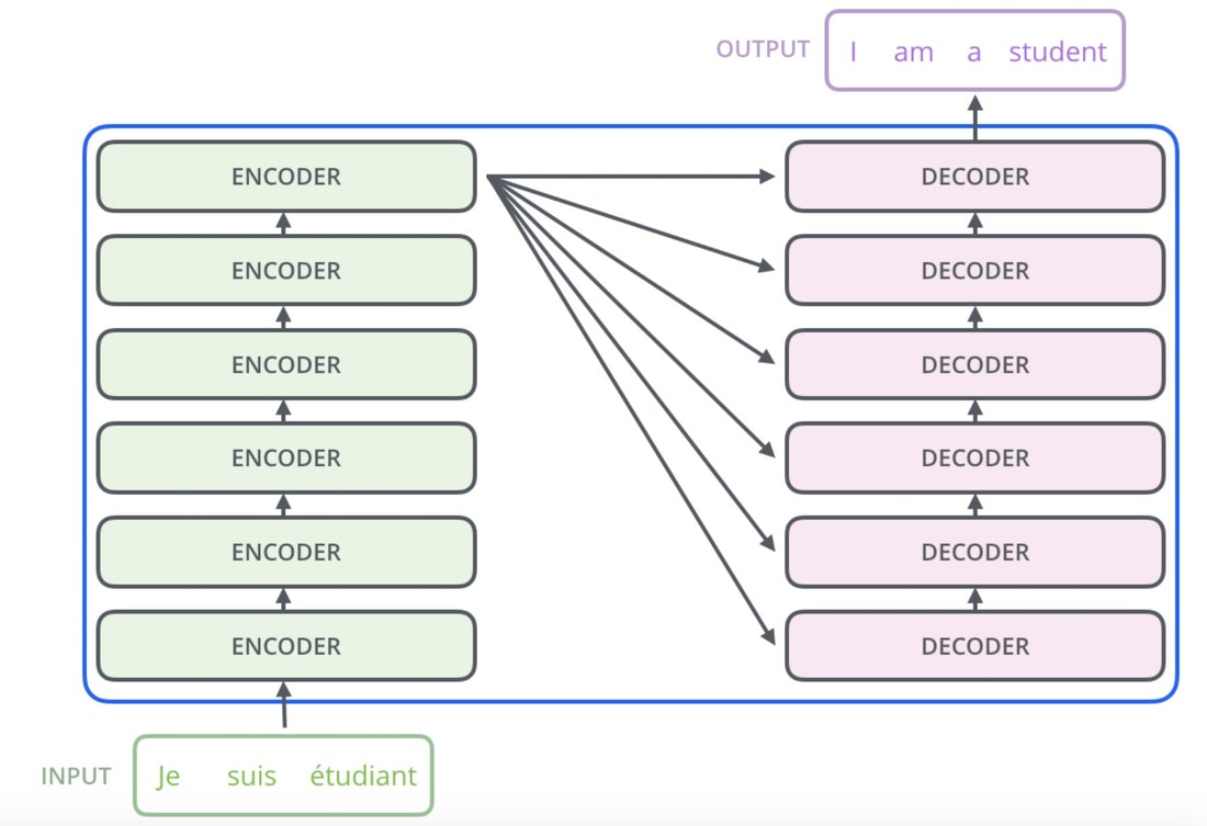
Lilian Weng’s The Transformer Family
- At this point, you may be looking for a technical summary and overview of transformers. Lilian Weng’s The Transformer Family is a gem and provides concise technical explanations/summaries:
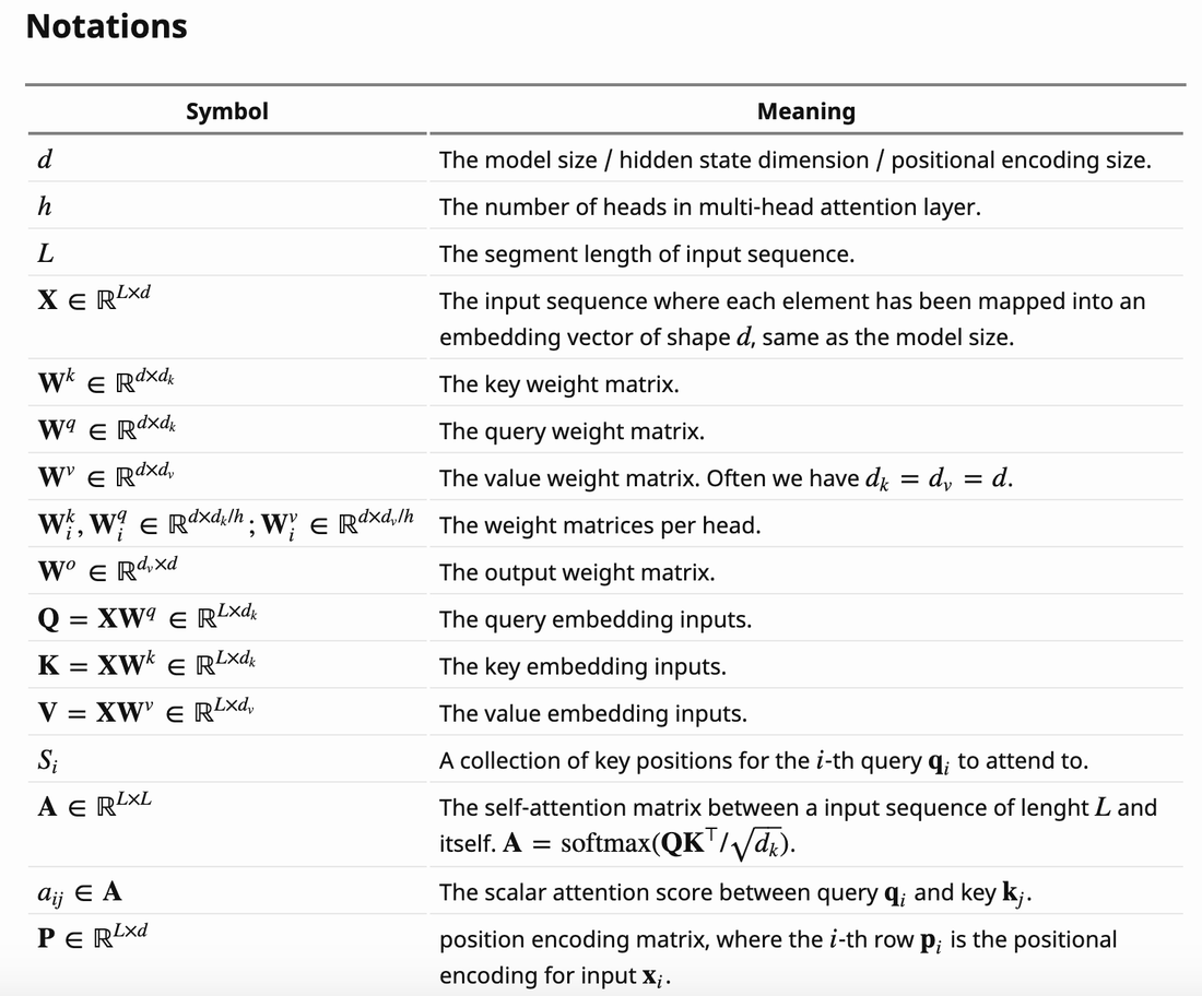
The Annotated Transformer
- Once you’ve absorbed the theory, implementing algorithms from scratch is a great way to test your knowledge and understanding of the subject matter.
- For implementing transformers in PyTorch, The Annotated Transformer offers a great tutorial. Mina Ghashami’s Transformer: Concept and Code from Scratch is also a great resource.
- For implementing transformers in TensorFlow, Transformer model for language understanding offers a great tutorial.
- Google Colab; GitHub
Attention Is All You Need
- This paper by Vaswani et al. introduced the Transformer architecture. Read it after you have a high-level understanding and want to get into the details. Pay attention to other references in the paper for diving deep.
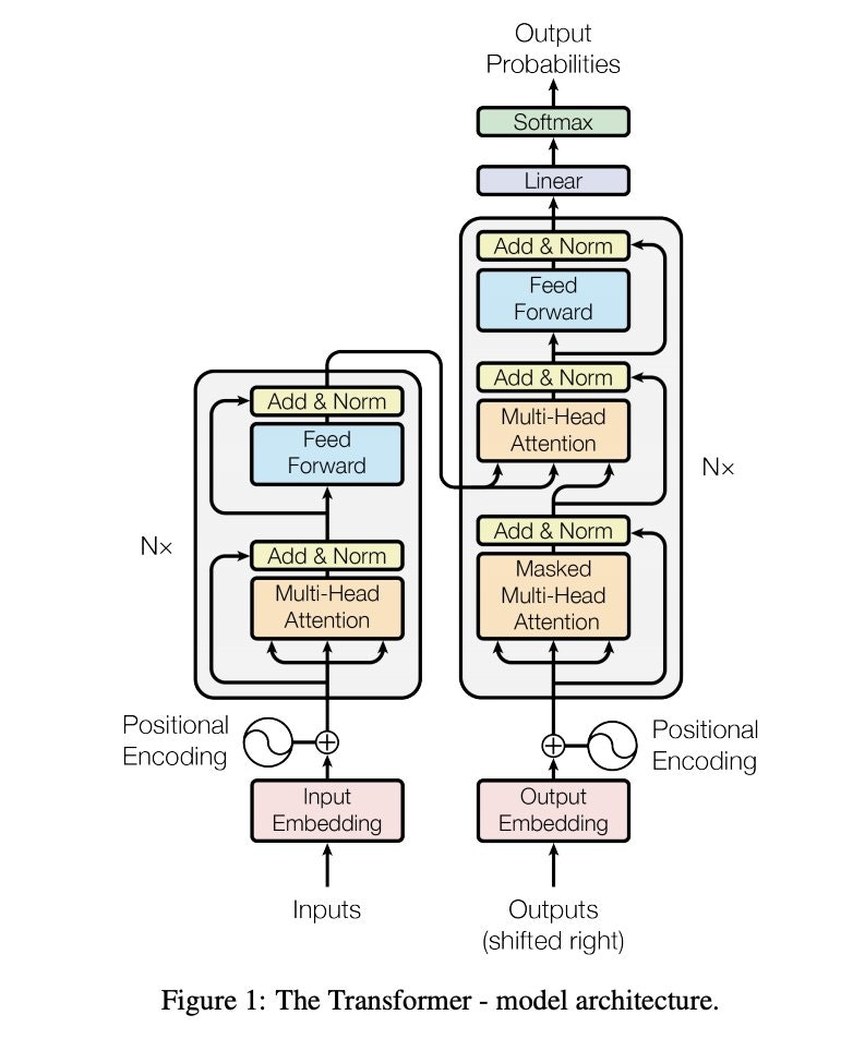
HuggingFace Encoder-Decoder Models
- With the HuggingFace Encoder-Decoder class, you no longer need to stick to pre-built encoder-decoder models like BART or T5, but can instead build your own Encoder-Decoder architecture by doing a mix-and-match with the encoder and decoder model of your choice (similar to stacking legos!), say BERT-GPT2. This is called “warm-starting” encoder-decoder models. Read more here: HuggingFace: Leveraging Pre-trained Language Model Checkpoints for Encoder-Decoder Models.
- You could build your own multimodal encoder-decoder architectures by mixing and matching encoders and decoders. For example:
- Image captioning: ViT/DEiT/BEiT + GPTx
- OCR: ViT/DEiT/BEiT + xBERT
- Image-to-Text (CLIP): ViT/DEiT/BEiT + xBERT
- Speech-to-Text: Wav2Vec2 Encoder + GPTx
- Text-to-Image (DALL-E): xBERT + DALL-E
- Text-to-Speech: xBERT + speech decoder
- Text-to-Image: xBERT + image decoder
- As an example, refer TrOCR: Transformer-based Optical Character Recognition with Pre-trained Models and Leveraging Pre-trained Checkpoints for Sequence Generation Tasks.
Transformers library by HuggingFace
- After some time studying and understanding the theory behind transformers, you may be interested in applying them to different NLP projects or research. At this time, your best bet is the Transformers library by HuggingFace.
- The Hugging Face Team has also published a new book on NLP with Transformers, so you might want to check that out as well.
Inference Arithmetic
- This blog by Kipply presents detailed few-principles reasoning about large language model inference performance, with no experiments or difficult math. The amount of understanding that can be acquired this way is really impressive and practical! A very simple model of latency for inference turns out to be a good fit for emprical results. It can enable better predictions and form better explanations about transformer inference.
Transformer Taxonomy
- This blog by Kipply is a comprehensive literature review of AI, specifically focusing on transformers. It covers 22 models, 11 architectural changes, 7 post-pre-training techniques, and 3 training techniques. The review is curated based on the author’s knowledge and includes links to the original papers for further reading. The content is presented in a loosely ordered manner based on importance and uniqueness.
GPT in 60 Lines of NumPy
- The blog post implements picoGPT and flexes some of the benefits of JAX: (i) trivial to port Numpy using
jax.numpy, (ii) get gradients, and (iii) batch withjax.vmap. It also inferences GPT-2 checkpoints.
x-transformers
- This Github repo offers a concise but fully-featured transformer, complete with a set of promising experimental features from various papers.
![]()
Speeding up the GPT - KV cache
- The blog post discusses an optimization technique for speeding up transformer model inference using Key-Value (KV) caching, highlighting its implementation in GPT models to reduce computational complexity from quadratic to linear by caching inputs for the attention block, thereby enhancing prediction speed without compromising output quality.

Transformer Poster
- A poster by Hendrik Erz that goes over how the Transformer works.
![]()
FAQs
In Transformers, how does categorical cross entropy loss enable next token prediction?
-
Core definition:
- Cross-entropy loss is a function used to measure how well a probabilistic model’s predicted distribution matches the true (target/ground truth) distribution of the data, by quantifying the “distance” between two probability distributions. It is especially common in classification problems.
-
Mathematical formulation:
- Let \(p(x)\) be the true distribution and \(q(x)\) the predicted distribution.
-
The cross-entropy from \(p\) to \(q\) is:
\[H(p, q) = - \sum_x p(x) \log q(x)\]
-
Use in classification:
-
True distribution: In classification, the true distribution is usually a one-hot distribution. For a single example with true class \(y\):
\[p(y)=1,\quad p(x\neq y)=0\] -
Predicted distribution: The model outputs class probabilities, typically via softmax, so \(q(x)\in[0,1]\) and \(\sum_x q(x)=1\).
-
With a one-hot target, the cross-entropy simplifies to the negative log-likelihood assigned to the true class under the model’s predicted distribution, and this equivalence is why cross-entropy loss is commonly referred to as the negative log-likelihood in classification settings. Mathematically, this case can be expressed as:
- Since \(H(p)\) is fixed with respect to the model, minimizing cross-entropy is equivalent to minimizing the Kullback–Leibler divergence between the true and predicted distributions.
-
-
Interpretation:
- Cross-entropy measures how many extra bits are needed to encode samples from \(p\) using a code optimized for \(q\).
- Lower cross-entropy means the predicted distribution is closer to the true one.
-
Relation to KL divergence:
-
Cross-entropy can be decomposed as:
\[H(p, q) = H(p) + \mathrm{KL}(p \Vert q)\] -
Since \(H(p)\) is fixed with respect to the model, minimizing cross-entropy is equivalent to minimizing the Kullback–Leibler divergence between the true and predicted distributions.
-
-
Key takeaway:
- Cross-entropy loss fundamentally operates on two probability distributions, even though one of them is often a one-hot in standard supervised learning.
In the transformer’s language modeling head, after the softmax function, argmax is performed which is non-differentiable. How does backprop work in this case during training?
-
During training, backprop works because argmax is not part of the computation graph; instead, gradients flow through softmax and cross-entropy, which are fully differentiable. Specifics below:
- What the model actually outputs during training:
- A transformer language model produces a vector of logits \(z \in \mathbb{R}^V\), where \(V\) is the vocabulary size and \(z_i\) is the unnormalized score for token \(i\). These logits are passed through the softmax function to obtain a probability distribution over the vocabulary:
- At this stage, the model outputs a continuous probability distribution. No discrete decision (such as argmax) is made during training.
- How the loss is computed:
- Let \(y\) denote the index of the correct (target) token. Training uses the categorical cross-entropy loss, equivalently the negative log-likelihood of the correct token under the predicted distribution:
- Substituting the softmax expression for \(p_y\) makes the dependence on the logits explicit:
- This rewritten form is crucial: the first term depends only on the correct logit \(z_y\), while the second term depends on all logits through the log-sum-exp.
- Backpropagation through softmax + cross-entropy:
- The gradient of the loss with respect to an arbitrary logit \(z_i\) is:
-
This result comes directly from differentiating the expanded loss \(\mathcal{L} = -z_y + \log \sum_j e^{z_j}\). The derivative of \(-z_y\) contributes \(-1\) when \(i = y\) and \(0\) otherwise, while the derivative of the log-sum-exp term yields \(\frac{e^{z_i}}{\sum_j e^{z_j}} = p_i\). Together, these give a simple and fully differentiable learning signal: the correct token’s logit is pushed upward, and every other logit is pushed downward in proportion to how much probability mass it currently receives.
-
This gradient is what flows backward through the language modeling head and into all preceding transformer layers.
- Where argmax actually appears:
- Argmax is only used at inference time to convert the learned probability distribution into a concrete token prediction:
- Because argmax is non-differentiable, it is intentionally excluded from training. By the time argmax is applied, gradients are no longer needed.
- Intuition:
- Training teaches the model to assign high probability to the correct token, not to “pick” a token. The discrete decision (argmax or sampling) is deferred until after training, when gradients are no longer needed.
- Why this works:
- Training does not teach the model to make a hard decision; it teaches the model to shape its probability distribution so that the correct token dominates. If \(p_y\) is close to 1 and all other probabilities are close to 0, the argmax decision at inference becomes trivial.
- Related edge cases:
- When discrete decisions must occur inside training itself (for example, in reinforcement learning, hard attention, or discrete latent variables), special techniques such as policy gradients, Gumbel-Softmax relaxations, or straight-through estimators are required. Standard transformer language model training avoids this entirely.
- What the model actually outputs during training:
Explain attention scores vs. attention weights? How are attention weights derived from attention scores?
-
Attention Scores:
- These are the raw compatibility values computed between a query \(Q\) and each key \(K\).
-
Mathematically, for a query vector \(q\) and key vectors \(K = [k_1, k_2, \dots, k_n]\), the attention scores are:
\[\text{scores}_i = \frac{q \cdot k_i}{\sqrt{d_k}}\]- where \(d_k\) is the dimension of the key vectors (used for scaling).
- These scores measure how relevant each key (and therefore its corresponding value) is to the current query.
- They can be positive or negative, large or small, and are not normalized.
- The scores reflect raw similarity or affinity before any probabilistic interpretation.
-
Attention Weights:
- After obtaining the scores, they are passed through a softmax function to convert them into a probability distribution:
- The weights are normalized (sum to 1).
- They represent the relative importance of each key (and its associated value) for the given query.
- These are the values actually used to compute the weighted average of the value vectors:
-
Intuitive Difference:
- Scores: “How much should I pay attention to this token?” (raw similarity)
-
Weights: “How much will I actually pay attention?” (normalized influence)
- Think of the softmax as turning raw attention preferences (scores) into actual attention probabilities (weights).
-
Example:
-
Suppose you have three attention scores for a query: \([2.0, 1.0, 0.1]\).
-
After applying softmax:
- So the model will focus 62% on the first token, 23% on the second, and 15% on the third — even though the raw scores were unbounded.
-
-
Tabular Comparison:
| Concept | Formula | Normalized? | Used for? |
|---|---|---|---|
| Attention scores | \(\frac{q \cdot k_i}{\sqrt{d_k}}\) | No | Similarity measure |
| Attention weights | \(\text{softmax}(\text{scores})\) | Yes (sum = 1) | Weighted combination of values |
Did the original Transformer use absolute or relative positional encoding?
- The original Transformer model, as introduced by Vaswani et al. in their 2017 paper “Attention Is All You Need”, used absolute positional encoding. This design was a key feature to incorporate the notion of sequence order into the model’s architecture.
- Absolute Positional Encoding in the Original Transformer
- Mechanism:
- The Transformer model does not inherently capture the sequential order of the input data in its self-attention mechanism. To address this, the authors introduced absolute positional encoding.
- Each position in the sequence was assigned a unique positional encoding vector, which was added to the input embeddings before they were fed into the attention layers.
- Implementation: The positional encodings used were fixed (not learned) and were based on sine and cosine functions of different frequencies. This choice was intended to allow the model to easily learn to attend by relative positions since for any fixed offset \(k, PE_{pos + k}\) could be represented as a linear function of \(PE_{pos}\).
- Mechanism:
- Importance: This approach to positional encoding was crucial for enabling the model to understand the order of tokens in a sequence, a fundamental aspect of processing sequential data like text.
- Relative and Rotary Positional Encoding in Later Models
- After the introduction of the original Transformer, subsequent research explored alternative ways to incorporate positional information. One such development was the use of relative positional encoding, which, instead of assigning a unique encoding to each absolute position, encodes the relative positions of tokens with respect to each other. This method has been found to be effective in certain contexts and has been adopted in various Transformer-based models developed after the original Transformer. Rotary positional encoding methods (such as RoPE) were also presented after relative positional encoding methods.
- Takeaways: In summary, the original Transformer model utilized absolute positional encoding to integrate sequence order into its architecture. This approach was foundational in the development of Transformer models, while later variations and improvements, including relative positional encoding, have been explored in subsequent research to further enhance the model’s capabilities.
How does the choice of positional encoding method can influence the number of parameters added to the model? Consider absolute, relative, and rotary positional encoding mechanisms.
- In Large Language Models (LLMs), the choice of positional encoding method can influence the number of parameters added to the model. Let’s compare absolute, relative, and rotary (RoPE) positional encoding in this context:
- Absolute Positional Encoding:
- Parameter Addition:
- Absolute positional encodings typically add a fixed number of parameters to the model, depending on the maximum sequence length the model can handle.
- Each position in the sequence has a unique positional encoding vector. If the maximum sequence length is \(N\) and the model dimension is \(D\), the total number of added parameters for absolute positional encoding is \(N \times D\).
- Fixed and Non-Learnable: In many implementations (like the original Transformer), these positional encodings are fixed (based on sine and cosine functions) and not learnable, meaning they don’t add to the total count of trainable parameters.
- Parameter Addition:
- Relative Positional Encoding:
- Parameter Addition:
- Relative positional encoding often adds fewer parameters than absolute encoding, as it typically uses a set of parameters that represent relative positions rather than unique encodings for each absolute position.
- The exact number of added parameters can vary based on the implementation but is generally smaller than the \(N \times D\) parameters required for absolute encoding.
- Learnable or Fixed: Depending on the model, relative positional encodings can be either learnable or fixed, which would affect whether they contribute to the model’s total trainable parameters.
- Parameter Addition:
- Rotary Positional Encoding (RoPE):
- Parameter Addition:
- RoPE does not add any additional learnable parameters to the model. It integrates positional information through a rotation operation applied to the query and key vectors in the self-attention mechanism.
- The rotation is based on the position but is calculated using fixed, non-learnable trigonometric functions, similar to absolute positional encoding.
- Efficiency: The major advantage of RoPE is its efficiency in terms of parameter count. It enables the model to capture relative positional information without increasing the number of trainable parameters.
- Parameter Addition:
- Summary:
- Absolute Positional Encoding: Adds \(N \times D\) parameters, usually fixed and non-learnable.
- Relative Positional Encoding: Adds fewer parameters than absolute encoding, can be learnable, but the exact count varies with implementation.
- Rotary Positional Encoding (RoPE): Adds no additional learnable parameters, efficiently integrating positional information.
- In terms of parameter efficiency, RoPE stands out as it enriches the model with positional awareness without increasing the trainable parameter count, a significant advantage in the context of LLMs where managing the scale of parameters is crucial.
In Transformer-based models, how does RoPE enable context length extension?
- RoPE, or Rotary Positional Embedding, is a technique used in some language models, particularly Transformers, for handling positional information. The need for RoPE or similar techniques becomes apparent when dealing with long context lengths in LLMs.
- Context Length Extension in LLMs
- Positional Encoding in Transformers:
- Traditional Transformer models use positional encodings to add information about the position of tokens in a sequence. This is crucial because the self-attention mechanism is, by default, permutation-invariant (i.e., it doesn’t consider the order of tokens).
- In standard implementations like the original Transformer, positional encodings are added to the token embeddings and are typically fixed (not learned) and based on sine and cosine functions of different frequencies.
- Challenges with Long Sequences: As the context length (number of tokens in a sequence) increases, maintaining effective positional information becomes challenging. This is especially true for fixed positional encodings, which may not scale well or capture relative positions effectively in very long sequences.
- Role and Advantages of RoPE
- Rotary Positional Embedding: RoPE is designed to provide rotational equivariance to self-attention. It essentially encodes the absolute position and then rotates the positional encoding of keys and queries differently based on their position. This allows the model to implicitly capture relative positional information through the self-attention mechanism.
- Effectiveness in Long Contexts: RoPE scales effectively with sequence length, making it suitable for LLMs that need to handle long contexts or documents. This is particularly important in tasks like document summarization or question-answering over long passages.
- Preserving Relative Positional Information: RoPE allows the model to understand the relative positioning of tokens effectively, which is crucial in understanding the structure and meaning of sentences, especially in languages with less rigid syntax.
- Computational Efficiency: Compared to other methods of handling positional information in long sequences, RoPE can be more computationally efficient, as it doesn’t significantly increase the model’s complexity or the number of parameters.
- Takeaways: In summary, RoPE is required for effectively extending the context length in LLMs due to its ability to handle long sequences while preserving crucial relative positional information. It offers a scalable and computationally efficient solution to one of the challenges posed by the self-attention mechanism in Transformers, particularly in scenarios where understanding the order and relationship of tokens in long sequences is essential.
Why is the Transformer Architecture not as susceptible to vanishing gradients compared to RNNs?
- The Transformer architecture is less susceptible to vanishing gradients compared to Recurrent Neural Networks (RNNs) due to several key differences in their design and operation:
- Self-Attention Mechanism and Parallel Processing:
- Transformers: Transformers use self-attention mechanism which allow them to directly access any position in the input sequence without the need for sequential processing. This means that the gradients can flow more easily across the entire network since there are direct connections between all input and output positions. Additionally, the self-attention mechanism and feed-forward layers in Transformers allow for parallel processing of the entire sequence, facilitating better gradient flow and more efficient training. To handle the sequential nature of data, Transformers use positional encodings added to the input embeddings, enabling them to maintain the order of the sequence while still allowing parallel processing.
- RNNs: RNNs process input sequences sequentially, step by step. This sequential processing can cause gradients to either vanish or explode as they are propagated back through many time steps during training, especially in long sequences. RNNs are typically trained using Backpropagation Through Time (BPTT), a method that unrolls the network through time and applies backpropagation. BPTT can suffer from vanishing and exploding gradients because the gradients must be propagated back through many time steps, leading to instability and difficulty in training long sequences.
- Residual Connections:
- Transformers: Each layer in a Transformer includes residual (skip) connections, which add the input of a layer to its output. These connections help gradients flow through the network more directly, mitigating the vanishing gradient problem.
- RNNs: Although some RNN architectures can incorporate residual connections, it is less common and less effective due to the inherently sequential nature of RNNs.
- Layer Normalization:
- Transformers: Transformers use layer normalization, which helps stabilize the training process and maintain gradient magnitudes.
- RNNs: While batch normalization and layer normalization can be applied to RNNs, it is more challenging and less common compared to the straightforward application in Transformers.
- Self-Attention Mechanism and Parallel Processing:
- In summary, the Transformer architecture’s reliance on parallel processing nature of self-attention (and thus the avoidance of BPTT that RNNs depend on), residual connections, and layer normalization contributes to its robustness against vanishing gradients, making it more efficient and effective for handling long sequences compared to RNNs.
What is the fraction of attention weights relative to feed-forward weights in common LLMs?
GPT
- In GPT-1 and similar transformer-based models, the distribution of parameters between attention mechanism and feed-forward networks (FFNs) is key to understanding their architecture and design. Let’s delve into the parameter allocation in GPT-1:
Model Configuration
-
GPT-1, like many models in the GPT series, follows the transformer architecture described in the original “Attention is All You Need” paper. Here’s a breakdown:
- Model Dimension (\(d_{\text{model}}\)): For GPT-1, \(d_{\text{model}}\) is typically smaller compared to later models like GPT-3. The size used in GPT-1 is 768.
- Feed-Forward Dimension (\(d_{\text{ff}}\)): The dimension of the feed-forward layers in GPT-1 is typically about 4 times the model dimension, similar to other transformers. This results in \(d_{\text{ff}} = 3072\) for GPT-1.
Attention and Feed-Forward Weights Calculation
-
Let’s calculate the typical number of parameters for each component:
- Attention Parameters:
- Query, Key, Value (QKV) Weights: Each transformer layer in GPT-1 includes multi-head self-attention with separate weights for queries, keys, and values. Each of these matrices is of size \(d_{\text{model}} \times \frac{d_{\text{model}}}{h}\), and for simplicity, the total size for Q, K, and V combined for all heads is \(d_{\text{model}} \times d_{\text{model}}\).
- Output Projection: This is another matrix of size \(d_{\text{model}} \times d_{\text{model}}\).
- Feed-Forward Network (FFN) Parameters:
- Layer Projections: Consisting of two linear transformations:
- First layer projects from \(d_{\text{model}}\) to \(d_{\text{ff}}\),
- Second layer projects back from \(d_{\text{ff}}\) to \(d_{\text{model}}\).
- Layer Projections: Consisting of two linear transformations:
Example Calculation with GPT-1 Values
- Total Attention Weights Per Layer:
- Total for Q, K, and V combined: \(768 \times 768 \times 3 = 1769472\).
- Output projection: \(768 \times 768 = 589824\).
- Total attention weights: \(1769472 + 589824 = 2359296\) parameters.
- Total Feed-Forward Weights Per Layer:
- Up-projection: \(768 \times 3072 = 2359296\),
- Down-projection: \(3072 \times 768 = 2359296\),
- Total FFN weights: \(2359296 + 2359296 = 4718592\) parameters.
Fraction of Attention to FFN Weights
- The fraction of attention weights relative to FFN weights can be calculated as:
Takeaways
- In GPT-1, the feed-forward networks hold about twice as many parameters as the attention mechanism, a typical distribution for transformer models. This emphasizes the substantial role of the FFNs in enhancing the model’s ability to process and transform information, complementing the capabilities provided by the attention mechanism. This balance is crucial for the overall performance and flexibility of the model in handling various language processing tasks.
GPT-2
- In common large language models like GPT-2, the fraction of attention weights relative to feed-forward (MLP) weights generally follows a consistent pattern due to the architecture of the transformer layers used in these models. Typically, the Multi-Layer Perceptron (MLP) blocks contain significantly more parameters than the attention blocks.
- Here’s a breakdown for better understanding:
Transformer Layer Composition
- Attention Mechanism: Each layer in a transformer-based model like GPT-2 includes multi-head self-attention mechanism. The parameters in these mechanisms consist of query, key, value, and output projection matrices.
- Feed-Forward Network (MLP): Following the attention mechanism, each layer includes an MLP block, typically consisting of two linear transformations with a ReLU activation in between.
Parameter Distribution
- Attention Weights: For each attention head, the parameters are distributed across the matrices for queries, keys, values, and the output projection. If the model dimension is \(d_{\text{model}}\) and there are \(h\) heads, each head might use matrices of size \(\frac{d_{\text{model}}}{h} \times d_{\text{model}}\) for each of the query, key, and value, and \(d_{\text{model}} \times d_{\text{model}}\) for the output projection.
- MLP Weights: The MLP usually consists of two layers. The first layer projects from \(d_{\text{model}}\) to \(d_{\text{ff}}\) (where \(d_{\text{ff}}\) is typically 4 times \(d_{\text{model}}\)), and the second layer projects back from \(d_{\text{ff}}\) to \(d_{\text{model}}\). Thus, the MLP contains weights of size \(d_{\text{model}} \times d_{\text{ff}}\) and \(d_{\text{ff}} \times d_{\text{model}}\).
Example Calculation
- For GPT-2, if we assume \(d_{\text{model}} = 768\) and \(d_{\text{ff}} = 3072\) (which is common in models like GPT-2), and the number of heads \(h = 12\):
- Attention Parameters per Layer: Each set of Q/K/V matrices is \(\frac{768}{12} \times 768 = 49152\) parameters, and there are 3 sets per head, plus another \(768 \times 768\) for the output projection, totaling \(3 \times 49152 + 589824 = 737280\) parameters for all attention heads combined per layer.
- MLP Parameters per Layer: \(768 \times 3072 + 3072 \times 768 = 4718592\) parameters.
Fraction of Attention to MLP Weights
-
Fraction: Given these typical values, the attention parameters are about 737280, and the MLP parameters are about 4718592 per layer. This gives a fraction of attention to MLP weights of roughly \(\frac{737280}{4718592} \approx 0.156\), or about 15.6%.
-
This fraction indicates that the feed-forward layers in models like GPT-2 hold a substantially larger portion of the parameters compared to the attention mechanism, emphasizing the role of the MLP in transforming representations within the network. This distribution has implications for deciding which components to adapt or optimize during tasks like fine-tuning, as the MLP layers may offer a larger scope for modification due to their greater parameter count.
BERT
- In the architecture of BERT (Bidirectional Encoder Representations from Transformers), which utilizes the transformer model structure similar to models in the GPT series, the distribution of parameters between attention mechanism and feed-forward networks (FFNs) reflects a balance that is integral to the model’s ability to perform its intended tasks. Here’s an overview of how these weights are typically distributed in BERT and similar models:
Model Configuration
- Model Dimension (\(d_{\text{model}}\)): This is the size of the hidden layers throughout the model. For example, BERT-Base uses \(d_{\text{model}} = 768\).
- Feed-Forward Dimension (\(d_{\text{ff}}\)): The dimension of the feed-forward layer is usually set to about 4 times \(d_{\text{model}}\). For BERT-Base, \(d_{\text{ff}} = 3072\).
Attention and Feed-Forward Weights Calculation
- Attention Parameters:
- Query, Key, Value (QKV) Weights: Each transformer layer in BERT has multi-head self-attention with separate weights for queries, keys, and values. For each head:
- Size of each matrix (Q, K, V): \(d_{\text{model}} \times \frac{d_{\text{model}}}{h}\), where \(h\) is the number of heads. The total size per matrix type for all heads combined is \(d_{\text{model}} \times d_{\text{model}}\).
- Output Projection Weights: Another matrix of size \(d_{\text{model}} \times d_{\text{model}}\).
- Query, Key, Value (QKV) Weights: Each transformer layer in BERT has multi-head self-attention with separate weights for queries, keys, and values. For each head:
- Feed-Forward Network (FFN) Parameters:
- Layer Projections: There are two linear transformations in the FFN block:
- The first layer projects from \(d_{\text{model}}\) to \(d_{\text{ff}}\),
- The second layer projects back from \(d_{\text{ff}}\) to \(d_{\text{model}}\).
- Layer Projections: There are two linear transformations in the FFN block:
Example Calculation with Typical Values
- Attention Weights Per Layer:
- For Q, K, and V: \(768 \times 768 \times 3 = 1769472\) (each type has size \(768 \times 768\)).
- Output projection: \(768 \times 768 = 589824\).
- Total Attention Weights: \(1769472 + 589824 = 2359296\) parameters.
- Feed-Forward Weights Per Layer:
- Up-projection: \(768 \times 3072 = 2359296\),
- Down-projection: \(3072 \times 768 = 2359296\),
- Total FFN Weights: \(2359296 + 2359296 = 4718592\) parameters.
Fraction of Attention to FFN Weights
- The fraction of attention weights relative to FFN weights can be calculated as:
Takeaways
- In BERT, like in many transformer models, the feed-forward networks hold about twice as many parameters as the attention mechanism. This indicates a strong emphasis on the transformation capabilities of the FFNs, crucial for enabling BERT to generate context-rich embeddings for various NLP tasks. The FFN layers in BERT and similar models play a pivotal role in enhancing the model’s representational power, ensuring it can handle complex dependencies and nuances in language understanding and generation tasks.
In BERT, how do we go from \(Q\), \(K\), and \(V\) at the final transformer block’s output to contextualized embeddings?
- To understand how the \(Q\), \(K\), and \(V\) matrices contribute to the contextualized embeddings in BERT, let’s dive into the core processes occurring in the final layer of BERT’s transformer encoder stack. Each layer performs self-attention, where the matrices \(Q\), \(K\), and \(V\) interact to determine how each token attends to others in the sequence. Through this mechanism, each token’s embedding is iteratively refined across multiple layers, progressively capturing both its own attributes and its contextual relationships with other tokens.
- By the time these computations reach the final layer, the output embeddings for each token are highly contextualized. Each token’s embedding now encapsulates not only its individual meaning but also the influence of surrounding tokens, providing a rich representation of the token in context. This final, refined embedding is what BERT ultimately uses to represent each token, balancing individual token characteristics with the nuanced context in which the token appears.
-
Let’s dive deeper into how the \(Q\), \(K\), and \(V\) matrices at each layer ultimately yield embeddings that are contextualized, particularly by looking at what happens in the final layer of BERT’s transformer encoder stack. The core steps involved from self-attention outputs in the last layer to meaningful embeddings per token are:
-
Self-Attention Mechanism Recap:
- In each layer, BERT computes self-attention across the sequence of tokens. For each token, it generates a query vector \(Q\), a key vector \(K\), and a value vector \(V\). These matrices are learned transformations of the token embeddings and encode how each token should attend to other tokens.
- For each token in the sequence, self-attention calculates attention scores by comparing \(Q\) with \(K\), determining the influence or weight of other tokens relative to the current token.
-
Attention Weights Calculation:
- For each token, the model computes the similarity of its \(Q\) vector with every other token’s \(K\) vector in the sequence. This similarity score is then normalized (typically through softmax), resulting in attention weights.
- These weights tell us the degree to which each token should “attend to” (or incorporate information from) other tokens.
-
Weighted Summation of Values (Producing Contextual Embeddings):
- Using the attention weights, each token creates a weighted sum over the \(V\) vectors of other tokens. This weighted sum serves as the output of the self-attention operation for that token.
- Each token’s output is thus a combination of other tokens’ values, weighted by their attention scores. This result effectively integrates context from surrounding tokens.
-
Passing Through Multi-Head Attention and Feed-Forward Layers:
- BERT uses multi-head attention, meaning that it performs multiple attention computations (heads) in parallel with different learned transformations of \(Q\), \(K\), and \(V\).
- Each head provides a different “view” of the relationships between tokens. The outputs from all heads are concatenated and then passed through a feed-forward layer to further refine each token’s representation.
-
Stacking Layers for Deeper Contextualization:
- The output from the multi-head attention and feed-forward layer for each token is passed as input to the next layer. Each subsequent layer refines the token embeddings by adding another layer of attention-based contextualization.
- By the final layer, each token embedding has been repeatedly updated, capturing nuanced dependencies from all tokens in the sequence through multiple self-attention layers.
-
Extracting Final Token Embeddings from the Last Encoder Layer:
- After the last layer, the output matrix contains a contextualized embedding for each token in the sequence. These embeddings represent the final “meaning” of each token as understood by BERT, based on the entire input sequence.
- For a sequence with \(n\) tokens, the output from the final layer is a matrix of shape \(n \times d\), where \(d\) is the embedding dimension.
-
Embedding Interpretability and Usage:
- The embedding for each token in this final matrix is now contextualized; it reflects not just the identity of the token itself but also its role and relationships within the context of the entire sequence.
- These final embeddings can be used for downstream tasks, such as classification or question answering, where the model uses these embeddings to predict task-specific outputs.
What gets passed on from the output of the previous transformer block to the next in the encoder/decoder?
-
In a transformer-based architecture (such as the vanilla transformer or BERT), the output of each transformer block (or layer) becomes the input to the subsequent layer in the stack. Specifically, here’s what gets passed from one layer to the next:
-
Token Embeddings (Contextualized Representations):
- The main component passed between layers is a set of token embeddings, which are contextualized representations of each token in the sequence up to that layer.
- For a sequence of \(n\) tokens, if the embedding dimension is \(d\), the output of each layer is an \(n \times d\) matrix, where each row represents the embedding of a token, now updated with contextual information learned from the previous layer.
- Each embedding at this point reflects the token’s meaning as influenced by the other tokens it attended to in that layer.
-
Residual Connections:
- Transformers use residual connections to stabilize training and allow better gradient flow. Each layer’s output is combined with its input via a residual (or skip) connection.
- In practice, the output of the self-attention and feed-forward operations is added to the input embeddings from the previous layer, preserving information from the initial representation.
-
Layer Normalization:
- After the residual connection, layer normalization is applied to the summed representation. This normalization helps stabilize training by maintaining consistent scaling of token representations across layers.
- The layer-normalized output is then what gets passed on as the “input” to the next layer.
-
Positional Information:
- The positional embeddings (added initially to the token embeddings to account for the order of tokens in the sequence) remain embedded in the representations throughout the layers. No additional positional encoding is added between layers; instead, the attention mechanism itself maintains positional relationships indirectly.
-
Summary of the Process:
- Each layer receives an \(n \times d\) matrix (the sequence of token embeddings), which now includes contextual information from previous layers.
- The layer performs self-attention and passes the output through a feed-forward network.
- The residual connection adds the original input to the output of the feed-forward network.
- Layer normalization is applied to this result, and the final matrix is passed on as the input to the next layer.
- This flow ensures that each successive layer refines the contextual embeddings for each token, building progressively more sophisticated representations of tokens within the context of the entire sequence.
In the vanilla transformer, what gets passed on from the output of the encoder to the decoder?
- In the original (vanilla) Transformer model, the encoder processes the input sequence and produces a sequence of encoded representations, often referred to as “encoder output” or “memory.” This encoder output is then fed into each layer of the decoder to help it generate the target sequence.
-
Specifically:
-
What is passed from encoder to decoder:
- The encoder passes the full sequence of encoder output representations \(z = (z_1, \dots,\)z_n\()\), one vector per input position (token index, conceptually equivalent to a time step).
- Note that a position/index here refers to a token index in the input sequence, which plays the same conceptual role as a time step in RNNs. Unlike RNNs, these positions are processed in parallel rather than sequentially in time.
- This sequence acts as a fixed memory that the decoder can attend to in parallel via cross-attention at every decoding step, without compressing the sequence into a single vector (unlike classic RNN encoder–decoder models, which typically pass only a single final hidden state to the decoder).
- Note that there is no compression into a single vector; all positions are preserved and accessible.
- The encoder passes the full sequence of encoder output representations \(z = (z_1, \dots,\)z_n\()\), one vector per input position (token index, conceptually equivalent to a time step).
-
What \(z\) represents:
- Each \(z_i\) is a contextualized hidden state of dimension \(d_{\text{model}}\) corresponding to input position (time step) \(i\).
- \(z\) is computed by passing token embeddings plus positional encodings through a stack of self-attention and position-wise feed-forward layers in the encoder.
- The final encoder layer outputs are used directly, without pooling or recurrence, as keys and values for decoder cross-attention.
-
How the decoder uses the encoder output:
-
In the encoder–decoder (cross) attention sub-layer, the decoder supplies queries \(Q\), while the encoder outputs \(z\) are projected to the keys \(K\) and values \(V\):
\[Q = H^{\text{dec}} W^Q, \quad K = Z W^K, \quad V = Z W^V\]- where \(Z\) is the matrix formed by stacking \((z_1, \dots,\)z_n\()\).
-
The attention output is computed as:
\[\text{Attention}(Q, K, V) = \text{softmax} \left(\frac{Q K^\top}{\sqrt{d_k}}\right)V\] -
Each decoder position can attend to all encoder positions simultaneously, enabling flexible alignment between input and output tokens.
-
-
Key architectural implication:
- The encoder–decoder connection is realized entirely through attention, not through sequential hidden-state transfer as in RNN-based models.
-
- In summary, the encoder output \(z\) serves as the source of information for the decoder, allowing it to attend over this sequence during generation to access context from the input sequence through cross-attention in each decoder layer.
Self-attention ensures that the last token’s hidden state already encodes information from all previous tokens (subject to causal masking). If each hidden state \(z\) contains contextual information from the entire input sequence, why does the encoder still pass the full sequence of hidden states to the decoder via cross-attention? Why is it insufficient to provide only \(z_n\) corresponding to the hidden state of the last token?
Although each encoder hidden state \(z_i\) is globally contextualized through self-attention, providing only the final encoder state would significantly constrain the expressiveness of the encoder–decoder interface. The decoder depends on structured, selective access to the input sequence rather than on a single compressed summary.
-
Contextualization does not imply lossless compression
- Each encoder hidden state \(z_i\) incorporates information from all input tokens, but it remains specialized to represent token \(i\) in its local and global context.
- Collapsing the entire source sequence into a single vector \(z_n\) would force all alignment-relevant, syntactic, and semantic information into a fixed-dimensional bottleneck. This would reintroduce the core limitation of early recurrent encoder–decoder models, in which the final hidden state was required to encode the full source sequence and often failed to preserve fine-grained structure.
-
The decoder treats encoder outputs as associative memory
- In encoder–decoder Transformers, the decoder does not consume encoder representations as a single summary vector. Instead, it treats the collection of encoder hidden states as an associative, content-addressable memory.
- At each decoding step, the decoder forms a query from its current hidden state and compares it against keys derived from all encoder positions, retrieving and combining information from the most relevant source tokens. This mechanism allows the decoder to reference different aspects of the input sequence on demand, rather than relying on a fixed, precomputed summary.
-
Position-specific access is essential for alignment
- Different target tokens require information from different source positions. Early decoding steps may rely more heavily on early source tokens, while later steps may depend on distant or structurally related elements. Retaining all encoder hidden states enables the decoder to perform this token-level, position-specific alignment dynamically. A single vector \(z_n\), regardless of how much contextual information it contains, cannot support this level of flexible conditioning.
-
Self-attention distributes information without collapsing structure
- Encoder self-attention enables global information flow across the input sequence, but it deliberately preserves a set of position-indexed representations rather than collapsing them into a single state. This design avoids a sequential or final-state bottleneck and maintains a structured representation space that the decoder can query in parallel. Cross-attention then exploits this structure by allowing each decoder step to select and combine encoder states in a task-dependent manner.
-
In summary, although each encoder hidden state encodes information about the entire input, the full sequence of encoder outputs is required because the decoder treats them as an associative memory over the source. This design enables flexible, fine-grained access to input information and avoids the representational bottleneck that would arise from passing only a single encoder hidden state.
Self-attention ensures that the last token’s hidden state already encodes information from all previous tokens (subject to causal masking). As such, the hidden state at the final decoder position is used to generate the next token. Why is this the case, given that the encoder provides the decoder with the full sequence of encoder hidden states via cross-attention?
-
This behavior follows directly from the distinct roles played by self-attention and cross-attention in an autoregressive encoder–decoder Transformer, and from the causal structure of next-token prediction.
-
Self-attention with causal masking yields a complete conditional representation
- In a causally masked self-attention layer, the hidden state at decoder position n is computed using a query from position \(n\) and keys and values from all positions \(1\) through \(n\). As a result, the hidden representation at the final position is a function of the entire available target-side context. Formally, autoregressive decoding defines the next-token distribution as: \(p(y_{n+1} \mid y_1, \ldots, y_n)\).
- The hidden state at position n is the only decoder state that is conditioned on exactly the full prefix y₁ … yₙ and nothing beyond it. Earlier decoder states z_i for i < n are conditioned on strictly smaller prefixes and therefore do not encode the complete conditioning context required for predicting yₙ₊₁.
-
Only one new hidden state is computed per decode step
- During decoding, the model computes a hidden representation only for the newly added position. Self-attention at that step uses cached key–value pairs from all previous positions, allowing the current query to aggregate information from the entire history. Although attention spans all prior tokens, the output of this computation is a single vector corresponding to the current position. The output projection that produces logits for the next token is applied exclusively to this current-position hidden state.
-
Next-token prediction requires a single sufficient statistic
Autoregressive generation requires a single representation that summarizes “everything seen so far” in order to parameterize the conditional distribution of the next token. The causally masked self-attention mechanism is explicitly designed to construct such a representation at the final position. Using earlier hidden states would be insufficient because they lack information about later tokens in the prefix.
-
Why this does not contradict the role of the encoder
-
The encoder operates under different constraints and objectives. Encoder self-attention is typically bidirectional, and its goal is not to predict a next token but to produce a set of contextualized representations, one per source position. These representations preserve token-level structure so that the decoder can flexibly attend to different source positions as needed.
-
Cross-attention in the decoder therefore treats encoder outputs as an addressable memory rather than as a summary. At each decoding step, the decoder’s current hidden state queries all encoder hidden states to extract the source-side information most relevant to predicting the next target token. This process requires access to all encoder states, not a collapsed representation.
-
-
Key distinction between decoder self-attention and encoder outputs
- Decoder self-attention performs aggregation across time, collapsing target-side history into the hidden state at the current position because the task is next-token prediction. Encoder outputs remain uncollapsed because the task is alignment and conditional retrieval, where different target tokens may need to attend to different source tokens.
-
In summary, the decoder uses the hidden state at the final position to generate the next token because causal self-attention makes that state a sufficient statistic for the entire target-side prefix, while encoder–decoder attention relies on the full set of encoder states to support flexible, position-specific conditioning.
How does attention mask differ for encode vs. decoder models? How is loss masking enforced?
-
Attention Mask: Encoder Models (e.g., BERT, RoBERTa):
- Purpose: Hide padding tokens so they don’t influence the contextual representations.
- Structure: A 2D mask where
1marks real tokens and0marks padded tokens. -
Effect: During self-attention, any position corresponding to padding gets a large negative bias (typically −1e9) before the softmax, effectively setting its attention weight to zero.
- Mathematically, if \(A\) is the attention score matrix and \(M\) is the mask, the softmax is applied as:
- This ensures only valid (non-padded) tokens contribute to the attention distribution.
-
Attention Mask: Decoder Models (e.g., GPT-2, LLaMA, Mistral):
- Purpose: Prevent the model from “seeing the future” (causal masking) and optionally ignore padding (in batched settings).
-
Structure: Usually a causal lower-triangular mask, sometimes combined with a padding mask.
- Causal mask: ensures each position i can only attend to positions ≤ i.
- Padding mask: optional — used when batching sequences of different lengths.
- Formally, the effective attention mask is a combination:
- So the decoder’s attention mask enforces temporal directionality, unlike the encoder’s, which only enforces padding exclusion.
-
Attention Mask: Encoder–Decoder Models (e.g., T5, BART, MarianMT):
- Encoder mask: same as encoder-only models (mask padding).
- Decoder self-attention mask: causal, like GPT-2.
- Cross-attention mask: uses the encoder’s padding mask to prevent attending to padded encoder tokens.
-
Loss Masking:
-
During training, models compute loss over token predictions — typically cross-entropy between predicted logits and target token IDs.
-
However, padded tokens must not contribute to the loss, so a loss mask (often derived from the same
attention_mask) is applied:
-
where:
mask_i = 1for valid tokens,0for padding,- The denominator ensures loss normalization ignores padded positions.
-
In PyTorch (e.g., Hugging Face), this is typically done by setting the
ignore_indexinCrossEntropyLossto the tokenizer’spad_token_id, so the loss for padded tokens is automatically skipped.
-
-
In essence:
- The encoder’s mask filters out meaningless padding.
- The decoder’s mask both filters padding and blocks access to future tokens.
- Loss masking ensures padded positions never affect gradient updates or perplexity.
Further Reading
- The Illustrated Transformer
- The Annotated Transformer
- Transformer models: an introduction and catalog
- Deep Learning for NLP Best Practices
- What is Teacher Forcing for Recurrent Neural Networks?
- What is Teacher Forcing?
- The Transformer Family
- Transformer: Concept and Code from Scratch
- Transformer Inference Arithmetic
- Transformer Taxonomy
References
- Transformers are Graph Neural Networks
- Transformers from Scratch by Brandon Rohrer
- Transformers from Scratch by Peter Bloem
- Positional encoding tutorial by Amirhossein Kazemnejad
- What is One Hot Encoding? Why and When Do You Have to Use it?
- Wikipedia: Dot product
- Wikipedia: Byte pair encoding
- Will Transformers Take Over Artificial Intelligence?
- Transformer Recipe
- The decoder part in a transformer model
- Why encoder input doesn’t have a start token?
- What is the cost function of a transformer?
- Transformer models: an introduction and catalog
- Why does a transformer not use an activation function following the multi-head attention layer?
- CNN Explainer: Learn Convolutional Neural Network (CNN) in your browser!
- Where is dropout placed in the original transformer?
Citation
If you found our work useful, please cite it as:
@article{Chadha2020DistilledTransformers,
  title   = {Transformers},
  author  = {Chadha, Aman},
  journal = {Distilled AI},
  year    = {2020},
  note    = {\url{https://aman.ai}}
}