Primers • Skip/Residual Connections
- Overview
- The Vanishing Gradient Problem
- Skip Connections
- Residual Networks (ResNet)
- Skip Connections in the Transformer Architecture
- Pre-Norm and Post-Norm Skip Connections
- Evolution of Skip Connections and Residual Connections
- DenseNet
- U-Net and Long Skip Connections
- Motivation
- Encoder-decoder architecture
- Long skip connections
- Why concatenation instead of addition?
- Information preservation across scale
- Multi-scale feature fusion
- Comparison with other skip connections
- Strengths and limitations
- Influence on modern architectures
- Transition to modern residual architectures
- Attention Residuals
- Block Attention Residuals
- Hyper-Connections
- Manifold-Constrained Hyper-Connections
- Why unconstrained residual routing becomes unstable
- Identity mapping as signal conservation
- The mHC constraint
- The Birkhoff polytope
- Stability properties
- Parameterization and projection
- Sinkhorn-Knopp projection
- Manifold constraints beyond the residual mapping
- Systems efficiency
- Empirical behavior
- Relationship to standard residual connections
- Relationship to Attention Residuals
- Interpretation
- Transition to comparative design guidance
- Comparative Design Guidance
- Evolution of design objectives
- Comparison of skip and residual connection paradigms
- Fixed versus adaptive connectivity
- Addition versus concatenation
- Single-stream versus multi-stream architectures
- Static versus dynamic aggregation
- Optimization and systems tradeoffs
- Design guidelines
- Future directions
- References
- Foundational residual connections and identity mapping
- Skip connections in segmentation and biomedical vision
- Transformer architectures and normalization
- Attention Residuals and depth-wise aggregation
- Hyper-Connections and residual stream generalization
- Manifold-Constrained Hyper-Connections and stability
- Optimization, scaling, and efficiency
- Books, blogs, explainers, and ecosystem discussions
Overview
-
Modern deep learning architectures owe much of their success to a deceptively simple architectural innovation: the skip connection. Originally introduced as a practical solution to the vanishing gradient problem and the optimization difficulties of very deep convolutional networks, skip connections have since evolved into one of the defining organizational principles of modern neural network design. They are now ubiquitous across convolutional neural networks (CNNs), encoder-decoder architectures, graph neural networks (GNNs), diffusion models, and, perhaps most importantly, Transformer-based large language models (LLMs). Although their implementation often consists of nothing more than forwarding an intermediate representation around one or more layers and combining it later, their impact extends far beyond facilitating gradient propagation. Skip connections fundamentally change how neural networks represent, preserve, transform, retrieve, and route information across depth.
-
The introduction of skip connections marked a turning point in deep learning. Prior to their widespread adoption, increasing network depth frequently led to optimization failures rather than improved performance. While deeper networks possess greater representational capacity in principle, they proved difficult to train in practice due to unstable optimization dynamics. Early research primarily attributed this phenomenon to vanishing and exploding gradients, where repeated multiplication by layer Jacobians caused gradients to either diminish toward zero or grow without bound during backpropagation. However, subsequent work showed that these issues were only part of a broader optimization challenge. As networks became deeper, information itself became increasingly difficult to preserve across layers, forcing each successive transformation to reconstruct representations that had gradually degraded or drifted away from the original input.
-
The emergence of residual learning fundamentally changed this perspective. Rather than viewing each layer as learning a complete transformation from its input to its output, Deep Residual Learning for Image Recognition by He et al. (2015) proposed that layers instead learn residual functions relative to an identity mapping. This reformulation introduced an explicit pathway through which both information and gradients could propagate largely unchanged, dramatically simplifying optimization and enabling the successful training of networks containing hundreds and eventually thousands of layers. Shortly thereafter, Identity Mappings in Deep Residual Networks by He et al. (2016) provided a theoretical explanation for this behavior, demonstrating that preserving an exact identity path stabilizes both forward information propagation and backward gradient flow.
-
Although residual connections were originally introduced to solve an optimization problem in convolutional vision models, their significance has grown considerably over the past decade. Identity mappings enabled the successful optimization of extremely deep networks, Dense connectivity demonstrated the value of preserving intermediate representations, long skip connections showed that information can be propagated across changes in spatial scale, and modern Transformer architectures transformed residual pathways into persistent computational state. In contemporary LLMs, the residual stream serves as the primary carrier of information across depth, while attention mechanisms, feed-forward networks, mixture-of-experts layers, retrieval modules, and other architectural components operate by writing incremental updates into this shared representation. Consequently, understanding skip connections has become essential for understanding how modern language models compute.
-
This evolution reflects a broader shift in how residual connections are interpreted. Early work viewed them primarily as shortcuts that eased optimization by mitigating vanishing gradients. More recent research instead interprets residual pathways as learnable communication channels through which information propagates across network depth. Under this perspective, the central design question is no longer simply whether information should bypass intermediate transformations, but rather how information should be accumulated, routed, weighted, preserved, and transformed throughout increasingly deep architectures.
-
Recent advances illustrate this transition. Hyper-Connections by Zhu et al. (2024) generalize the traditional single residual stream into multiple interacting streams connected through learned mappings, allowing residual pathways themselves to become trainable architectural components. Building upon this idea, mHC: Manifold-Constrained Hyper-Connections by Xie et al. (2025) demonstrates that unconstrained residual mixing can destabilize optimization and proposes constraining residual transformations to the manifold of doubly stochastic matrices, preserving many of the stability properties that originally made residual connections successful. Meanwhile, Attention Residuals by Kimi Team et al. (2026) reinterpret residual accumulation itself as an attention problem, replacing fixed additive aggregation with learned depth-wise attention that allows each layer to selectively retrieve information from earlier representations. Together, these works indicate that residual connections are evolving from fixed architectural primitives into adaptive, learnable, and geometrically structured mechanisms for routing information across network depth.
-
This progression closely mirrors earlier developments in sequence modeling. Recurrent neural networks compress all previous sequence information into a single hidden state, creating bottlenecks that ultimately motivated the development of attention mechanisms. Similarly, conventional residual connections compress all previous layer outputs into a single accumulated residual stream through uniform addition. As architectures continue to scale in both parameter count and depth, this fixed accumulation strategy increasingly limits the model’s ability to selectively retrieve and combine information generated by earlier layers. Modern residual architectures therefore seek to replace static accumulation with adaptive routing, allowing models to determine dynamically which representations should be preserved, emphasized, revisited, or transformed.
-
Understanding these developments requires more than familiarity with individual architectures. Skip connections influence optimization, representational learning, numerical stability, distributed training, systems efficiency, and scaling behavior. Their implementation interacts closely with normalization layers, initialization schemes, activation functions, parallel training strategies, memory management, and inference latency. Consequently, the study of skip connections spans multiple levels of abstraction, ranging from mathematical analysis of gradient propagation to practical engineering considerations involved in training frontier-scale language models. Viewed through this broader perspective, skip connections are no longer simply shortcuts. They are the infrastructure through which modern neural networks preserve, retrieve, transform, and route information across increasingly deep and complex computational graphs.
-
This primer traces that evolution from first principles. It begins with the mathematical foundations of backpropagation and the optimization challenges encountered in deep neural networks before introducing skip connections as a solution to these problems. It then examines the emergence of residual learning, identity mappings, DenseNet-style feature reuse, and skip connections in encoder-decoder architectures. Building upon these foundations, the primer explores how residual pathways were adapted to Transformer architectures, including the transition from Post-Norm to Pre-Norm formulations and the resulting residual stream abstraction that underpins modern LLMs. Finally, it examines recent advances that generalize residual connections beyond fixed identity mappings, including Hyper-Connections, Manifold-Constrained Hyper-Connections, and Attention Residuals, highlighting how these architectures reinterpret residual pathways as adaptive mechanisms for information routing across depth.
-
Rather than treating these developments as isolated architectural innovations, this primer presents them as successive stages in the evolution of a common underlying principle: preserving useful information while enabling increasingly expressive transformations. From the identity shortcuts introduced in ResNet to the depth-wise attention mechanisms proposed in Attention Residuals, each advancement seeks to balance representational flexibility with stable optimization. Viewed collectively, they illustrate how a seemingly simple architectural modification reshaped an entire field and evolved into one of the defining organizational principles of modern deep learning. Their continued evolution reflects a broader shift in neural network design, from viewing layers as isolated computational units toward viewing entire architectures as structured systems for information flow.
Why skip connections matter
-
Skip connections address a fundamental tension in deep learning. Increasing depth generally increases a network’s representational capacity, allowing it to model progressively more complex hierarchical abstractions. However, greater depth also lengthens the computational graph through which both information and gradients must propagate, making optimization substantially more difficult. Skip connections alleviate this tension by introducing alternative pathways that shorten the effective distance over which signals must travel, enabling deeper networks without sacrificing trainability.
-
Beyond optimization, skip connections encourage feature reuse and information preservation. Earlier representations often contain fine-grained information that later layers would otherwise need to reconstruct. Rather than repeatedly relearning these features, skip connections allow them to remain directly accessible throughout the network. This principle appears in multiple architectural forms, including additive residual learning in ResNet, concatenative feature reuse in DenseNet, long-range encoder-decoder skip connections in U-Net, and persistent residual streams in Transformers.
Historical context
-
The idea of bypassing intermediate computation predates ResNet. Learning Representations by Back-Propagating Errors by Rumelhart et al. (1986) established the backpropagation algorithm that made deep learning feasible, but optimization remained challenging as networks grew deeper. Highway Networks by Srivastava et al. (2015) introduced gated skip pathways inspired by recurrent neural networks, allowing information to flow around nonlinear transformations through learned gates. Shortly thereafter, ResNet simplified this concept by replacing learned gates with fixed identity mappings, demonstrating that this simpler formulation was sufficient to enable unprecedented network depths while improving both optimization and generalization.
-
Subsequent architectures extended the idea in different directions. DenseNet emphasized explicit feature reuse through concatenative connections, U-Net demonstrated the importance of long-range skip connections in encoder-decoder models, and Transformer architectures adapted residual learning to sequential modeling. Today, residual pathways form the computational backbone of nearly every frontier language model, and newer designs reinterpret them as adaptive communication mechanisms rather than passive shortcuts.
Skip connections as an architectural primitive
- Modern architectures increasingly treat skip connections not as auxiliary optimization mechanisms but as primary computational structures. In Transformers, residual streams provide persistent state that every layer reads from and writes to. Hyper-Connections reinterpret residual pathways as learnable routing networks spanning multiple streams, while Attention Residuals replace uniform accumulation with adaptive retrieval across depth. These developments suggest that future neural architectures may devote as much design effort to information routing as to individual layer transformations.
Scope of this primer
-
This primer examines skip connections from both theoretical and practical perspectives. It begins with the mathematical foundations of optimization before progressively introducing increasingly sophisticated residual architectures. Along the way, it connects classical convolutional networks with modern Transformer-based language models, highlighting the common principles that underlie seemingly disparate architectures.
-
The following sections therefore move from the fundamentals of backpropagation and gradient propagation to contemporary research on adaptive residual routing, providing both the historical context and mathematical intuition necessary to understand why skip connections remain one of the most influential ideas in deep learning.
Prelude: Backpropagation
-
Before understanding why skip connections revolutionized deep learning, it is important to first understand how neural networks are trained. Nearly every architectural innovation discussed throughout this primer, from ResNet and DenseNet to Transformer residual streams, Attention Residuals, and Manifold-Constrained Hyper-Connections, ultimately exists to improve optimization. These architectures do not change the objective being optimized; rather, they change how efficiently information and gradients propagate through increasingly deep computational graphs.
-
Backpropagation is the algorithm that enables this optimization. Introduced in Learning Representations by Back-Propagating Errors by Rumelhart et al. (1986), it provides an efficient procedure for computing gradients of a scalar loss function with respect to every learnable parameter in a neural network. Rather than computing each derivative independently, which would be computationally infeasible for modern models containing billions of parameters, backpropagation systematically applies the chain rule in reverse order through the computational graph. This allows all gradients to be computed in time proportional to the cost of a single forward evaluation.
-
Although often presented as a training algorithm in its own right, backpropagation is more accurately understood as an instance of reverse-mode automatic differentiation. Neural network architectures define computational graphs composed of differentiable operations, while backpropagation computes the derivatives required by optimization algorithms such as stochastic gradient descent (SGD) or adaptive optimizers like Adam. Consequently, improvements in network architecture frequently aim to improve the conditioning of these computational graphs, making gradients easier to compute, propagate, and utilize during optimization.
-
This chapter reviews the mathematical foundations of backpropagation, beginning with computational graphs and the chain rule before examining how gradients propagate through deep networks. These ideas will later motivate skip connections as a mechanism for preserving stable information and gradient flow across depth.
Computational graphs
-
A neural network can be viewed as a directed acyclic graph (DAG) in which vertices represent variables and edges represent differentiable operations. The graph begins with the input data, progresses through a sequence of transformations, and terminates at a scalar objective function whose value measures prediction error.
-
For a network with input \(x\), parameters \(\theta\), prediction \(\hat{y}\), and target \(y\), the computation can be written as
-
Each hidden representation is produced by applying a differentiable transformation:
\[h_l = f_l(h_{l-1}; W_l)\]-
where:
- \(h_{l-1}\) denotes the input to layer \(l\).
- \(W_l\) denotes the learnable parameters.
- \(f_l\) represents the layer transformation, such as a linear projection, convolution, self-attention operation, or multilayer perceptron.
-
-
The overall network therefore defines a nested composition of functions:
-
This compositional structure is one of the defining characteristics of deep learning. Each layer builds upon increasingly abstract representations produced by preceding layers, allowing networks to learn hierarchical features that would be difficult to engineer manually.
-
Unlike shallow models, however, deep computational graphs contain long chains of dependent operations. Every parameter influences the final loss indirectly through all subsequent layers. Consequently, understanding how information propagates through these compositions is essential for understanding why optimization becomes increasingly difficult as depth grows.
Forward propagation
-
Training begins with the forward pass, during which the input is propagated through every layer of the network to produce a prediction. Each transformation computes a new representation from the previous one, gradually extracting higher-level features.
-
For a network containing \(L\) layers:
-
The final prediction is:
\[\hat{y}=f_L(h_{L-1};W_L)\]-
and the objective function compares this prediction with the target:
\[\mathcal{L} = \ell(\hat{y},y)\]
-
-
Common objectives include cross-entropy for classification, mean squared error for regression, and autoregressive next-token prediction for language models.
-
Importantly, every intermediate activation generated during the forward pass becomes part of the computational graph. Since gradients depend on these intermediate values, modern deep learning frameworks retain or recompute them during backpropagation. As models become deeper, activation storage becomes one of the dominant memory costs of training, motivating techniques such as activation checkpointing, recomputation, and pipeline parallelism. These same systems considerations later become important when discussing Attention Residuals and Block Attention Residuals.
The chain rule
-
The chain rule forms the mathematical foundation of backpropagation.
-
Suppose \(z=f(y), y=g(x)\), then:
-
Although elementary in appearance, this rule becomes extraordinarily powerful when applied repeatedly across deep computational graphs.
-
For an \(L\)-layer neural network:
\[\frac{\partial\mathcal{L}} {\partial W_l} = \frac{\partial\mathcal{L}} {\partial h_L} \prod_{i=l+1}^{L} \frac{\partial h_i} {\partial h_{i-1}} \cdot \frac{\partial h_l} {\partial W_l}\] -
Each parameter gradient therefore depends upon every Jacobian between its own layer and the network output.
-
This observation immediately reveals why optimization becomes increasingly difficult in deep models. If successive Jacobians consistently have singular values below one, gradients shrink exponentially with depth. Conversely, if singular values exceed one, gradients grow exponentially. These two regimes correspond to the vanishing and exploding gradient problems that historically limited neural network depth.
Reverse-mode automatic differentiation
-
Although the chain rule could be applied independently to every parameter, doing so would require repeated evaluation of many identical intermediate derivatives. Backpropagation avoids this redundancy by traversing the computational graph once in reverse order.
-
Beginning from:
\[\frac{\partial\mathcal{L}} {\partial\mathcal{L}} =1,\]-
the algorithm recursively computes:
\[\delta_l = \frac{\partial\mathcal{L}} {\partial h_l} = \delta_{l+1} \frac{\partial h_{l+1}} {\partial h_l}\]- where \(\delta_l\) denotes the error signal reaching layer \(l\).
-
-
Once the activation gradient is known, the parameter gradient follows directly:
-
This reverse traversal computes gradients for every parameter in time proportional to a single forward evaluation, making optimization practical even for trillion-parameter models.
-
Modern machine learning frameworks such as PyTorch, JAX, and TensorFlow implement reverse-mode automatic differentiation automatically. Model developers therefore define only the forward computation, while the framework constructs the computational graph and derives the corresponding backward pass automatically.
Gradient descent
-
Once gradients have been computed, parameters are updated using an optimization algorithm.
-
The simplest update rule is stochastic gradient descent:
\[W_l \leftarrow W_l - \eta \frac{\partial\mathcal{L}} {\partial W_l}\]- where \(\eta\) denotes the learning rate.
-
Most contemporary LLMs instead employ adaptive optimizers such as Adam: A Method for Stochastic Optimization by Kingma and Ba (2014), which estimate first and second moments of the gradient to adapt the effective learning rate for each parameter independently. These adaptive methods substantially improve optimization stability for extremely large parameter spaces and have become the standard choice for training modern foundation models.
-
Regardless of the optimizer, however, successful learning depends entirely upon the quality of the gradients produced by backpropagation. If gradients vanish, explode, or become excessively noisy, optimization deteriorates regardless of the update rule employed.
Computational complexity
-
One of the remarkable properties of reverse-mode automatic differentiation is that computing gradients is asymptotically no more expensive than evaluating the forward computation itself.
-
For a network whose forward pass requires \(O(C)\) operations, reverse-mode differentiation typically requires approximately \(O(2C)\) to \(O(3C)\), depending on the operators involved.
-
The primary computational burden of deep learning therefore arises not from differentiation itself but from storing or recomputing intermediate activations required during the backward pass. This tradeoff between computation and memory underlies many distributed training techniques, including activation checkpointing, recomputation, tensor parallelism, and pipeline parallelism. Later sections will revisit these concepts when discussing why Block Attention Residuals introduce additional communication requirements and how cache-based communication strategies reduce their overhead.
Why optimization becomes difficult
-
Although backpropagation computes exact gradients efficiently, it does not guarantee that those gradients remain numerically useful.
-
Every layer contributes another Jacobian to the chain rule, and the cumulative product of these matrices governs how information flows backward through the network. As depth increases, even small deviations from unit singular values compound exponentially, making optimization progressively more difficult.
-
Early neural networks therefore encountered a practical limit on depth. Adding layers increased theoretical expressivity but often reduced optimization performance. Networks failed not because they lacked representational capacity, but because they became increasingly difficult to optimize.
-
This observation motivated decades of research into initialization schemes, activation functions, normalization layers, recurrent gating mechanisms, and ultimately skip connections. Rather than modifying the backpropagation algorithm itself, these architectural innovations reshape the computational graph so that gradients and representations propagate more effectively across depth.
-
The next chapter examines this phenomenon in detail by exploring the vanishing gradient problem and why it became one of the central challenges that shaped the evolution of modern deep neural network architectures.
The Vanishing Gradient Problem
-
The ability to train deep neural networks depends not only on their representational capacity but also on the numerical properties of the optimization process. Although backpropagation provides an efficient algorithm for computing gradients, these gradients must remain sufficiently large and well-conditioned to produce meaningful parameter updates throughout the network. As neural networks become deeper, this requirement becomes increasingly difficult to satisfy. During the 1980s, 1990s, and early 2000s, this optimization challenge emerged as one of the principal barriers preventing the successful training of very deep models.
-
The phenomenon became known as the vanishing gradient problem. It refers to the progressive attenuation of gradients as they propagate backward through successive layers, eventually becoming too small to produce effective learning in earlier portions of the network. The complementary exploding gradient problem occurs when gradients instead grow exponentially, leading to unstable optimization. Together, these two phenomena limited the practical depth of neural networks for nearly two decades and motivated many of the architectural innovations that followed, including improved activation functions, initialization schemes, normalization layers, recurrent gating mechanisms, and ultimately skip connections.
-
Although skip connections are often introduced as a solution to vanishing gradients, this description is only partially accurate. Subsequent theoretical and empirical work showed that the benefits of residual learning extend beyond preserving gradient magnitudes. Skip connections also preserve information, improve optimization landscapes, stabilize feature propagation, and simplify the functions that individual layers must learn. Understanding the vanishing gradient problem nevertheless provides the necessary foundation for understanding why residual architectures were initially so successful.
Gradient propagation through depth
- Consider an \(L\)-layer neural network with hidden representations
- Applying the chain rule yields the gradient reaching layer \(l\):
-
Each factor in the product is a Jacobian matrix describing how one layer transforms its input. The overall gradient therefore depends on the repeated multiplication of many Jacobians.
-
To develop intuition, suppose each Jacobian has an average spectral norm:
- Then the gradient magnitude behaves approximately as:
-
This simple expression illustrates why depth creates optimization challenges.
-
If \(\lambda < 1\), gradients decrease exponentially as they propagate backward, eventually approaching zero.
-
If \(\lambda > 1\), gradients increase exponentially, producing unstable optimization and extremely large parameter updates.
-
Only when \(\lambda \approx 1\) can gradients propagate through many layers without significant attenuation or amplification.
-
-
Maintaining this delicate balance becomes increasingly difficult as networks grow deeper because even small deviations compound multiplicatively over hundreds or thousands of layers.
Sigmoid activation and gradient saturation
-
Early neural networks commonly employed sigmoid activation functions:
\[\sigma(x) = \frac{1}{1+e^{-x}}\]-
whose derivative is:
\[\sigma'(x) = \sigma(x) (1-\sigma(x))\]
-
-
The derivative satisfies:
\[0 < \sigma'(x) \le 0.25\]- with the maximum occurring only when \(x=0\).
-
Away from zero, the sigmoid function saturates toward either 0 or 1, causing its derivative to approach zero rapidly. Consequently, every application of the chain rule introduces another multiplicative factor substantially smaller than one.
-
For a network with many sigmoid layers, \(\prod_{i=1}^{L} \sigma'(z_i) \rightarrow 0\) causing gradients reaching early layers to become numerically insignificant.
-
This observation helped explain why early deep networks frequently failed to learn useful low-level representations despite successful optimization of later layers.
Exploding gradients
-
The opposite phenomenon occurs when Jacobians consistently possess norms greater than one.
-
Suppose:
\[\left\| \frac{\partial h_{i+1}} {\partial h_i} \right\| >1\]-
Then:
\[\left\| \frac{\partial \mathcal{L}} {\partial h_l} \right\| \propto \lambda^{L-l}, \qquad \lambda>1\]- which grows exponentially with depth.
-
-
Exploding gradients produce several undesirable behaviors:
-
Parameter updates become excessively large, causing optimization to diverge.
-
Numerical overflow may occur during training.
-
Loss values oscillate or increase rather than decrease.
-
Optimization becomes highly sensitive to learning rate selection.
-
-
While exploding gradients are more commonly associated with recurrent neural networks, they can also occur in sufficiently deep feed-forward models, particularly under poor initialization.
Information degradation versus gradient degradation
-
Although vanishing gradients initially received considerable attention, later research revealed that gradient magnitude alone does not fully explain the optimization challenges encountered in deep networks.
-
Even when gradients remain numerically stable, representations themselves may gradually drift away from useful information. Each layer modifies its input through nonlinear transformations, and repeated application of these transformations can progressively overwrite or distort information extracted by earlier layers.
-
Consequently, very deep networks face two related but distinct challenges:
-
Gradient degradation, in which optimization signals diminish before reaching early layers.
-
Information degradation, in which useful representations are progressively altered or forgotten during the forward pass.
-
-
This distinction later became central to understanding why residual learning works. Rather than merely preserving gradients, skip connections preserve information itself by providing an explicit identity pathway through which representations can propagate unchanged.
The degradation problem
-
One of the most influential empirical observations preceding ResNet was that deeper networks frequently performed worse than shallower ones, even when vanishing gradients were partially mitigated through careful initialization and normalization.
-
Deep Residual Learning for Image Recognition by He et al. (2015) demonstrated this phenomenon using plain convolutional networks. Surprisingly, a 56-layer network achieved higher training error than a 20-layer network despite possessing substantially greater representational capacity.
-
This behavior became known as the degradation problem.
-
Importantly, degradation differs from overfitting:
-
Overfitting occurs when a model fits the training data well but generalizes poorly.
-
Degradation occurs when a deeper model cannot even optimize the training objective effectively.
-
-
Because the deeper network contains the shallower network as a special case, it should never perform worse in principle. The observed degradation therefore reflects an optimization failure rather than insufficient model capacity.
-
This insight motivated the search for architectures that make deep optimization easier without sacrificing representational power.
Early attempts to stabilize deep optimization
- Several techniques were proposed before residual learning became dominant.
Careful parameter initialization
-
Proper initialization seeks to maintain approximately constant activation and gradient variance across layers.
-
Xavier Initialization by Glorot and Bengio (2010) demonstrated that preserving variance through initialization substantially improves optimization.
-
Later, Delving Deep into Rectifiers by He et al. (2015) introduced initialization schemes specifically designed for ReLU activations, enabling significantly deeper networks.
-
Although these methods reduced optimization difficulties, they did not fundamentally solve the degradation problem.
Improved activation functions
-
Replacing saturating nonlinearities with piecewise linear activations also improved gradient propagation.
-
The Rectified Linear Unit (ReLU) \(\text{ReLU}(x) = \max(0,x)\) has derivative:
\[\frac{d}{dx} \text{ReLU}(x) = \begin{cases} 1,&x>0,\\ 0,&x\le0 \end{cases}\] -
Unlike sigmoid activations, ReLU maintains unit gradients throughout its active region, significantly reducing gradient attenuation.
-
Subsequent activations including Leaky ReLU, ELU, GELU, and SiLU further improved optimization while preserving many of ReLU’s favorable numerical properties.
Batch normalization
-
Batch Normalization: Accelerating Deep Network Training by Reducing Internal Covariate Shift by Ioffe and Szegedy (2015) introduced normalization layers that stabilize activation statistics throughout training.
-
Batch normalization allows larger learning rates, accelerates convergence, and reduces sensitivity to initialization. Nevertheless, normalization alone does not preserve identity mappings or eliminate degradation in extremely deep networks.
Highway Networks
-
Before ResNet, Highway Networks by Srivastava et al. (2015) introduced gated skip pathways inspired by recurrent neural networks.
-
Each layer computes
\[h_l = (1-g_l) \odot h_{l-1} + g_l \odot f_l(h_{l-1})\]-
where:
\[g_l \in [0,1]^d\]- controls the balance between the identity path and the learned transformation.
-
-
Highway Networks demonstrated that explicitly preserving information across depth substantially improves optimization. However, the additional gating mechanisms increased architectural complexity and parameter count.
Why skip connections emerged
-
The success of Highway Networks suggested that identity pathways play a fundamental role in training deep networks. ResNet simplified this insight dramatically by removing the learned gates altogether.
-
Instead of learning when information should bypass a layer, residual networks simply preserve the identity path by default:
-
This seemingly minor change fundamentally altered the optimization landscape.
-
Rather than forcing every layer to learn an entirely new representation, each layer learns only the residual correction needed to improve the current representation. Information can therefore propagate unchanged whenever the learned residual approaches zero, while gradients retain a direct path back to earlier layers.
-
As later sections will demonstrate, this identity mapping proved to be one of the defining architectural innovations in deep learning, enabling networks hundreds of layers deep and ultimately forming the foundation of the residual streams used by modern Transformer-based language models.
Skip Connections
-
The optimization challenges discussed in the previous chapter motivated researchers to reconsider one of the most fundamental assumptions underlying deep neural networks: that information must pass sequentially through every intermediate transformation before reaching the output. Traditional feed-forward architectures follow a strictly hierarchical computational graph in which each layer receives only the output of its immediate predecessor. While this organization naturally supports hierarchical feature learning, it also forces both information and gradients to traverse increasingly long chains of nonlinear transformations as network depth grows. As these chains become longer, optimization becomes more difficult, intermediate representations become progressively distorted, and learning in early layers becomes increasingly challenging.
-
Skip connections fundamentally change this computational paradigm. Rather than requiring information to pass through every intermediate layer, they introduce additional pathways that allow intermediate representations to bypass one or more transformations before being combined with later representations. These shortcut pathways shorten the effective distance over which both information and gradients must travel, making optimization considerably more stable while simultaneously preserving useful representations generated by earlier layers.
-
Although skip connections are often associated with residual networks, they are a much broader architectural concept. Numerous modern neural architectures employ skip connections in different forms depending on the role they serve. Residual networks use additive identity mappings to stabilize optimization, DenseNet employs concatenative connections to encourage feature reuse, U-Net introduces long-range encoder-decoder skip pathways to preserve spatial information, and Transformer architectures rely on residual streams that persist throughout the entire network. Despite these differing implementations, all skip connections share the common objective of improving information flow across depth.
-
Rather than viewing skip connections as a single architectural technique, it is therefore more useful to view them as a general design principle for constructing deep computational graphs. The remainder of this chapter introduces the fundamental properties shared by skip connections before examining the various forms they take in modern neural network architectures.
What is a skip connection?
-
A skip connection is an additional computational pathway that forwards an intermediate representation directly to a later layer without requiring it to pass through every intermediate transformation.
-
Consider a conventional feed-forward network consisting of successive transformations
\[h_l=f_l(h_{l-1})\]- where each layer depends solely on the output of its immediate predecessor. Information must therefore propagate sequentially through every intermediate operation before reaching deeper layers.
-
A skip connection augments this computation by introducing an additional pathway:
\[h_l = g\left( h_{l-1}, h_k \right), \qquad k<l-1\]- where \(g(\cdot)\) combines the output of an earlier layer with the current computation.
-
The function \(g\) may take several forms depending on the architecture:
- Addition (ResNet)
- Concatenation (DenseNet and U-Net)
- Gated interpolation (Highway Networks)
- Learned multi-stream routing (Hyper-Connections)
- Learned attention over depth (Attention Residuals)
-
Although these mechanisms differ mathematically, they all establish direct communication pathways across network depth.
-
Conceptually, skip connections transform the computational graph from a simple chain into a richer directed acyclic graph in which multiple routes connect shallow and deep representations. This additional connectivity substantially alters both forward information propagation and backward gradient propagation.
Why skip connections work
-
The effectiveness of skip connections arises from their simultaneous influence on two complementary processes:
-
During the forward pass, skip connections preserve information generated by earlier layers, making it directly available to later computations without requiring repeated reconstruction.
-
During the backward pass, skip connections create shorter gradient pathways that reduce the number of nonlinear transformations encountered during backpropagation.
-
-
These two effects reinforce one another. Stable forward information propagation makes representations easier to preserve throughout depth, while stable backward gradient propagation allows earlier layers to receive stronger optimization signals. Together they improve both representational learning and numerical optimization.
-
This dual role explains why skip connections remain beneficial even when modern initialization methods, normalization layers, and activation functions already mitigate many classical gradient problems. Their success extends beyond preserving gradient magnitude; they fundamentally reshape how information moves through deep networks.
Addition versus concatenation
- Although skip connections share a common objective, they differ in how earlier representations are combined with later computations. The two most common mechanisms are additive skip connections and concatenative skip connections.
Additive skip connections
- Residual networks combine representations through element-wise addition:
-
Both operands therefore share the same dimensionality. The identity pathway preserves the current representation while the residual branch contributes only the incremental modification required by the current layer.
-
This formulation offers several advantages:
- The hidden dimensionality remains constant throughout the network.
- Computational cost grows linearly with depth.
- Identity mappings provide direct gradient pathways.
- Residual functions can learn corrections rather than complete transformations.
-
Because of these properties, additive skip connections have become the dominant residual mechanism in modern Transformer architectures.
Concatenative skip connections
-
Concatenative skip connections preserve earlier features by appending them to later representations rather than combining them through addition.
-
Suppose:
- Their concatenation is:
-
Unlike addition, concatenation preserves every feature explicitly rather than merging representations into a single vector.
-
Densely Connected Convolutional Networks by Huang et al. (2017) demonstrated that dense concatenative connectivity encourages feature reuse throughout the network. Each layer receives all previously computed feature maps, reducing redundant computation and improving parameter efficiency.
-
Similarly, U-Net: Convolutional Networks for Biomedical Image Segmentation by Ronneberger et al. (2015) employs long-range concatenative skip connections between encoder and decoder stages, allowing high-resolution spatial information lost during downsampling to be restored during reconstruction.
-
The primary tradeoff is that concatenation increases feature dimensionality with depth, requiring additional projections or convolutions to control computational cost.
Short and long skip connections
- Skip connections are also commonly categorized according to the distance they span within the computational graph.
Short skip connections
-
Short skip connections bypass only one or a few neighboring layers.
-
The canonical residual block computes
\[h_{l+1} = h_l + f_l(h_l)\]- where the shortcut spans a single residual block.
-
These local shortcuts primarily improve optimization by shortening gradient paths while preserving nearby representations.
-
ResNet, Transformer residual blocks, and most modern LLM architectures employ predominantly short skip connections.
Long skip connections
-
Long skip connections connect representations separated by substantial portions of the network.
-
Encoder-decoder architectures provide the most common example.
-
Suppose \(e_i\) denotes an encoder representation and \(d_j\) denotes a decoder representation at a matching spatial resolution.
-
A long skip connection computes \(d_j=g(d_j,e_i)\), where \(g\) typically performs concatenation followed by convolution.
-
These connections allow decoder layers to recover fine-grained spatial detail that may have been lost during repeated downsampling operations.
-
Long skip connections therefore emphasize feature preservation rather than optimization alone.
Information flow through skip connections
-
One of the most important consequences of skip connections is that they transform information propagation into a multi-path process.
-
Without skip connections, information flows through a strictly sequential chain of transformations \(x \rightarrow h_1 \rightarrow h_2 \rightarrow \cdots \rightarrow h_L\). In this structure, every representation depends entirely on the output of the immediately preceding layer. If an early feature is distorted, weakened, or overwritten by one transformation, later layers can only access the altered version of that feature. Both forward information and backward gradients must therefore pass through the full sequence of intermediate operations.
-
With skip connections, the network still contains the same sequential backbone, \(x \rightarrow h_1 \rightarrow h_2 \rightarrow \cdots \rightarrow h_L\), but it also includes additional pathways that connect earlier representations directly to later layers. These paths allow useful features to bypass some intermediate transformations, making them easier to preserve, reuse, and refine. As a result, deeper layers are not forced to reconstruct all relevant information from the most recent hidden state alone.
-
Consequently, deeper layers need not reconstruct information that was already computed earlier. Instead, they can selectively refine, augment, or reuse existing representations.
-
This interpretation becomes particularly important in Transformer architectures, where the residual stream serves as persistent shared state throughout the network.
Gradient flow through skip connections
-
The influence of skip connections on optimization becomes clearer when considering gradient propagation.
-
Suppose a residual block computes: \(h_{l+1}=h_l+f_l(h_l)\)
-
Differentiating yields: \(\frac{\partial h_{l+1}} {\partial h_l} = I + \frac{\partial f_l} {\partial h_l}\).
-
Unlike conventional feed-forward networks, \(\frac{\partial h_{l+1}} {\partial h_l} = \frac{\partial f_l} {\partial h_l}\), the residual formulation always preserves the identity matrix.
-
Consequently,
-
Even if the residual branch contributes very little, gradients retain a direct identity pathway through the network.
-
Identity Mappings in Deep Residual Networks by He et al. (2016) demonstrated that this preserved identity component is largely responsible for the remarkable optimization stability of very deep residual networks.
-
Importantly, later work has shown that the benefits extend beyond gradient preservation alone. Identity pathways also stabilize forward information propagation, improve feature reuse, simplify optimization landscapes, and reduce the burden placed on individual layers.
Skip connections as an architectural abstraction
-
Over the past decade, skip connections have evolved from simple shortcut pathways into a general architectural abstraction governing how information flows across neural networks.
-
Different architectures emphasize different objectives:
-
Residual Networks use additive identity mappings to stabilize optimization.
-
DenseNet employs concatenative feature reuse to maximize information preservation across depth.
-
U-Net introduces long-range encoder-decoder skip connections to recover spatial detail lost during downsampling.
-
Highway Networks learn gated interpolation between transformed and preserved representations.
-
Hyper-Connections generalize residual pathways into multiple interacting residual streams with learned routing.
-
Attention Residuals replace fixed residual accumulation with learned attention over preceding layer outputs, allowing adaptive retrieval across network depth.
-
-
Although these architectures differ considerably in implementation, they all share a common philosophy: rather than forcing every layer to recreate useful information, neural networks should preserve, reuse, and selectively transform representations that have already been computed.
-
This principle has become increasingly important as modern models have grown from tens of layers to hundreds or even thousands of sequential transformations.
Transition to residual learning
-
Skip connections provide a general mechanism for improving information flow, but they do not prescribe a specific method for combining representations. Among the many possible formulations, residual learning proved to be particularly effective because it preserved an exact identity mapping while requiring each layer to learn only an incremental correction to its input.
-
The next chapter examines residual networks in detail, showing how this simple reformulation transformed the optimization of deep neural networks and laid the foundation for the residual stream architecture used throughout modern Transformer-based language models.
Residual Networks (ResNet)
-
The introduction of skip connections established a general architectural principle for improving information flow in deep neural networks. However, skip connections alone do not specify how earlier representations should be combined with later computations. Numerous formulations are possible, including concatenation, learned gating, attention-based routing, and additive identity mappings. Among these alternatives, residual learning emerged as one of the most influential architectural innovations in modern deep learning because it simultaneously simplified optimization, preserved information, and enabled unprecedented network depth.
-
Deep Residual Learning for Image Recognition by He et al. (2015) introduced the Residual Network (ResNet), demonstrating that networks containing more than one hundred layers could be optimized reliably while substantially improving image recognition accuracy. Rather than requiring each layer to learn an entirely new representation, ResNet reformulated learning as the estimation of a residual function relative to the identity mapping. This seemingly modest change fundamentally altered the optimization landscape and became the foundation upon which nearly all subsequent deep architectures were built.
-
Today, residual learning extends far beyond convolutional vision models. Residual blocks form the computational backbone of Transformer architectures, diffusion models, graph neural networks, reinforcement learning systems, multimodal models, and virtually every frontier large language model. Understanding ResNet therefore provides the conceptual bridge between classical convolutional networks and the residual streams that characterize modern Transformer-based architectures.
Motivation
-
The degradation problem discussed in the previous chapter presented a surprising contradiction. In principle, a deeper network should always be capable of representing the same function as a shallower one because it can simply learn identity mappings for the additional layers. Consequently, increasing depth should never reduce training performance.
-
Empirically, however, this was not the case.
-
Deep Residual Learning for Image Recognition by He et al. (2015) showed that a plain 56-layer convolutional network achieved higher training error than its 20-layer counterpart despite possessing substantially greater representational capacity. Because this degradation occurred even on the training set, it could not be attributed to overfitting. Instead, it reflected an optimization failure.
-
The key insight behind residual learning was that forcing every layer to learn a complete transformation is unnecessarily difficult. If the optimal mapping for some layer is already close to the identity function, learning that identity through multiple nonlinear transformations becomes unnecessarily complex. A more natural formulation is to preserve the input explicitly and require the layer to learn only the difference between the desired output and the input.
Residual learning
-
Consider a desired mapping \(H(x)\).
-
Rather than learning this mapping directly, ResNet learns the residual function:
- The desired mapping can therefore be rewritten as:
-
This simple reformulation leads directly to the residual block
\[y=x+F(x,W)\]-
where:
- \(x\) denotes the input representation.
- \(F(\cdot)\) denotes the residual transformation.
- \(W\) denotes the learnable parameters.
-
-
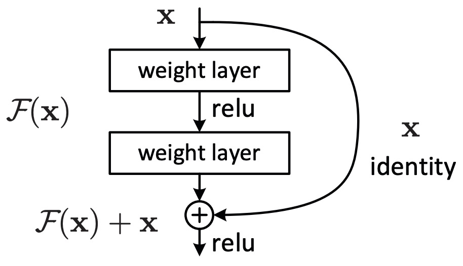
The following figure (source) shows the basic residual learning framework introduced in ResNet, where each block learns a residual function that is added to an identity shortcut rather than learning the complete transformation directly.
-
The identity shortcut ensures that the original representation always remains available. If the residual function learns zero, i.e., \(F(x)=0\), the block simply computes \(y=x\), recovering the identity mapping automatically.
-
This property explains why residual learning simplifies optimization. Instead of reconstructing representations from scratch, layers learn only the incremental corrections necessary to improve the current representation.
Anatomy of a residual block
-
A standard residual block consists of two parallel pathways:
-
The first is the identity shortcut \(x \rightarrow x\), which forwards the input unchanged.
-
The second is the residual branch \(x \rightarrow F(x)\), which performs one or more learnable transformations.
-
-
The outputs are combined through element-wise addition, \(y=x+F(x)\).
-
For convolutional ResNets:
\[F(x) = W_2 \sigma (W_1x)\]-
where:
- \(W_1\) and \(W_2\) denote convolutional layers.
- \(\sigma\) denotes a nonlinear activation such as ReLU.
-
-
In deeper bottleneck architectures,
\[F(x) = W_3 \sigma (W_2 \sigma (W_1x))\]-
using a sequence of:
- \(1 \times 1\) projection,
- \(3 \times 3\) convolution,
- \(1 \times 1\) expansion.
-
-
These bottleneck blocks significantly reduce computational cost while preserving representational capacity, allowing ResNet-50, ResNet-101, and ResNet-152 to scale efficiently.
Identity mapping
-
The defining feature of ResNet is the explicit identity shortcut.
-
Differentiating the residual block \(y=x+F(x)\), gives \(\frac{\partial y} {\partial x} = I+ \frac{\partial F} {\partial x}\).
-
Unlike ordinary feed-forward layers \(\frac{\partial y} {\partial x} = \frac{\partial F} {\partial x}\), the residual block always preserves the identity matrix.
-
Consequently:
-
Even when the learned transformation becomes small, i.e., \(\frac{\partial F} {\partial x} \approx 0\), gradients continue propagating through the identity pathway.
-
Identity Mappings in Deep Residual Networks by He et al. (2016) analyzed this property theoretically and experimentally, demonstrating that preserving an exact identity shortcut substantially improves optimization, especially for extremely deep networks.
Why residual learning works
- Residual learning provides several complementary benefits.
Easier optimization
-
Learning the residual \(F(x) = H(x)-x\) is frequently simpler than learning \(H(x)\) directly, particularly when the desired mapping is already close to the identity function.
-
Rather than reconstructing the entire representation, each layer modifies only those components requiring refinement.
Improved gradient propagation
-
Identity shortcuts introduce direct gradient pathways spanning many layers.
-
Rather than propagating exclusively through long chains of nonlinear transformations, gradients retain an unbroken identity route throughout the network.
Information preservation
-
Forward propagation also benefits.
-
Representations generated by earlier layers remain available to deeper layers regardless of how subsequent transformations behave.
-
This preservation reduces the likelihood that useful low-level information is permanently overwritten.
Implicit ensemble behavior
-
One influential interpretation views ResNet as an ensemble of relatively shallow computational paths.
-
Because gradients and information can traverse different combinations of residual blocks, the network effectively behaves like a collection of many shorter subnetworks rather than one extremely deep sequential chain.
-
Residual Networks Behave Like Ensembles of Relatively Shallow Networks by Veit et al. (2016) provided empirical evidence supporting this interpretation.
Projection shortcuts
-
The simple residual formulation assumes that the input and output possess identical dimensionality.
-
When channel counts differ, \(x \in \mathbb R^{d_1}, F(x) \in \mathbb R^{d_2}\), addition is no longer possible.
-
ResNet therefore introduces projection shortcuts, \(y = W_sx + F(x)\), where \(W_s\) is typically implemented as a \(1 \times 1\) convolution.
-
Projection shortcuts allow residual learning to accommodate changes in channel dimension or spatial resolution while preserving the shortcut pathway.
Residual learning versus Highway Networks
-
Residual Networks are closely related to Highway Networks, but differ in one important respect. Highway Networks compute \(y = (1-g) \odot x + g \odot F(x)\), where \(g\) is a learned gate. Instead, Residual Networks instead fix \(g=1\), yielding \(y=x+F(x)\).
-
Removing the gates substantially simplifies optimization while reducing computational overhead.
-
Empirically, this simpler formulation proved both easier to optimize and easier to scale.
Residual learning beyond convolutional networks
-
Although introduced for image recognition, residual learning rapidly became a universal architectural primitive.
-
Residual blocks now appear throughout modern machine learning:
-
CNNs employ additive residual blocks between convolutional stages.
-
Vision Transformers wrap both self-attention and feed-forward layers in residual pathways.
-
Large language models maintain persistent residual streams throughout every Transformer block.
-
Diffusion models employ residual blocks within U-Net backbones.
-
Graph neural networks increasingly rely on residual pathways to stabilize message passing across many graph layers.
-
-
The widespread adoption of residual learning illustrates that its success stems from general optimization principles rather than properties unique to computer vision.
Limitations of classical residual learning
-
Despite its remarkable success, the original ResNet formulation makes several assumptions that later work has begun to revisit.
-
Most importantly, every previous layer contributes equally through fixed identity addition.
-
For a deep residual network, \(h_l = h_1 + \sum_{i=1}^{l-1} f_i(h_i)\). Every layer therefore contributes with coefficient one, regardless of its relevance to the current computation. This uniform accumulation introduces several limitations. Earlier representations gradually become diluted as more residual updates accumulate. Different layer types cannot selectively emphasize different earlier representations. Residual topology remains fixed rather than learnable.
-
These observations motivated a new generation of residual architectures that reinterpret skip connections not merely as identity shortcuts but as adaptive mechanisms for information routing.
-
Hyper-Connections expand the residual stream into multiple interacting pathways, while Attention Residuals replace uniform accumulation with learned attention over preceding layer outputs. These developments retain the core insight introduced by ResNet, namely preserving stable information propagation, while substantially increasing the flexibility with which representations are routed across network depth.
Transition to dense connectivity
-
Residual Networks demonstrated that preserving identity pathways dramatically improves optimization. The next question naturally became whether representations should merely bypass intermediate layers or remain explicitly available to every subsequent layer.
-
This question motivated DenseNet, which replaced additive residual learning with dense concatenative connectivity. Rather than learning incremental corrections to a single residual stream, DenseNet allows every layer to directly access the complete set of feature maps produced by all preceding layers, emphasizing feature reuse rather than residual refinement. This alternative perspective further expanded the role of skip connections from optimization aids to mechanisms for preserving and exploiting intermediate representations throughout the network.
Skip Connections in the Transformer Architecture
-
Residual learning transformed the optimization of deep convolutional neural networks by introducing identity shortcuts that allowed information and gradients to propagate directly across depth. Although originally developed for computer vision, this architectural principle quickly proved to be much more general. When the Transformer architecture was introduced, residual connections became one of its fundamental building blocks, enabling stable optimization of increasingly deep sequence models. Today, every major large language model, including GPT, PaLM, Llama, Claude, Gemini, DeepSeek, Qwen, and Kimi, relies extensively on residual connections.
-
While the mathematical operation remains the same, residual connections play a substantially broader role in Transformer architectures than they do in ResNets. In convolutional networks, residual connections primarily stabilize optimization by allowing layers to learn residual corrections relative to their inputs. In Transformers, residual connections define a persistent computational substrate known as the residual stream, through which every component of the model communicates. Self-attention layers, feed-forward networks, mixture-of-experts modules, retrieval mechanisms, and other architectural components all read from this shared representation and write updates back into it. Consequently, the residual stream becomes the primary carrier of information throughout the network.
-
Understanding Transformer residual streams is essential for understanding modern LLMs. Recent architectures such as Hyper-Connections, Attention Residuals, and Manifold-Constrained Hyper-Connections all modify how information propagates through this residual stream rather than changing the attention mechanism itself. Before studying these newer architectures, it is therefore necessary to understand how residual connections are used within the Transformer.
Residual connections in the original Transformer
-
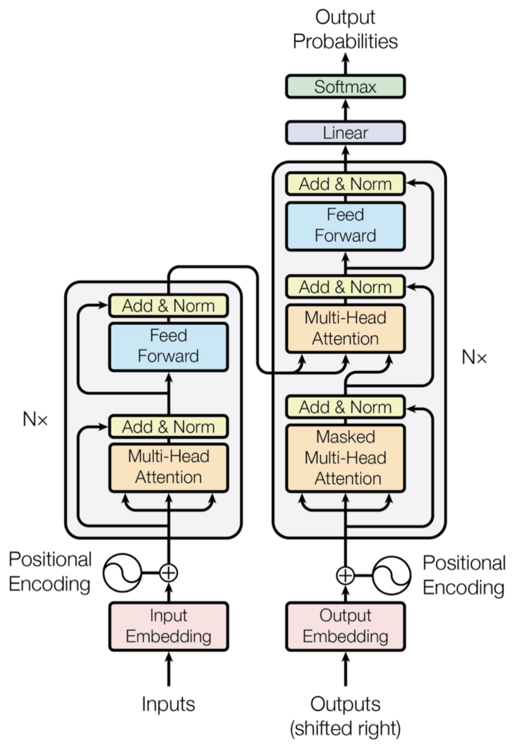
Attention Is All You Need by Vaswani et al. (2017) introduced the Transformer architecture, replacing recurrence with self-attention while retaining residual connections around every major sublayer. Each Transformer block consists of two principal components:
-
A multi-head self-attention layer that enables tokens to exchange information across the sequence. A position-wise feed-forward network (FFN) that independently transforms each token representation. Rather than replacing the current hidden representation, each component produces an incremental update that is added back to the residual stream.
-
The following figure (source) shows the original Transformer encoder and decoder architecture, illustrating residual connections surrounding both the multi-head attention and position-wise feed-forward sublayers.
-
For an input representation \(h_l\), the attention sublayer computes \(\tilde{h}_l = h_l + \text{Attention}(h_l)\), while the feed-forward network subsequently computes \(h_{l+1} = \tilde{h}_l + \text{FFN}(\tilde{h}_l)\).
-
Unlike ResNet, where a residual block typically contains several convolutional operations, Transformer architectures introduce a residual connection around every computational module. Consequently, each Transformer layer contributes multiple residual updates to the evolving hidden representation.
The residual stream
-
One of the most useful ways to interpret modern Transformers is to view them as operating on a persistent residual stream rather than as a sequence of independent hidden states.
-
Instead of each layer producing an entirely new representation, every module performs three conceptual operations:
-
Read the current residual stream.
-
Compute an incremental transformation.
-
Write the resulting update back into the residual stream.
-
-
Mathematically, the residual stream evolves as: \(h_{l+1} = h_l + \Delta_l\), where \(\Delta_l = f_l(h_l)\).
-
The key observation is that the hidden representation itself persists throughout the network. Individual layers modify this shared representation rather than replacing it entirely.
-
This interpretation has become increasingly important in mechanistic interpretability research. Rather than treating each Transformer layer as constructing an independent representation, researchers increasingly analyze how successive modules cooperate by reading from and writing to a common residual stream. Features introduced by early layers often remain accessible many layers later because they continue to exist within this accumulated representation.
Residual streams as persistent memory
-
The residual stream can be viewed as a form of distributed working memory that persists throughout the forward computation.
-
Attention layers primarily perform information routing across tokens, identifying which contextual information should influence each position.
-
Feed-forward networks primarily perform feature transformation, expanding and refining representations within each token independently.
-
Both modules communicate exclusively through the residual stream.
-
Consequently, the residual stream acts as the interface between all computations occurring within the model. Every architectural component contributes to a shared representation rather than maintaining isolated internal states.
-
This viewpoint explains why modern research increasingly focuses on the residual stream itself. If information becomes diluted, overwritten, or poorly routed within this shared representation, every downstream computation is affected.
Information accumulation across depth
-
Unlike ResNet, Transformer residual streams accumulate contributions from every preceding layer.
-
Expanding the recurrence yields: \(h_l = h_1 + \sum_{i=1}^{l-1} f_i(h_i)\).
-
Every attention layer and every feed-forward layer therefore contributes to a growing shared representation.
-
This additive accumulation has two important consequences:
-
First, useful information produced by early layers remains available throughout the network.
-
Second, later layers must operate on increasingly complex accumulated representations that contain contributions from every preceding computation.
-
-
This second property ultimately motivates architectures such as Attention Residuals. As depth increases, earlier representations become progressively diluted within the accumulated residual stream, making selective retrieval increasingly difficult.
Residual streams versus ResNet residuals
- Although both architectures employ additive identity mappings, their functional roles differ substantially.
| Property | ResNet | Transformer |
|---|---|---|
| Primary objective | Optimization | Optimization and persistent representation |
| Residual update | Convolutional block | Attention or FFN |
| Representation | Local feature maps | Shared hidden state |
| Communication | Between neighboring convolutional blocks | Between every computational module |
| Interpretation | Identity shortcut | Persistent residual stream |
-
In ResNet, the shortcut primarily exists to facilitate optimization.
-
In Transformers, the shortcut evolves into the central computational representation through which the entire model communicates.
-
This conceptual shift underlies many recent developments in Transformer architecture.
Limitations of residual accumulation
-
The original Transformer retains the same additive accumulation strategy introduced by ResNet.
-
Every layer contributes with coefficient one, \(h_l = h_1 + \sum_{i=1}^{l-1} f_i(h_i)\).
-
While remarkably successful, this formulation assumes that every previous layer should contribute equally to the current representation.
-
As model depth increases, two limitations emerge:
-
Hidden-state magnitudes tend to increase with depth, particularly in Pre-Norm Transformers.
-
Earlier representations become increasingly diluted within the accumulated residual stream.
-
-
Recent work such as Attention Residuals by Kimi Team et al. (2026) identifies these limitations as a consequence of fixed depth-wise aggregation and proposes replacing uniform residual accumulation with learned attention over previous layer outputs.
-
Before understanding these developments, however, we must first examine another major evolution of Transformer residual design: the transition from Post-Norm to Pre-Norm architectures, which fundamentally changed how normalization interacts with residual streams and laid the foundation for today’s frontier language models.
Pre-Norm and Post-Norm Skip Connections
-
The introduction of residual connections into the Transformer architecture solved many of the optimization challenges that had previously limited very deep neural networks. However, simply inserting residual pathways around attention and feed-forward layers was not sufficient to guarantee stable optimization at scale. A second design decision proved equally important: determining where normalization should be applied relative to the residual connection.
-
This seemingly minor architectural choice fundamentally changes how information propagates through the network. Early Transformer models normalized representations after each residual addition, a design now referred to as Post-Norm. While effective for relatively shallow architectures, Post-Norm becomes increasingly difficult to optimize as depth increases because gradients must traverse both the residual branch and the normalization layer. Subsequent work demonstrated that moving normalization before the residual computation dramatically improves optimization, giving rise to the Pre-Norm architecture used by nearly every modern large language model.
-
The transition from Post-Norm to Pre-Norm represents more than an implementation detail. It changes the dynamics of both forward information propagation and backward gradient flow, introduces new scaling behaviors in the residual stream, and ultimately motivates recent research on adaptive residual routing, including Attention Residuals. Understanding this evolution therefore provides the missing conceptual bridge between classical residual learning and the modern residual architectures discussed later in this primer.
The original Post-Norm Transformer
-
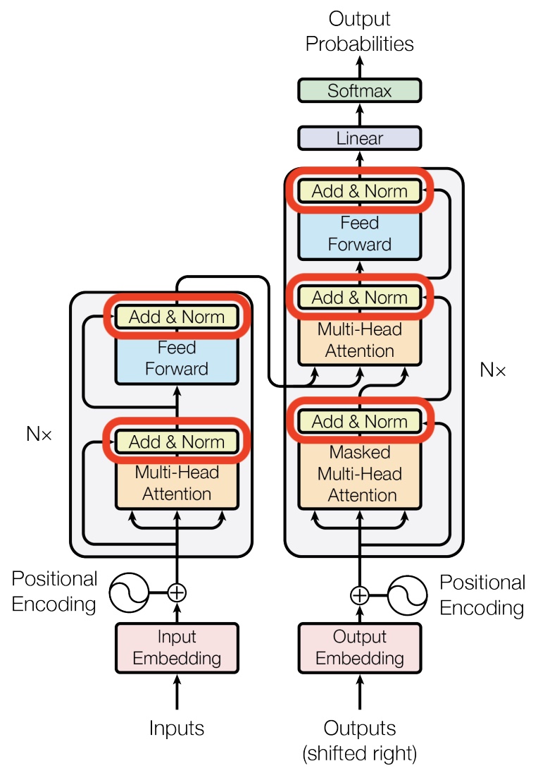
The Transformer introduced in Attention Is All You Need by Vaswani et al. (2017) applies Layer Normalization after each residual addition.
-
For an arbitrary sublayer, \(h_{l+1} = \mathrm{LayerNorm} \left(h_l + f_l(h_l) \right)\).
-
The following figure (source) shows the original Transformer architecture, where Layer Normalization is applied after each residual addition in both the encoder and decoder.
-
The computation proceeds in three stages:
-
The current residual stream is processed by a Transformer sublayer such as self-attention or a feed-forward network.
-
The resulting update is added to the residual stream.
-
Layer Normalization rescales the combined representation before it is passed to the next layer.
-
-
This formulation preserves the residual connection while maintaining normalized hidden-state statistics throughout the network.
-
Initially, Post-Norm proved sufficient because early Transformer models rarely exceeded a few dozen layers. However, as researchers attempted to train increasingly deeper models, optimization became progressively more unstable.
Layer Normalization
-
Normalization layers reduce sensitivity to activation scale by standardizing hidden representations before applying learnable affine transformations.
-
For an input vector \(x \in \mathbb{R}^{d}\), Layer Normalization computes:
\[\mathrm{LayerNorm}(x) = \gamma \frac{x-\mu} {\sqrt{\sigma^2+\epsilon}} + \beta\]- where \(\mu = \frac1d \sum_i x_i, \sigma^2 = \frac1d \sum_i (x_i-\mu)^2\).
-
Unlike Batch Normalization, Layer Normalization computes statistics independently for each token and therefore behaves consistently regardless of batch size or sequence length.
-
This property makes Layer Normalization particularly well suited for autoregressive language models.
Why Post-Norm becomes unstable
-
Although Post-Norm normalizes hidden states after every residual addition, it introduces an important drawback during backpropagation. Gradients must pass through \(\mathrm{LayerNorm}\) at every layer.
-
Consequently:
-
Unlike the residual shortcut introduced in ResNet, the identity pathway is no longer truly identity because every gradient must traverse the normalization operator.
-
As networks become deeper, this repeated normalization perturbs the clean gradient highway that originally motivated residual learning.
-
Empirically, researchers found that Post-Norm Transformers often require careful learning-rate warmup, extensive hyperparameter tuning, gradient clipping, conservative initialization, and to remain numerically stable during training.
-
These optimization challenges become increasingly severe beyond roughly several dozen Transformer layers.
The emergence of Pre-Norm
-
Subsequent work proposed moving normalization before each sublayer instead. The resulting architecture computes \(h_{l+1} = h_l + f_l (\mathrm{LayerNorm}(h_l))\).
-
Rather than normalizing the output of the residual addition, Pre-Norm normalizes only the input entering the nonlinear transformation. The residual shortcut itself remains untouched. Consequently:
-
The identity component now bypasses both the nonlinear transformation and the normalization layer. This restores the direct gradient pathway that made ResNet optimization remarkably effective.
-
Several influential language models, including GPT-2, GPT-3, PaLM, LLaMA, Claude, Gemini, Qwen, DeepSeek, and Kimi, all adopt Pre-Norm variants because of these optimization advantages.
Forward information propagation
-
Pre-Norm also changes how information accumulates throughout the network.
-
Because normalization is applied only to the residual branch, \(h_{l+1} = h_l + \Delta_l\), where \(\Delta_l = f_l (\mathrm{Norm}(h_l))\). Expanding the recurrence gives \(h_l = h_1 + \sum_{i=1}^{l-1} \Delta_i\). Unlike Post-Norm, the accumulated residual stream itself is never renormalized. Instead, every new update is added directly to the existing representation.
-
This property preserves information remarkably well but introduces a new phenomenon: the residual stream continually grows as additional updates accumulate.
Hidden-state growth
-
One consequence of Pre-Norm is that hidden-state magnitudes tend to increase with network depth. If each layer contributes approximately equal variance, \(\mathrm{Var}(h_l) \approx \sum_{i=1}^{l} \mathrm{Var}(\Delta_i)\), which grows approximately linearly with depth. The residual stream therefore becomes increasingly dominated by accumulated historical information.
-
Although this accumulation improves optimization, it also produces a subtle side effect. As the residual stream grows, earlier contributions become increasingly diluted, individual layer outputs contribute progressively smaller fractions of the overall representation, and distinguishing useful historical features becomes more difficult. This phenomenon is often referred to as Pre-Norm dilution.
-
Attention Residuals by Kimi Team et al. (2026) identifies this accumulation behavior as one of the principal limitations of fixed residual addition in modern LLMs. Rather than allowing every previous layer to contribute equally, Attention Residuals proposes learning adaptive depth-wise attention weights that selectively retrieve earlier representations.
RMSNorm
-
Many modern LLMs replace Layer Normalization with Root Mean Square Layer Normalization (RMSNorm).
-
RMSNorm: Root Mean Square Layer Normalization by Zhang and Sennrich (2019) observes that mean subtraction contributes relatively little to optimization stability. Instead, RMSNorm computes \(\mathrm{RMSNorm}(x) = \gamma \frac{x} {\sqrt{ \frac1d \sum_i x_i^2 + \epsilon}}\). Removing mean subtraction reduces computation while preserving nearly identical optimization behavior.
-
Today, RMSNorm is employed by most frontier LLMs, including LLaMA, DeepSeek, Qwen, Kimi, and many other decoder-only Transformer architectures.
Pre-Norm versus Post-Norm
- The practical differences between the two formulations can be summarized as follows.
| Property | Post-Norm | Pre-Norm |
|---|---|---|
| Normalization location | After residual addition | Before sublayer |
| Identity shortcut | Passes through normalization | True identity path |
| Gradient propagation | Harder at large depth | Stable across hundreds of layers |
| Hidden-state magnitude | Normalized after every layer | Accumulates across depth |
| Modern LLM usage | Rare | Nearly universal |
- The transition from Post-Norm to Pre-Norm illustrates a recurring theme in the evolution of residual architectures. Preserving a clean identity pathway substantially improves optimization, but doing so also changes how information accumulates throughout the network. The resulting residual stream becomes both more expressive and more challenging to manage.
Transition to adaptive residual routing
-
Pre-Norm solved one of the central optimization challenges facing deep Transformers by restoring an unimpeded identity path for gradient propagation. At the same time, its additive residual stream introduced a new limitation: every layer contributes uniformly to an ever-growing accumulated representation.
-
This observation raises a natural question. If attention mechanisms allow models to selectively retrieve information across sequence positions, why should residual connections continue to aggregate information across depth using fixed unit weights?
-
The remainder of this primer explores how recent architectures answer this question. Rather than treating residual addition as a fixed operation, they reinterpret the residual stream itself as an object that can be routed, weighted, constrained, and optimized. This evolution culminates in architectures such as Hyper-Connections, Attention Residuals, and Manifold-Constrained Hyper-Connections, which generalize the original ResNet identity shortcut into adaptive mechanisms for information routing across network depth.
Evolution of Skip Connections and Residual Connections
-
The development of skip connections over the past decade reflects a broader evolution in the role that connectivity plays within deep neural networks. Early skip connections were introduced primarily as optimization aids, allowing gradients to propagate more effectively through deep computational graphs. Over time, however, their role expanded considerably. Modern architectures increasingly treat skip connections as mechanisms for preserving representations, routing information, coordinating computation across layers, and improving systems efficiency. What began as a simple architectural shortcut has evolved into one of the central organizational principles of contemporary deep learning.
-
This evolution closely parallels the increasing scale of neural networks. Early convolutional models rarely exceeded a few dozen layers and primarily required stable optimization. Modern Transformer-based language models often contain hundreds of sequential layers, each operating on high-dimensional residual streams that accumulate information throughout the forward pass. As models became deeper, larger, and more computationally expensive, new challenges emerged that could no longer be addressed through fixed identity mappings alone. Recent research therefore seeks not to replace residual connections, but to generalize them into richer mechanisms for information routing across network depth.
-
This section traces that progression, showing how each generation of architectures builds upon the limitations of its predecessors.
From gated shortcuts to identity mappings
-
The earliest modern skip connections appeared in Highway Networks by Srivastava et al. (2015), which introduced learnable gates controlling how much information should bypass each layer. Inspired by gating mechanisms in recurrent neural networks, Highway Networks allowed representations to flow around nonlinear transformations when doing so improved optimization.
-
For an input representation \(x\), a Highway layer computes
\[y = T(x) \odot H(x) + (1-T(x)) \odot x\]-
where:
- \(H(x)\) is the transformed representation,
- \(T(x)\) is the learned transform gate,
- \(1-T(x)\) forms the carry gate.
-
-
The gates allow each layer to interpolate dynamically between preserving the input and applying a nonlinear transformation. Although effective, this flexibility comes at the cost of additional parameters and increased optimization complexity.
-
Residual Networks demonstrated that such gates were often unnecessary. Deep Residual Learning for Image Recognition by He et al. (2015) replaced learned interpolation with a fixed identity shortcut \(y=x+F(x)\), dramatically simplifying the architecture while achieving superior optimization and generalization. This observation established identity mappings as the dominant form of skip connection for deep neural networks.
From optimization to feature reuse
-
Residual learning emphasizes incremental refinement of a persistent representation. Shortly afterward, Densely Connected Convolutional Networks by Huang et al. (2017) proposed an alternative perspective in which every layer receives the complete set of feature maps produced by all preceding layers.
-
Instead of combining representations through addition,
\[h_l = [h_0,h_1,\ldots,h_{l-1}]\]- where \([\cdot]\) denotes concatenation.
-
This formulation encourages explicit feature reuse rather than residual refinement. Earlier representations remain directly accessible throughout the network, reducing redundant computation and improving parameter efficiency. DenseNet demonstrated that skip connections need not merely stabilize optimization; they can also improve representational efficiency by preserving intermediate features explicitly.
Long-range information preservation
-
The importance of skip connections became even more apparent in encoder-decoder architectures. Models such as U-Net: Convolutional Networks for Biomedical Image Segmentation by Ronneberger et al. (2015) introduced long-range skip connections linking encoder and decoder stages operating at matching spatial resolutions.
-
Unlike ResNet, whose shortcuts primarily improve optimization, U-Net skip connections preserve high-resolution spatial information that would otherwise be lost during repeated downsampling. These architectures demonstrated that skip connections can serve fundamentally different purposes depending on the computational task, ranging from optimization and feature reuse to information preservation and reconstruction.
Residual streams in Transformers
-
The introduction of the Transformer marked another important shift in the interpretation of skip connections. Rather than acting as isolated shortcuts around individual convolutional blocks, residual connections became the persistent computational substrate through which all modules communicate.
-
As discussed in the previous chapters, modern Transformer blocks repeatedly update a shared residual stream,
\[h_{l+1} = h_l + f_l(h_l)\]- where each self-attention layer and feed-forward network contributes an incremental update. The residual stream therefore becomes the model’s evolving representation rather than merely an optimization mechanism.
-
This reinterpretation greatly expands the significance of residual connections. Instead of preserving information across a small number of layers, they now coordinate computation across the entire network.
The limitations of fixed residual accumulation
-
Despite their remarkable success, classical residual connections retain one important assumption inherited from ResNet: every layer contributes equally to the evolving representation.
-
Expanding the recurrence gives
\[h_l = h_1 + \sum_{i=1}^{l-1} f_i(h_i)\] -
Each layer therefore contributes with an implicit coefficient of one. As Transformer depth increases, this fixed accumulation strategy introduces several limitations.
-
Earlier representations become progressively diluted within the accumulated residual stream. All previous layers contribute regardless of their relevance to the current computation.
-
Residual pathways remain fixed rather than adaptive. The residual stream grows continuously as additional updates are accumulated, particularly in Pre-Norm architectures.
-
These observations motivate a natural question: if attention mechanisms dynamically determine which tokens should communicate, should residual connections also determine dynamically which layers should contribute?
Toward adaptive residual routing
-
Recent research increasingly treats residual pathways as learnable communication structures rather than fixed architectural shortcuts. Several complementary directions have emerged.
-
Hyper-Connections generalize the single residual stream into multiple interacting streams connected through learned routing matrices, increasing the capacity of the residual topology itself (Hyper-Connections by Zhu et al. (2024)).
-
Attention Residuals reinterpret residual accumulation as an attention mechanism over depth, allowing each layer to retrieve earlier representations selectively instead of relying on uniform addition (Attention Residuals by Kimi Team et al. (2026)).
-
Manifold-Constrained Hyper-Connections constrain learned residual routing to the manifold of doubly stochastic matrices, preserving the stability properties that originally made identity mappings successful while retaining the expressive capacity of multi-stream routing (mHC: Manifold-Constrained Hyper-Connections by Xie et al. (2025)).
-
Collectively, these architectures represent a fundamental shift in the design philosophy of residual networks. Instead of asking how information can bypass intermediate layers, they ask how information should be routed, weighted, preserved, and combined throughout increasingly deep networks.
A unifying perspective
-
Viewed historically, the evolution of skip connections reflects a gradual expansion of their role within neural architectures:
-
Highway Networks introduced learnable shortcuts to improve optimization.
-
ResNet simplified these shortcuts into fixed identity mappings that enabled extremely deep networks.
-
DenseNet emphasized explicit feature reuse through dense concatenation.
-
U-Net demonstrated the importance of long-range information preservation.
-
Transformers elevated residual pathways into persistent computational streams shared by every module.
-
-
Hyper-Connections, Attention Residuals, and Manifold-Constrained Hyper-Connections reinterpret residual pathways themselves as adaptive routing mechanisms.
-
This progression illustrates that skip connections are no longer merely shortcuts around computation. They have become the primary mechanism through which modern neural networks organize, preserve, and communicate information across depth.
-
The following sections examine these recent developments in detail, beginning with DenseNet and U-Net before exploring how contemporary architectures generalize residual learning beyond fixed identity mappings toward adaptive, learnable residual routing.
DenseNet
-
Residual Networks demonstrated that identity mappings dramatically improve the optimization of deep neural networks by allowing each layer to learn an incremental correction to its input. However, residual learning preserves only the current hidden representation. Once a layer has transformed its input, earlier intermediate feature maps are no longer directly accessible unless they are implicitly preserved within the residual stream. This raises an important question: if intermediate representations remain useful throughout the network, why not expose them explicitly to every subsequent layer rather than repeatedly compressing them into a single residual state?
-
Densely Connected Convolutional Networks by Huang et al. (2017) answers this question by replacing additive residual learning with dense feature reuse. Instead of forwarding only the output of the previous layer, every layer receives the feature maps produced by every preceding layer through concatenative skip connections. This dense connectivity fundamentally changes the role of skip connections. Rather than serving primarily as optimization shortcuts, they become a mechanism for preserving and reusing learned representations throughout the network.
-
DenseNet demonstrates that skip connections need not always merge information through addition. By explicitly retaining intermediate representations, dense connectivity encourages feature reuse, reduces redundant computation, and improves parameter efficiency. Although DenseNet was originally proposed for convolutional image recognition, its underlying philosophy, namely that useful intermediate representations should remain accessible rather than repeatedly reconstructed, continues to influence modern neural architectures.
Motivation
- Residual learning assumes that each layer should refine a shared representation by learning an additive correction:
-
While this formulation greatly improves optimization, it still compresses all previously learned information into a single hidden representation. Every subsequent layer therefore operates on the current residual state rather than the complete collection of previously computed features.
-
As network depth increases, this repeated compression may cause useful representations learned early in the network to become increasingly difficult to recover. Even though residual connections preserve an identity pathway, individual feature maps are continually merged into the evolving hidden state.
-
DenseNet takes a different perspective. Rather than repeatedly transforming a single representation, every newly computed feature map becomes part of a growing collection that remains directly accessible throughout the remainder of the network. Later layers therefore reuse previously computed features instead of reconstructing them.
Dense connectivity
-
Unlike ResNet, where each layer receives only the immediately preceding representation, DenseNet connects every layer to every subsequent layer.
-
For the \(l^{th}\) layer,
\[h_l = F_l \left( [h_0,h_1,\ldots,h_{l-1}] \right)\]- where \([\cdot]\) denotes concatenation along the channel dimension.
-
The following figure (source) shows the connectivity pattern of DenseNet, illustrating how each layer receives the concatenated feature maps produced by every preceding layer rather than only the previous layer.
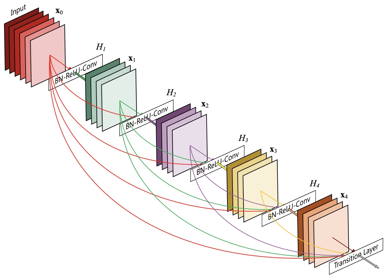
- Unlike residual learning, where earlier information is merged through addition \(h_l = h_{l-1} + F_{l-1}\), dense connectivity preserves every feature map explicitly. Consequently, the input dimensionality of each layer grows throughout the network.
Feature reuse
-
The defining principle behind DenseNet is explicit feature reuse.
-
Each convolutional layer receives access to low-level edge detectors, intermediate texture representations, higher-level semantic features, and all previously computed feature maps.
-
Rather than relearning similar representations repeatedly, layers selectively build upon existing features. This produces several advantages:
-
Low-level features remain available throughout the network.
-
Intermediate representations are preserved without approximation.
-
Later layers can specialize instead of reconstructing earlier computations.
-
Redundant feature extraction is substantially reduced.
-
-
The authors demonstrate that many learned feature maps continue to be reused dozens of layers after they are first computed, suggesting that earlier representations retain long-term value throughout the network.
Growth rate
-
Since every layer contributes additional feature maps, the number of channels increases monotonically with depth.
-
Suppose each layer contributes \(k\) new feature maps. Then after \(L\) layers, \(C_L = C_0 + kL\), where \(C_0\) is the number of input channels. The parameter \(k\) is known as the growth rate.
-
Unlike conventional CNNs, whose width often doubles between stages, DenseNet allows representational capacity to increase gradually by introducing only a small number of new feature maps per layer. Typical values include: \(k=12,\;24,\;32\).
-
A relatively small growth rate is sufficient because every layer has access to all previously computed features.
Dense blocks
-
Dense connectivity is implemented within structures known as dense blocks. Inside each block, every layer receives all preceding feature maps, every layer contributes new feature maps, and feature dimensionality grows linearly. The output of a dense block therefore contains \(C_0 + kL\) channels.
-
The following figure (source) shows a deep DenseNet with three dense blocks. The layers between two adjacent blocks are referred to as transition layers and change feature-map sizes via convolution and pooling.

- Between dense blocks, DenseNet inserts transition layers consisting of Batch Normalization, \(1 \times 1\) convolution, and 2×2 average pooling. These transition layers reduce feature dimensionality and spatial resolution, preventing channel growth from becoming prohibitively expensive.
Bottleneck layers and compression
-
Although dense connectivity improves feature reuse, naïvely concatenating feature maps would eventually become computationally expensive.
-
To mitigate this growth, DenseNet introduces bottleneck layers. Each dense layer computes \(1\times1 \rightarrow 3\times3\) convolutions. The \(1 \times 1\) projection first reduces channel dimensionality, after which the computationally expensive \(3 \times 3\) convolution operates on the compressed representation.
-
Additionally, transition layers apply a compression factor \(\theta \in (0,1]\), producing \(C_{\mathrm{out}} = \theta C_{\mathrm{in}}\).
-
Typical implementations employ \(\theta=0.5\), approximately halving the number of channels between dense blocks.
-
These design choices make DenseNet computationally practical despite its extensive connectivity.
Comparison with residual learning
- Although DenseNet and ResNet both employ skip connections, they solve different problems.
| Property | ResNet | DenseNet |
|---|---|---|
| Skip operation | Addition | Concatenation |
| Hidden dimension | Constant | Grows with depth |
| Primary objective | Residual refinement | Feature reuse |
| Information preservation | Implicit through residual stream | Explicit through concatenation |
| Parameter efficiency | Good | Excellent |
-
Residual Networks preserve optimization by maintaining a persistent hidden representation that is gradually refined.
-
DenseNet instead preserves every intermediate representation explicitly, allowing later layers to determine which features remain useful.
-
One architecture emphasizes iterative refinement, while the other emphasizes feature accumulation.
Strengths and limitations
-
Dense connectivity offers several notable advantages:
-
Excellent gradient propagation due to short paths between all pairs of layers.
-
Extensive feature reuse throughout the network.
-
Improved parameter efficiency compared to similarly accurate ResNets.
-
Strong performance on relatively small datasets where feature reuse is particularly valuable.
-
-
However, dense connectivity also introduces important tradeoffs:
-
Feature dimensionality increases throughout each dense block.
-
Memory consumption grows because all intermediate feature maps must remain available.
-
Concatenation increases communication overhead during distributed training.
-
Computational efficiency decreases for extremely deep networks because channel growth eventually dominates.
-
-
These limitations have largely prevented DenseNet-style connectivity from being adopted in modern large language models, where hidden dimensionality and activation memory already constitute major bottlenecks.
Influence on later architectures
-
Although DenseNet itself is less common in today’s frontier foundation models, its underlying principle of preserving intermediate representations has had lasting influence.
-
Encoder-decoder architectures such as U-Net employ concatenative skip connections to recover fine-grained spatial information during decoding.
-
Feature pyramid networks aggregate multi-scale representations using similar ideas.
-
Recent Transformer research increasingly revisits explicit feature preservation, although typically through adaptive routing mechanisms rather than literal concatenation.
-
In this sense, DenseNet represents an important alternative branch in the evolution of skip connections. Whereas ResNet showed that optimization improves when layers learn residual corrections, DenseNet demonstrated that representation learning improves when useful features remain directly accessible throughout the network.
-
The next section explores another influential use of skip connections in encoder-decoder architectures. Unlike DenseNet, which emphasizes feature reuse across depth, U-Net employs long-range skip connections to preserve spatial detail across changes in resolution, illustrating yet another role that skip connections can play in modern neural network design.
U-Net and Long Skip Connections
-
Residual Networks and DenseNet demonstrated that skip connections substantially improve optimization and feature reuse within feed-forward architectures. Both models, however, operate primarily on networks that preserve a single forward computational direction. Encoder-decoder architectures introduce a different challenge. Rather than maintaining a constant feature resolution throughout the network, they repeatedly compress the input into increasingly abstract representations before reconstructing a high-resolution output. While this hierarchical encoding enables large receptive fields and rich semantic understanding, it also progressively discards fine-grained spatial information that is often essential for dense prediction tasks such as semantic segmentation, medical image analysis, depth estimation, and image restoration.
-
This observation motivated a new class of skip connections designed not to improve optimization alone, but to preserve information lost during changes in spatial resolution. U-Net: Convolutional Networks for Biomedical Image Segmentation by Ronneberger et al. (2015) introduced long-range encoder-decoder skip connections that directly transfer high-resolution feature maps from the encoder to corresponding decoder stages. These connections allow the decoder to combine coarse semantic information with fine spatial detail, enabling accurate localization without sacrificing contextual understanding.
-
Unlike the local residual shortcuts introduced in ResNet or the dense feature reuse of DenseNet, U-Net demonstrates that skip connections can bridge entirely different stages of a network. This expanded view significantly broadened the role of skip connections, showing that they can preserve information not only across depth but also across changes in representation scale.
Motivation
-
Many vision problems require predictions at the same spatial resolution as the input image.
-
Examples include semantic segmentation, instance segmentation, medical image segmentation, image matting, optical flow, monocular depth estimation, image restoration, etc.
-
These tasks require two complementary forms of information:
-
Global semantic understanding, which identifies the objects or regions present in the image.
-
Fine spatial detail, which precisely delineates boundaries and small structures.
-
-
Encoder-decoder architectures naturally capture semantic information through repeated downsampling, increasing the receptive field and allowing each neuron to integrate information from larger image regions. However, each downsampling operation inevitably reduces spatial resolution.
-
Consequently, the decoder receives highly abstract representations that often lack the precise localization required for pixel-level prediction.
-
Long skip connections address this problem by directly forwarding high-resolution encoder features to matching decoder stages.
Encoder-decoder architecture
-
A typical encoder-decoder network consists of two complementary pathways.
-
The encoder progressively reduces spatial resolution while increasing semantic abstraction:
-
The decoder performs the reverse process,
\[\frac{H}{2^L} \times \frac{W}{2^L} \rightarrow \cdots \rightarrow H \times W\]- gradually reconstructing the original image resolution.
-
Although the decoder recovers spatial dimensions through upsampling, information discarded during pooling or strided convolutions cannot be recovered perfectly.
-
The following figure (source) shows the U-Net architecture, illustrating the symmetric encoder-decoder structure connected by long-range skip connections between corresponding resolution levels.
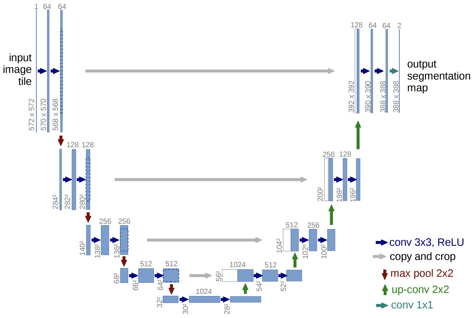
Long skip connections
-
U-Net solves this information loss by introducing skip connections between encoder and decoder stages operating at identical spatial resolutions.
-
Suppose \(e_i\) denotes the encoder feature map at level \(i\), and \(d_i\) denotes the corresponding decoder representation. The decoder computes \(d_i=F_i([d_i; e_i])\), where \([\cdot]\) denotes channel-wise concatenation.
-
Unlike residual learning \(x+F(x)\), U-Net preserves encoder features explicitly through concatenation. Consequently, high-resolution edge information, boundary localization, texture, fine spatial structure, and remain directly available during reconstruction.
-
The decoder therefore refines semantic representations rather than attempting to reconstruct lost spatial detail from scratch.
Why concatenation instead of addition?
-
An important design choice in U-Net is the use of concatenation rather than residual addition. Suppose \(e_i, d_i \in \mathbb{R}^{C\times H\times W}\). Residual addition would compute \(d_i+e_i\), forcing both representations to merge immediately. Instead, concatenation produces \([e_i;d_i] \in \mathbb{R}^{2C\times H\times W}\), preserving both representations independently.
-
Subsequent convolutions determine how these complementary features should be integrated. This design provides considerably greater flexibility because semantic decoder features and high-resolution encoder features often encode fundamentally different information.
Information preservation across scale
-
Unlike ResNet and DenseNet, whose skip connections primarily preserve information across depth, U-Net preserves information across changes in spatial resolution.
-
Repeated pooling discards precise object boundaries, thin structures, small anatomical details, local texture, and pixel-level alignment.
-
Long skip connections bypass these irreversible operations entirely. Consequently, information that would otherwise be destroyed remains available throughout decoding. This distinction illustrates an important general principle. Skip connections preserve whatever information would otherwise be difficult to reconstruct.
-
Depending on the architecture, this may include: gradients, feature maps, hidden representations, spatial detail, residual streams, or learned routing information.
Multi-scale feature fusion
-
One interpretation of U-Net is that it performs multi-scale feature fusion.
-
Each decoder stage combines coarse semantic representations from deeper layers, and increasingly fine spatial representations from shallower encoder stages. This allows predictions to incorporate both global context and local precision simultaneously.
-
Many subsequent architectures extend this idea. Examples include Feature Pyramid Networks (FPN), PANet, HRNet, DeepLab variants, Mask R-CNN, etc.
-
Although these models differ architecturally, they all exploit long skip connections to combine information across multiple spatial scales.
Comparison with other skip connections
- The three major skip-connection paradigms introduced so far emphasize different objectives.
| Architecture | Skip operation | Primary purpose |
|---|---|---|
| ResNet | Addition | Stable optimization through residual learning |
| DenseNet | Concatenation across depth | Explicit feature reuse |
| U-Net | Concatenation across encoder-decoder stages | Preservation of spatial information |
-
This comparison highlights that skip connections should not be viewed as a single architectural mechanism.
-
Instead, they represent a family of information-preserving connectivity patterns tailored to different computational objectives.
Strengths and limitations
-
Long skip connections offer several advantages:
-
Preserve fine spatial detail throughout decoding.
-
Improve localization accuracy for dense prediction.
-
Enable efficient integration of global context and local structure.
-
Reduce the burden on decoder layers by avoiding repeated reconstruction of lost features.
-
-
However, they also introduce several tradeoffs:
-
High-resolution feature maps must be retained until decoding, increasing activation memory.
-
Concatenation increases channel dimensionality, requiring additional computation.
-
Skip connections assume a correspondence between encoder and decoder resolutions, limiting architectural flexibility.
-
Communication overhead increases in distributed implementations because large feature maps must remain available.
-
-
Despite these costs, long skip connections remain the dominant architectural choice for segmentation, image restoration, and many dense prediction problems.
Influence on modern architectures
-
Although U-Net was developed for biomedical image segmentation, its central insight extends well beyond medical imaging.
-
Modern diffusion models, including Stable Diffusion and many latent diffusion architectures, employ U-Net backbones whose long skip connections preserve high-resolution image information throughout the denoising process.
-
Vision Transformers increasingly incorporate multi-scale skip pathways inspired by encoder-decoder architectures.
-
Even recent large multimodal models employ hierarchical feature fusion strategies that resemble long skip connections, allowing visual representations computed at different resolutions to interact during decoding.
-
These developments reinforce a broader lesson emerging throughout this primer: skip connections are not merely optimization shortcuts. They are mechanisms for preserving information that would otherwise become inaccessible during computation.
Transition to modern residual architectures
-
By this point in the evolution of skip connections, three complementary design philosophies had emerged:
-
ResNet demonstrated that additive identity mappings dramatically improve optimization.
-
DenseNet showed that preserving intermediate feature maps explicitly encourages feature reuse and parameter efficiency.
-
U-Net illustrated that long-range skip connections preserve spatial information across changes in representation scale.
-
-
Together, these architectures established skip connections as a fundamental mechanism for preserving information throughout deep neural networks. However, they also shared one important characteristic: the connectivity pattern itself remained fixed.
-
Recent Transformer architectures revisit this assumption. Rather than treating skip connections as static pathways, they learn how information should be routed across depth. The next chapters examine this evolution, beginning with Attention Residuals, which reinterpret residual accumulation itself as an attention mechanism operating over previous layers, and continuing with Hyper-Connections and Manifold-Constrained Hyper-Connections, which generalize the residual stream into learnable multi-stream routing architectures.
Attention Residuals
-
The success of residual learning transformed deep neural network optimization by establishing identity mappings as the primary mechanism for propagating information across depth. Transformer architectures inherited this principle almost unchanged, replacing convolutional residual blocks with residual streams surrounding self-attention and feed-forward layers. Combined with the transition from Post-Norm to Pre-Norm Transformers, this formulation enabled the stable training of models containing hundreds of layers and hundreds of billions of parameters.
-
Despite this remarkable success, the residual stream retained a fundamental assumption inherited directly from ResNet: every preceding layer contributes equally to the hidden representation through fixed additive accumulation. While this assumption was well suited to relatively shallow convolutional networks, it becomes increasingly restrictive as Transformer depth grows. Modern large language models continuously accumulate representations from attention layers, feed-forward networks, mixture-of-experts blocks, retrieval modules, and other computational components into a single residual stream. Consequently, later layers must operate on hidden representations containing the cumulative contributions of every previous layer, regardless of whether those earlier representations remain relevant to the current computation.
-
This observation motivated a new interpretation of residual connections. Rather than viewing the residual stream as a passive accumulation of intermediate representations, recent work asks whether it should instead behave like an adaptive memory system. Just as self-attention enables tokens to retrieve the most relevant information across sequence positions, residual connections might similarly retrieve the most useful representations across network depth.
-
Attention Residuals by Kimi Team et al. (2026) develops this idea by replacing fixed residual addition with attention over previous layer outputs. Instead of uniformly accumulating every residual update with coefficient one, each layer learns to retrieve earlier representations selectively according to the current computational context. This reinterpretation transforms residual learning from static information accumulation into adaptive depth-wise information routing while preserving the optimization advantages that originally motivated residual connections.
Motivation
-
The Pre-Norm Transformer maintains a residual stream whose hidden representation evolves according to \(h_{l+1} = h_l + f_l(h_l)\).
-
Expanding this recurrence yields: \(h_l = h_1 + \sum_{i=1}^{l-1} f_i(h_i)\).
-
Every layer therefore contributes equally to the accumulated representation.
-
This formulation possesses several desirable properties:
-
Information produced by early layers remains available throughout the network.
-
Identity mappings continue to facilitate stable gradient propagation.
-
Every layer performs only an incremental refinement of the existing representation.
-
-
However, as Transformer depth increases, uniform accumulation also introduces several limitations.
Uniform accumulation treats every layer equally
-
The additive residual stream assigns identical weight to every previous layer regardless of its relevance.
-
Consequently, shallow syntactic representations, intermediate semantic abstractions, high-level reasoning features, and all contribute equally to the hidden state.
-
Unlike sequence attention, which dynamically determines which tokens should communicate, residual accumulation cannot distinguish between useful and irrelevant intermediate representations.
Earlier representations become progressively diluted
-
As the residual stream grows, \(h_l = h_1 + \sum_{i=1}^{l-1} f_i(h_i)\), the relative contribution of any single layer decreases approximately as \(\frac{1}{l}\).
-
Although earlier representations remain mathematically present, they become increasingly difficult to isolate because they are embedded within an ever-growing accumulated state.
-
This phenomenon is particularly pronounced in Pre-Norm Transformers, where the residual stream itself is never renormalized.
Fixed accumulation cannot adapt to different computations
-
Different Transformer layers often perform qualitatively different computations:
-
Early layers typically encode lexical and syntactic information.
-
Intermediate layers construct semantic representations.
-
Later layers increasingly perform reasoning, planning, and task-specific computation.
-
-
A fixed additive residual stream assumes that every stage should receive identical contributions from all preceding layers.
-
Intuitively, however, reasoning layers might benefit more from intermediate semantic representations than from very early lexical features, while syntactic refinement may primarily depend upon nearby layers.
-
Uniform accumulation cannot express these preferences.
From residual addition to depth-wise attention
-
The central insight of Attention Residuals is that residual accumulation can be interpreted as a special case of attention operating over network depth.
-
Instead of accumulating \(h_l = h_1 + \sum_{i=1}^{l-1} f_i(h_i)\), each layer retrieves a weighted combination of previous representations, as follows:
\[h_l = \sum_{i=0}^{l-1} \alpha_{i\rightarrow l} v_i\]-
where:
\[\sum_i \alpha_{i\rightarrow l} = 1\]- where, \(v_0=h_1\), while \(v_i=f_i(h_i), i \ge 1\).
-
-
The coefficients \(\alpha_{i\rightarrow l}\) are learned attention weights rather than fixed constants. This simple modification fundamentally changes the role of residual connections.
-
Instead of functioning as a passive accumulation mechanism, the residual stream becomes an adaptive retrieval system capable of selecting information generated at different depths.
-
The following figure (source) shows an overview of Attention Residuals, comparing standard residual accumulation with Full Attention Residuals and Block Attention Residuals, illustrating how residual connections are generalized into learned attention over previous layer outputs.
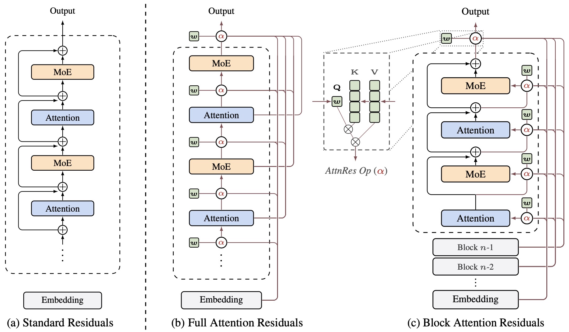
Residual connections as linear attention
-
An important conceptual contribution of the paper is the observation that classical residual connections already resemble a degenerate form of attention.
-
Standard residual accumulation can be rewritten as: \(h_l=\sum_{i=0}^{l-1}\frac{1}{l} v_i\). This corresponds to attention with uniform weights, \(\alpha_{i\rightarrow l}=\frac{1}{l}\). In other words, every previous layer is attended equally, attention scores are independent of the current computation, and routing decisions never change across inputs.
-
Attention Residuals therefore do not replace residual learning. Instead, they generalize it.
-
Standard residual addition becomes one particular operating point within a much larger family of depth-wise attention mechanisms.
-
This perspective closely parallels the historical transition from recurrent neural networks to self-attention. Just as self-attention generalized fixed sequential recurrence into adaptive communication across sequence positions, Attention Residuals generalize fixed residual accumulation into adaptive communication across network depth.
Depth-wise attention formulation
-
Attention Residuals employ the familiar query-key-value formulation used throughout Transformer architectures, but apply it across layers instead of sequence positions.
-
For each layer \(q_l = w_l\), where \(w_l \in \mathbb{R}^d\) is a learned pseudo-query associated with layer \(l\).
-
Keys correspond to normalized previous layer outputs \(k_i = \mathrm{RMSNorm}(v_i)\), while values are simply \(v_i\).
-
Attention weights are computed as:
- The residual stream is then formed as:
-
Unlike conventional self-attention, queries depend only on layer identity, keys and values depend on previous layer outputs, attention operates across depth rather than tokens.
-
This design preserves parallel computation while enabling adaptive routing across the network.
Why pseudo-queries?
-
One of the most distinctive implementation choices is the use of learned pseudo-query vectors rather than computing queries from hidden representations.
-
This design offers several practical advantages:
-
Query computation is independent of the current forward activations.
-
All depth-attention weights can therefore be computed simultaneously.
-
Pipeline parallelism remains efficient because query vectors need not be communicated between devices.
-
Additional computational overhead is minimal, requiring only one learnable vector per layer.
-
Although simple, this design significantly improves scalability compared to fully activation-dependent depth attention.
-
Interpretation
-
Attention Residuals fundamentally change how residual streams should be understood.
-
Rather than viewing the hidden state as an accumulated sum of previous updates, \(h_l = h_1 + \sum_i f_i(h_i)\), the residual stream becomes a learned memory over network depth.
-
Each layer effectively asks:
Which previous representations are most useful for the computation I am about to perform?
-
This interpretation elevates residual connections from optimization mechanisms to adaptive retrieval systems.
-
In this sense, Attention Residuals play a role analogous to self-attention. Self-attention retrieves information across sequence positions. Attention Residuals retrieve information across network depth. Both replace fixed communication patterns with learned routing policies.
Advantages over classical residual connections
-
Replacing fixed accumulation with learned depth-wise attention provides several important benefits:
-
Earlier representations remain directly retrievable rather than becoming diluted within an accumulated residual stream.
-
Different layers can retrieve different combinations of previous computations depending on their functional role.
-
Hidden-state magnitudes remain more balanced across depth because representations are normalized before attention.
-
Information routing becomes adaptive without sacrificing the optimization advantages of residual learning.
-
-
Empirical results presented in the paper demonstrate improvements across multiple model scales while maintaining stable optimization, suggesting that adaptive depth-wise routing offers a promising generalization of classical residual learning.
Transition to scalable implementations
-
While Full Attention Residuals provide the most expressive formulation, they require every layer to attend over every previous layer. As model depth increases into the hundreds of layers typical of modern frontier language models, this quadratic dependence introduces additional computation, memory, and communication costs.
-
The next section addresses this challenge by introducing Block Attention Residuals, which approximate full depth-wise attention using hierarchical block-level summaries. This formulation preserves most of the representational benefits of adaptive residual routing while making the approach practical for large-scale distributed training.
Block Attention Residuals
-
The formulation introduced in the previous section provides a conceptually elegant generalization of residual learning by allowing each layer to attend over all previous layer outputs. However, this expressivity comes at a computational cost. Unlike standard residual connections, whose computational complexity grows linearly with network depth, Full Attention Residuals require every layer to compare itself against every preceding layer. Although Transformer depth is considerably smaller than sequence length, frontier language models commonly contain one hundred or more layers, making naïve depth-wise attention increasingly expensive during both training and distributed inference.
-
The primary challenge is therefore not whether adaptive residual routing improves representation learning, but whether it can be implemented efficiently at modern model scales. Large language model training is often limited not by floating-point computation but by memory bandwidth and inter-device communication. Consequently, any new architectural component must be designed with systems considerations in mind.
-
To address this challenge, Attention Residuals by Kimi Team et al. (2026) introduces Block Attention Residuals (Block AttnRes), a hierarchical approximation that dramatically reduces communication and memory overhead while preserving nearly the same expressive power as Full Attention Residuals. Rather than attending over every previous layer individually, Block AttnRes organizes layers into blocks and performs attention over block summaries, followed by lightweight refinement within each block. This hierarchical organization transforms depth-wise attention into a scalable operation suitable for distributed training of frontier-scale language models.
Motivation
-
Suppose a Transformer contains \(L\) layers. Full Attention Residuals compute:
\[h_l = \sum_{i=0}^{l-1} \alpha_{i\rightarrow l} v_i\]- requiring every layer to maintain access to all previous representations.
-
This introduces several practical challenges:
-
Every intermediate layer output must remain available throughout the forward pass.
-
Pipeline-parallel training requires transmitting all previous layer outputs across pipeline stages.
-
Memory access becomes increasingly expensive as the number of stored representations grows.
-
Communication overhead begins to dominate computation on modern accelerator clusters.
-
-
These limitations are particularly important because contemporary LLM training is frequently constrained by memory bandwidth rather than arithmetic throughput.
-
The paper therefore asks whether every previous layer truly needs to participate independently in the attention computation.
Hierarchical residual aggregation
-
Block Attention Residuals address this problem by partitioning the network into \(N\) blocks, each containing \(S=\frac{L}{N}\) layers.
-
Instead of attending over individual layer outputs, the model first summarizes the completed layers within each block.
-
For block \(B_n\), the block representation is:
-
These block summaries become the units over which inter-block attention operates.
-
The following figure (source) shows the PyTorch-style implementation of Block Attention Residuals, illustrating how completed block summaries are combined with partial within-block residual states during the forward computation.
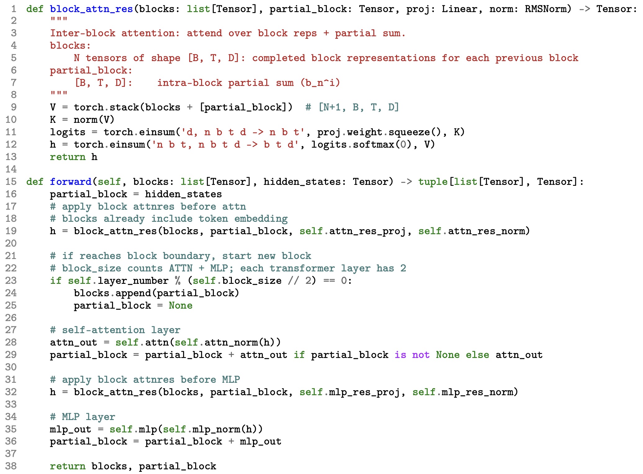
- Rather than retrieving hundreds of individual layer outputs, each layer retrieves only a relatively small number of block summaries together with the partial computations from its current block.
Two-level attention
- Block Attention Residuals divide computation into two complementary stages.
Inter-block attention
- Completed blocks are treated as high-level memory units. Attention is computed over \(N\) block summaries:
-
Since \(N \ll L\), this dramatically reduces the size of the attention problem.
-
Each completed block summarizes the information produced by many preceding layers while remaining inexpensive to store and communicate.
Intra-block refinement
-
Within the current block, individual layer outputs remain available explicitly.
-
The current layer therefore also attends to the partially accumulated representations inside its own block, producing \(h_l^{(\mathrm{intra})}\).
-
The final residual representation combines both sources of information,
-
Intuitively, completed blocks provide long-range historical context and current-block representations preserve fine-grained local information.
-
This hierarchy closely resembles multi-scale feature aggregation used elsewhere in deep learning.
Online softmax merging
-
Simply concatenating inter-block and intra-block attention outputs would produce incorrect normalization because each attention computation is normalized independently.
-
Instead, Block Attention Residuals employ an online softmax formulation that exactly reconstructs the result obtained by performing attention jointly over all representations.
-
Suppose \((o^{(1)},\ell^{(1)})\) represent the output and normalization term produced by inter-block attention, while \((o^{(2)},\ell^{(2)})\) represent the corresponding quantities for intra-block attention.
-
The merged output becomes:
\[h_l = \frac{ e^{m_1-m} o^{(1)} + e^{m_2-m} o^{(2)} } { e^{m_1-m} \ell^{(1)} + e^{m_2-m} \ell^{(2)} },\]- where \(m = \max(m_1,m_2)\) improves numerical stability.
-
This formulation produces the same result as full attention while avoiding the need to materialize every previous layer simultaneously.
Computational complexity
-
The principal advantage of Block Attention Residuals is improved scalability.
-
Suppose
- \(L\) denotes the number of layers,
- \(N\) denotes the number of blocks,
- \(d\) denotes the hidden dimension.
-
Full Attention Residuals:
- Computation:
- Memory:
-
Block Attention Residuals:
- Computation:
- Memory:
-
Since \(N \ll L\), both memory consumption and communication decrease substantially.
-
Importantly, this reduction comes with only a modest approximation because completed blocks capture most of the information contained in earlier layers.
Systems-aware implementation
-
One of the most distinctive aspects of the paper is its emphasis on systems optimization.
-
Unlike many architectural proposals that focus primarily on modeling improvements, Attention Residuals explicitly consider the practical constraints of distributed LLM training.
Batched inter-block attention
- All layers within a block share the same set of completed block summaries. Consequently, attention for every layer inside a block can be computed simultaneously, forming matrices:
- Batching these operations amortizes memory access across multiple layers, improving accelerator utilization.
Communication reduction
-
Pipeline-parallel training ordinarily requires transmitting every intermediate layer output across devices.
-
Block Attention Residuals instead communicate only completed block summaries, reducing communication from \(O(Ld)\) to \(O(Nd)\).
-
As accelerator clusters continue to scale, reducing communication often yields larger performance improvements than reducing floating-point operations.
Cache reuse
-
Completed block summaries remain unchanged throughout the computation of later blocks. Consequently, they can be cached locally, avoiding repeated communication between pipeline stages.
-
This optimization substantially reduces memory traffic during distributed training.
Initialization
-
An important design objective is ensuring that Attention Residuals initially behave similarly to standard residual connections.
-
To accomplish this, all pseudo-query vectors are initialized as \(w_l = 0\).
-
At initialization, every attention score becomes identical, producing:
-
Consequently, the architecture initially behaves exactly like uniform residual accumulation.
-
Training therefore begins from the familiar optimization dynamics of conventional residual networks before gradually learning adaptive routing patterns.
-
This initialization strategy greatly improves optimization stability while avoiding abrupt behavioral changes early in training.
Empirical observations
-
The paper reports several consistent empirical findings across multiple model scales.
-
Compared with conventional residual accumulation, Block Attention Residuals produce more balanced hidden-state magnitudes across depth, improved gradient propagation, better utilization of early-layer representations, and improved downstream language modeling performance.
-
Importantly, these improvements are obtained while maintaining computational efficiency suitable for large-scale distributed training.
-
The hierarchical organization therefore captures much of the benefit of Full Attention Residuals without incurring its prohibitive memory and communication costs.
Interpretation
-
Block Attention Residuals illustrate an important principle that appears repeatedly throughout modern deep learning: architectural improvements cannot be evaluated solely according to their mathematical expressivity.
-
They must also respect the realities of modern hardware, including memory bandwidth, accelerator utilization, communication latency, and distributed execution.
-
By organizing depth-wise attention hierarchically, Block Attention Residuals demonstrate that adaptive residual routing can be implemented in a systems-aware manner that scales to frontier language models.
Transition to learnable residual topology
-
Attention Residuals reinterpret residual accumulation as adaptive attention over network depth while retaining a single residual stream. Every layer still contributes to one evolving hidden representation; only the weighting of those contributions changes.
-
A complementary line of research asks a different question. Rather than modifying how information is aggregated within a single residual stream, can the residual stream itself be generalized into multiple interacting streams with learnable routing between them?
-
The next section explores this idea through Hyper-Connections, which replace the single identity pathway inherited from ResNet with a learnable multi-stream residual topology, laying the foundation for the manifold-constrained formulations introduced later in the primer.
Hyper-Connections
-
Attention Residuals generalize residual learning by replacing fixed additive accumulation with adaptive attention over network depth. Although this significantly improves how information is aggregated across layers, the underlying residual topology remains unchanged. Every computational module still reads from and writes to a single shared residual stream inherited from the original ResNet formulation. As model scale continues to increase, this single-stream architecture introduces a new bottleneck: every computation, regardless of its function, must communicate through the same residual pathway.
-
This observation motivates a different line of research. Rather than asking how information should be weighted within a single residual stream, one can instead ask whether the residual stream itself should be generalized. Instead of maintaining one shared representation throughout the network, it may be beneficial to maintain multiple interacting residual streams that can specialize, exchange information, and evolve independently. Such an architecture increases the communication capacity of the network without fundamentally changing the computations performed by individual layers.
-
Hyper-Connections by Zhu et al. (2024) proposes precisely this generalization. It replaces the single identity shortcut of ResNet with a learnable multi-stream residual topology, allowing information to propagate through multiple interacting residual pathways. This reformulation preserves the core intuition of residual learning while dramatically increasing the expressive capacity of the residual architecture itself.
-
Unlike Attention Residuals, which modify how information is retrieved across depth, Hyper-Connections modify the topology through which information flows. These two approaches are therefore complementary rather than competing: one improves depth-wise aggregation, while the other increases the representational capacity of the residual stream itself.
Motivation
-
Classical residual learning assumes that every computation interacts with a single evolving hidden representation.
-
For a Transformer layer, \(h_{l+1} = h_l + f_l(h_l)\). Regardless of the complexity of the model, every attention head, feed-forward network, or expert module must communicate through this single vector.
-
As models become increasingly large, this architecture imposes several limitations:
-
Every computation modifies the same shared representation.
-
Different computational pathways cannot evolve independently.
-
Information produced by different modules becomes immediately merged.
-
The communication capacity of the residual stream remains fixed regardless of model size.
-
-
These limitations become increasingly important as Transformers incorporate more heterogeneous components, including sparse experts, retrieval modules, planning mechanisms, and multimodal encoders.
-
Hyper-Connections therefore reinterpret the residual stream as a learnable communication topology rather than a fixed architectural shortcut.
Multi-stream residual representations
-
Instead of maintaining a single hidden representation, Hyper-Connections maintain \(n\) parallel residual streams.
-
The hidden representation becomes:
\[X_l \in \mathbb{R}^{n\times d}\]-
where:
-
\(n\) denotes the number of residual streams,
-
\(d\) denotes the hidden dimension.
-
-
-
Rather than operating on one vector, each Transformer block now processes a collection of interacting residual states. Conceptually, different streams may specialize in different forms of computation, although no explicit supervision is imposed. This formulation substantially increases the communication bandwidth available throughout the network.
Three learnable mappings
- Each Transformer layer introduces three learnable routing operators.
Pre-mapping
-
The Transformer block first compresses the multiple streams into the representation consumed by the computational module,
\[z_l = H_l^{\mathrm{pre}} X_l\]-
where:
\[H_l^{\mathrm{pre}} \in \mathbb{R}^{1\times n}\]
-
-
The attention layer or feed-forward network therefore receives a weighted combination of the available residual streams.
Post-mapping
-
After computing the layer output, the resulting update is redistributed across the streams,
\[(H_l^{\mathrm{post}})^\top F(z_l)\]-
where:
\[H_l^{\mathrm{post}}\]
-
-
determines how newly computed information should be written back into the residual topology.
Residual mapping
-
Finally, the existing streams interact through a learned residual mixing matrix,
\[H_l^{\mathrm{res}} \in \mathbb{R}^{n\times n}\]-
producing:
\[X_{l+1} = H_l^{\mathrm{res}} X_l + (H_l^{\mathrm{post}})^\top F(z_l)\]
-
-
The following figure (source) shows Hyper-Connections architecture, with an expansion rate of $n=2$. Specifically, (a) Residual connections. (b) Hyper-connections: \(\beta_1, \beta_2, \alpha_{0,0}, \alpha_{0,1}, \alpha_{1,0}, \alpha_{1,1}, \alpha_{2,1}\), and \(\alpha_{2,2}\) are learnable scalars or scalars predicted by the network, depending on the specific Hyper-Connections version. These connections enable lateral information exchange and vertical integration of features across depths. They can be decoupled into depth-connections and width-connections. (c) Depth-connections perform a weighted sum between the layer output and the hidden vector \(h_1\). (d) Width-connections allow information exchange between the hidden vectors \(h_1\) and \(h_2\).
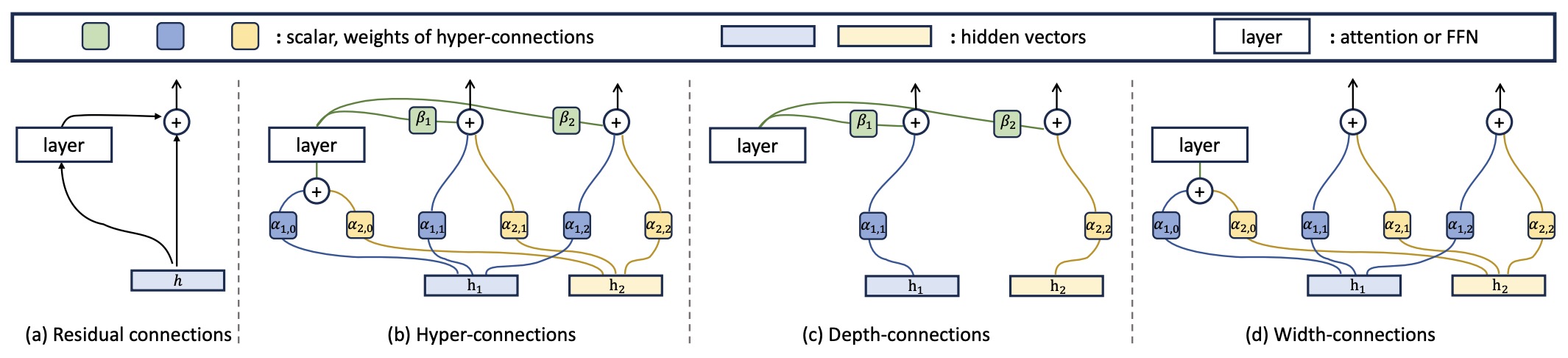
- Together, these three mappings transform residual learning from fixed identity propagation into learned communication across multiple streams.
Dynamic routing
-
An important feature of Hyper-Connections is that the routing matrices are not static. Instead, they depend upon the current hidden representation.
-
For example, the residual mapping is parameterized as:
\[H_l^{\mathrm{res}} = \alpha_l \tanh ( \Theta_l \tilde{X}_l^\top ) + B_l\]-
where:
-
\(\tilde{X}_l\) denotes normalized residual streams,
-
\(\Theta_l\) contains learnable routing parameters,
-
\(B_l\) provides a learned initialization,
-
\(\alpha_l\) controls routing strength.
-
-
-
Consequently, the topology itself becomes input dependent. Different inputs may therefore induce different communication patterns across residual streams. This capability significantly increases the flexibility of the architecture compared with fixed identity mappings.
Relationship to residual learning
-
Classical residual connections emerge as a special case of Hyper-Connections.
-
Suppose \(n=1\), then:
-
The update reduces immediately to \(h_{l+1} = h_l + F(h_l)\) recovering the original ResNet formulation. Hyper-Connections therefore generalize residual learning rather than replacing it.
-
The classical residual block occupies one point within a broader design space of learnable residual topologies.
Advantages
-
Multi-stream residual routing provides several important benefits.
-
Increased communication capacity:
-
Information no longer competes within a single hidden representation.
-
Multiple streams can simultaneously preserve different aspects of the computation.
-
-
Greater representational flexibility:
- Different computational modules may write to different streams, allowing representations to evolve more independently throughout the network.
-
Richer routing patterns:
- Because routing matrices are learned, the model determines how information should propagate rather than relying upon fixed identity shortcuts.
-
Compatibility:
-
Hyper-Connections require no modifications to the internal computations of attention layers or feed-forward networks.
-
Existing Transformer blocks therefore remain unchanged, making the approach broadly compatible with contemporary LLM architectures.
-
Limitations
-
Although Hyper-Connections substantially increase expressive capacity, their flexibility introduces new challenges. Most importantly, the learned residual mixing matrix \(H_l^{\mathrm{res}}\) is unconstrained.
-
Repeated multiplication across many layers yields
\[\prod_i H_i^{\mathrm{res}}\]- whose singular values may either grow or shrink rapidly.
-
Unlike the identity matrix, there is no guarantee that learned routing preserves information or gradient magnitude.
-
Consequently, Hyper-Connections may experience signal amplification, signal attenuation, unstable gradients, optimization instability, and particularly in very deep models.
-
These effects become increasingly severe as the number of residual streams and network depth increase.
Empirical observations
-
The Hyper-Connections paper demonstrates that multi-stream residual routing improves model quality across several Transformer architectures while introducing only modest computational overhead.
-
The learned routing matrices produce richer information flow than fixed identity mappings, and multiple residual streams consistently outperform single-stream baselines across language modeling benchmarks.
-
However, training stability becomes increasingly sensitive at larger model scales, suggesting that unconstrained routing introduces new optimization challenges.
-
This observation motivates the next major development in residual architectures.
Transition to Manifold-Constrained Hyper-Connections
-
Hyper-Connections demonstrate that the residual topology itself can be learned rather than fixed. At the same time, their flexibility reveals an important limitation.
-
The identity shortcut introduced by ResNet possesses remarkable numerical stability because repeated identity mappings neither amplify nor suppress information.
-
Learned routing matrices do not necessarily preserve this property. As a result, the increased expressivity of Hyper-Connections comes at the cost of weaker optimization guarantees.
-
The next section examines Manifold-Constrained Hyper-Connections (mHC), which retain the expressive multi-stream topology introduced by Hyper-Connections while restoring many of the stability properties that originally made residual learning successful. Rather than allowing arbitrary routing matrices, mHC constrains residual mixing to the manifold of doubly stochastic matrices, yielding a residual topology that is simultaneously expressive, learnable, and numerically stable.
Manifold-Constrained Hyper-Connections
-
Hyper-Connections generalize the residual stream by replacing a single fixed identity pathway with multiple interacting residual streams connected through learned routing matrices. This substantially increases the expressive capacity of residual architectures, but it also weakens the most important property that made residual learning successful in the first place: stable identity mapping. In classical residual networks, the shortcut path preserves information exactly. In Hyper-Connections, the shortcut path becomes a learned matrix transformation, and repeated composition of these matrices across depth can amplify, suppress, or distort information unpredictably.
-
mHC: Manifold-Constrained Hyper-Connections by Xie et al. (2025) addresses this problem by constraining the learned residual connection space. Rather than allowing arbitrary residual mixing matrices, mHC projects them onto a structured manifold that preserves identity-like signal propagation while retaining the expressive benefits of multi-stream routing. The result is a residual architecture that is both more flexible than standard residual connections and more stable than unconstrained Hyper-Connections.
-
The central idea is that residual routing should be learnable, but not unconstrained. Just as normalization layers regulate activation scale, manifold constraints regulate residual topology. This allows the model to learn richer communication patterns across residual streams without sacrificing the stability required for large-scale training.
Why unconstrained residual routing becomes unstable
-
In standard residual learning \(x_{l+1} = x_l + F(x_l,W_l)\), expanding across depth yields \(x_L = x_l + \sum_{i=l}^{L-1} F(x_i,W_i)\). The identity term \(x_l\) is preserved exactly, ensuring that information from a shallow layer can reach a deeper layer without modification.
-
Hyper-Connections replace this fixed identity path with learned residual mixing:
- Recursively expanding this recurrence gives a product of residual mappings:
- This product is the source of instability. If the singular values of the residual mappings exceed one, signals grow exponentially. If they fall below one, signals decay. Unlike the identity matrix \(I\), an unconstrained learned matrix does not guarantee stable propagation.
Identity mapping as signal conservation
-
The original residual connection can be interpreted as a conservation law.
-
The shortcut path ensures that the input representation is preserved with coefficient one:
-
This guarantees that neither forward activations nor backward gradients are forced to pass exclusively through learned transformations.
-
In multi-stream residual architectures, the analogous requirement is not that each stream remain fixed independently. Instead, the average signal across streams should remain conserved. A stable residual mapping should redistribute information among streams without arbitrarily increasing or decreasing the total signal.
-
This motivates constraining the residual mapping to behave like a normalized mixing operator.
The mHC constraint
- mHC constrains each residual mixing matrix \(H_l^{\mathrm{res}}\) to lie on the set of doubly stochastic matrices:
-
A doubly stochastic matrix has three defining properties:
-
Every row sums to one.
-
Every column sums to one.
-
Every entry is nonnegative.
-
-
These constraints ensure that the matrix redistributes information among streams rather than arbitrarily amplifying or suppressing it.
-
The following figure (source) shows illustrations of residual connection paradigms, comparing the standard residual connection, unconstrained Hyper-Connections, and Manifold-Constrained Hyper-Connections, where mHC projects residual mapping matrices onto constrained manifolds to improve stability.
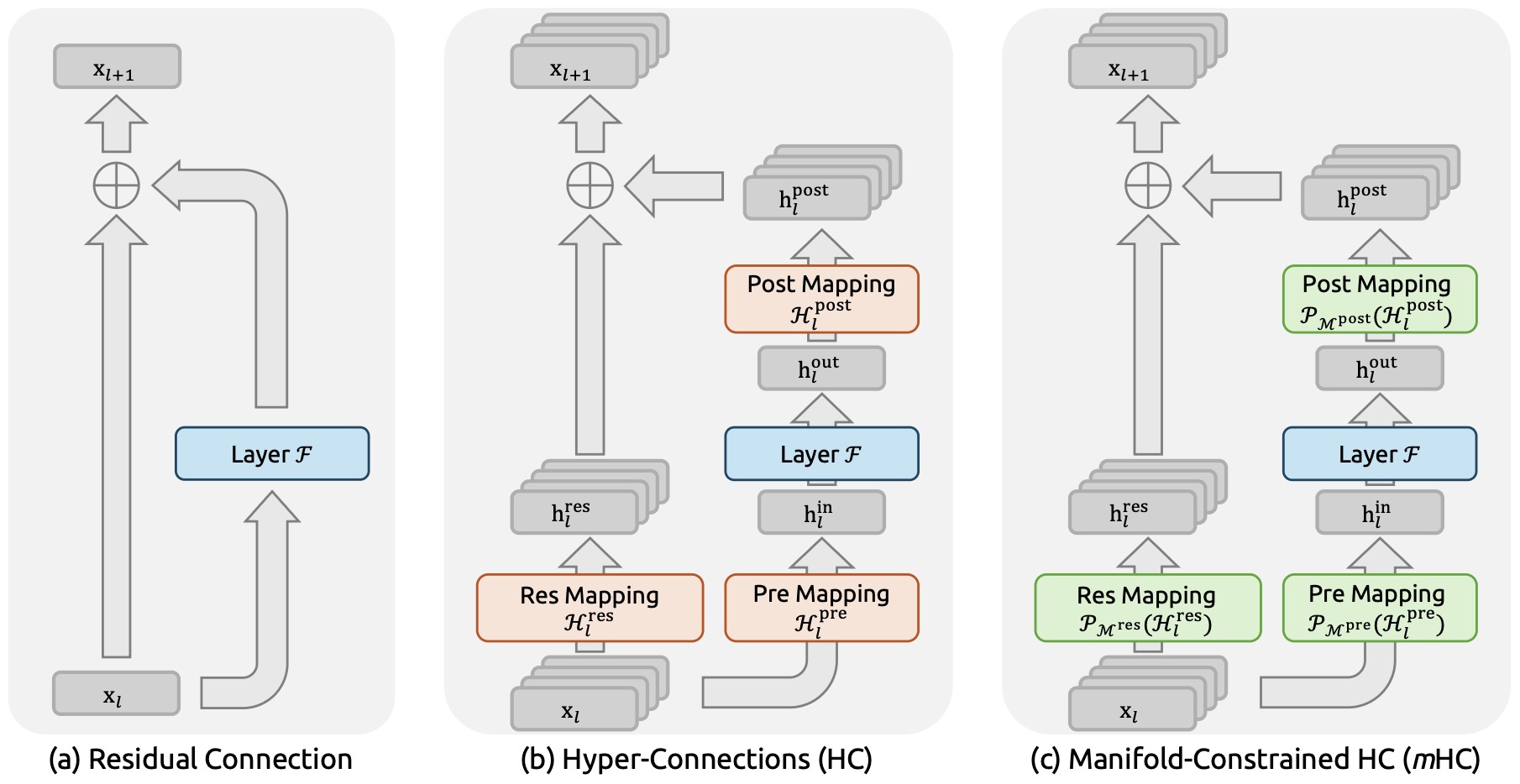
The Birkhoff polytope
-
The set of doubly stochastic matrices is known as the Birkhoff polytope.
-
A fundamental result in matrix theory states that every doubly stochastic matrix can be written as a convex combination of permutation matrices:
-
This interpretation is useful for understanding mHC. A permutation matrix simply rearranges residual streams without changing their magnitudes. A convex combination of permutation matrices therefore performs a softened redistribution of information across streams.
-
Consequently, mHC allows learned stream mixing while preserving the conservation properties associated with identity-like propagation.
Stability properties
- Constraining residual mappings to the Birkhoff polytope provides several important stability guarantees.
Mean preservation
- Because each row and column sums to one \(H\mathbf{1} = \mathbf{1}, \qquad \mathbf{1}^\top H = \mathbf{1}^\top\), this ensures that applying \(H\) does not change the global mean signal across streams.
Nonnegative convex mixing
-
Because \(H_{ij} \ge 0\), each output stream is a convex combination of input streams.
-
The mapping redistributes information rather than extrapolating beyond the span of existing stream values.
Closure under multiplication
-
If \(H_1\) and \(H_2\) are doubly stochastic, then their product \(H_1 H_2\) is also doubly stochastic. This property is essential because deep networks compose residual mappings across many layers.
-
The product \(\prod_i H_i^{\mathrm{res}}\) therefore remains within the same stable manifold.
Identity-like propagation
- Although mHC does not require every residual mapping to equal the identity matrix, it preserves the key property that made identity mappings useful: stable signal propagation across arbitrary depth.
Parameterization and projection
-
mHC begins with the same dynamic mapping structure used in Hyper-Connections.
-
A residual mapping is first computed as an unconstrained matrix,
- This matrix is then projected onto the manifold:
- The projection operator ensures that the final matrix satisfies the doubly stochastic constraints.
Sinkhorn-Knopp projection
-
mHC uses the Sinkhorn-Knopp algorithm to perform the projection.
-
Concerning nonnegative matrices and doubly stochastic matrices by Sinkhorn and Knopp (1967) introduced an iterative matrix-scaling procedure that alternates between row normalization and column normalization until the matrix becomes approximately doubly stochastic.
-
At a high level, the procedure repeats \(H \leftarrow \frac{H}{H\mathbf{1}}\) followed by \(H \leftarrow \frac{H}{\mathbf{1}^\top H}\). In practice, implementations use numerically stable variants, often operating in log space or with entropic regularization.
-
Because the procedure is differentiable, gradients can propagate through the projection step during backpropagation.
Manifold constraints beyond the residual mapping
-
Although the residual mapping is the most important component for stability, mHC also constrains other connection matrices.
-
The full architecture contains:
-
a pre-mapping that reads from multiple streams,
-
a post-mapping that writes updates back to streams,
-
a residual mapping that mixes streams across depth.
-
-
Each of these mappings has a corresponding constrained space.
-
The residual mapping receives the strongest constraint because it composes repeatedly across depth and therefore has the greatest influence on stability.
Systems efficiency
- mHC introduces additional overhead because it widens the residual stream from \(d\) to \(n \times d\), and performs additional routing computations. Naïvely implemented, this could significantly increase memory access cost. The paper therefore incorporates several systems optimizations.
Kernel fusion
-
Multiple routing operations are fused into custom GPU kernels to reduce memory traffic.
-
Because modern accelerators are often limited by memory bandwidth rather than arithmetic throughput, reducing reads and writes can substantially improve wall-clock efficiency.
Mixed precision kernels
- mHC employs mixed precision implementations to reduce bandwidth requirements while maintaining numerical stability.
Selective recomputation
- Rather than storing every intermediate routing activation, selected quantities are recomputed during the backward pass. This reduces activation memory at the cost of modest additional computation.
Communication overlap
- Distributed training schedules overlap communication with computation, reducing pipeline stalls. This is particularly important because widened residual streams increase inter-device communication requirements.
Empirical behavior
-
The paper reports that unconstrained Hyper-Connections can experience severe instability during large-scale training, including loss spikes and abnormal gradient behavior.
-
The following figure (source) shows training instability in Hyper-Connections, comparing the absolute loss gap and gradient norm behavior of HC and mHC in 27B-parameter model training.
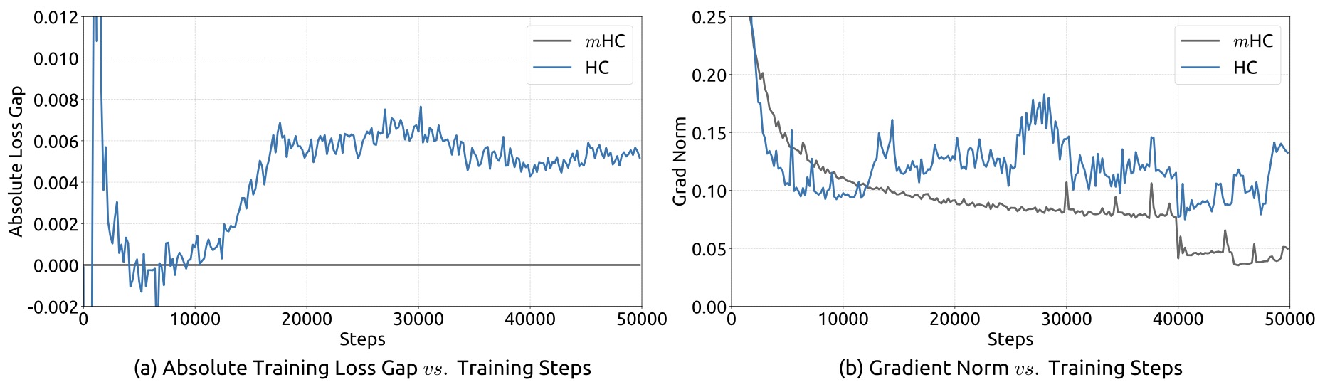
-
mHC stabilizes these dynamics by constraining residual routing while retaining the benefits of expanded residual topology.
-
The following figure (source) shows propagation instability in Hyper-Connections, including single-layer and composite residual mapping gain magnitudes for forward signals and backward gradients in a 27B-parameter model.
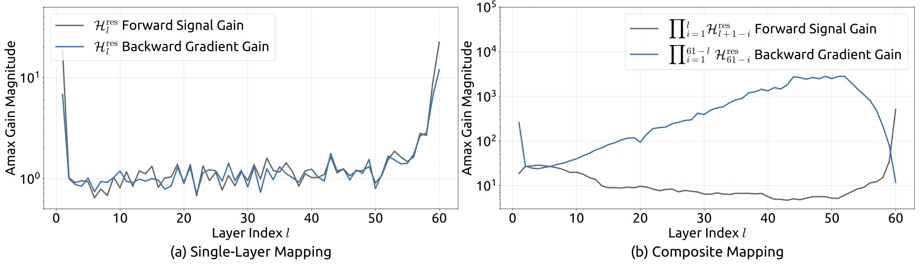
- Empirically, mHC demonstrates: improved training stability, better scalability at large model sizes, stronger downstream performance than unconstrained Hyper-Connections, and modest additional training overhead when implemented with optimized kernels.
Relationship to standard residual connections
-
mHC can be understood as a strict generalization of standard residual learning.
-
When \(n=1\), the doubly stochastic constraint reduces to \(H=[1]\) and the architecture collapses to the classical residual update:
- Thus, standard residual connections are a special case of mHC. This relationship is conceptually important because it shows that mHC does not discard the residual learning principle. Instead, it extends identity mappings into a broader class of stable multi-stream transformations.
Relationship to Attention Residuals
-
Attention Residuals and mHC address complementary limitations of standard residual streams: Attention Residuals modify how information is selected across depth, while mHC modifies how information is routed across residual streams.
-
The two mechanisms therefore operate along different axes:
-
Attention Residuals introduce adaptivity over layer history.
-
mHC introduces adaptivity over residual stream topology.
-
-
This distinction suggests that future architectures may combine both ideas, using attention to retrieve useful historical representations while using constrained multi-stream routing to preserve and transform them stably.
Interpretation
-
Manifold-Constrained Hyper-Connections introduce an important design principle for future neural architectures: learned connectivity should be expressive, but geometrically constrained.
-
Unconstrained flexibility often improves representational power in small-scale experiments but becomes unstable at scale.
-
By restricting residual routing to a well-conditioned manifold, mHC demonstrates that architectural expressivity and optimization stability need not be opposing goals.
-
Instead, the residual connection can be treated as a structured object whose geometry is designed explicitly to preserve stable signal propagation.
Transition to comparative design guidance
-
At this point, the primer has traced the evolution of skip connections from simple identity shortcuts to adaptive, learnable, and geometrically constrained residual pathways.
-
The next section synthesizes these ideas into a comparative design framework, explaining when each type of skip or residual connection is most appropriate, what problem it solves, and what tradeoffs it introduces.
Comparative Design Guidance
-
The preceding chapters have traced the evolution of skip and residual connections from their origins in early deep neural networks to the sophisticated routing mechanisms employed by modern Transformer architectures. Although these architectures differ considerably in implementation, they all address a common challenge: preserving useful information as computation progresses through increasingly deep networks. The principal differences lie in what information they preserve, how that information is propagated, and whether the communication pattern remains fixed or is learned during training.
-
This progression illustrates that skip connections have evolved from simple optimization aids into fundamental communication mechanisms. Early architectures focused primarily on ensuring stable gradient propagation. Subsequent work emphasized feature reuse, spatial information preservation, adaptive depth-wise retrieval, and learnable residual topologies. Modern residual architectures increasingly treat connectivity itself as a first-class design problem, recognizing that how information flows through a network is often as important as the computations performed within individual layers.
-
This section summarizes the major architectural paradigms discussed throughout the primer, highlighting their respective strengths, limitations, and appropriate application domains.
Evolution of design objectives
-
The historical progression of skip connections can be viewed as a gradual expansion of architectural objectives:
-
The earliest architectures sought to improve optimization. Residual Networks demonstrated that identity mappings dramatically reduce optimization difficulty by allowing layers to learn incremental refinements rather than complete transformations. DenseNet shifted the focus toward feature reuse, showing that preserving intermediate representations explicitly can improve parameter efficiency while reducing redundant computation. U-Net extended skip connections across changes in spatial resolution, enabling encoder-decoder architectures to preserve fine-grained spatial detail during image reconstruction.
-
Transformers reinterpreted residual connections as persistent computational streams shared by every module in the network. Rather than serving merely as optimization shortcuts, residual streams became the primary medium through which information is exchanged across depth.
-
Recent architectures further generalize this idea. Attention Residuals make residual aggregation adaptive by allowing layers to retrieve useful historical representations selectively. Hyper-Connections increase communication capacity by introducing multiple interacting residual streams. Manifold-Constrained Hyper-Connections retain this increased expressivity while imposing geometric constraints that preserve stable signal propagation.
-
-
Taken together, these developments demonstrate a consistent trend toward increasingly adaptive information routing without sacrificing optimization stability.
Comparison of skip and residual connection paradigms
- The following table summarizes the principal architectural differences among the major skip connection mechanisms discussed throughout this primer.
| Architecture | Skip mechanism | Primary objective | Information preserved | Learnable routing | Typical applications |
|---|---|---|---|---|---|
| Plain networks | None | Sequential feature extraction | None | No | Early deep networks |
| Highway Networks | Gated interpolation | Optimization | Hidden representation | Yes | Early deep architectures |
| ResNet | Identity addition | Stable optimization | Residual representation | No | CNNs, Transformers |
| DenseNet | Dense concatenation | Feature reuse | Intermediate feature maps | No | Image classification |
| U-Net | Long-range concatenation | Spatial preservation | High-resolution encoder features | No | Segmentation, diffusion models |
| Transformer residual stream | Identity addition | Persistent computation | Shared hidden representation | No | Large language models |
| Attention Residuals | Depth-wise attention | Adaptive retrieval across depth | Previous layer representations | Yes | Deep Transformers |
| Hyper-Connections | Multi-stream routing | Increased communication capacity | Multiple residual streams | Yes | Transformer architectures |
| Manifold-Constrained Hyper-Connections | Constrained multi-stream routing | Stable adaptive routing | Structured residual topology | Yes | Large-scale Transformers |
- Although these architectures appear quite different, they can be viewed as occupying different points within a common design space whose principal dimensions are information preservation, routing flexibility, and optimization stability.
Fixed versus adaptive connectivity
-
One useful way to categorize skip connections is according to whether their communication topology is fixed or learned.
-
Fixed connectivity:
-
Classical architectures employ predetermined connectivity patterns established during model design.
-
Examples include: ResNet identity shortcuts, DenseNet dense concatenation, U-Net encoder-decoder skip connections, and standard Transformer residual streams.
-
These architectures provide highly predictable optimization behavior while introducing relatively little computational overhead. However, every input follows the same communication pattern regardless of its complexity or semantic content.
-
-
Adaptive connectivity:
-
Recent architectures instead learn how information should propagate. Examples include: Highway Networks, Attention Residuals, Hyper-Connections, and Manifold-Constrained Hyper-Connections.
-
Rather than assuming that all information should flow uniformly, adaptive connectivity allows the model to determine which previous layers should contribute, which residual streams should interact, how information should be redistributed, and how routing should change across inputs. This increased flexibility generally improves representational capacity but introduces additional optimization and systems complexity.
-
Addition versus concatenation
-
Another useful distinction concerns how multiple representations are combined.
-
Additive connections:
-
Additive skip connections preserve constant hidden dimensionality. The general form is \(h_{l+1} = h_l + \Delta_l\).
-
Advantages include: constant representation size, efficient memory usage, direct identity pathways, and straightforward optimization.
-
These properties explain why additive residual learning dominates modern Transformer architectures.
-
-
Concatenative connections:
-
Concatenative skip connections preserve every feature independently.
-
The general form is \(h_{l+1} = [h_1; h_2; \cdots]\).
-
Advantages include: explicit feature preservation, extensive feature reuse, and no destructive merging of representations.
-
Their primary disadvantage is increasing dimensionality, which leads to higher memory consumption and computational cost.
-
Single-stream versus multi-stream architectures
-
Modern residual architectures can also be categorized according to the number of persistent residual representations maintained throughout the network.
-
Single residual stream:
-
Classical residual learning maintains one evolving hidden representation \(h_l\).
-
Every computational module reads from and writes to this shared representation. This design is computationally efficient and has proven remarkably successful for modern LLMs. However, all information must coexist within the same representational space.
-
-
Multi-stream residual architectures:
-
Hyper-Connections and mHC instead maintain \(n\) parallel residual streams, \(X_l \in \mathbb{R}^{n\times d}\). This increases communication capacity by allowing different computations to evolve more independently.
-
The tradeoff is increased memory usage, routing complexity, and implementation overhead.
-
Static versus dynamic aggregation
-
Residual architectures also differ according to how previous information is aggregated.
-
Static aggregation:
-
ResNet computes \(h_l = h_{l-1} + f_{l-1}(h_{l-1})\), implicitly assigning equal weight to every residual update.
-
The aggregation rule remains fixed throughout training.
-
-
Dynamic aggregation:
-
Attention Residuals instead compute
\[h_l = \sum_i \alpha_i v_i\]- where \(\alpha_i\) depends upon the current layer.
-
The residual stream therefore becomes a learned retrieval mechanism rather than a fixed accumulation.
-
This distinction mirrors the transition from fixed convolution kernels to adaptive self-attention in sequence modeling.
-
Optimization and systems tradeoffs
-
As residual architectures become more expressive, they also become more expensive. Several recurring tradeoffs emerge.
-
Expressivity versus stability:
- Greater routing flexibility generally increases representational capacity. However, unconstrained routing can destabilize optimization. This motivates constrained formulations such as mHC.
-
Feature preservation versus memory:
- Concatenative architectures preserve more information explicitly. However, they require substantially more activation memory. Residual addition sacrifices some explicit feature preservation in exchange for constant hidden dimensionality.
-
Adaptivity versus efficiency:
-
Adaptive routing mechanisms improve information utilization. However, they require additional attention computations, routing parameters, and communication.
-
Practical architectures therefore balance representational gains against systems cost.
-
-
Communication versus computation:
-
Large-scale Transformer training is increasingly limited by communication rather than arithmetic throughput. Recent residual architectures explicitly account for this reality.
-
For example, Block Attention Residuals reduce inter-device communication through hierarchical depth aggregation, while mHC introduces kernel fusion and communication overlap to mitigate the cost of multi-stream routing.
-
These considerations illustrate that modern architectural design increasingly depends upon hardware-aware optimization.
-
Design guidelines
-
The choice of skip or residual connection depends primarily upon the computational requirements of the task:
-
Standard residual connections remain the preferred choice when optimization stability, computational efficiency, and architectural simplicity are the primary objectives.
-
Dense connectivity is well suited to problems where extensive feature reuse improves parameter efficiency and model performance.
-
Long encoder-decoder skip connections are most appropriate when preserving high-resolution spatial information is essential.
-
Transformer residual streams provide an effective shared computational substrate for sequential reasoning and autoregressive language modeling.
-
Attention Residuals are most beneficial when extremely deep Transformers require adaptive retrieval of historical layer representations.
-
Hyper-Connections increase residual communication capacity by allowing multiple interacting residual streams, making them attractive for architectures that benefit from richer internal routing.
-
Manifold-Constrained Hyper-Connections are appropriate when multi-stream routing is desired without sacrificing optimization stability during large-scale training.
-
-
No single architecture dominates across every application. Rather, each reflects a different balance among optimization, information preservation, representational flexibility, computational efficiency, and systems scalability.
Future directions
-
Recent research suggests that skip and residual connections remain an active area of architectural innovation despite their long history. Several promising directions are emerging:
-
Learned routing policies that jointly optimize communication across sequence positions, network depth, and residual streams.
-
Architectures that combine depth-wise attention with multi-stream residual routing, integrating ideas from Attention Residuals and Hyper-Connections.
-
Hardware-aware residual mechanisms that optimize communication patterns for increasingly distributed accelerator clusters.
-
Adaptive residual topologies that evolve dynamically throughout training rather than remaining fixed after initialization.
-
Theoretical analyses that characterize residual routing in terms of optimization geometry, information theory, and dynamical systems.
-
-
As frontier models continue to scale, these questions are likely to become increasingly important. The evolution described throughout this primer suggests that future advances in deep learning will depend not only on improving the computations performed within individual layers, but also on designing increasingly effective mechanisms for communicating information between them.
References
Foundational residual connections and identity mapping
- Learning representations by back-propagating errors by Rumelhart et al. (1986)
- Deep Residual Learning for Image Recognition by He et al. (2015)
- Identity Mappings in Deep Residual Networks by He et al. (2016)
- Highway Networks by Srivastava et al. (2015)
- Densely Connected Convolutional Networks by Huang et al. (2017)
- FractalNet: Ultra-Deep Neural Networks without Residuals by Larsson et al. (2016)
Skip connections in segmentation and biomedical vision
- U-Net: Convolutional Networks for Biomedical Image Segmentation by Ronneberger et al. (2015)
- 3D U-Net: Learning Dense Volumetric Segmentation from Sparse Annotation by Çiçek et al. (2016)
- The Importance of Skip Connections in Biomedical Image Segmentation by Drozdzal et al. (2016)
Transformer architectures and normalization
- Attention Is All You Need by Vaswani et al. (2017)
- Language Models are Few-Shot Learners by Brown et al. (2020)
- LLaMA: Open and Efficient Foundation Language Models by Touvron et al. (2023)
- Root Mean Square Layer Normalization by Zhang and Sennrich (2019)
Attention Residuals and depth-wise aggregation
- Attention Residuals by Kimi Team et al. (2026)
- A Survey of Attention Mechanisms in Deep Learning by Chaudhari et al. (2019)
Hyper-Connections and residual stream generalization
- Hyper-Connections by Zhu et al. (2024)
Manifold-Constrained Hyper-Connections and stability
- mHC: Manifold-Constrained Hyper-Connections by Xie et al. (2025)
- Concerning nonnegative matrices and doubly stochastic matrices by Sinkhorn and Knopp (1967)
Optimization, scaling, and efficiency
- Visualizing the Loss Landscape of Neural Nets by Li et al. (2018)
- Efficient Memory Management for Large Language Model Serving with PagedAttention by Kwon et al. (2023)
- FlashAttention: Fast and Memory-Efficient Exact Attention by Dao et al. (2022)
- Training Compute-Optimal Large Language Models by Hoffmann et al. (2022)
Books, blogs, explainers, and ecosystem discussions
- Neural Networks and Deep Learning by Nielsen (2018)
- The Annotated Transformer
- Feature Visualization by Olah et al. (2017)
Citation
If you found our work useful, please cite it as:
@article{Chadha2020DistilledSkipConnections,
  title   = {Skip/Residual Connections},
  author  = {Chadha, Aman},
  journal = {Distilled AI},
  year    = {2020},
  note    = {\url{https://aman.ai}}
}