CS231n • Visualizing and Understanding
- Review: Computer Vision Tasks
- Under the hood of a ConvNet
- Visual viewpoint of the linear classifier
- Visualizing the first layer
- Visualizing weights at higher layers
- Visualizing internal representations/activations
- Patch-level maximal activation analysis
- Which pixels matter: Saliency via Occlusion
- Which pixels matter: Saliency via Backprop
- Saliency maps + GrabCut: Segmentation without supervision
- Saliency maps: Uncover biases
- Guided Backprop
- Gradient Ascent
- Deep Generator Network (almost a GAN but not quite!)
- Fooling Images / Adversarial Examples
- DeepDream: Amplify existing features
- What is a CNN learning: Earlier layers vs. later layers
- Feature Inversion
- Texture Synthesis
- Neural Style Transfer: Feature Inversion + Gram Matrices
- Key Takeaways
- Further Reading
- Citation
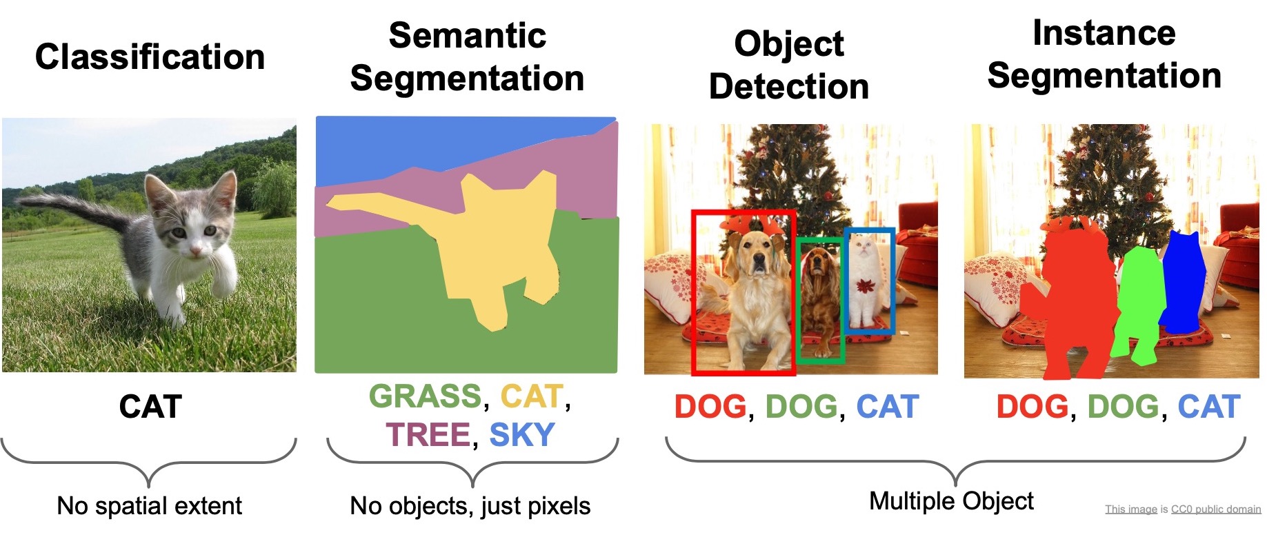
Review: Computer Vision Tasks
- We’ve talked about architectural design in the context of convolutional neural networks. We’ve primarily studied this within the purview of image classification.
- In the last couple of topics, we’ve been looking at the other tasks outside of classification, specially, we took a look at generative approaches where we attempt to generate images. We studied this in the context of VAEs and GANs.
- In “Detection and Segmentation”, we also talked about semantic segmentation, object detection and instance segmentation. We talked about specific architectures that have been really popular such as R-CNN, Fast R-CNN, Faster R-CNN, Mask R-CNN, YOLO, SSD etc.
- The problems of image classification, semantic segmentation, object detection and instance segmentation are the core computer vision problems that are the focus of researchers and being worked on heavily as of today. Looking at popular computer vision conferences in the last couple of years, a majority of the papers tackle some form or the other of these types of tasks, related to detection or segmentation. These problems are this considered unsolved in the field since they fail to generalize efficiently to the real world under certain scenarios and only work under a specific subset of cases. Lots of work to be done here!
Under the hood of a ConvNet
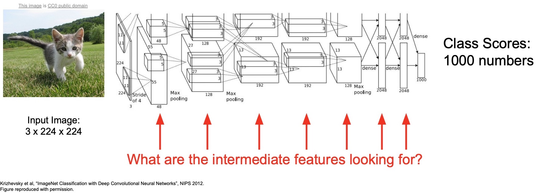
- So far, we’ve been treating this ConvNets as large black boxes. Inputs come in as pixels, transformations are applied on the pixels and out comes class scores that help perform classification.
- We’ve been talking about how to interpret these transformations in terms of a visual interpretation, geometric interpretation and an analytical interpretation. But, we’ve largely been treating them as just black boxes that generate a set of scores at the output.
- A common criticism with neural networks, especially when we’re seeking to deploy them for real world use-cases is that its not really easy to interpret their internals.
- The problem is that when these models make mistakes after deployment, it’s really hard to explain why the model failed. Not just that, figuring out how we can go about improving the model, is another burning question that warrants an answer.
- We’ll be specifically diving into what exactly is a ConvNet learning, what are the features in every layer, how do we go about interpreting these features, how do we think about what the neurons are doing, what are the activations that are being produced at every single layer?
- Next, we’ll be thinking about ways to visualize/interpret the results that we obtain as outputs from our ConvNets.
Visual viewpoint of the linear classifier
- We’ve covered the visual interpretation of what your linear classifier is learning in the topic on image classification.
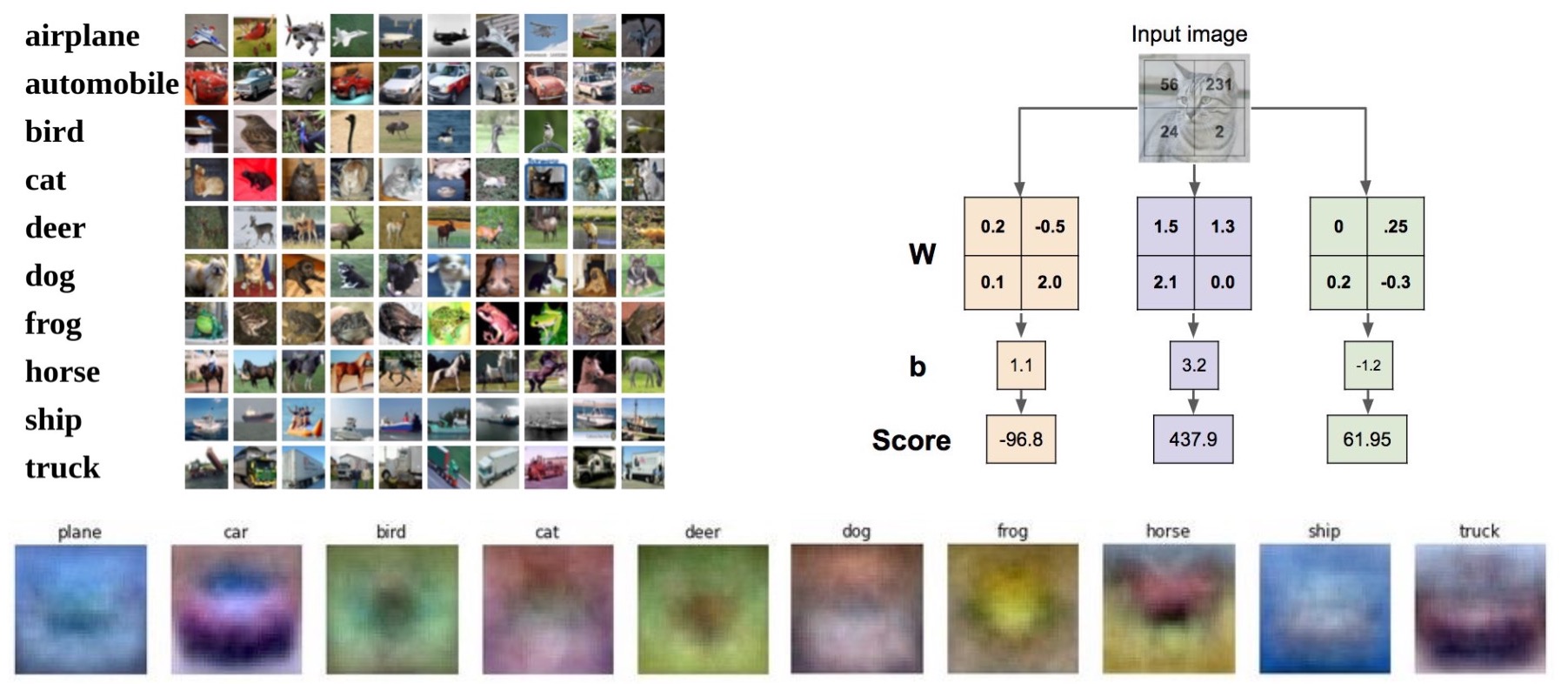
- Specifically studied this in the context of CIFAR-10 (with ten classes, hence called CIFAR-10) and each row of your weight matrix can be stretched back out into an image that represents generally what that class is really learning to represent.
- Recall that in a linear classifier, each row essentially represents a template of a particular class. Here, we’re taking that row and re-shaping it back into the size of the input image which is \(32 \times 32 \times 3\), and we’re visualizing what that would look like if it were an image.
- Earlier, we talked about how some of these are kind of interpretable, note the car class, plane class, ship class and the (double-headed) horse class. For instance, the plane and ship class looks really blue because they are representing the sky or the ocean respectively. The car more or less looks like an actual front facing car. The horse looks like a double-headed horse, one looking to the left, one looking to the right because both kinds of images probably exist in the dataset.
- Linear classifiers are thus relatively easy to interpret. But that can’t necessarily be said for ConvNets because you can’t reshape the weights that you learnt into the size of an image having 3 input dimensions because often times the channels that we have in the intermediate layers are much larger than 3 (and depend on the number of filters used on the activation volume of the prior layer to produce activations for the next layer).
Visualizing the first layer
- Since directly inspecting the weights isn’t possible with ConvNets, we can still visualize the very first layer of our ConvNet because that takes in the input image and transforms it, so we can reshape those weights back and see what they look like.
- The figure below visualizes the very first Conv layers of AlexNet, ResNet-18/101, DenseNet-121 and we’re taking a lot at what the weights in the very first layer are learning. In AlexNet, you have \(11 \times 11\) convolutions and so each of these blocks represent a \(11 \times 11\) image that’s learnt by the weights of the convolution block. Because AlexNet has \(64\) of these, we’re visualizing 64. Infact, all of them have \(64\) but the later models, ResNet18/101 don’t use \(11 \times 11\) filters but instead use \(7 \times 7\) so those images are a little smaller.
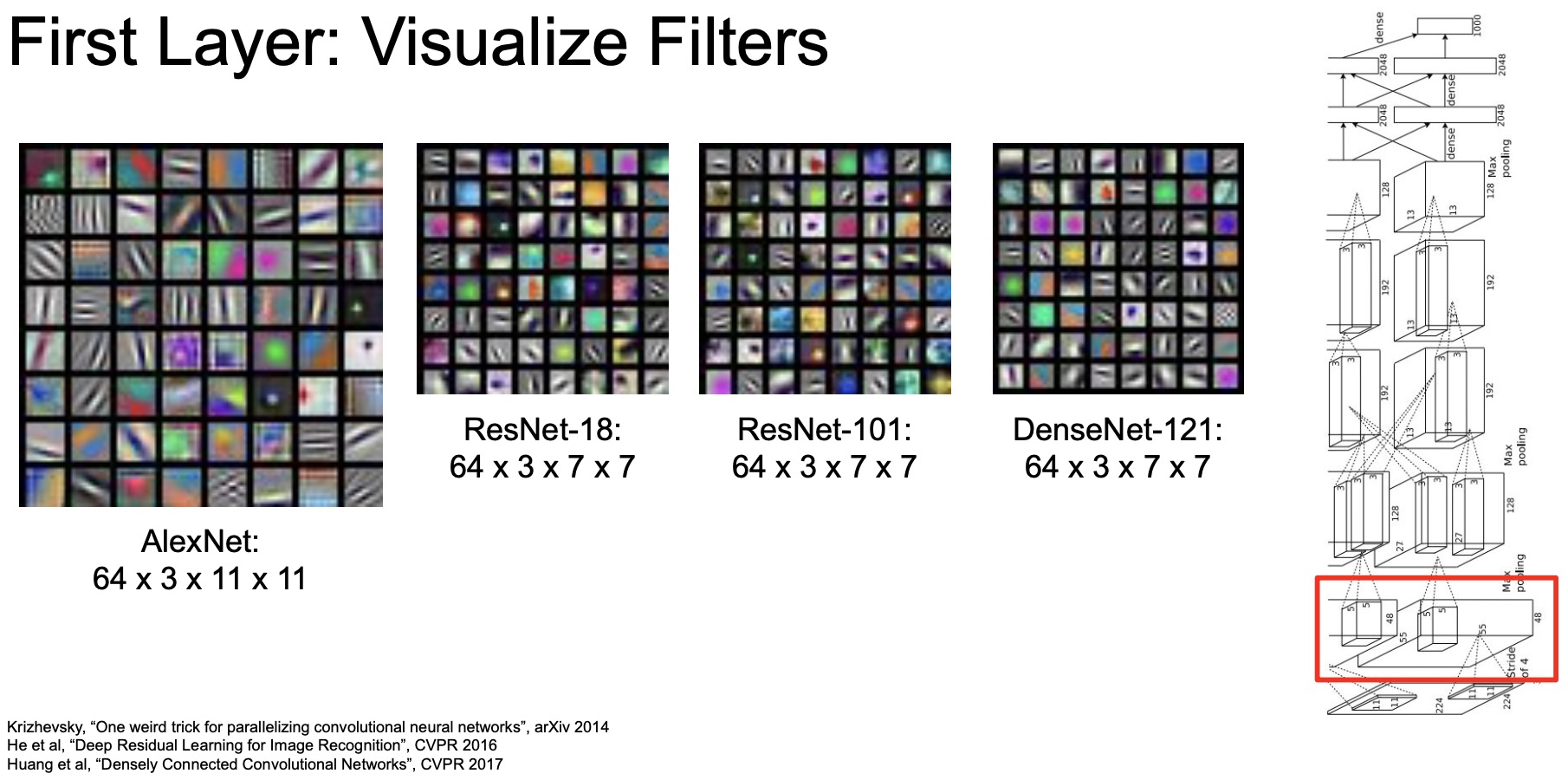
As shown in the illustration above, the filters in first layer are learning primitive shapes, oriented edges, blob-like structures and opposing colors, just like the human brain does.
- For e.g., at the top left of the image above, you see that AlexNet has learned something that looks like a green blob surrounded by a purple hue. These oriented edges and blob-like structures are consistent with the models that Hubel and Wiesel found in their seminal work that won the Nobel Prize in 1960 when they injected electrodes into a cat’s visual system and tried to measure what kind of stimuli those neurons were reacting to. They found that cats neurons in the first visual layer were also reacting to these oriented edges and blob-like structures.
- The convolutional neural networks that we’re training are also learning similar representations as well. And note that it’s consistent across all of these different kinds of architectures.
Infact, these filters look mostly similar on popular deep ConvNets, for e.g., AlexNet, VGG, GoogleNet, or ResNet.
Visualizing weights at higher layers
- We can’t necessarily visualize filters from higher layers because they don’t usually have a channel depth of 3. Considering the example of AlexNet, which transforms the input image into an activation with a \(64\) dimensional channel width at the next layer, which is hard to reshape. But what we could do instead is treat each channel as an individual set of weights and then visualize them individually.
- Yosinski et al. presented a study of what that looks like. In the diagram below, at the very top, we’re looking at the very first few layers that we visualized earlier where we see the edges and the blobs.
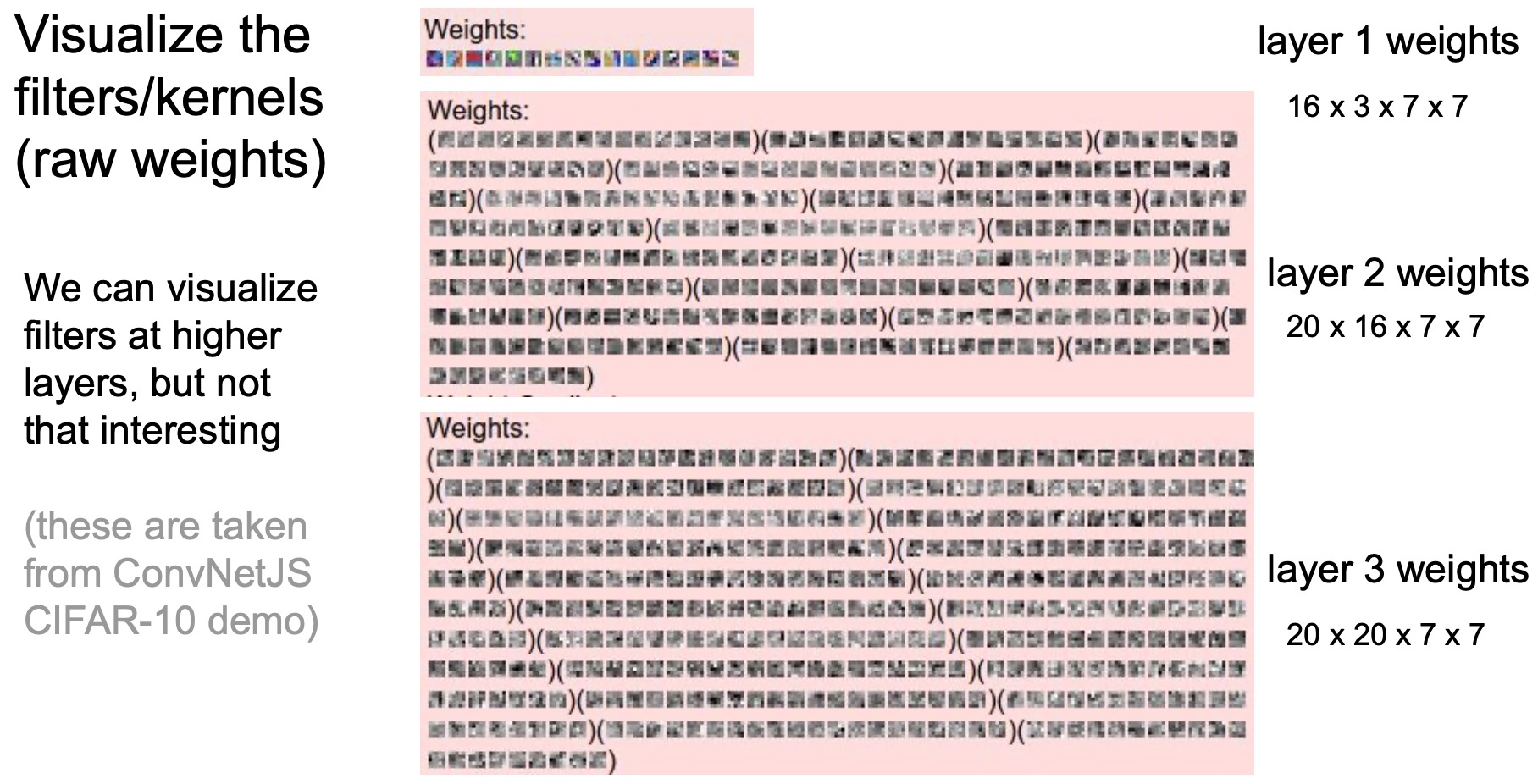
- Next, we visualize the weights of the second layer which are \(7 \times 7\) grayscale images and there’s \(20 \times 16\) of them because 16 is the input dimension and \(20\) is the output dimension. Note that this is for a custom architecture (not AlexNet) which was built for demonstration purposes.
- This is actually the model running on the course website right now.
If you look at the weights of the second or the third layer, we can’t really interpret these results anymore. While it was nice that we could interpret the very first layer’s weights, anything beyond the first layer is really hard to make sense of. Alone they don’t make as much sense unless they’re put together along all the channels.
- We need to develop newer ways of interpreting what these intermediate layers are actually learning and that’s where comes our very first interpretation algorithm.
- Here we are only primarily interested in understanding what is learned by the very last layer of our convolutional neural networks. In other words, the feature vectors that we’ll be interacting with, thus, are the last-layer representations learned by the convolutional neural network model (in this case, AlexNet), pre-trained on ImageNet, for every single image.
- We begin our journey at the very last layer and we’ll make our way into some of the more intermediate layers in the later sections.
- The reason we want to start with the last layer is because this last layer is often used to train other downstream tasks. For e.g., when we talked about image captioning, we took a pre-trained convolutional neural network, extracted the last layer features and then use that as input to a recurrent neural net or a transformer, so this last layer must capture something that’s meaningful about the image.
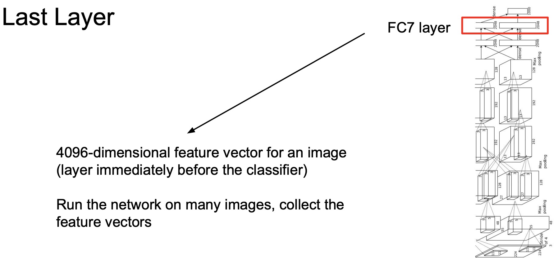
- Let’s start off with thinking about the ways to build our understanding around what’s in this 4096-D vector obtained from the last fully-connected (FC) layer in AlexNet.
- The way we’re gonna do this is we’re gonna take a bunch of images, feed it through our network and represent each image as a 4096-D vector. Next, we’re going to apply nearest neighbors to figure out which images in the training set match the most with the test image. Earlier, we applied nearest neighbors in the pixel space (shown below) to a test image, and pulled out all the nearest neighbors from the training set to perform classification using majority vote. Now, we’ll be applying nearest neighbors not in pixel space, but in this 4096-D vector representation of all of our images.
- When performing nearest neighbors in pixel space, you’ll notice that there are a lot of errors that this model makes.
- Specifically, if you look at the very first image it looks like it’s a boat that’s moving towards the top right, but the nearest neighbors algorithm is picking up a bird that’s looking to the top right and a horse that’s looking to the right. This is because they have the same sort of pixel gradients moving towards the top right.
- Even the second image which looks like a white dog, but a lot of its nearest neighbors are being picked up as other kinds of round blobby structures like cats and other animals.
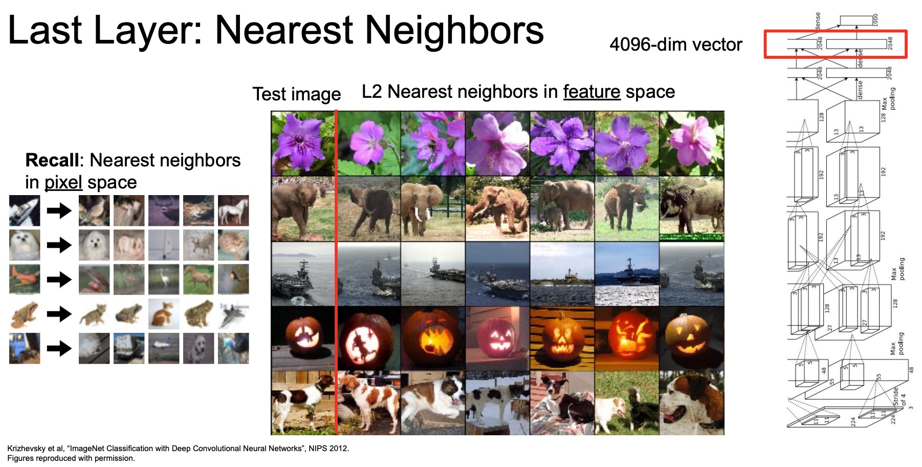
- So, this nearest neighbor approach in pixel space doesn’t always work out very well owing to it solely relying on pixel gradients as its only means of input.
- Let’s see what happens if we run this instead on 4096-D vector that we extract from our images using the convolutional neural network.
- Here’s some examples of nearest neighbors using the 4096-D, a high dimensional vector. If you notice, these look a lot better and seem to be capturing more than just pixel information, rather they seem to be capturing a lot of semantic information.
- The reason it’s capturing the semantic information can be inferred by looking at some of these examples. Looking at the elephant that’s looking to the right, this particular elephant and any of its nearest neighbors don’t really show a significant commonality in the pixel space, i.e., they don’t share a lot of “similar” (RGB intensity) pixels in the same location, but they’re still sort of picked up as being its nearest neighbors. Looking deeper, while the test elephant image in question has a right-faced elephant, some of the elephants that are returned are looking to the left, some are looking directly at the camera, some are running in a different direction and yet the model is still able to take all of these different poses and orientations, and decompose them into a vector representation in this high dimensional space such that all the elephants “live” close together in this space.
- This is an indication that the model is capturing some amount of semantics within these images that goes beyond just what’s available in the pixel.
- Note that the way we’re measuring nearest neighbors here is using L2 distance between any two 4096-D vectors corresponding to two images.
- In fact, this is not just true for the elephant class, this is also similar for the dog class the dogs are also in various different poses and orientations and still they’re being pulled out as its nearest neighbors.
- Next, lets try visualizing all of these 4096-D images in a 2D reduction projected space. To reduce a 4096-D vector into a 2D space, we can deploy a variety of different algorithms.
PCA
- Principal Component Analysis (PCA) is a linear feature extraction technique invented in 1901 by Karl Pearson that uses orthogonal transformations to map a set of variables into a set of linearly uncorrelated variables called Principal Components.
- PCA performs a linear mapping of the data to a lower-dimensional space in such a way that the variance of the data in the low-dimensional representation is maximized.
- It does so by calculating the eigenvectors from the covariance matrix. The eigenvectors that correspond to the largest eigenvalues (the principal components) are used to reconstruct a significant fraction of the variance of the original data.
- In simpler terms, PCA combines your input features in such a way that you can drop the least important features, while still retaining the most valuable parts of all of the features.
- As a result, each of the new features or components created after PCA are all independent of one another.
- Read more on the implementation details of PCA in Coursera-NLP | Word Embeddings and Vector Spaces.
- (-) PCA as a dimensionality reduction method is simple but not as effective. There are more powerful methods than PCA that people typically use for deep learning models.
t-SNE
- t-distributed Stochastic Neighbor Embedding (t-SNE) is another visualization method.
- (+) It is a non-linear technique for dimensionality reduction that is particularly well suited for the visualization of high-dimensional datasets. It is extensively applied in image processing, NLP, genomic data and speech processing.
- The technique takes a population of these large high dimensional vectors and projects them down into a lower dimensional space. The end goal of this technique is that similar points in this high dimensional space are still close together in two dimension in space and they’re further away if they’re also further away in the high dimensional space.
- Here’s a brief overview of the inner workings of t-SNE:
- The algorithms starts by calculating the probability of similarity of points in high-dimensional space and calculating the probability of similarity of points in the corresponding low-dimensional space. The similarity of points is calculated as the conditional probability that a point A would choose point B as its neighbor if neighbors were picked in proportion to their probability density under a Gaussian (normal distribution) centered at A.
- It then tries to minimize the difference between these conditional probabilities (or similarities) in higher-dimensional and lower-dimensional space for a perfect representation of data points in lower-dimensional space.
- To measure the minimization of the sum of difference of conditional probability t-SNE minimizes the sum of Kullback-Leibler divergence of overall data points using a gradient descent method.
- Note that Kullback-Leibler divergence or KL divergence is is a measure of how one probability distribution diverges from a second, expected probability distribution. For the curious reader interested in knowing the detailed working of t-SNE, refer to “Visualizing Data using t-SNE” (2008) by Maaten and Hinton.
- In simpler terms, t-Distributed stochastic neighbor embedding (t-SNE) minimizes the divergence between two distributions: a distribution that measures pairwise similarities of the input objects and a distribution that measures pairwise similarities of the corresponding low-dimensional points in the embedding.
- In this way, t-SNE maps the multi-dimensional data to a lower dimensional space and attempts to find patterns in the data by identifying observed clusters based on similarity of data points with multiple features. However, after this process, the input features are no longer identifiable, and you cannot make any inference based only on the output of t-SNE. Hence it is mainly a data exploration and visualization technique.
- An example of some nice big data visualizations can be found here. How to Use t-SNE Effectively explores how t-SNE behaves in simple cases, and helps develop an intuition for what’s going on under-the-hood.
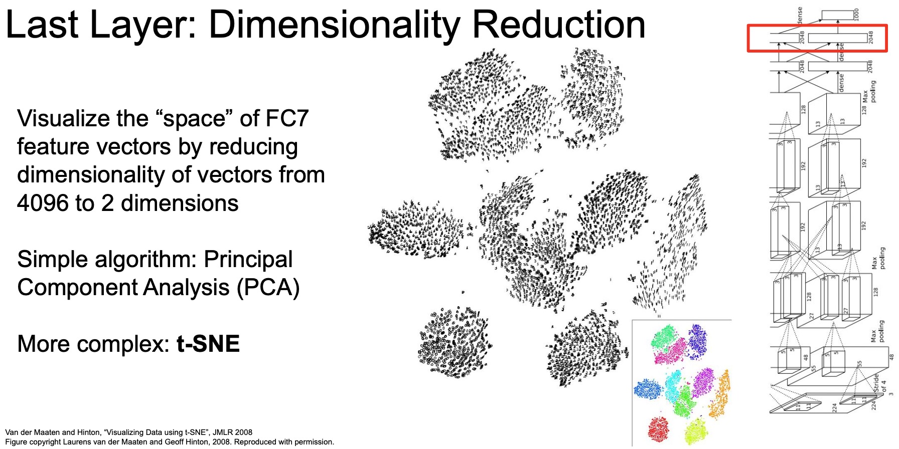
- Here we’re visualizing the ten digits in images of the MNIST dataset, which contains digits from 0 to 9 that are hand-drawn black-and-white images.
- We’re passing these images through our pre-trained convolutional neural network extracting these 4096-D vectors for each image. Once we have all of those vectors, we use t-SNE to project them all down to a 2D space.
- If we color code each of them, i.e., let each category have its own unique color, so zero is green, one is pink, etc., we notice that there’s a clear boundary and distinction between all the different digits that are learned. In other words, all the zeros are grouped together within a particular space, all the ones are grouped together within a particular space and separated from all the other classes. That’s even more evidence that what the model is learning is some sort of a semantic understanding of what it means to be a 1 versus a 3 and grouping those accordingly. If we look deeper, it wouldn’t be a big surprise to see that digits which show similar geometric patterns, say 5 and 6, lie in close proximity in this 2D space.
- Applying the same technique to ImageNet, we take some images from ImageNet and project them into this 4096-D space using our pre-trained convolutional network. We further project them back down into a 2D space and then we lay them all out in a nice grid like fashion (shown below).
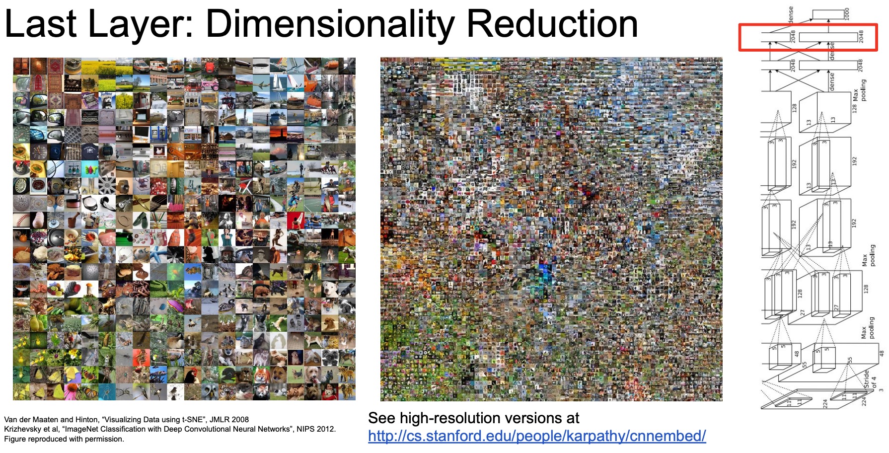
- For every single point in the grid, we find the nearest image to that point and we place that image in that particular location.
- A zoomed-in version is on the left and in the middle you’ve got a zoomed-out version with thousands of images that have all been placed within that space.
The reason you might want to build out these kinds of visualization techniques is because it gives you a sense of what the model is learning. It also gives you an understanding of the geometry of this learned embedding space.
- To elaborate on the geometry aspect a bit, if you look at this zoomed-in image on the left, you’ll notice at the bottom left there’s a bunch of butterflies of different colors, shapes and orientations, but they’re all grouped together and as you move from that bottom left to the right you see that the butterflies eventually turning into birds, turning into wolves and dogs. This should give you a sense of what are the sort of categories that the model has learned that are also similar to one another.
- Wolves and dogs are in fact relatively similar. Having those next to each other is giving you an idea of the geometry learned by the model after you’re trained it on ImageNet.
Visualizing internal representations/activations
- So far we’ve been talking about this last layer. Now, let’s move on to visualizing and interpreting internal representations.
Recall our discussion about the difficulties in understanding/visualizing the weights of these internal representations so instead of understanding the weights, let’s visualize the activations instead.
- Note the terminology here.
- Weights are the learned parameters of each of the convolutional/linear layers.
- Activations are the outputs of each of the layers, which get passed on to the next layer.
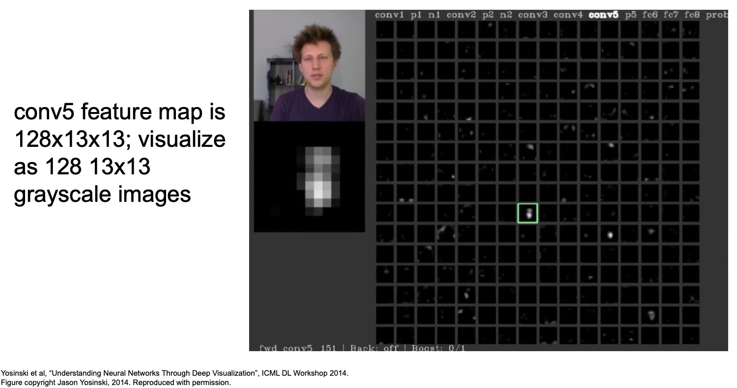
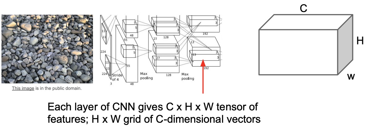
- At a workshop in ICML 2014, in “Understanding Neural Networks Through Deep Visualization”, Yosinski et al. visualized the activations of different parts of AlexNet. After passing in the particular image of the person on the top left (shown in the figure below), we observe the outputs of the CONV-5 layer, which is a \(128 \times 13 \times 13\) feature map, visualized as \(128\) such \(13 \times 13\) spatially-sized images, one for each of the \(128\) channels.
- We’re taking all of those \(128\) images and laying them out in this grid and each element on the grids represents a \(13 \times 13\) activation.
- Most of the activations are black implying that they’re not actually activating and there’s no outputs that are being generated. However, there are a few channels that are being activated and do produce some sort of output. In face, there’s one that appears like it’s focusing on the parts of the image that the person is appearing in.
- We can thus use techniques like this to figure out what are some common things at a particular channel in a given layer activates to. While it’s hard to interpret the weights just by themselves, we can pass in a ton of images through our model and look at the common things that a given channel within a specific Conv layer activates to, and use that to make an interpretation on what we think that channel is really focusing on.
- (+) This might not be evidence that this channel is only focusing on faces but it can atleast serve as a clue that perhaps it is and perhaps if we passed in more images, we can be more certain about what that particular channel in the Conv5 layer of AlexNet is really looking for.
Patch-level maximal activation analysis
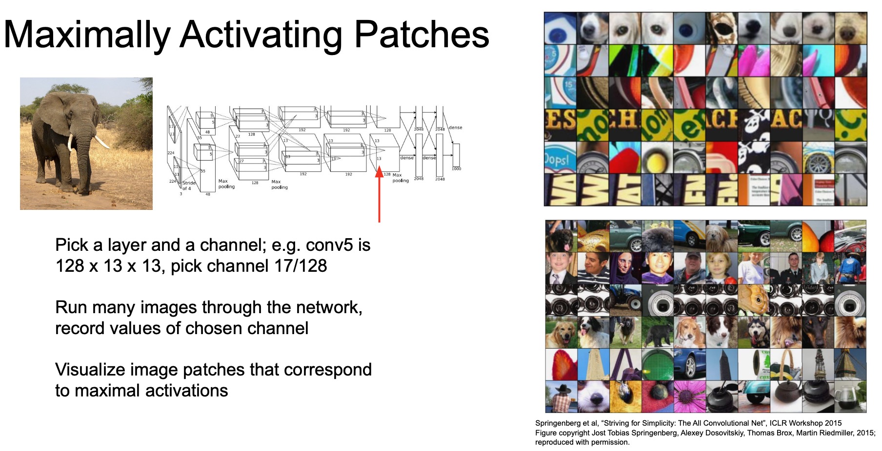
- What does it mean to maximally activate a class? Essentially, we’re looking for an image template that leads the model to classify a test image which follows that template as belonging to a particular class. Let’s assume a score can take values from 0 to 1 so to maximally activate it that score needs to be as close to 1 as possible. So we assume that the class score is 1 (since we’re looking to maximally activate a particular class and we’re working with a images from the same class) and back propagate using the class score.
- You can do this the same thing with internal representations as well, since you just want to make sure that you can maximize the activations you care about (and not class scores in this case). Let’s say you take an input image and get a value for an activation that you care about. Next, instead of minimizing that activation like you do with a loss (with gradient descent), you minimize the negative of that which meets you are maximizing the activations and then you back propagate with those maximized activations.
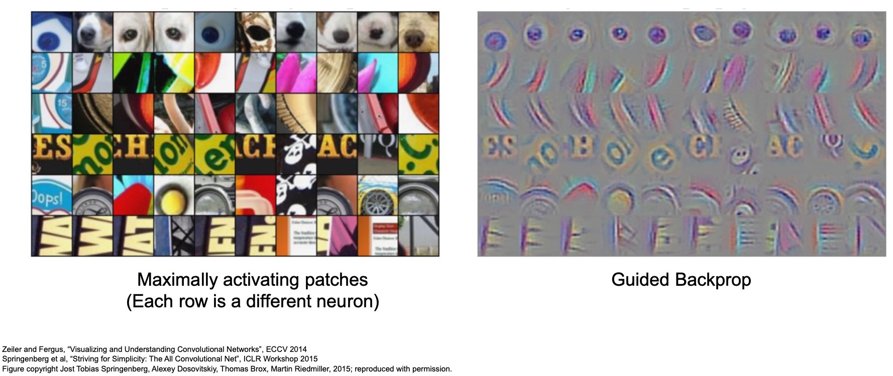
- Generalizing this idea, we can pass in tons of images and measure what are the top patches of images that get activated given for a particular layer, by visualizing each channel of the output activations one-by-one.
- Each row of images on the right represents a particular channel in a particular layer, in this case channel 17 out of \(128\) for Conv5, and what kinds of patches of images they are activating the highest to or reacting the most to.
- We’re simply building on the intuition we developed in the previous section, but now we’re applying it here at a larger scale by passing in tons of images from our test set and looking at the kinds of patches of images that get activated for a given channel.
- Notice the very first channel looks like it’s really attending to round blob-like structures that are usually darker in the middle and then lighter around it. Often picking up eyes as well and sometimes noses of dogs. Looking at some of these other rows, some of them are specifically picking out people’s faces, some of them are looking for round black circular structures. Others are activating primarily to dogs, some are activating to different kinds of flowers. Some are activating to what looks like text in our images.
- (+) This gives us an idea of all the different kinds of stimuli that the particular Conv layer seems to be looking for within our pre-trained network.
Which pixels matter: Saliency via Occlusion
- Zeiler and Fergus proposed another way of measuring exactly what our models are learning in “Visualizing and Understanding Convolutional Networks” (2014) by blanking/occluding out parts of the image and then seeing if our output prediction has changed.
- In the paper, the authors proposed a bunch of visualization techniques and a lot of them are popular even today and are used in more advanced forms.
- (+) Saliency via occlusion involves taking a blank patch and running it across the image and feeding each patch-“iteration” of that image through the model to see what parts of the image are most important when making a prediction for a particular class.
The idea behind occlusion experiments is to mask part of the image before feeding it to your ConvNet model and draw out a heat-map of the probability that the image still belongs to its class at each mask location. This will yield the most important parts of the image that the ConvNet has learned from.
- For this given image of an elephant, the authors found that if you put a patch on the bottom right (in the region of the ground) it doesn’t actually impact the score of the elephant, because the model still outputs a high elephant score of \(0.95\). But if you hide the center of the elephant, in the region of the elephant’s face, the score for the elephant goes down to \(0.75\) indicating that perhaps that part of the image is most important for the model to infer a prediction that it’s an elephant.
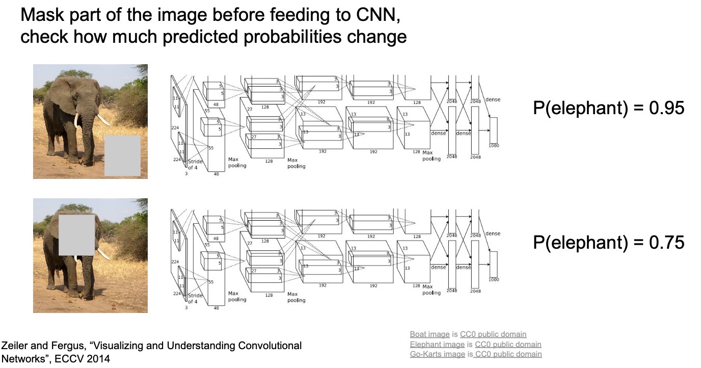
Thus, saliency via occlusion functions using a sliding window approach where you slide a patch across the entire image. Next, for every single sliding window location, measure how much the score of the correct class drops. This gives us an indication of what parts of the image are most salient for that particular category/class.
- The figure below offers a visualization of what that would look like if we ran that sliding window through the entire image. Looking deeper, you notice that the elephant’s face and its tusks (the most unique characteristics that identify an elephant) seem to be the most important parts here.
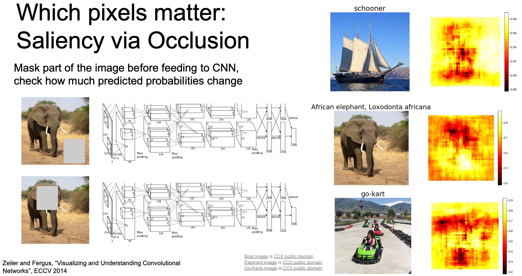
- Note that dark red implies that it leads to the lowest reduction of the score for the correct class implying that that is the part that is the most important when predicting the correct class.
- Similarly if you look at the ship, it appears like it’s the the actual ship that’s most important and the model ignores the water around it. Likewise, for the go-cart, it looks like it’s really focusing on the parts of the image that represent the go-cart when making the prediction.
Which pixels matter: Saliency via Backprop
- Saliency via occlusion makes you wonder that we can even do segmentation by combining these kinds of techniques.
- Introducing saliency via backprop. We’re given an input image, and we figure out what class it is by doing a forward-prop through our model. Next, you backprop using the gradients of the loss w.r.t. the input image, \( \frac{dL}{dX} \) (instead of the gradients of the loss w.r.t. the weights, \( \frac{dL}{dW} \), which is how vanilla backprop works) to try to figure out what are the most important parts of the image that represent that given class.
Specifically, we try to maximize the activations for the dog class by computing the gradient of the unnormalized class score with respect to the input image pixels, take the absolute value and max over all 3 RGB channels and backprop this value into the blank image. This yields a gray image that represents the most important areas in the image.
- In this method, we start with a random blank image and we backprop into that image from the activations produced by an input image and use that to figure out what are the most important parts of the image that correspond to that given class.
Unlike backprop where you calculate the gradients with respect to the weights of the network, we are now calculating with gradients with respect to some blank input image that we start off with.
- In the specific example show in the image below, we’re using a saliency map to identify the parts of the image that led to the most activations in the model.
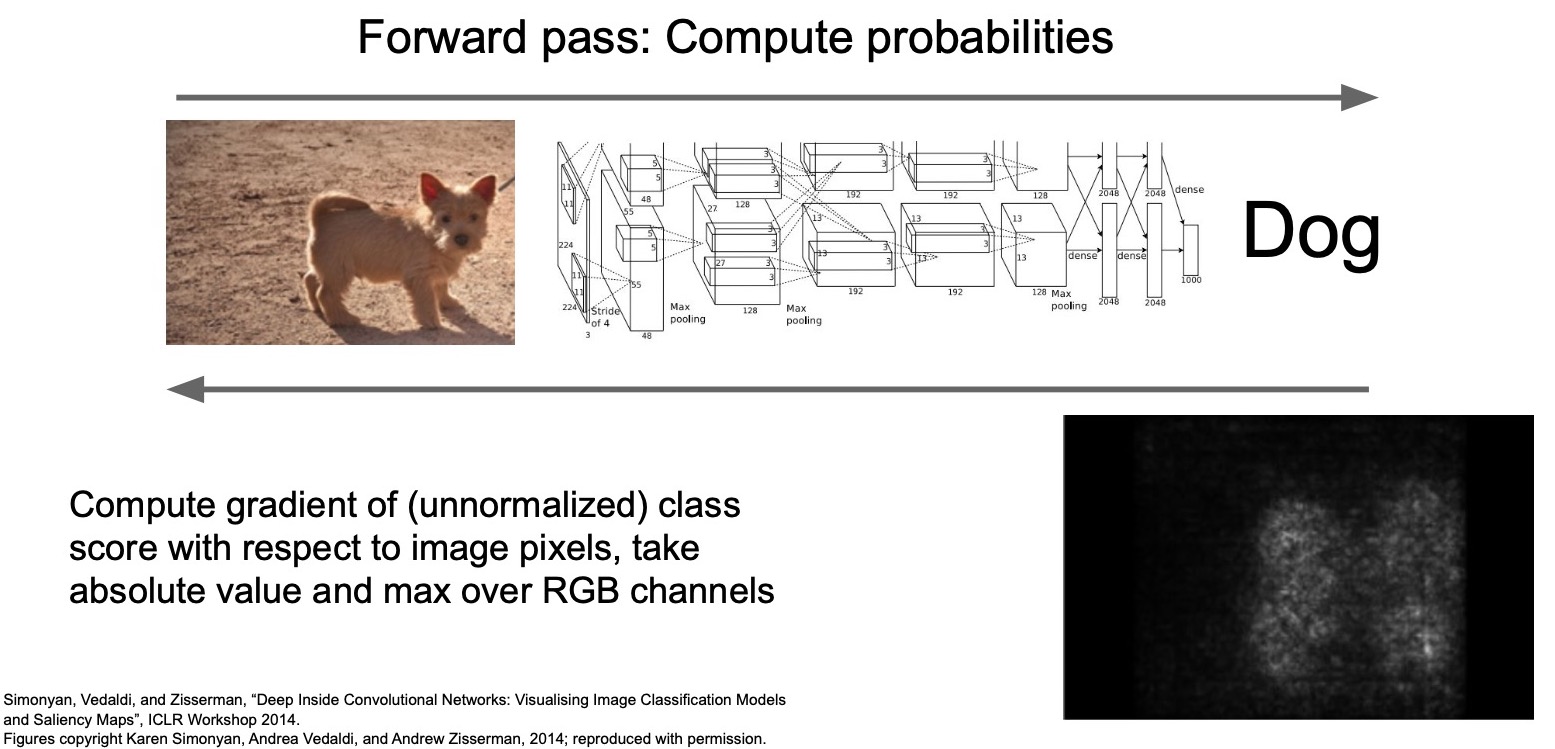
- The image above shows the part of the image that represents the features of the dog which the model should be attending to. Note that in the majority of the image, the gradients are zero indicating that even if those pixels change by a little bit, it won’t impact the score of the class. But if the pixels where the dog is located change, then it will impact the final score.
- Below are some other examples of saliency maps where images that were passed into the network, class-scores were obtained using forward-prop and then we backprop into an empty image to try to maximize the activations for that given class.
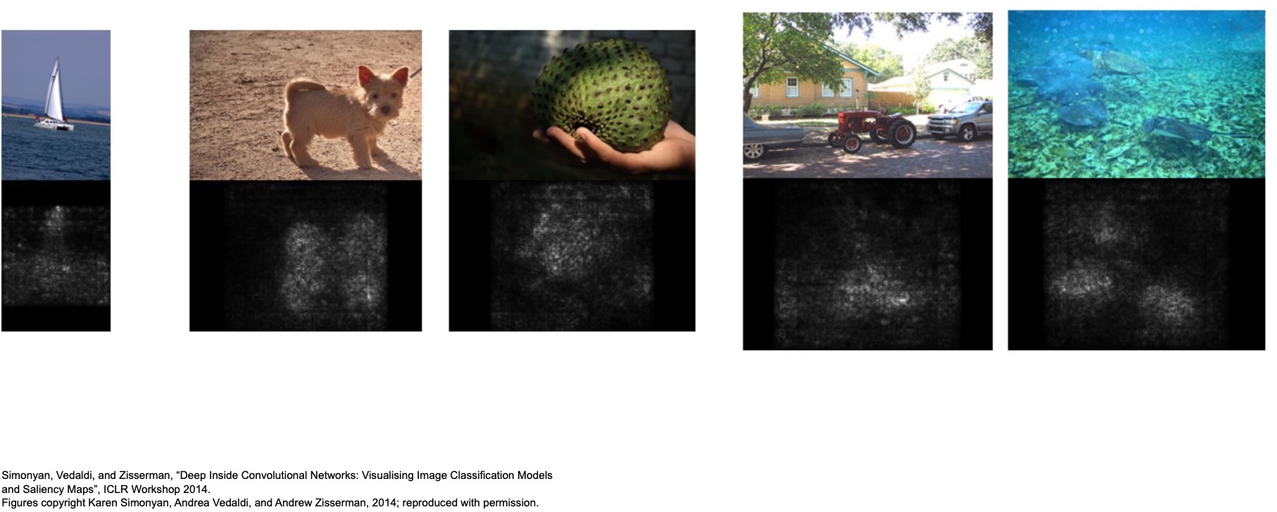
- (+) It looks like the model is learning what parts of the image are most important when making predictions for these classes because those parts of the image are being highlighted as the gradients are flowing back.
Saliency maps + GrabCut: Segmentation without supervision
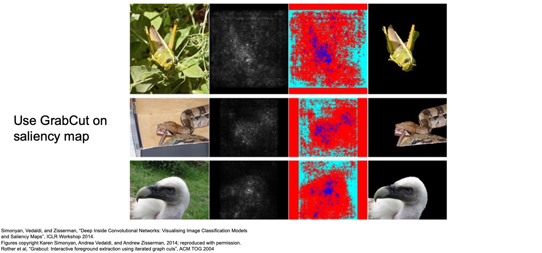
- Combining saliency maps with an idea called “GrabCut”: interactive foreground extraction using iterated graph cuts (2004) by Rother et al. where you interactively figure out exactly what part of the image contains the object that you care about, and you can use this to do segmentation.
- Recall that segmentation involves finding the exact pixels that correspond to the correct class.
- Here, we can do the same thing without any actual segmentation labels but but just by training a classification model and then back-propping the activations to maximize for the specific input regions that lead to that correct prediction.
- Combined with GrabCut which helps you refine exactly what parts of the image matter, you can come up with really nice clean segmentation masks for your models.
- Note that this kind of a method does not does not perform as well as the segmentation methods we talked earlier where they have explicit human-labelled annotations for each of the images but it still does reasonably well. You can use such a technique to interactively generate large training data for segmentation.
- Obviously, segmentation is a really costly operation because we need to figure out exactly what parts of the pixels matter. Using a technique like saliency via backprop, you can build systems that allow you to easily annotate large amounts of data by minimizing the amount of human supervision or annotation that’s needed.
Saliency maps: Uncover biases
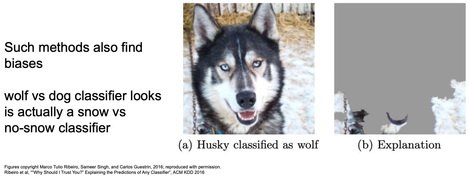
- In “Why Should I Trust You?: Explaining the Predictions of Any Classifier” (2016), Ribeiro et al. trained a dog vs. wolf classifier using saliency techniques to figure out exactly what parts of the image are the most important when we’re making the distinction between dogs and wolves.
- They found the model in fact wasn’t really learning a dog vs. wolf classifier. It was instead learning a snow or no snow classifier because wolves in the training set were primarily found in in snow. So the model figured out that it was too hard to learn to distinguish between dogs and wolves but if it just learns how to identify snow, then it’ll do a lot better on its training set.
- These methods help you understand biases that can creep into your networks by using concepts like saliency maps to figure out exactly what parts of the image that your trained model is actually looking at (i.e., the underlying visual attention).
Guided Backprop
- Another paper by “Striving for Simplicity: The All Convolutional Net” (2015) by Springenberg et al. followed up on this line of work and introduced a technique called guided backprop.
- So far we be talking about just applying backprop and measuring or visualizing the gradients with respect to the input image. They were specifically interested in a variation of backprop that creates even nicer visualizations of what parts of the image really matter.
- Just like last time we want to do the exact same thing we want to identify which portions of the input image caused the specific activations in a particular channel in a given layer.
- We can do this by back-propping those activations from that layer or we can do a specific variation of back propagation that we’ll describe here called guided backpropagation.
- The main idea behind guided back propagation is explained in these four steps in the figure below.
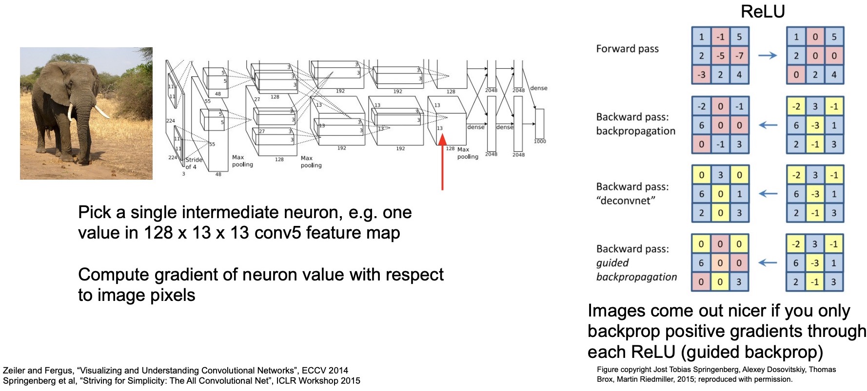
- Let’s say that you’ve got some input that comes into a ReLU layer. Given the zero-thresholding nature of ReLU, it allows passing in all the values that are positive. In blue are all the positive values, which get forward propagated. All the values that are negative in red get set to zero.
- During the process of backpropagation, we obtain gradients (using the chain rule). Gradients for positive values get passed on, but those for negative values in our input are 0.
- In guided backpropagation, all the gradients that are negative from the ReLU layers are also changed to 0. That is the only change they make to the back propagation algorithm.
-
The intuition is that they only want to backprop those gradients from the ReLU layers that are positive because they want to identify the features that lead to a specific decision. They don’t care about the absence of a specific feature. In other words, they only allow gradients from ReLUs to flow back if those gradients are positive for which the inputs were also positive, because ReLUs by itself make sure that only the input positive values propagate through while the input negative values get set to 0 as well as their gradients.
- In the figure below, we’re visualizing some examples where you see some really interesting patterns emerge because now not only can we pick out exactly what patches are most important for a given channel in a given layer, but now we can figure out what parts of those patches are the most important. Our intuitions were right when we were thinking about what each of these specific activations were really looking at – it looks like the top row the channel that we’re visualizing which we earlier thought was looking at round blob-like structures, does in fact look like that’s true because those are indeed the parts of the patches that it picks out. Similarly, the one that’s picking out letters is in fact looking for letters because those are the positive gradients that are being back propagated back using guided backprop.
Guided backprop thus relies on the fact that the generated images come out nicer if you only backprop positive gradients through each ReLU.
- The figure below shows some more examples. Again, it looks like there are specific channels that are activating to dog faces, people’s faces, car wheels, etc.
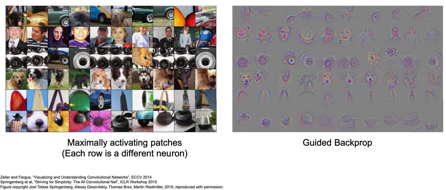
- (+) By passing in a large set of images through your network and measuring exactly what parts are causing maximal activations, you can interpret each of the channels in a given layer using this technique to build an intuition as to what parts of the image the channels are really looking at.
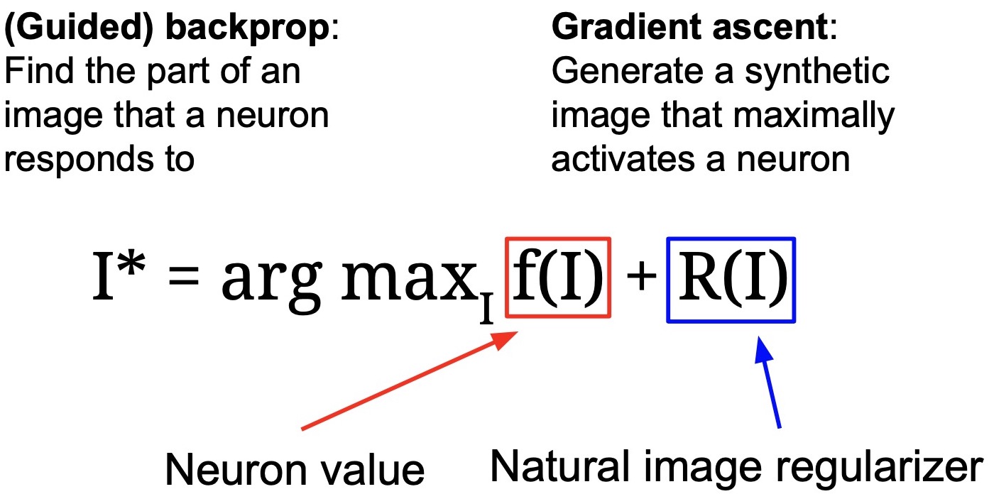
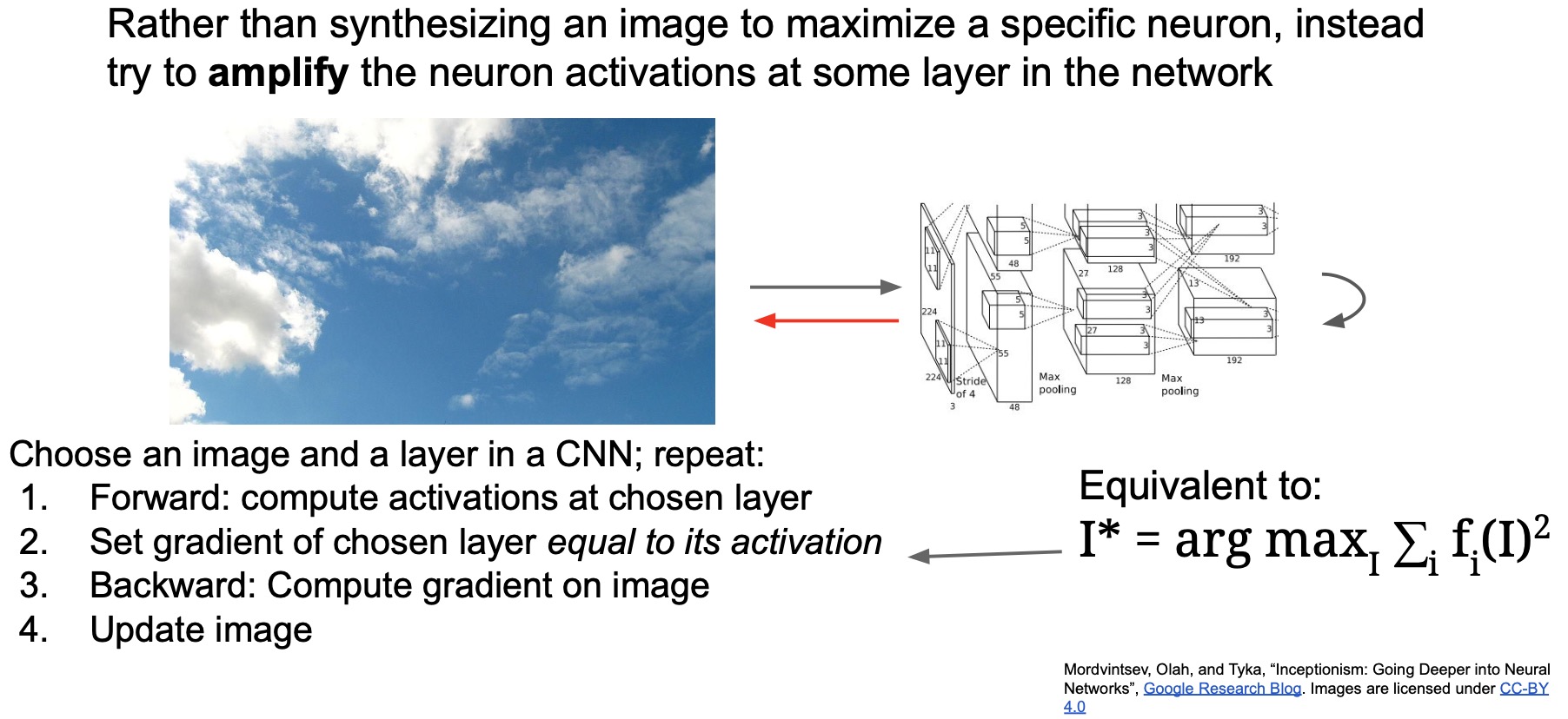
Gradient Ascent
- So far we’ll be trying to interpret these channels within layers using data sets of images and we’ve been looking at patches and map cropping into the regions of the image that are maximally activating specific channels in given layers.
- Another way to visualize CNNs is to figure out what kind of image maximizes an activation in a neuron or what kind of an image achieves the maximum score for a specific category/class. As an example, what is the most stereotypical prototypical image of a dog that the model reports the maximum score for as far as the dog class is concerned, and minimizes the score for all the other classes?
- Thus, the question arises: what if we continuously backprop in an empty image to maximize the activations of a specific new neuron or maximize even the last class score for a given pre-trained network.
- We can do that using a technique called gradient ascent. It’s essentially the same thing as back propagation, except now we start off with some random image and we continuously backprop into that image to maximize the activations at a given layer in the network.
-
With gradient ascent, we are trying to learn the image that maximizes the activations for a particular class:
\[I* = \mathop {\arg \max }\limits_I(f(I)) + R(I)\]- where,
- \(R(I)\) is a image regularizer.
- \(f(I)\) is the neuron activation (i.e., the neuron “value”).
- where,
- Formally, we’re trying to find \(I*\) which is the the maximally activated image input that causes \(f(I)\) which represents the specific activation you care about. You can also interpret it as the final class score that you care about. In general, it can be function you care about
- \(R(I)\) is a regularizer to make sure that the generated image is actually a realistic image and not something that doesn’t even resemble a real-world image.
- There are different kinds of regularization that you can use to produce naturalistic images but for the large part, even if you use very simple regularizers, you get some very interesting results.
The basic idea is that instead of continuously back-propping to our weights when we trained the model, once we’ve trained the model we can backprop into an empty or randomly initialized image to try to figure out what is the input image that maximizes a specific activation.
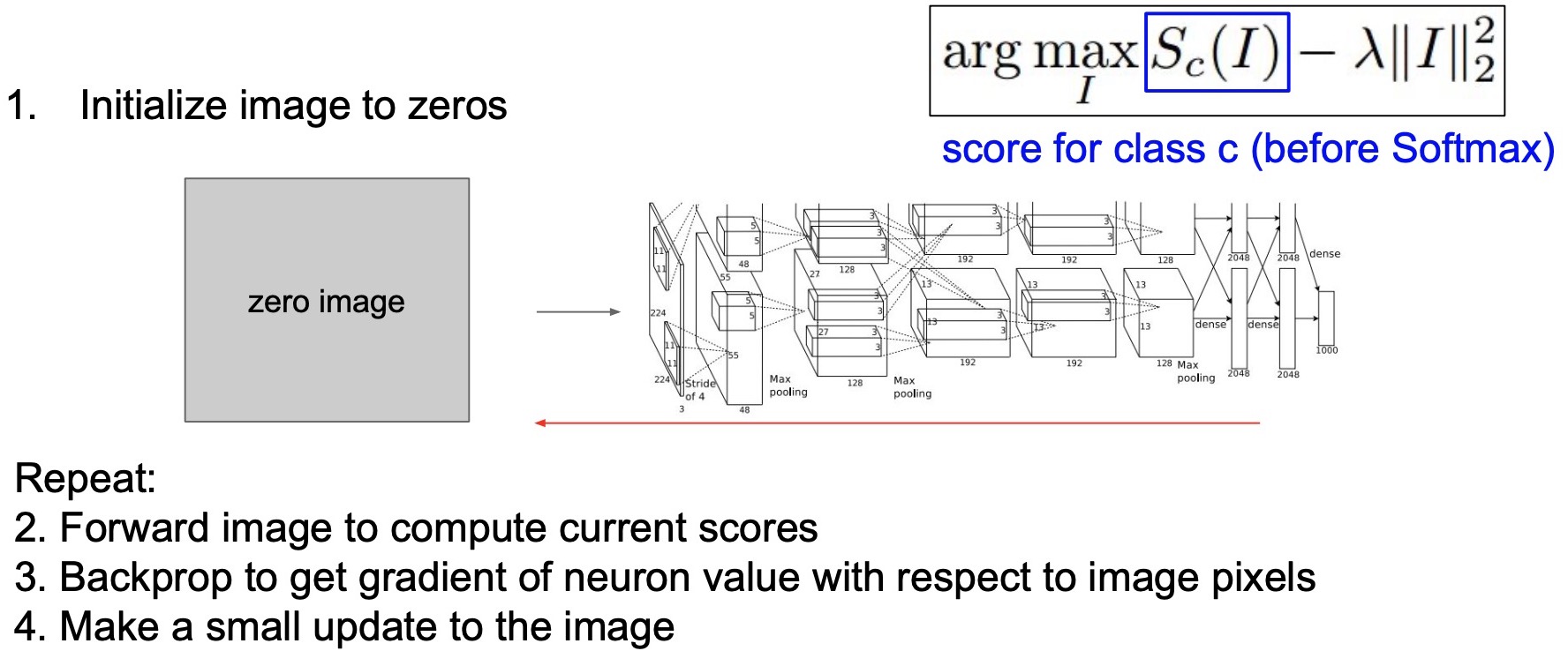
- Let’s say that you want to maximize the score for some class \(C\) then \(f(\cdot)\) takes the value of \(S_c(\cdot)\) and you’re maximizing score for the dog class.
- You start off with a zero image or a random image and continuously backprop until you generate an image that maximizes the score for dog.
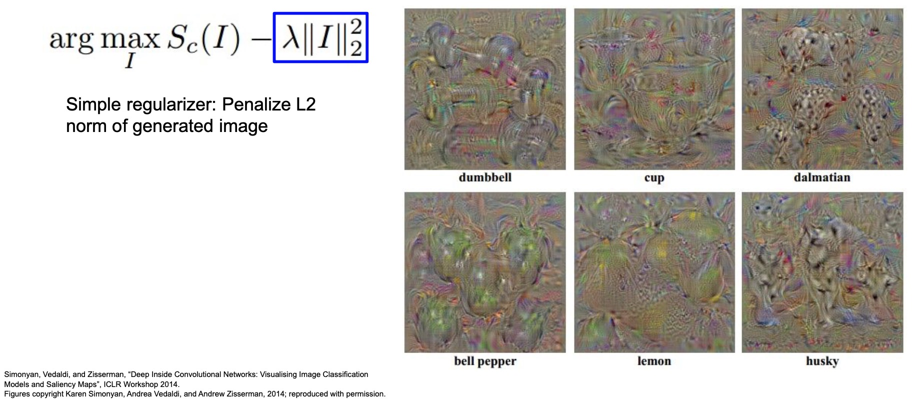
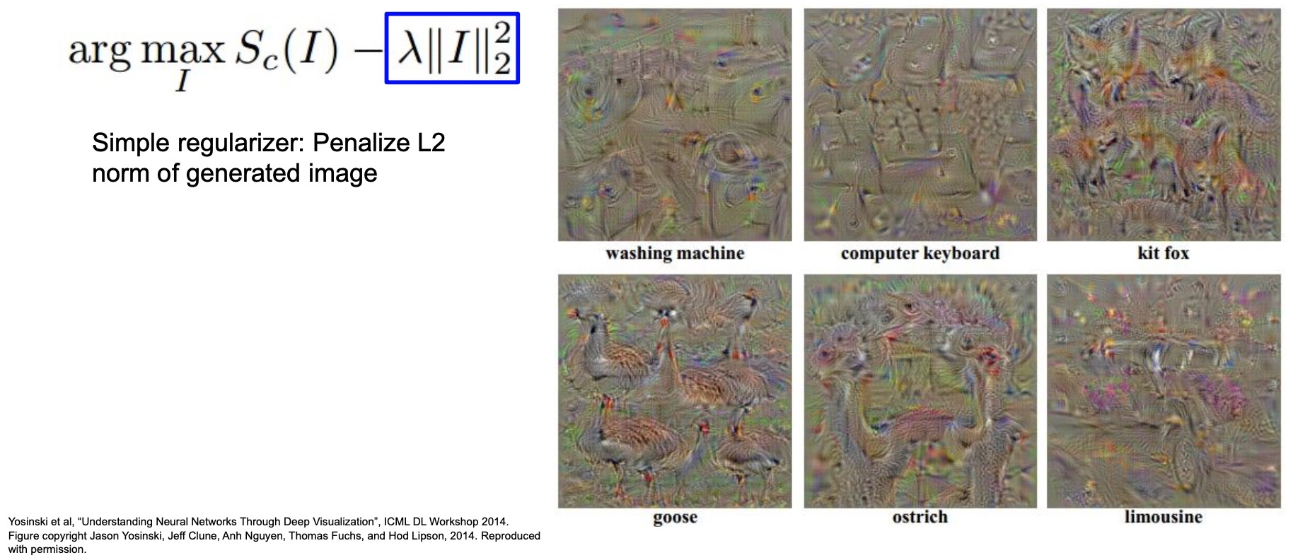
- You can use a simplistic regularization technique such as L2-norm. With regularization, what we’re essentially doing is essentially trying to make sure that no specific part of the image activates a lot. In other words, we want an image that has activations spread out all across the image as much as possible and no single large value.
- Even though regularization might not make intuitive sense for generating images (since we’ve used regularization primarily to avoid overfitting the training dataset by making our model as simple as possible), it does give you some very interesting results.
- In summary, here are the steps of gradient ascent:
- Initialize image to zeros.
- Forward image to compute current scores.
- Backprop to get gradient of the neuron activation with respect to the input image pixels.
- Make a small update to the image.
- The below image shows some visualizations of the generated images that maximize the dumbbells class, cup class or the dalmatians class. For e.g., in the dumbbell case, you can actually identify a bunch of dumbbells that all look like they’re on top of one another; next, you can see cups in the cup case; in the Dalmatian case, you’ll notice that it doesn’t actually generate a dog but it just puts a lot of black and white patches or parts of dogs all across the image. The bell peppers kind of actually look like bell peppers!
- Shown below are some other examples. The goose here looks really good, and so does the ostrich because they you can almost visualize the entire animal in these specific cases. Even the limousine looks pretty reasonable since it has a wheel and has really long windows which is actually a unique characteristic of a limousine.
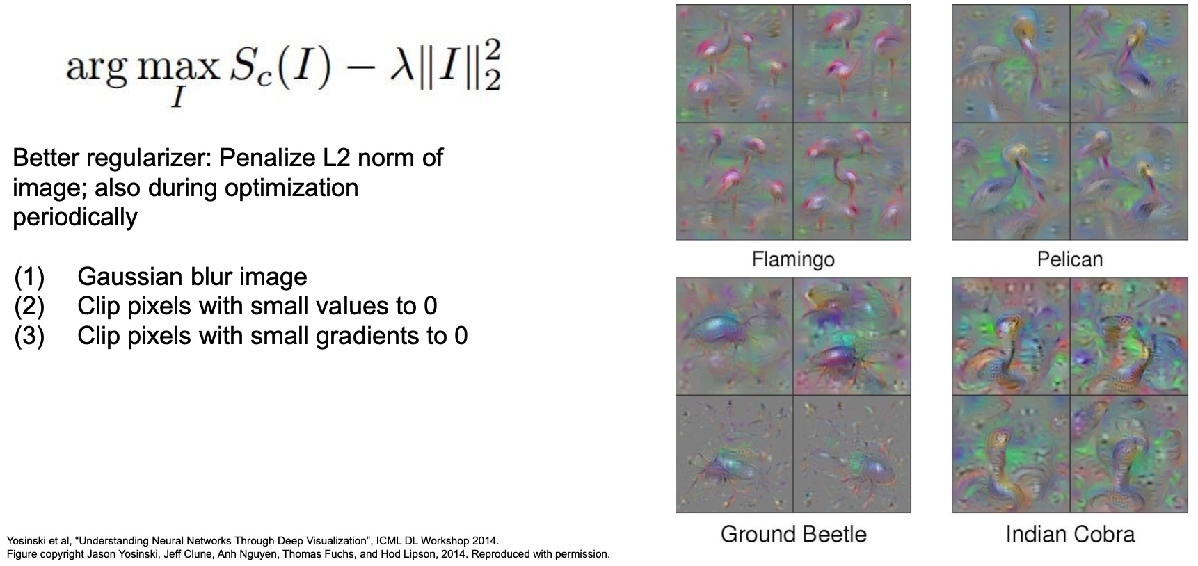
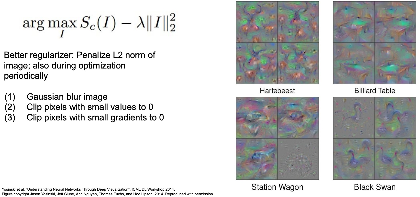
Gaussian blur: Better regularizer
- Some follow-up works tried to take these ideas and come up with better regularizer. One trick that they introduced was using a gaussian blur on the input image before passing it into the network. The reason you might use a Gaussian blur is to spread out the gradients that are coming back, so gaussian blur is basically just summing up regions of local regions of your input pixels, and so the gradients also get spread out to the local regions.
- While we still penalize the L2 norm of image in this technique just like the earlier vanilla gradient ascent technique, we also play other tricks periodically during optimization, namely the following:
- Clip pixels with small values to 0
- Clip pixels with small gradients to 0 (to make sure that pixels with small gradients don’t affect pixels that are changing)
- Apply Gaussian blur on the image
- Using these three tricks in their training, the images actually start to look even even better. You can start actually seeing flamingos, pelicans and beetles (above) and you can almost see them take the entire form you expect to see when you think of these animals.
- The figure below shows some other ones as well – notice that for the Hartebeest, you can even make out the horns. This led to a lot of excitement in the area of computer vision not just for the interpretation aspect of our neural networks but also because these are some interesting results in terms of how you can go about generating images in the first place. Note that these ideas were all pre-GAN. You can possibly do this activation visualization not from not just using the class scores but also from intermediate layers as well.
- Shown below are some visualizations of what input images look like that maximally activate different channels at Conv5, Conv4, Conv3 etc. If you look closely, you’ll see that one of the channels from Conv5 looks like it’s activating to a chihuahua, Conv3 looks like it’s looking for clothing and sometimes teeth and Conv2 (in general, the lower layers) look like they’re really activating the colors, blobs and edges – consistent with what we expect to see.
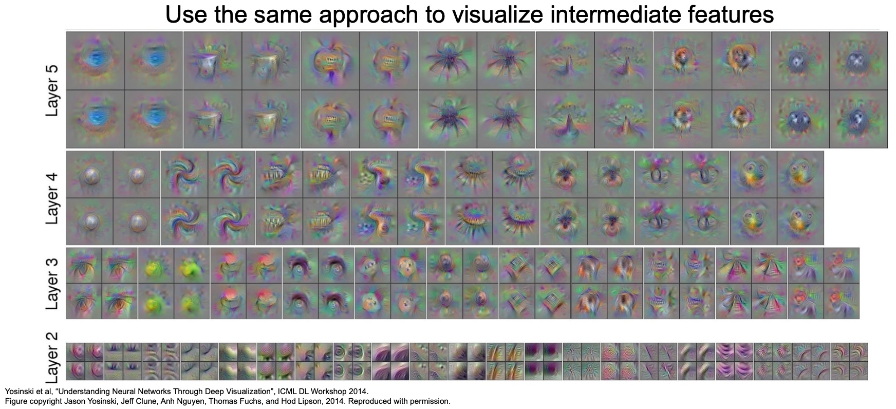
- Even though it was hard for us to interpret the weights, now we can some generate images that activate our neurons looking at a particular channel within a particular layer, and help us understand what each of the layers are really learning.
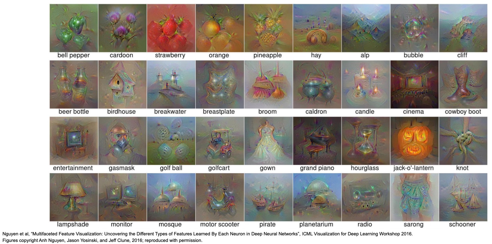
Multifaceted Visualization
- The figure below illustrates image visualizations using some additional gradient ascent-based follow-up work where you can take a specific class and there many different ways of activating to that class because a lot of our categories are multifaceted. What multifaceted here implies is that, given a grocery store for e.g., as a category, there are many different types of images that could be categorized as a grocery store, viz., an exterior of a grocery store, people shopping inside a grocery store, pictures of vegetables – so there many different “facets” to a given class.
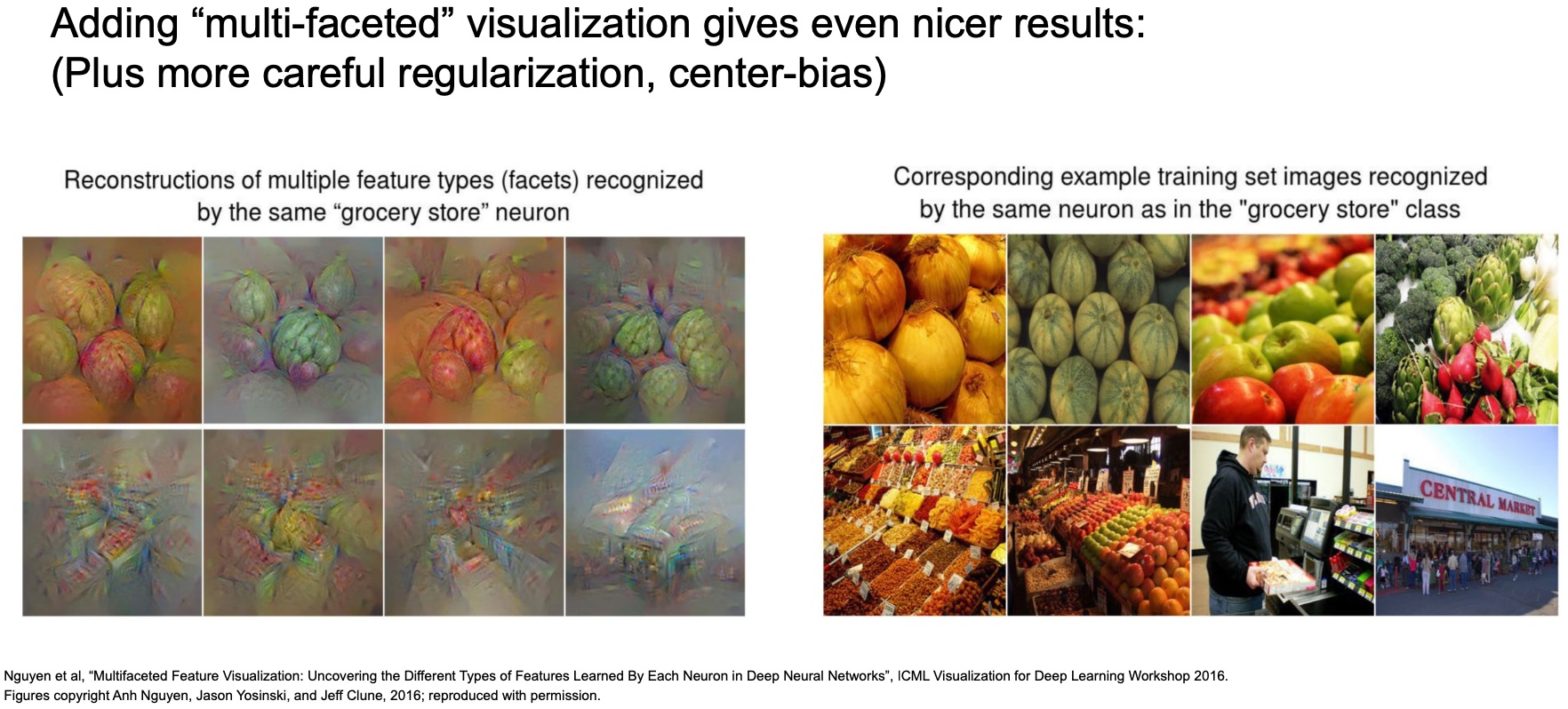
- A follow-up paper in 2016 took these ideas and what they did was they calculated the last-layer representations, i.e., the 4096-D vectors, for all of the images for a given class, say the grocery store class in this case, and then they did k-means clustering where they clustered all of the vector representations of all the images for that class into \(k\) groups, where each group you can think of as representing one of the facets mentioned above.
Next, they did gradient ascent from a sampled images from a particular cluster rather than starting off with a random image and they try to maximize the scores for all of the images within that cluster.
-
(+) The point here is that you can start generating really complex scenes – in this case, taking the example of a grocery store scene, so you’ve got pictures of fruits in baskets, you’ve got the exterior of grocery store buildings, generated using this technique. This multifaceted approach helps you generate really interesting looking images.
-
Shown below are more generated visualization examples (“steroids-induced versions of real images”).
Deep Generator Network (almost a GAN but not quite!)
- In “Synthesizing the preferred inputs for neurons in neural networks via deep generator networks” (2016), Nguyen et al. build a generator that generates images and maximizes a specific class, so it’s almost like a GAN where you start off with some latent representation which is just some vector (similar to a random vector we use as the starting point with a GAN). You want to generate an image (shown in the middle in the figure below), such that when you pass that image through a pre-trained deep neural network, it maximizes the score for the class or an intermediate activation, whatever you care about.
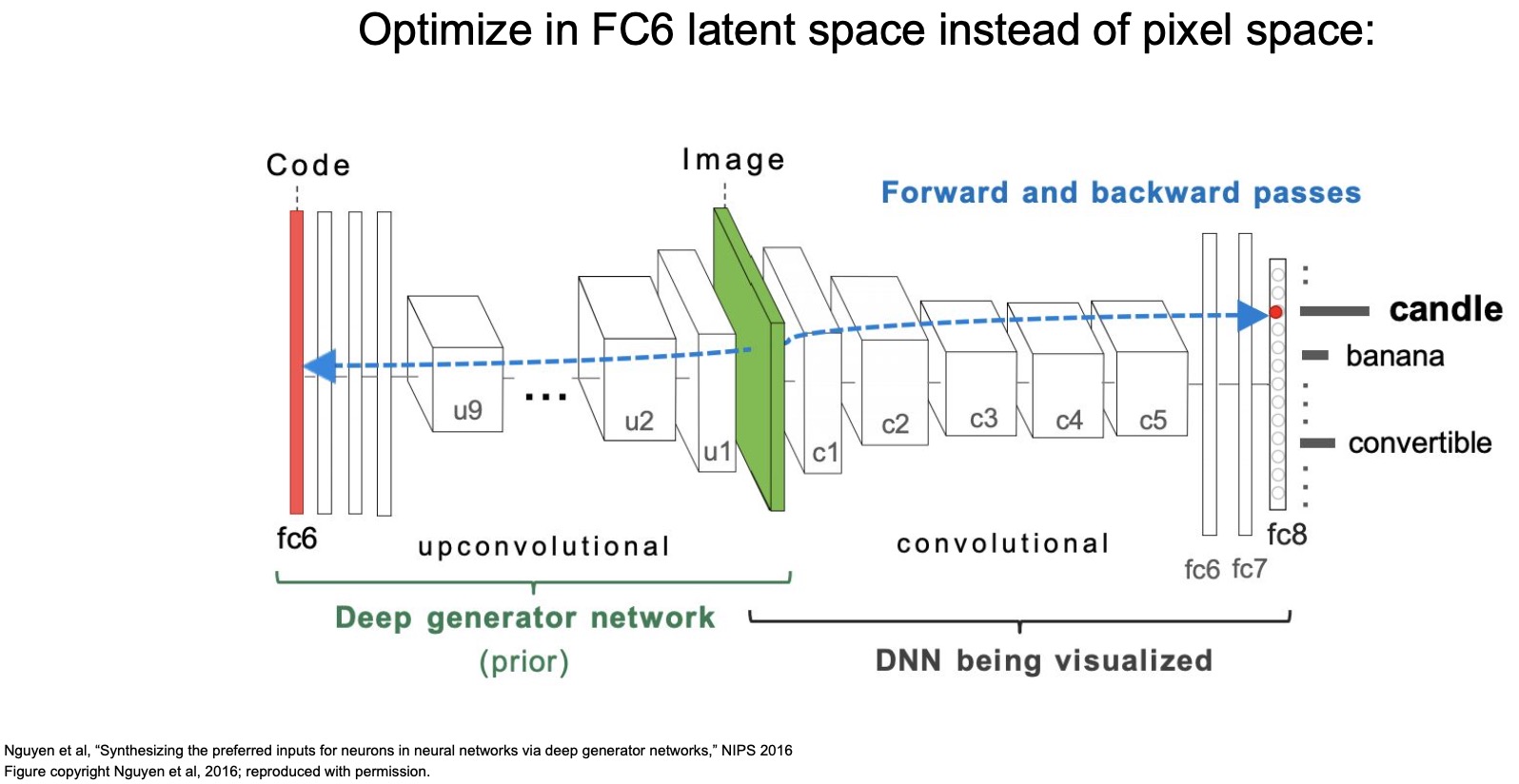
- Let’s say you want to maximize the score for the candle class, so what you do is you would start off with a random vector and you generate a random image pass it through your network, and then backpropagate to try to maximize the score of candle.
- In this case, you’re back propagating not just to the image now but you’re back propagating to all the weights of this generator network that is producing that image.
- Essentially, what we’ve done is we’ve added a generator in front of our pre-trained convolutional neural network and we’re trying to get it to generate an image and maximizes a score for a specific class.
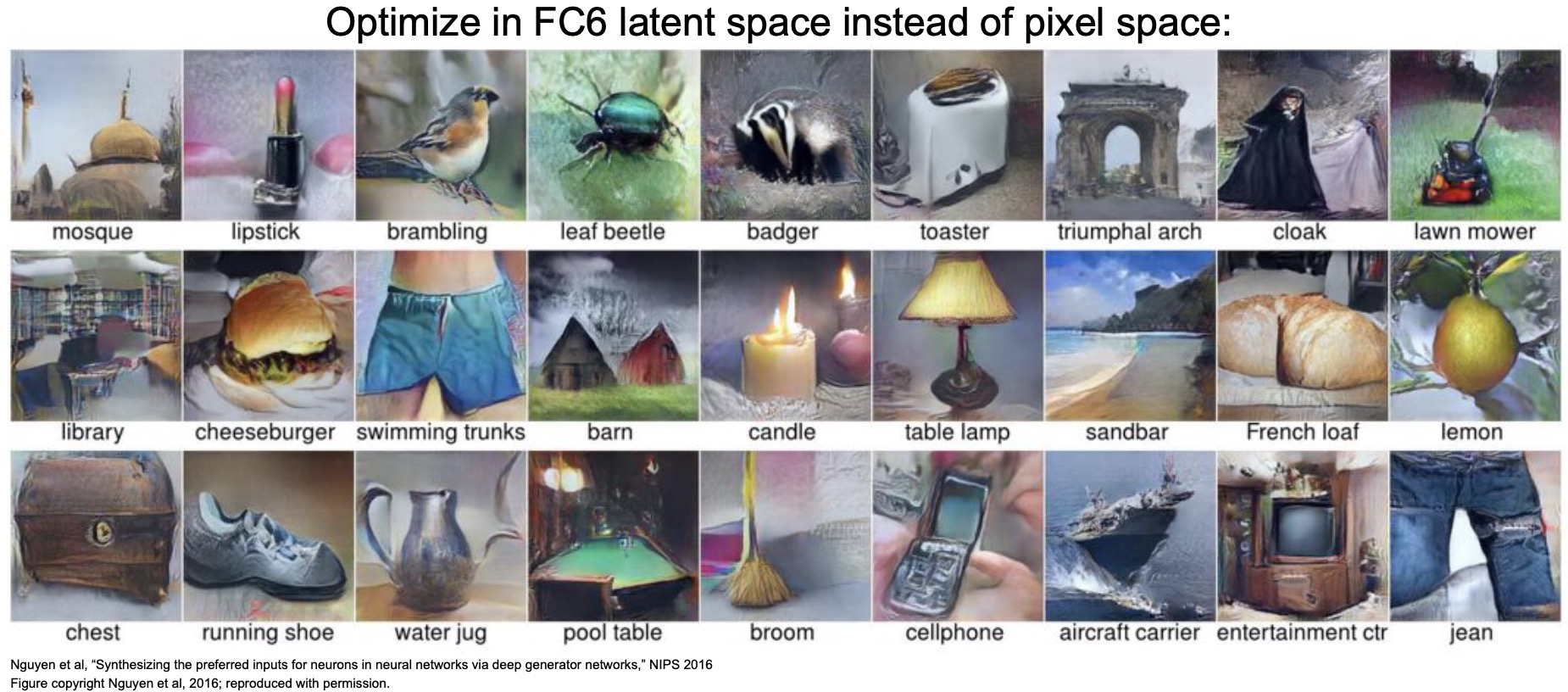
- Shown below are some examples of the outputs that it can generate. Here, we’re trying to maximize the FC6 latent space inside of the pixel space, and it looks pretty good. We are able to generate images that look like mosques, lipsticks, cellphones, grooms and table lamps.
- (+) These images look a lot more realistic than the drug-induced ones that we were looking at earlier produced using the multifaceted visualization technique. The reason is because now we’re not just trying to maximize the gradients within the image to maximize the score but we’re learning an entire network that’s trying to generate an image that maximizes a specific score, so it’s a lot more powerful because it has a ton of weights to try to generate a specific kind of image.
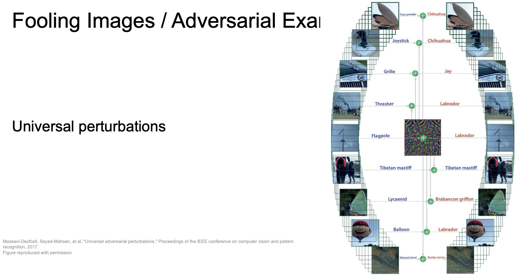
Fooling Images / Adversarial Examples
-
Since we’ve been talking a lot about modifying images, let’s talk a bit about what happens if you take an image of an elephant and try to modify it such that your network thinks it’s a koala! Essentially what we’re trying to do is we’re starting off with an existing image of a particular class and we’re going to try to make changes to that image so that it becomes another class.
-
The way we might accomplish this is, we’ll start off with some arbitrary image of an elephant and then we’ll pick another class like koala and then we’ll try to maximize and modify the gradients with respect to the input image of an elephant so that we change the image until it becomes a koala. You can interpret this as like fooling your network by changing your image into becoming something different.
- We can fool our ConvNet using the following procedure:
- Start from an arbitrary image.
- Pick an arbitrary class.
- Modify the image to maximize the class.
- Repeat until network is fooled.
- “Intriguing properties of neural networks” by Szegedy (of InceptionNet fame) and other co-authors from Google, was one of the first pioneering works in the domain of adversarial example generation.
- We’re performing gradient ascent on an input image (that belongs to class A) and trying to fool the model (such that it thinks that the image belongs to class B). In our particular example below, we’re looking to “convert” the African elephant into a koala.
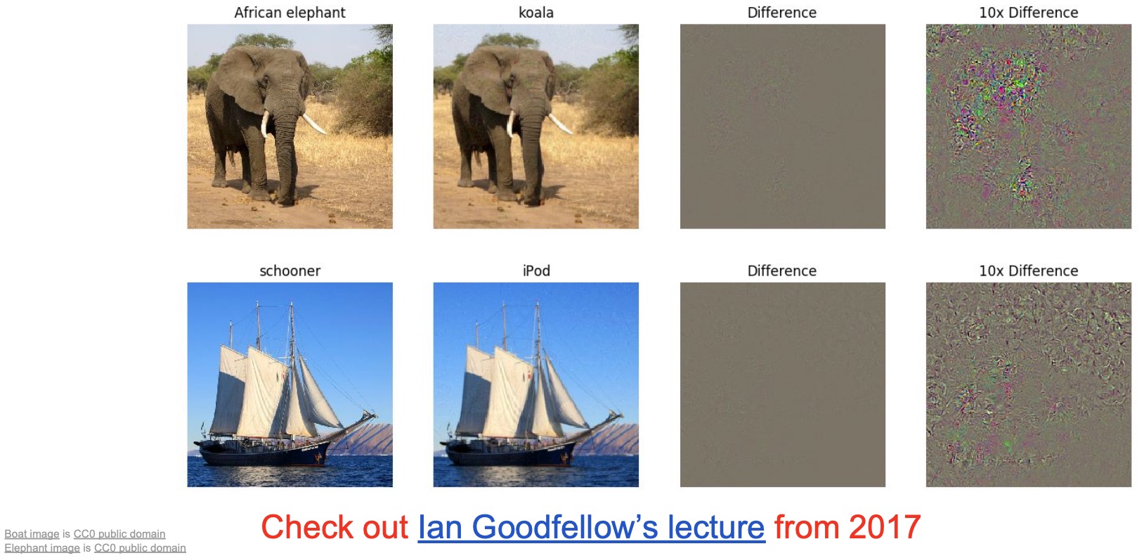
- The “difference” that we have to add to the African elephant image is denoted by the third column. That difference is enough to cause your network to think that the second image is a koala. Now, if we blow up this difference by \(10x\) to magnify exactly what we’ve changed, it actually looks like noise. In other words, we’re changing the image in a way that’s imperceptible to us.
- In fact, we can do this for any kind of images just by adding the a little bit of noise. In the second row, a schooner similarly transforms to an iPod. These imperceptible changes make the popular ConvNet models that we’ve looked at fail. In fact, they fail to classify not just one image but they fail to classify 90% of the images in the test set.
- Adversarial examples and training has led to an entire line of work in computer vision. This domain delves into thinking about how these adversarial examples arise and more importantly, what are the properties that we must have in our networks to safeguard our models from failing when when we add such noise to our inputs.
- Specifically, the line of work under the domain of “adversarial training” looks into:
- What these noise vectors are that cause all of our models to fail?
- What is the best kind of noise that we should be adding?
- Fortifying our models by training the images with added noise (but still training with the correct classes) and then train with all of those
- When is our model robust enough? (because you can prime your model as much as you want, but you don’t want to add so much that people start noticing the differences in images!)
- Specifically, the line of work under the domain of “adversarial training” looks into:
- In “Universal adversarial perturbations” (2017), Moosavi-Dezfooli et al. showed that you can learn just one single noise vector that if you add to any single image for any category/class, every single model will fail over 90% of the time. All by just adding this one noise vector that we can’t even perceive when we look at. In other words, humans would be completely unaware that the images have even been modified.
- A graphical intuition behind this idea is that when you’re training your model, you’re exploring these high-dimensional spaces of representations/activations to learn the manifold of where (real) images belonging to a particular class lie. Your model is thus learning to represent and classify images that lie within the manifold designated for a particular class. Each class has its manifold. When you’re learning this perturbation, you’re looking to figure out the boundaries of this manifold, which when crossed, lead your model to venture into “unchartered” territory where it is completely blind since it is completely off of manifold that it had learned during training. It thus behaves completely unpredictably in those spaces. Adding adversarial noise to your images thus pushes off your target image from that manifold that your model has learnt, leading to it being completely unable to classify these modified images correctly.
- There’s a line of work to quantify the confidence of a model’s prediction so that we can make easily identify such conditions where the models making predictions by “shooting in the dark”:
- “Certifiable adversarial learning or robustness” tackles this problem by giving you certificates for passing particular kinds of adversarial tests.
- People have been developing many different kinds of adversarial attacks for models that follow some sort of guidelines as to what kind of attacks are possible and so people have been building out robustness models that are robust to these different kinds of attacks.
DeepDream: Amplify existing features
- Google came up with this technique called DeepDream. It has no real practical purpose but it’s a fun way to generate dreamy-images. The ideas from DeepDream have influenced other important projects like Style Transfer.
- The approach DeepDream uses is similar to the gradient ascent method we discussed earlier:
- Forward propagate a baseline image through your model. Compute the activations at a chosen layer.
- To maximize the neuron activations in the layer you care about, set the gradient of chosen layer equal to its activation.
- Equivalent to \(I* = \mathop {\arg \max }\limits_I \sum\limits{i}{f_i(I)^2}\)
- During the backward pass, compute the gradient on the loss w.r.t. the input image, as in the case of gradient ascent.
- Execute your update rule to update your input image.
- The difference between our gradient ascent approach earlier vs. now is that we’re starting from an existing image that we already care about rather than starting from a zero/random image. We backprop the calculated gradients into our original image and thus yield some really interesting looking outputs.
- Essentially, we’re looking to “amplify” an image’s characteristics by maximizing a particular activation that we care about. Specifically in this formulation, they maximize the L2-norm of an activation of a specific layer.
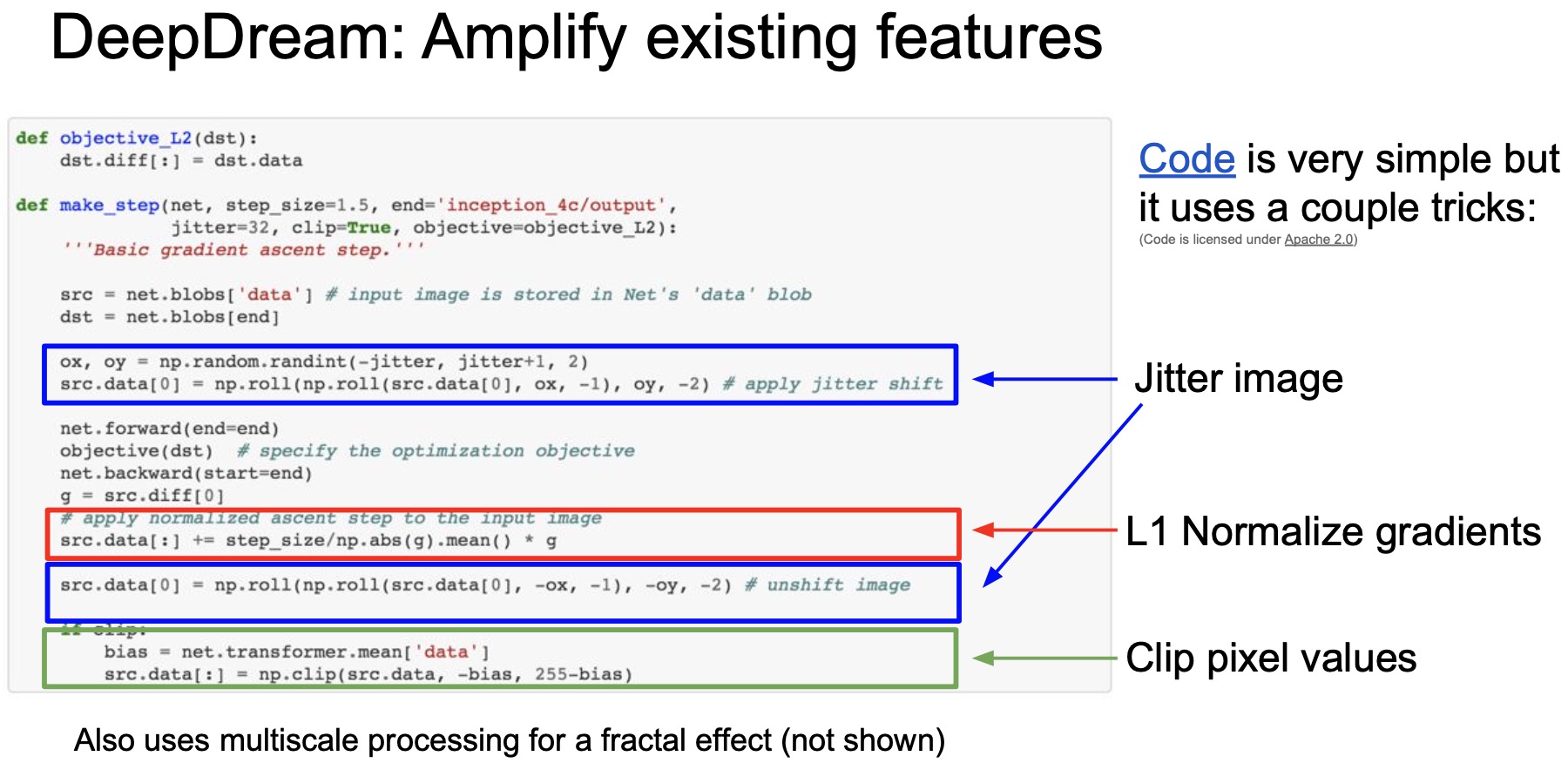
- The code for this is actually very simple. There’s a few tricks that they have to do to make this work.
- At the very top, there’s the L2-norm function, \(objective\)_\(\,L2(\cdot)\).
- Diving into \(make\)_\(\,step(\cdot)\):
- As the first step, you take the input image \(src\), you jitter it and pass it through the network using \(net.forward(\cdot)\).
- You calculate your objective which is your L2-norm using \(objective(\cdot)\).
- Perform backprop trying to maximize the objective by calculating the gradients.
- Note that the objective is the L2-norm but the figure below has an error, where it’s just using the output image \(dst\) as the objective.
- We’re basically trying to maximize the L2-norm of the activations that we care about, say Conv5 activations.
- Our loss function is a negative of the L2-norm of the activations, such that when you minimize the negative, you’re maximizing the norm.
- Perform a “gradient ascent” update step (characterized by the \(+=\)) in the new direction proposed by your backward step above.
- Because you had jittered your image earlier, you have to unjitter your image when you’re calculating the update.
- Intricate details:
- L1-normalize the gradients that are coming in. This is done to make sure that no one single gradient in a specific spatial location dominates, i.e., the gradients are spread out across all the different spatial locations in the image. In other words, you don’t get any weird sort of behavior where one specific part of the image is modified and the rest is left unchanged.
- They clip the pixel values (similar to what we talked about earlier) to ensure that anything that’s \(\approx\) 0 gets clipped to 0 and anything \(>\) \(225\) gets set to \(225\). This is done for the outputs to be within bounds for a realistic image which should be between the RGB \(\in\) \([0, 255]\).
DeepDream in practice
- Let’s start off with this image of a sky:
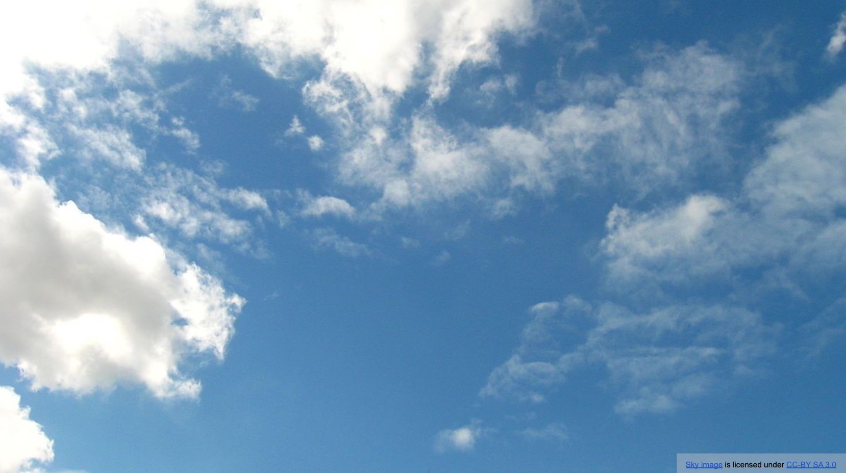
- You start updating your image and then suddenly you have these spirals that start popping up:

- You keep doing this over and over again and some weird shapes start popping up all over the place:
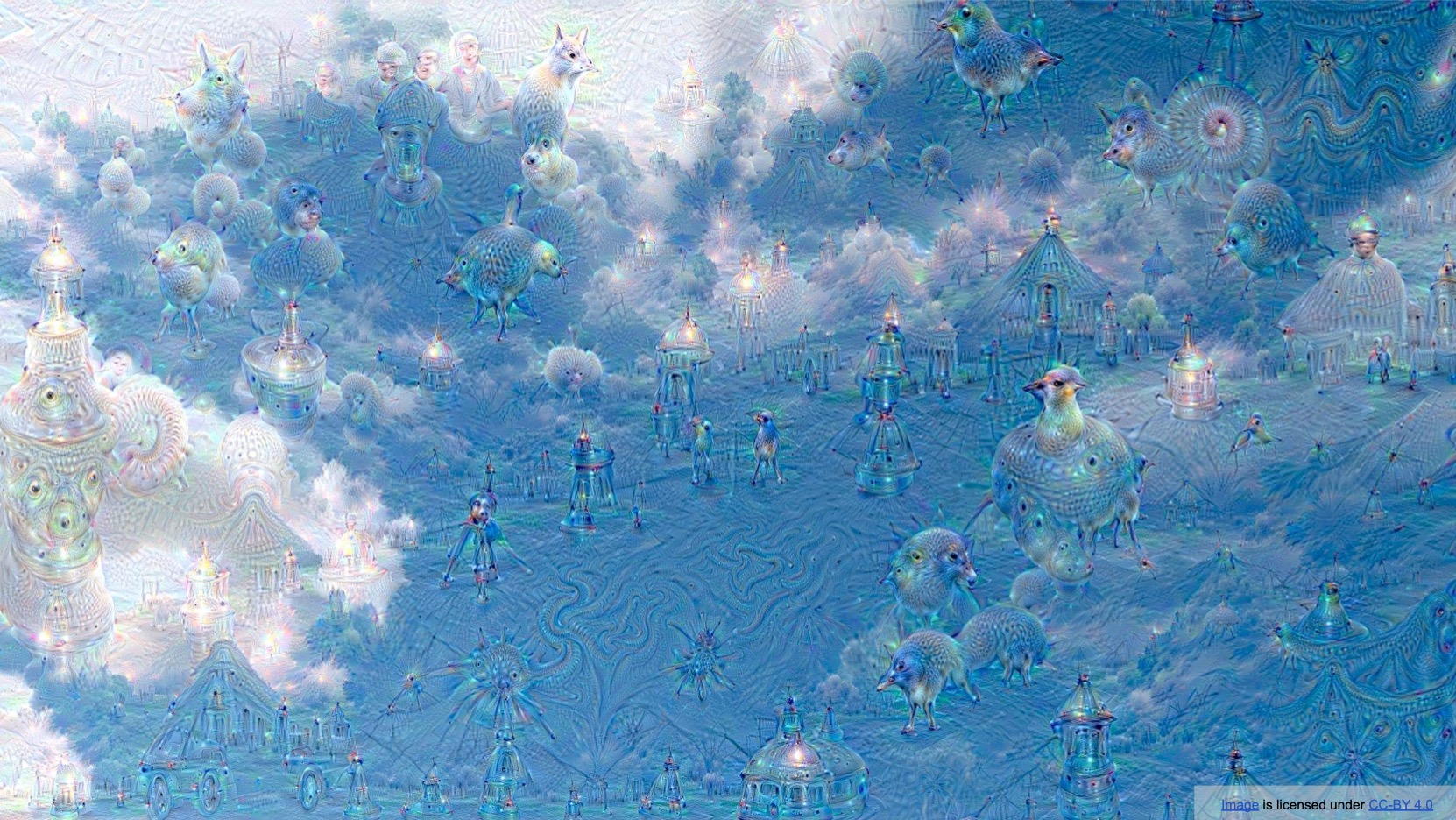
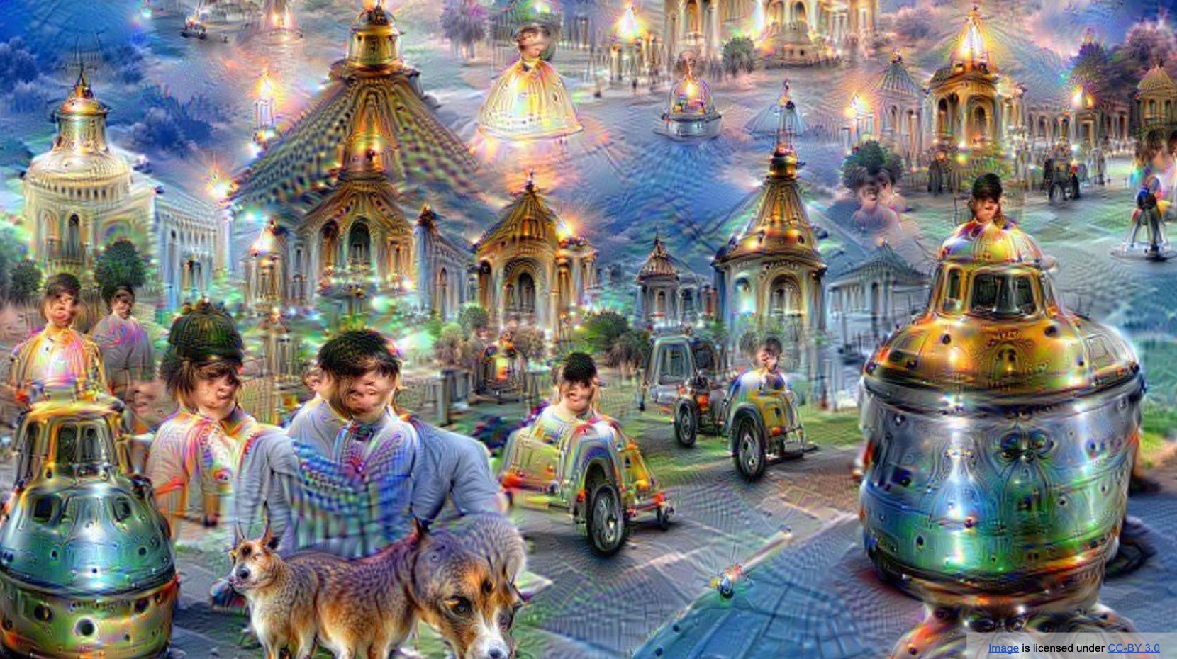
- In fact, if you train DeepDream on a pre-trained model on ImageNet, some very specific things keep appearing over and over again:
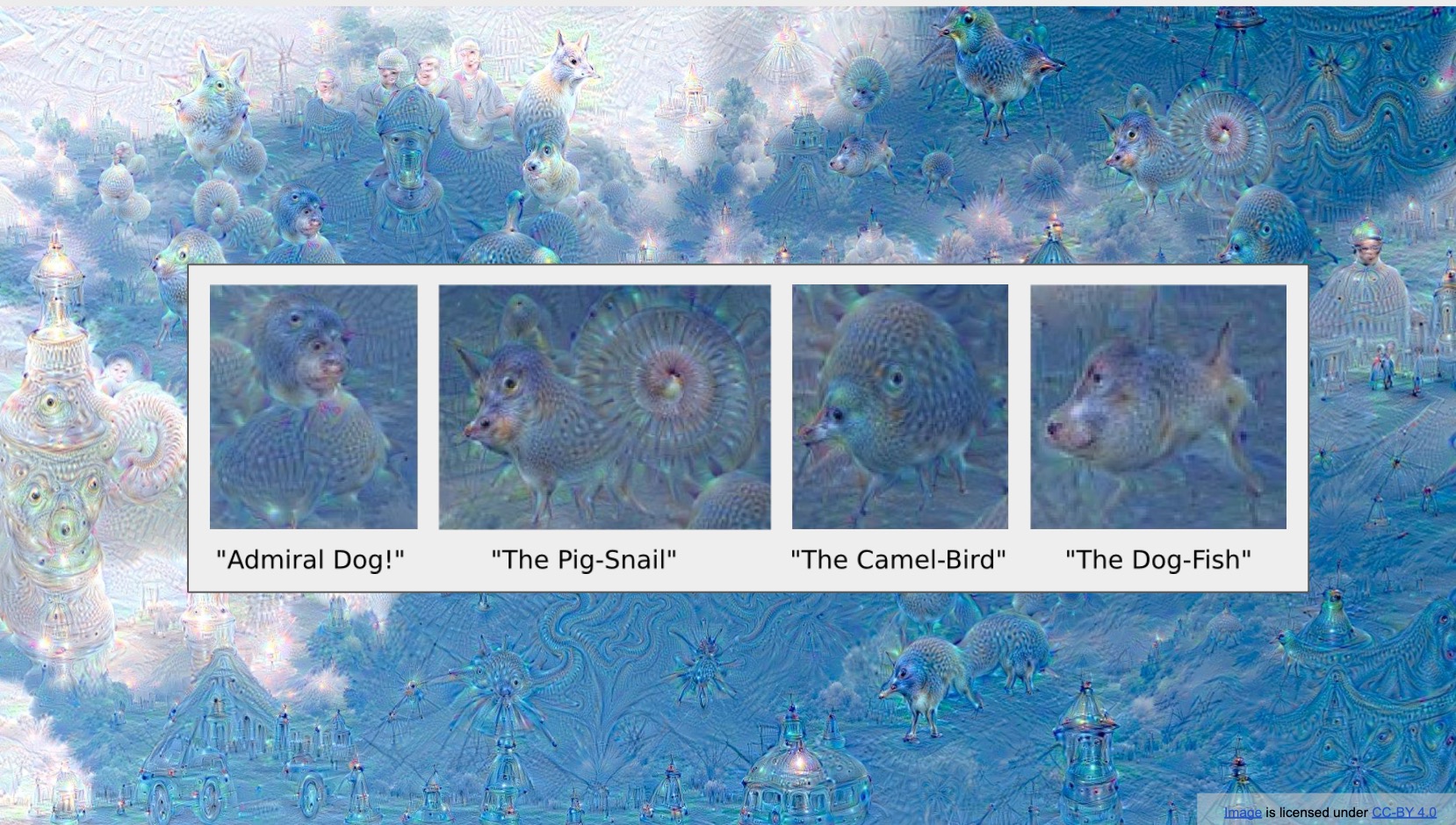
- The AI research community has been a little excited and even named some of these things that pop up all over the place so admiral dogs, or the pig snail or the camel bird or dogfish – these are common things that appear over and over again no matter what image you start off with.
- In fact, if you continue to do this at different scales and resolutions and stitch these images together, you can start getting some really interesting outputs:
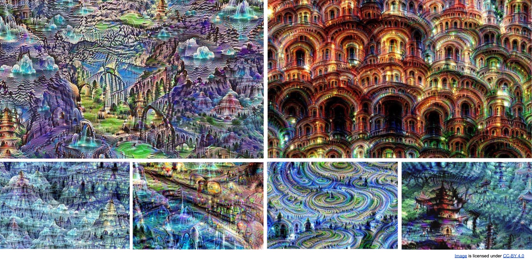
- In fact, Google organized an art exhibit where they sold off a lot of these AI generated art to a lot of people for a thousands if not hundreds of thousands of dollars each. Shown below are some examples of what DeepDream generates if you trained not from ImageNet but from the Places dataset. Unlike ImageNet, that is focused primarily on objects, the Places dataset is focused on places. Thus, what you typically find are no admiral dogs but you do find a lot of bridges, structures, mountains (and some Japanese buildings!) – those are things that pop up all over the place.
What is a CNN learning: Earlier layers vs. later layers
- In a typical CNN, as you go deeper, you’re losing spatial information because of down-sampling at each layer using say, MaxPooling or global average pooling, leading to a spatially smaller output volume. However, at the same, you’re also increasing the channel width as you go deeper by using more filters (which leads to the accumulation of several types of features, say different types of edges being put together to identify a more top-level abstraction such as a human face etc.). Since the number of filters used on a layer determines the width of the output volume at the next layer, this leads to wider output volume.
So, at each layer, you’re building upon the features extracted from the previous layer and deriving a set of relatively top-level features using them. Note that the filter outputs are summed over all the individual channel outputs, which tends to have an averaging effect which further leads to some amount of generalization, thus creating top-level features.
- A graphical intuition behind our features being at a relatively higher level of abstraction as you go deeper, is that each set of activations/representations/feature vectors is looking at a larger portion of the original image, owing to each layer having a larger effective receptive field than the prior layer.
- The initial layers are each representing a smaller receptive field why is why they can re-create the image much more easily, whereas the later ones are capturing a lot of information about a large spatial area so representing all of the low-level information is not usually possible. The model keeps the information that is most relevant to the task at hand, which for ImageNet-trained networks such as AlexNet, is usually classification (distinguishing between elephants, fruits, dogs etc.) but doesn’t retain information that helps it recreate the original image (as we’ll see in the below section).
In that sense, you’re making a trade-off here – as you go deeper in a CNN, you capture more top-level features (shapes) which is essential to fare well at the task at hand (say, classification, detection, etc.) and lose low-level information about the image (colors, simple textures) present in earlier layers. Traversing through the depth of the CNN, the various layers serve different objectives depending on what level of depth we’re looking at.
- Nevertheless, when we backprop, we find that you can still re-create the image but of course there’s some degradation that happens since the model doesn’t exactly remember the exact colors and textures of the objects in the later layers.
Feature Inversion
- In “Understanding Deep Image Representations by Inverting Them” (2015), Mahendran et al. proposed future inversion, which is yet another way of interpreting what is encoded in the features of the model. It’s been very influential in the privacy side of work in computer vision.
- The basic question that feature inversion seeks to answer is that given a feature a representation of an image can we recreate that image back? We’re aware that features represent semantic information about an image. Can we recreate the original image that we started off using these features?
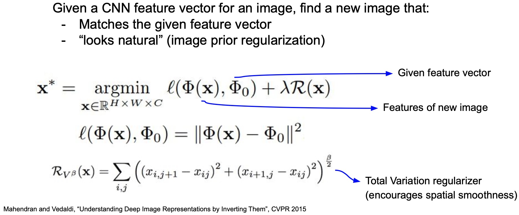
- Shown above – this is what the \(argmin\) function is trying to do – it’s taking an input image \(X\) and passing it through your network.
- Let’s say that you have the features from, say, Conv5 and we represent that as \(\phi_0\). So \(\phi_0\) is some cached representation of an image that we have already featurized at some point in the past, but we’ve lost the image.
- We start off with a random \(x\) and forward-pass it through our network to calculate \(\phi_0\), the Conv5 features. Our goal is to recreate an image \(x\) that minimizes the difference between (i) the features predicted by our network for this image and (ii) the cached features that we already have, using an L2-norm.
- Simply put, we’re trying to figure out exactly what is the \(x\) that minimizes this formulation.
- We’ve talked about different regularization techniques. Here’s one that specifically helps the case of generating realistic images, called the total variation regularizer. What the total variation regularizer is trying to capture:
- Intuitively, what it’s doing is that it’s smoothing out the pixels spatially. In other words, it encourages spatial smoothness.
- It’s basically saying if 2 pixels are close together spatially, they must have the same value.
- This is generally true of the world as we look around – nearby pixels do have similar values.
- Using this formulation, can we recreate our images? Turns out we can!
Note that this has implications in privacy, because a lot of people were releasing datasets where we would featurize videos and images, hoping that those would be secure and you wouldn’t be able to get back the original images from which those features came from. With feature inversion, that is no longer true! We can’t just release our features because we can in fact recreate the original source that they came from.
- Here are examples of what happens when you recreate these 2 specific images from different layers of a VGG-16:
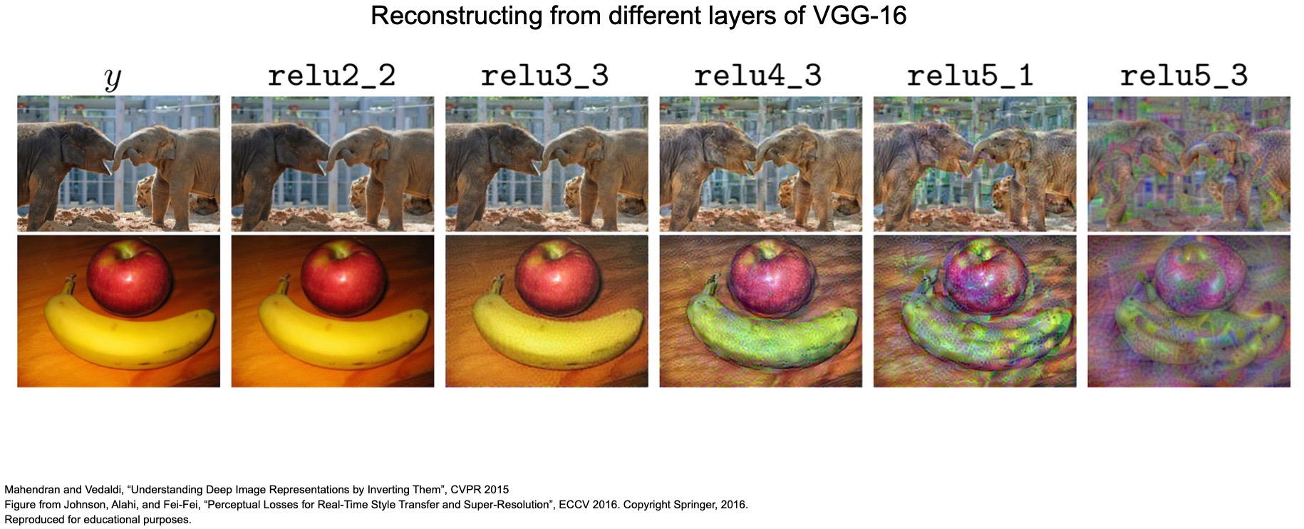
- If you try to recreate your images after the second layer, ReLU2, you can almost recreate it perfectly. But the further you go into the model and try to recreate it, the harder it becomes, because the further your features are in your network the more high-level those features are.
- Recall that we’ve talked about how the the the lower layers often characterize textures, colors and blobs but the later layers are capturing these high-level features or semantic meanings of what’s in an image by characterizing its shape, so they often forget about the texture and colors.
- If you try to recreate your image from say, Conv5 or ReLU5, those actually end up looking not so great but they do still have the general sort of shape of the kinds of things you would typically expect for that given image.
- You can still kind of make out a banana and an apple or the two elephants but it has lost a lot of its textures and colors in that process.
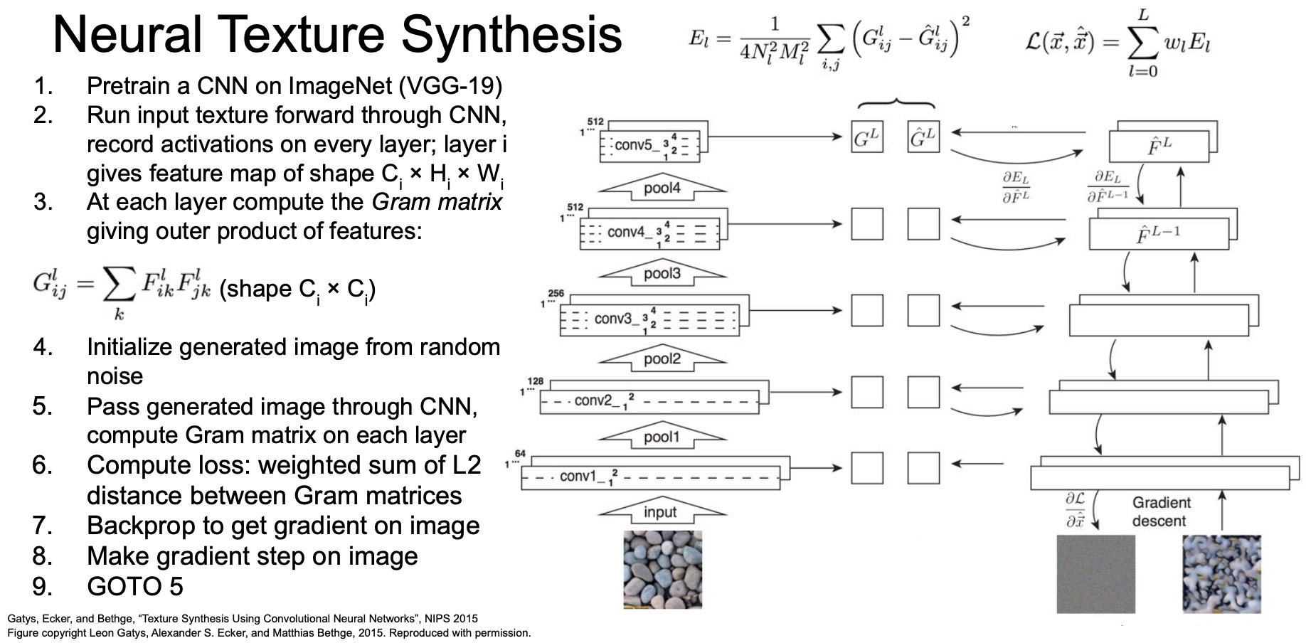
Texture Synthesis
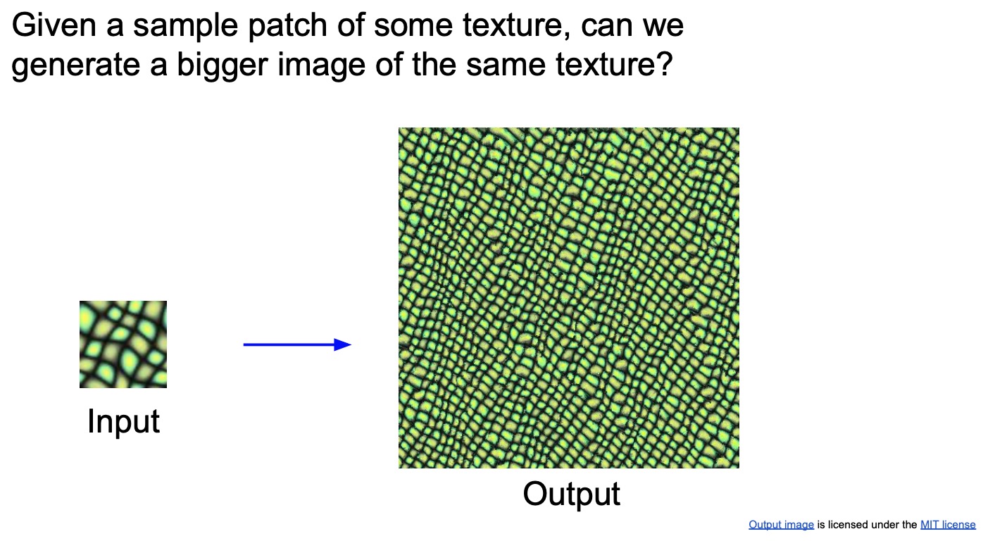
- The idea of synthesizing texture is one that has been widely studied across many many decades at this point in computer graphics.
- There’s a lot of work in the pre-deep learning era where they’ve been taking input textures and building models that can replicate this texture. We’ve been borrowing techniques like this from computer graphics and applying them in computer vision tasks. Generally these methods work very well with simple textures and don’t really need neural networks.
- “Fast Texture Synthesis using Tree-structured Vector Quantization” (2000) by Wei and Levoy is a simple algorithm from the pre-deep learning era.
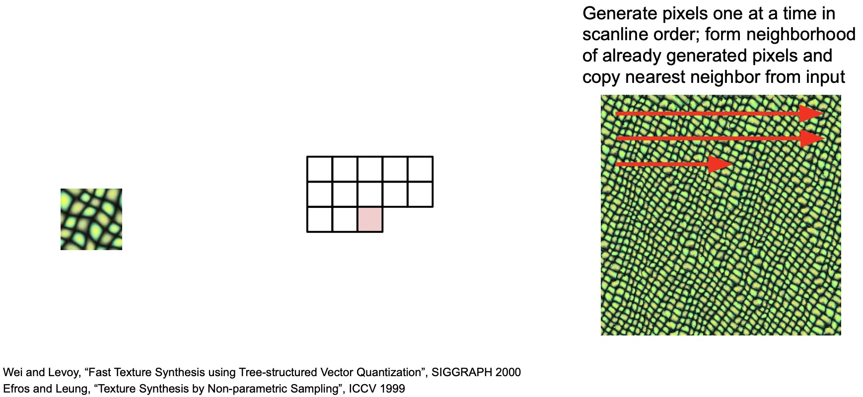
- The general idea texture synthesis is that you take an input texture and figure out ways in which you can synthesize it for a larger geometric region in a way that makes it seem natural.
- Of course, texture synthesis methods are not perfect – consider this example of generating a brick wall (shown below), it doesn’t look realistic because if bricks come out to be different sizes. Similarly, if you try to replicate words, and if you zoom in, you’ll notice that they don’t actually represent letters, so it doesn’t work very well. However, if you look at it from afar, the texture does kind of make sense. Thus, simple algorithms don’t work well with complex textures!
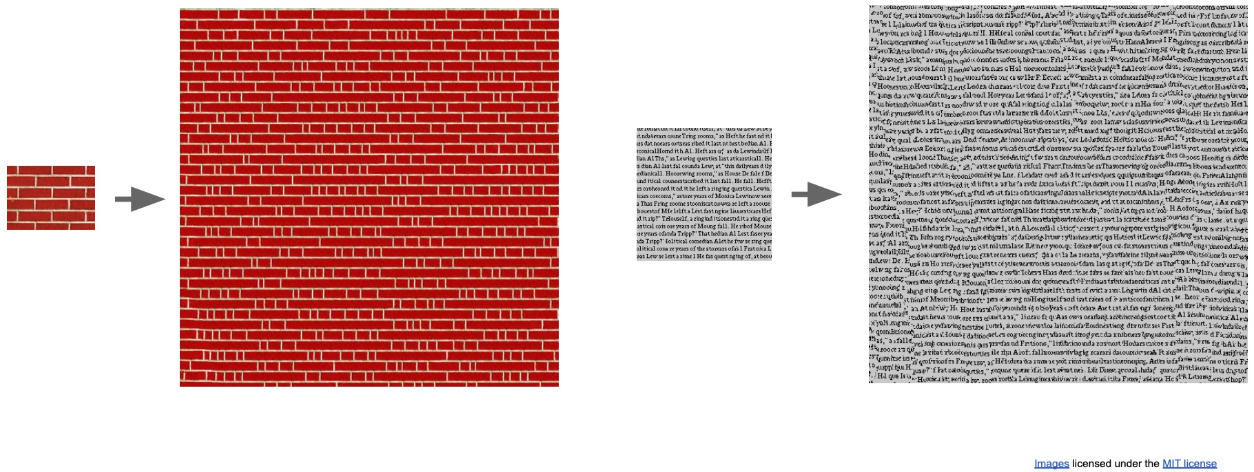
- Overall, this idea of texture synthesis was very exciting to a lot of people in computer vision as well. We started thinking about what are ways in which we can use the deep learning techniques we have today to improve these feature inversion methods that we’ve been discussing about. How can we actually recreate our images from these high-level feature representations and still retain these kinds of textures that we want to have?
- To retain texture there’s this idea that it came out called the gram matrix.
Gram Matrix
- The gram matrix is a matrix that represents some high dimensional representation of the kinds of features do not expect to have in a texture that you care about.
- Let’s say that the texture we want to replicate is this image of stones:
- Steps to generate an element in a gram matrix (shown in the figure below):
- Get a pre-trained network.
- Run an input image (in our particular case, images of stones) through it.
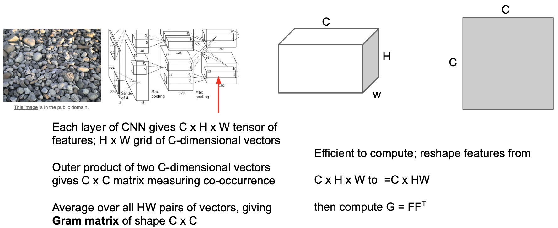
- Extract representations/activations of a particular layer, say Conv5.
- These activations take the shape of \(C \times H \times W\) where \(H\) and \(W\) are your spatial extents and \(C\) is your channel depth.
- Take the dot product of these representations and any pair of spatially located vectors.
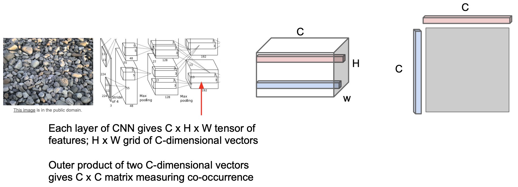
Intuitively, the gram matrices are capturing some amount of co-occurrence between feature vectors at different spatial locations. In other words, it’s distilling some sort of second order statistic of what’s contained in that texture.
- Note that gram matrices do not depend on \(H\) or \(W\), they just depend on your channel width. Ultimately, because the grand matrix is a \(C \times C\) matrix because you multiply out all the pairs of values in the spatial dimensions. It’s pretty easy to actually compute the gram matrix, which is why a lot of people use it.
- The correct way to really think about co-occurrences between different vectors is using a covariance matrix (similar to what we saw in PCA) but covariances are really costly to compute. Covariances are really useful in understanding the different features that are captured or represented in our image, but they’re really expensive to calculate.
- Gram matrices are this effective, less compute intensive way of calculating these second order statistics that are by all means just an approximation but they tend to work really well.
- To calculated your gram matrix, you reshape your activation from \(C \times H \times W\) such that it’s just \(C \times HW\) and then you just multiply it by its transpose to get your \(C \times C\) matrix, as shown in the figure below.
Neural Texture Synthesis with Gram Matrix
- The “neural texture synthesis” line of work tackles the problem of generating realistic textures (better than classical computer graphics techniques) using deep learning.
- To generate realistic textures using the concept of a gram matrix:
- Take the input texture image (say, the rocks shown above), pass it through our ImageNet-pre-trained network. Get gram matrices \(G_1^l\) at different layers from this network.
- Take another network that we’re going to train. Start off with an image initialized from random noise. Generate gram matrices \(G_2^l\) at every layer.
- Backprop the losses in this network using an L2-loss such that the gram matrices between all of these pairs \(G_1^l, G_2^l\) are close together at every single layer of our network.
- Backprop to our input image until eventually we produce an image that matches the gram matrices of the texture we care about.
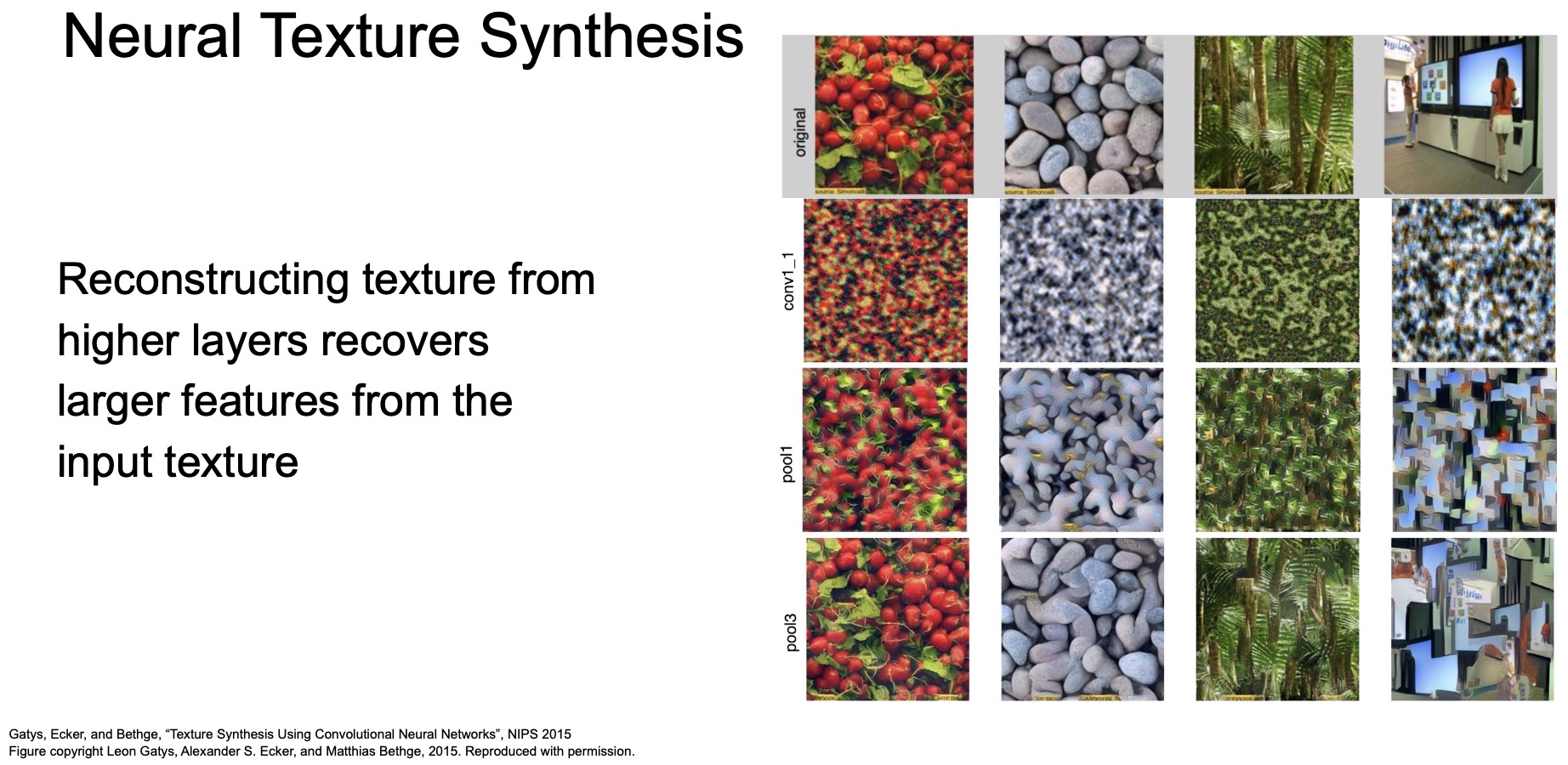
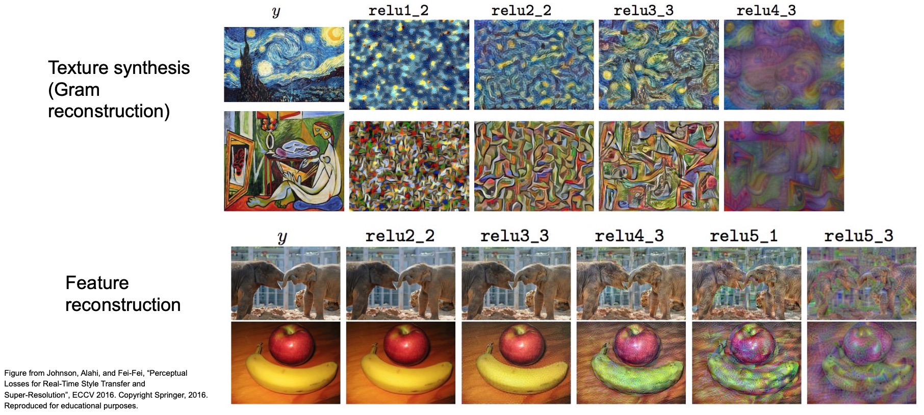
You see a similar pattern emerge as earlier (shown below), where depending on which gram matrix you choose from which layer, you get back different kinds of textures. If you use the later/higher layers, you retain more of the high-level shapes of objects, but using the earlier/lower layers retains more of the textures and color blobs so it’s a trade-off where you might want to think about exactly which gram matrices at which layer are the most important for your given task.
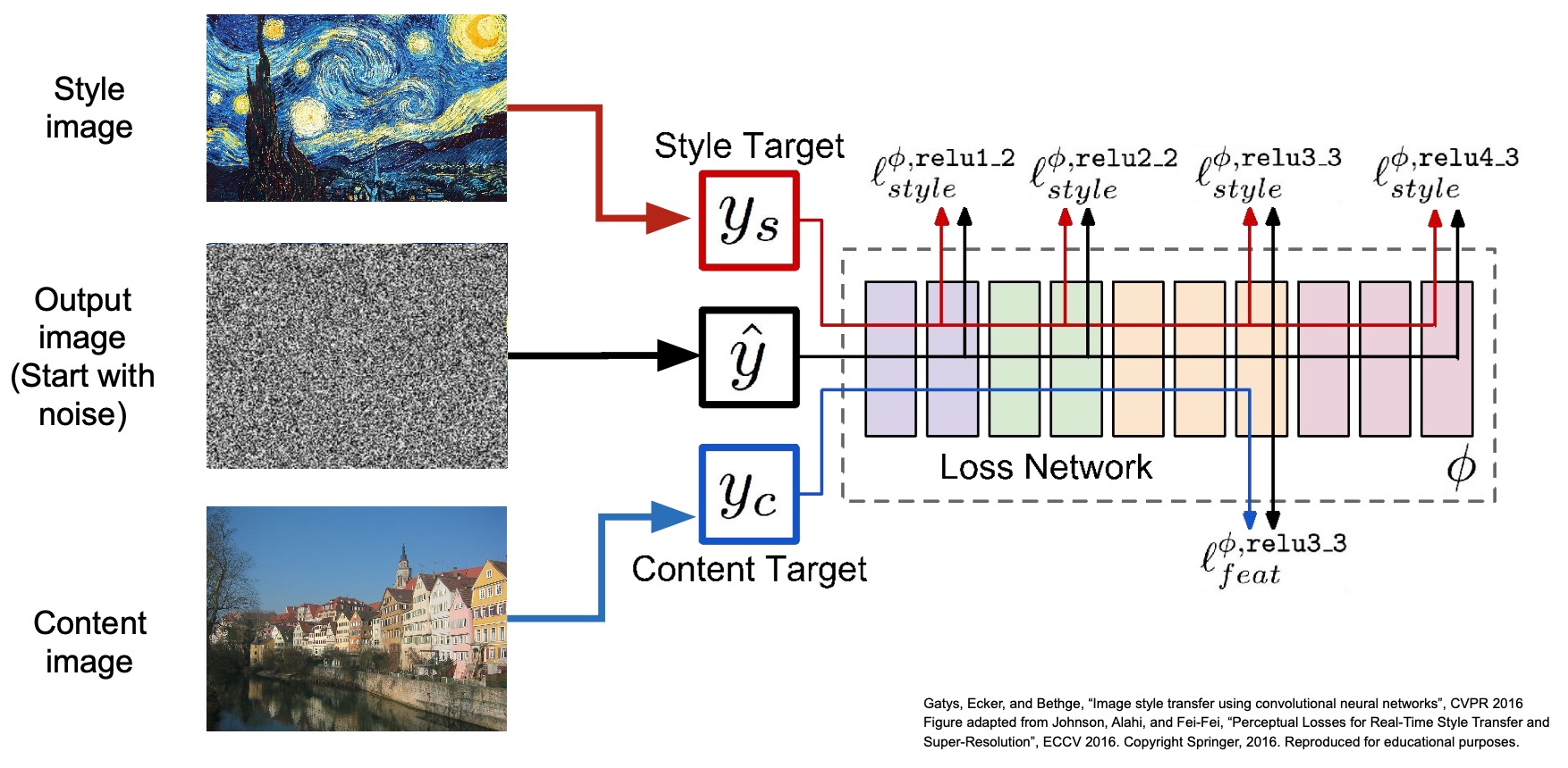
Neural Style Transfer: Feature Inversion + Gram Matrices
- A similar idea can be applied to artwork generation as well.
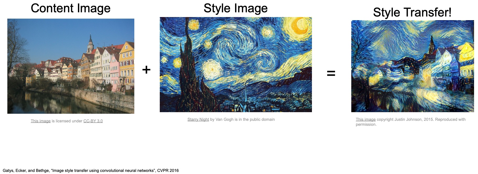
- Take a Van Gogh Starry Night image as our “style” reference and then try to recreate other images by retaining their “content” but using the same “style”, i.e., the kind of textures that our “style” reference contains.
- Let’s juxtapose the ideas of Feature Inversion and Gram Matrices together. Recall the roles of each of these two concepts:
- Feature inversion: to get back the original contents of an image from a feature.
- Gram matrices: allow us to distill the textures/style in an image.
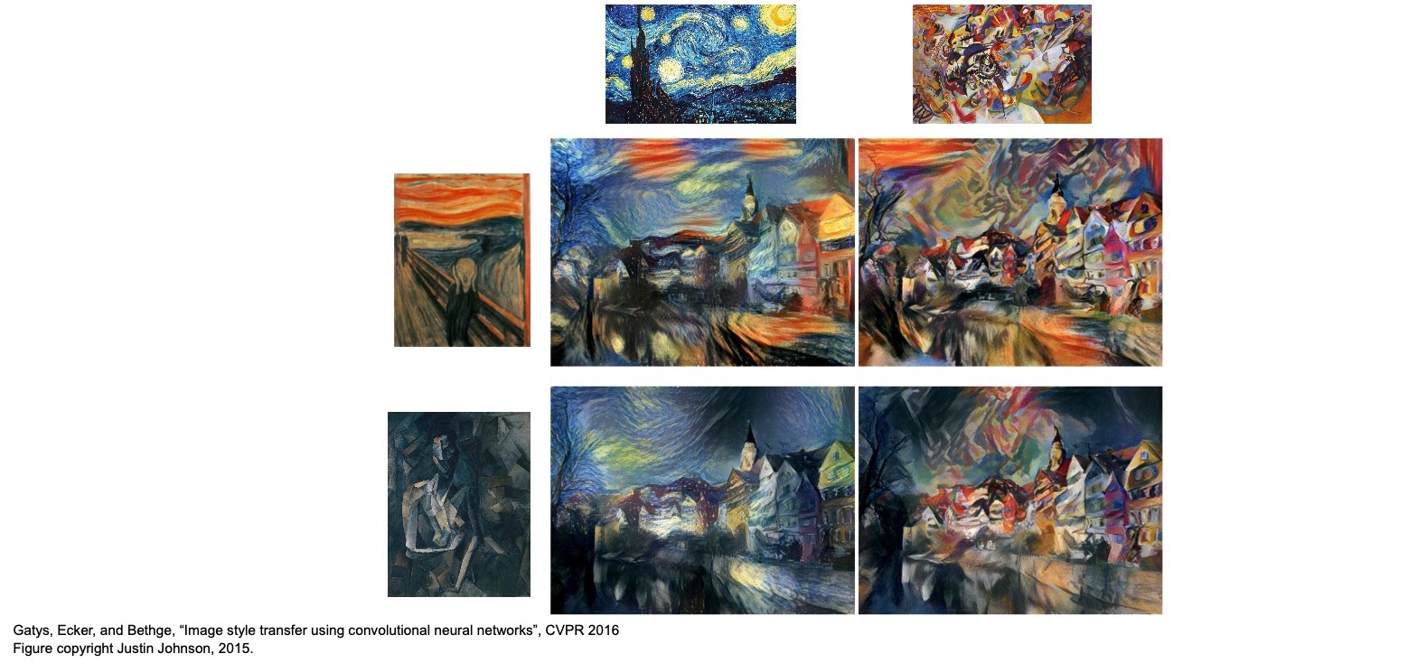
- In “A Neural Algorithm of Artistic Style” (2016), Gatys et al. proposed taking a content image and style image and putting them together such that we can create images that have the content from our content image and the textures and style from our style image. This field of research is called Neural Style Transfer.
- Steps to carry out Neural Style Transfer:
- Input an image generated using a random noise vector to a network pre-trained on ImageNet (the original paper used VGG).
- As part of training, seek to minimize the gram matrices loss with respect to the style image and the feature representations of the content image.
- Perform gradient ascent during backprop until you obtain your desired output.
In the below diagram, note that since the earlier layers of the network capture much of the colors, blobs and textures, they are adept at representing the style of the image (which is why we prefer to extract the style from the initial layers), whereas the later layers of the network capture the shape and thus, represent the content (which is why we use the later laters to extract the content of the image).
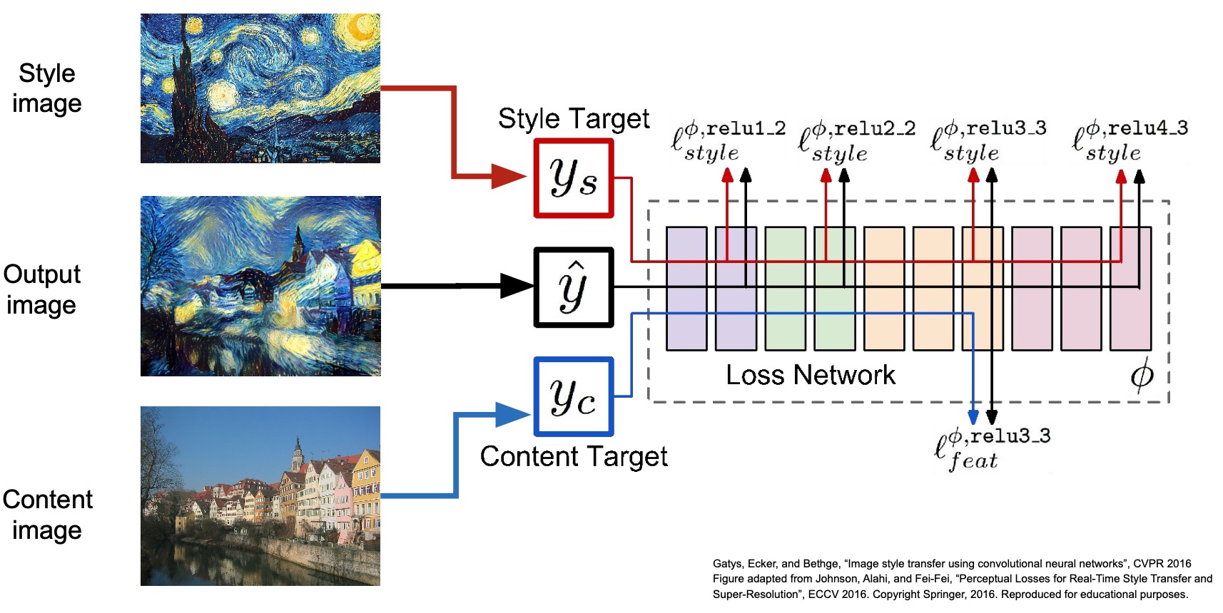
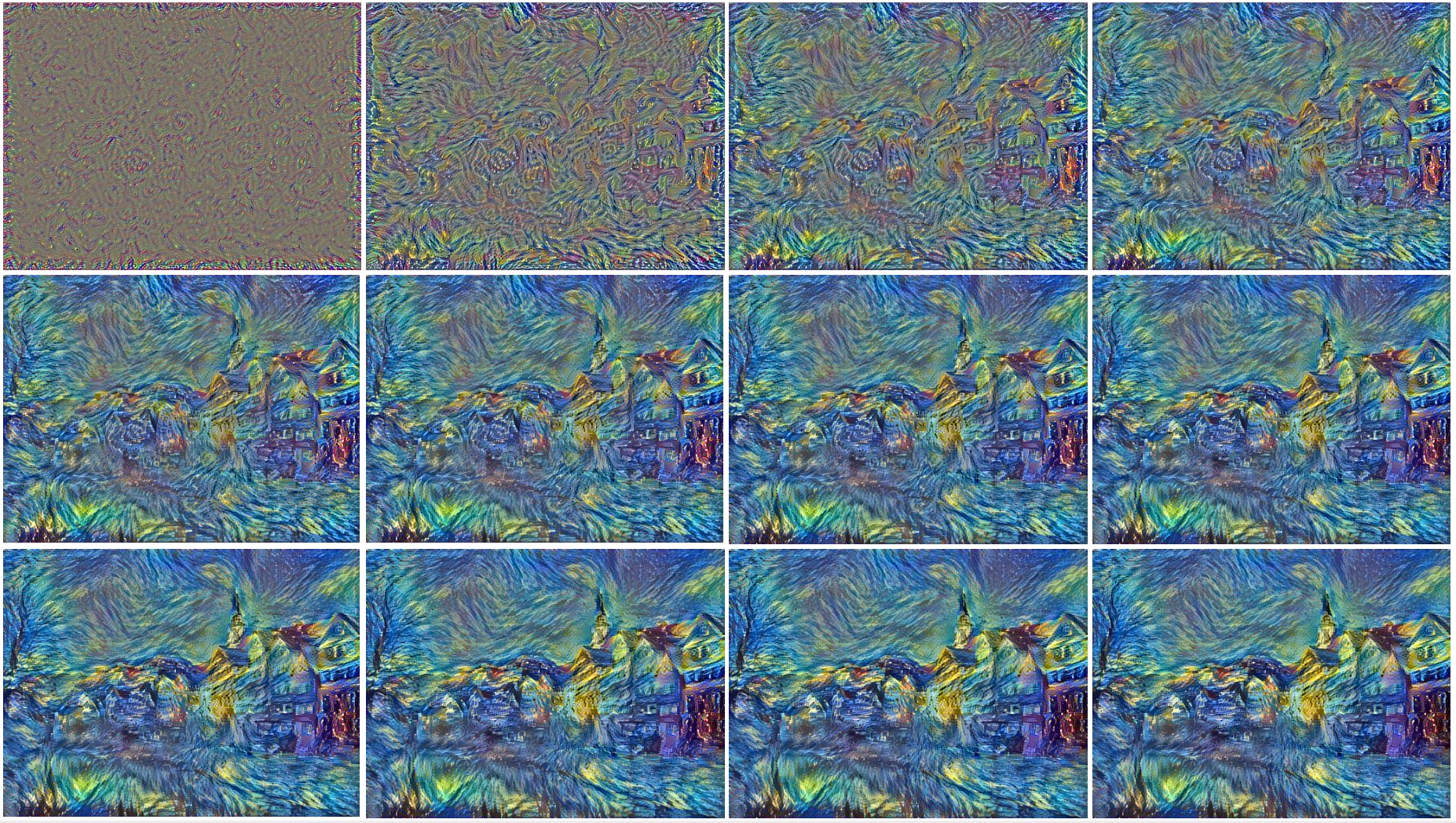
- Shown below is the graphical process of neural style transfer (shown with an iteration-step of 100). As seen below, you need to backprop into the noisy input image for a decently large number of iterations before you see glimpses of your expected output. The number of iterations to backprop is usually a hyperparameter.
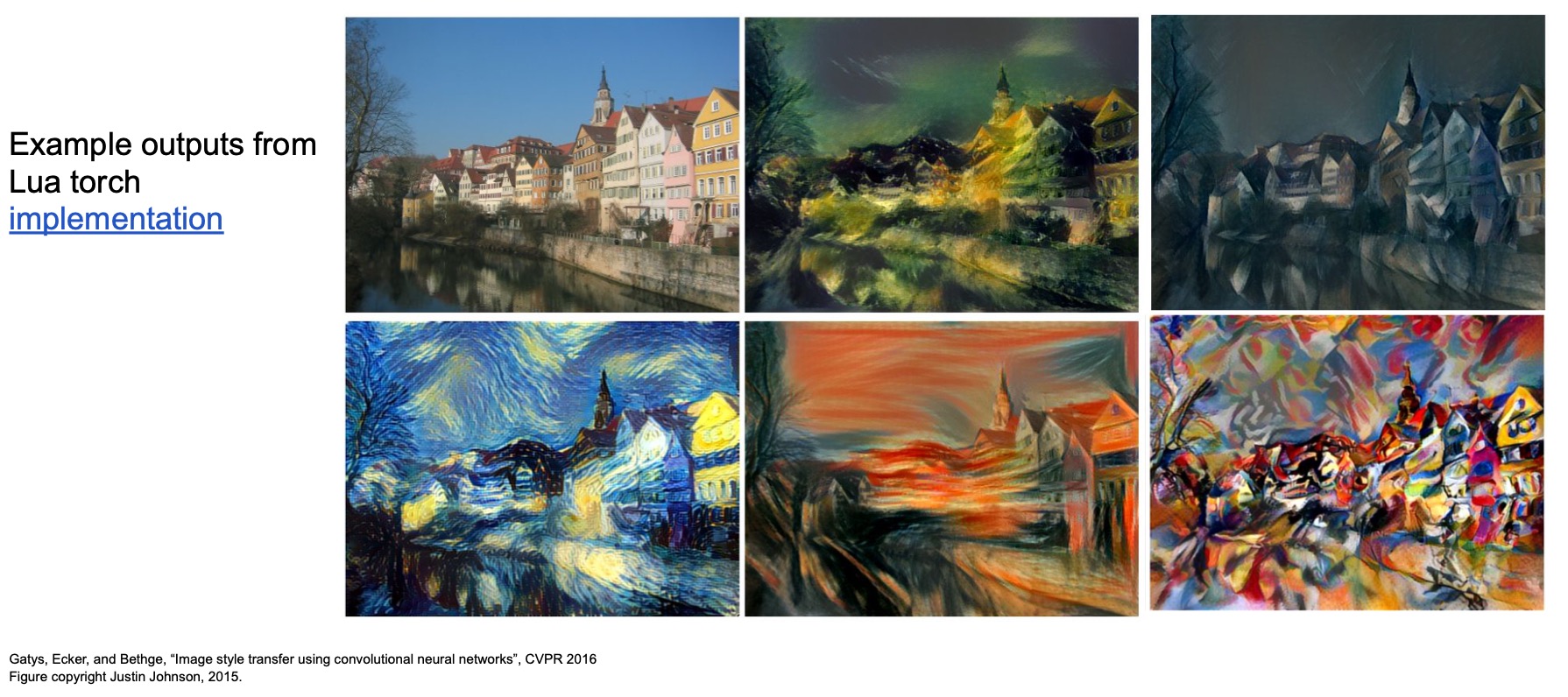
- There are implementations of it available online (lua + PyTorch). Shown below are some examples of generated artwork.
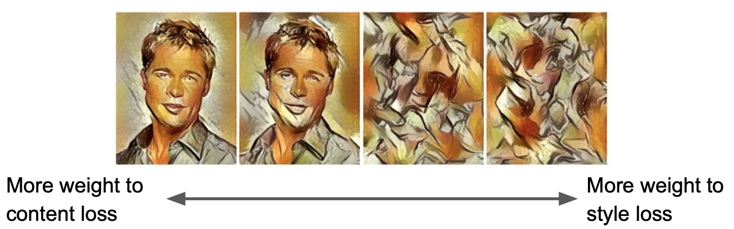
- Recall the trade-off we discussed between the content loss and the style loss, where you need to figure out exactly how to weigh these two components when combining them together to formulate your overall loss (similar to RNNs, where you accumulate your loss at every single time-step to form your overall loss). If you weigh style loss heavily, you’ll get the textures but no content. On other hand, if you weigh the content loss heavily, you’ll just get the content and not much of the style. Shown below are examples of images that you can generate, depending on how you trade-off content versus style.
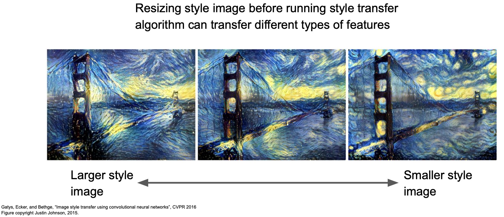
- Similarly, there’s a trade-off between using smaller or larger style images as well.
- Multiple style images can also be used by taking a weighted average of Gram matrices:
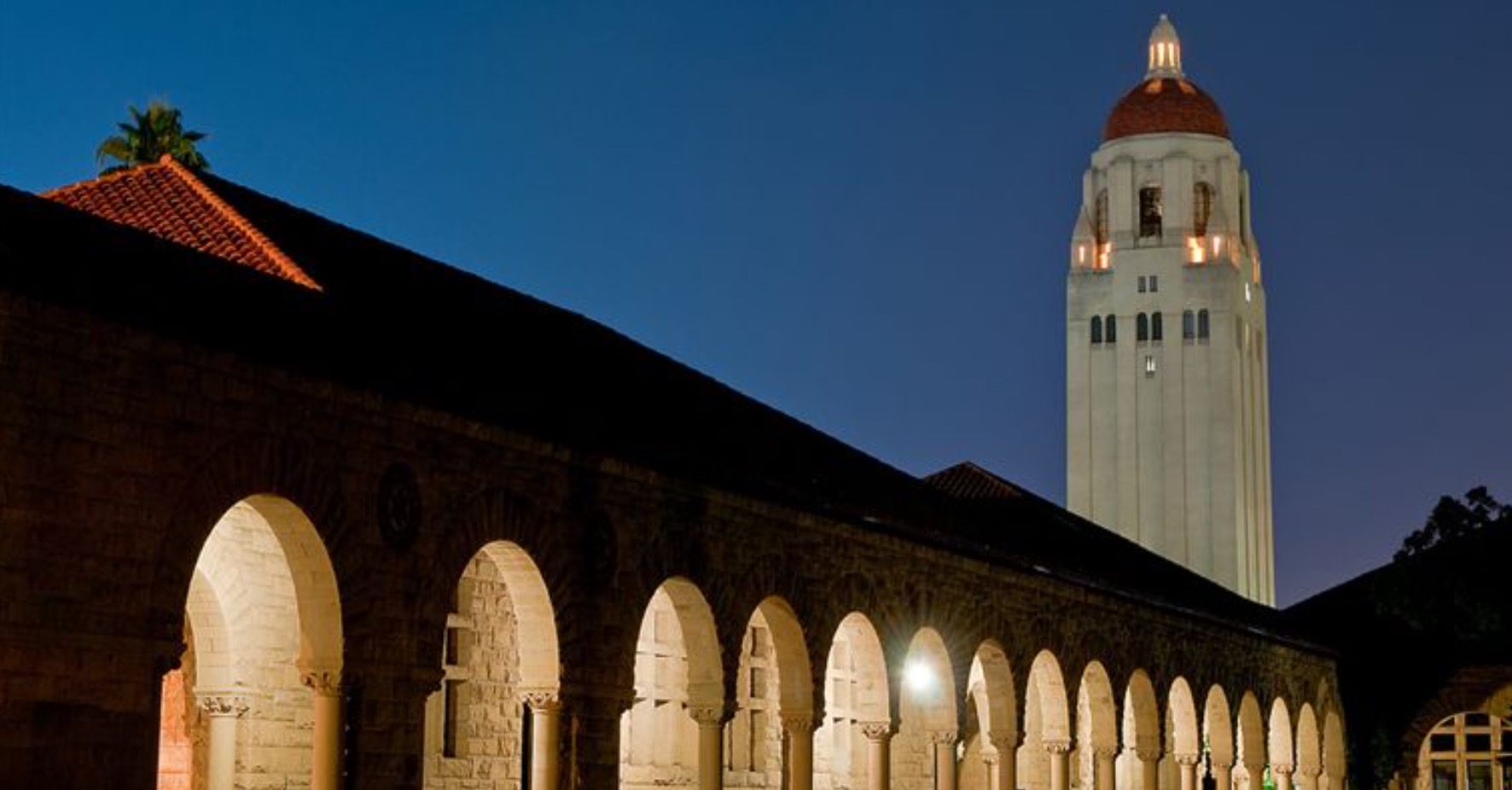
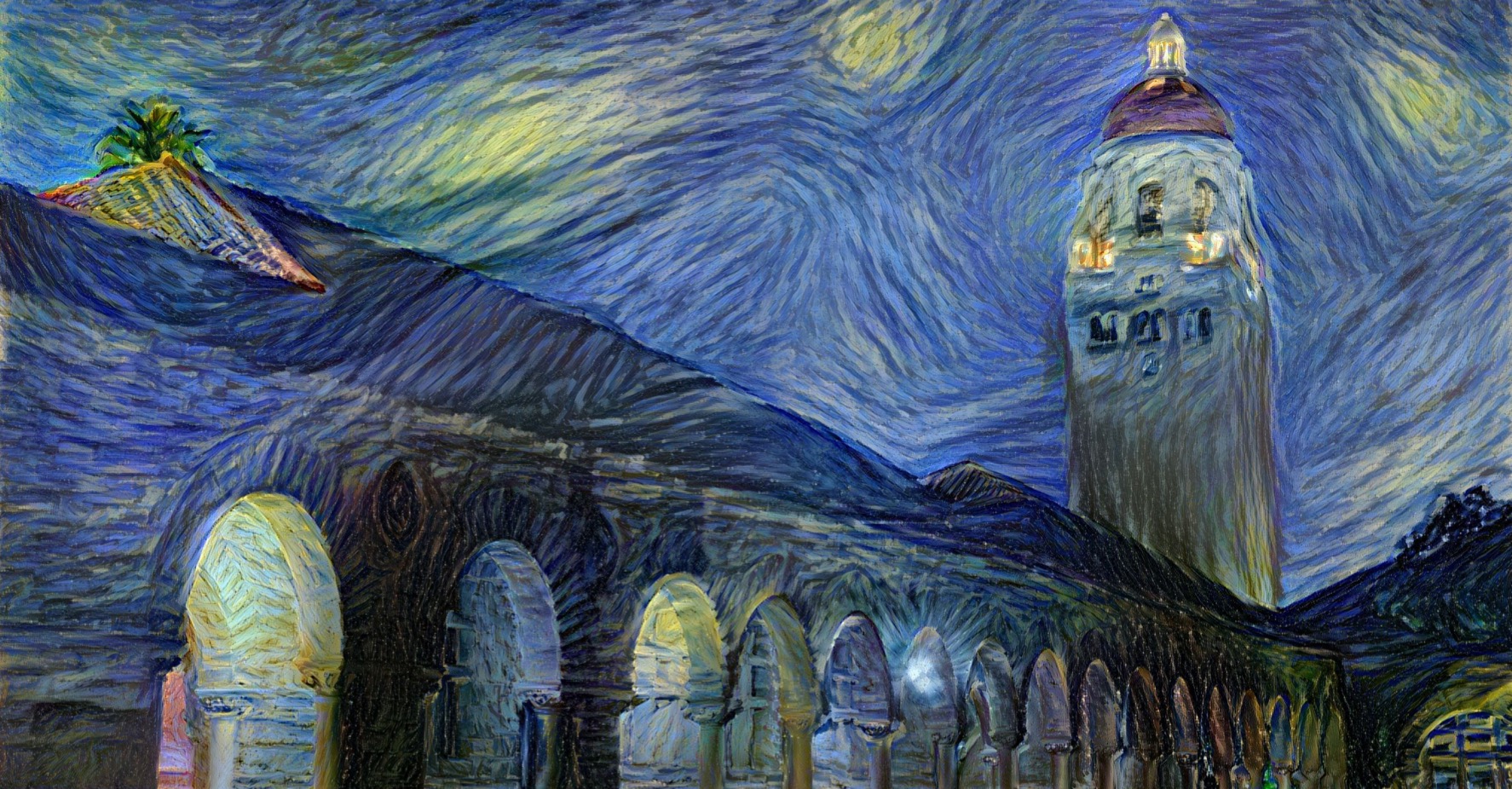
- Applying Starry Night using neural style transfer to the Hoover tower at Stanford:
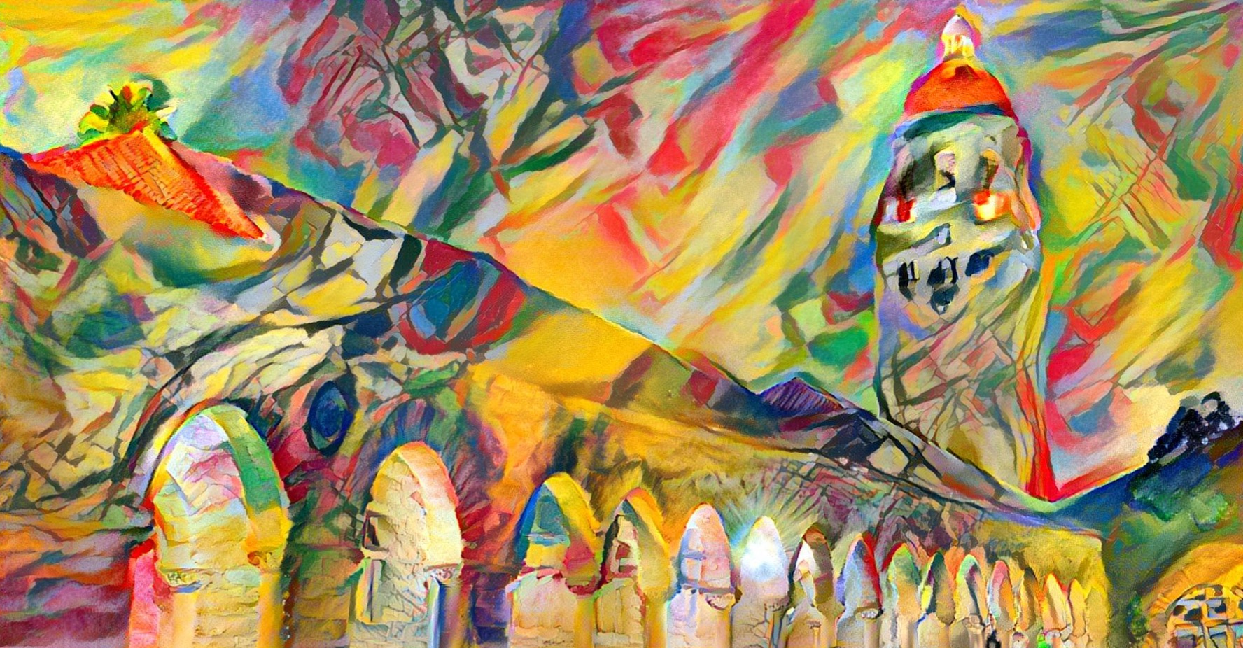
- Another style:
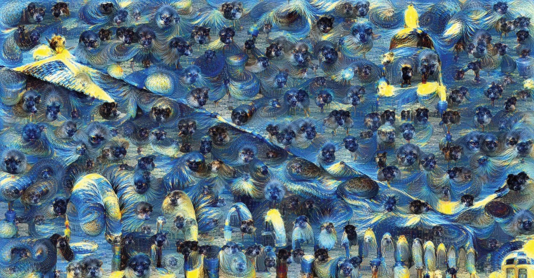
- Even add deep-dream on top of it, to make it look like there are dogs overlayed on top!
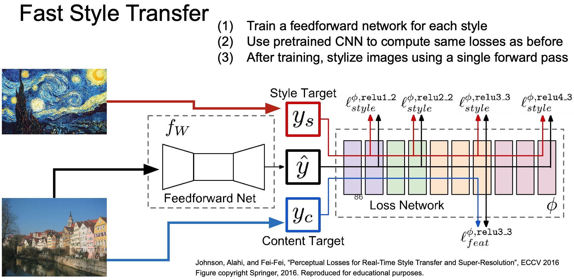
Fast Style Transfer
- The problem with neural style transfer is that it requires many forward/backward passes through the pre-trained VGG network, needs several gradient ascent update steps to achieve our desired end-product and is thus very slow.
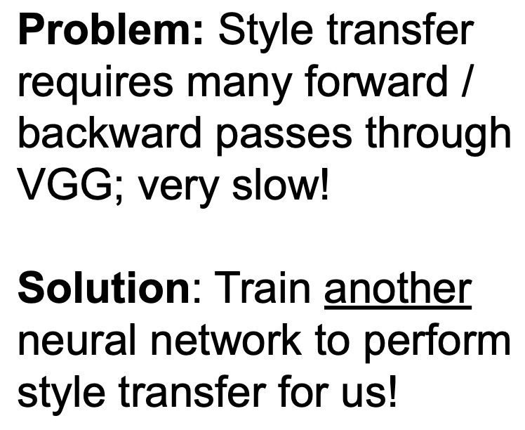
- Solution: Fast style transfer. Train another network to generate a style transferred-image automatically!
- Fast style transfer basically tries to make the process of stylizing images quicker and figures out how to do this without using too many gradient ascent update steps.
- Fast style transfer accomplishes this using the following steps:
- Train one network for a particular style
- Compute similar gram matrices-based losses as before using a pre-trained CNN, say VGG.
- Instead of back propagating to an empty image, you’re training a feed-forward network’s weights.
- The reason this is called a feed-forward network is because during the backward pass, you do not perform backprop on it using its own forward pass, but instead use the forward pass of the pre-trained network to come up with your loss (and hence your gradients).
- Once training is done, you can stylize your images with the particular style your network was trained on using a single forward pass.
- Some examples of images generated using fast style transfer:
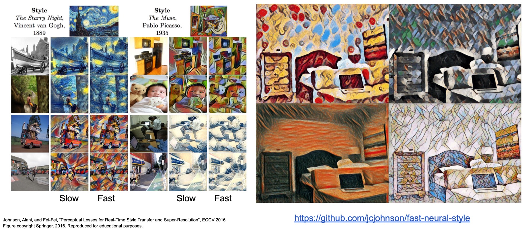
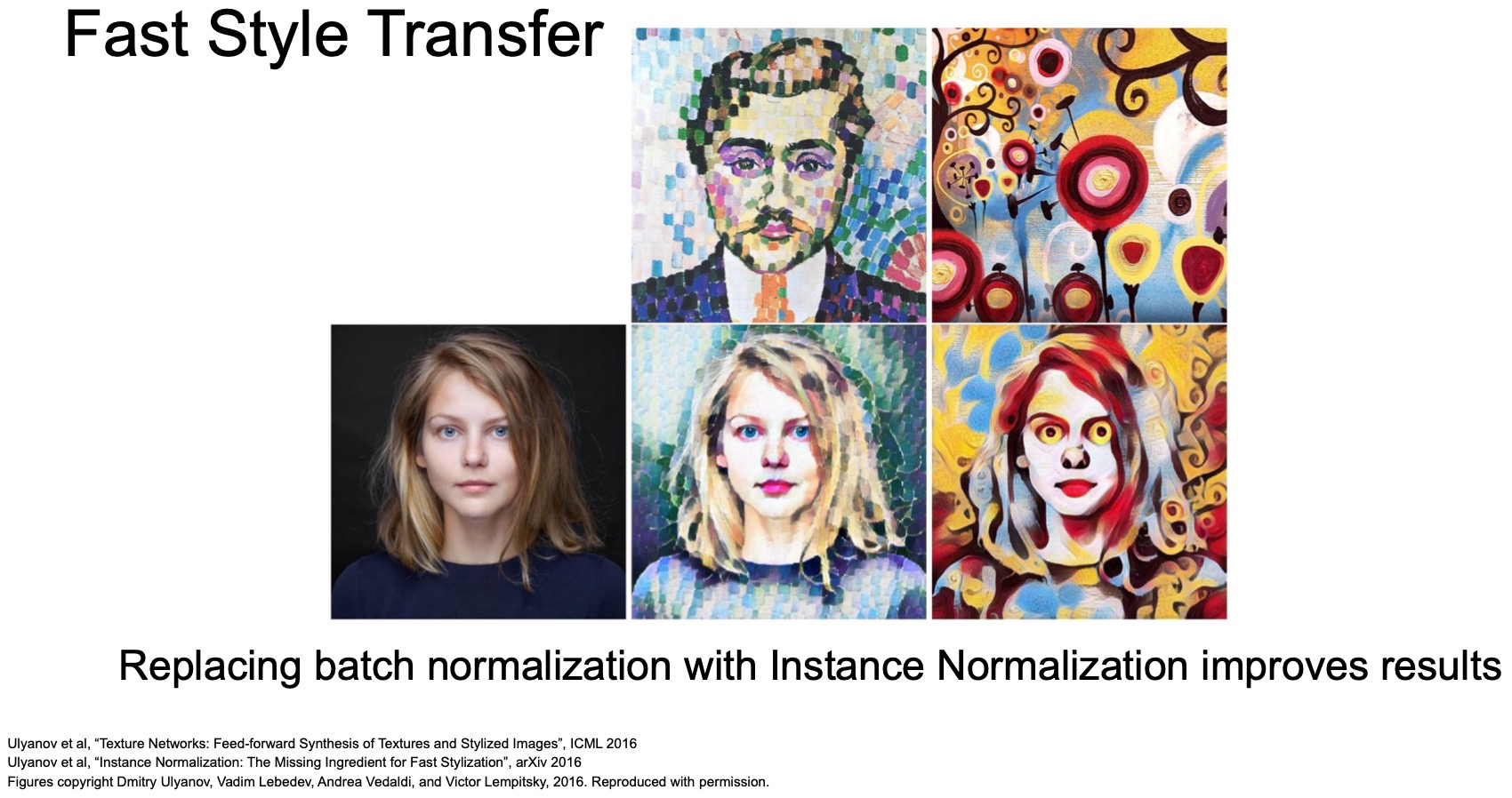
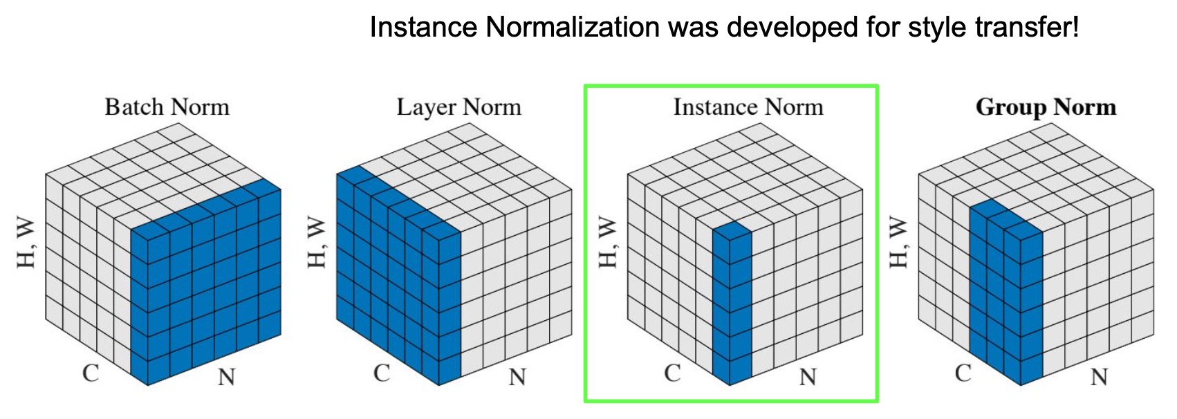
- In “Perceptual Losses for Real-Time Style Transfer and Super-Resolution” (2016), Johnson et al. proposed using perceptual losses instead of pixel-wise L1/L2-distance based loss to improve training time. Similarly, they proposed using Instance Normalization (which was developed to improve Style Transfer training) to significantly improve training convergence times.
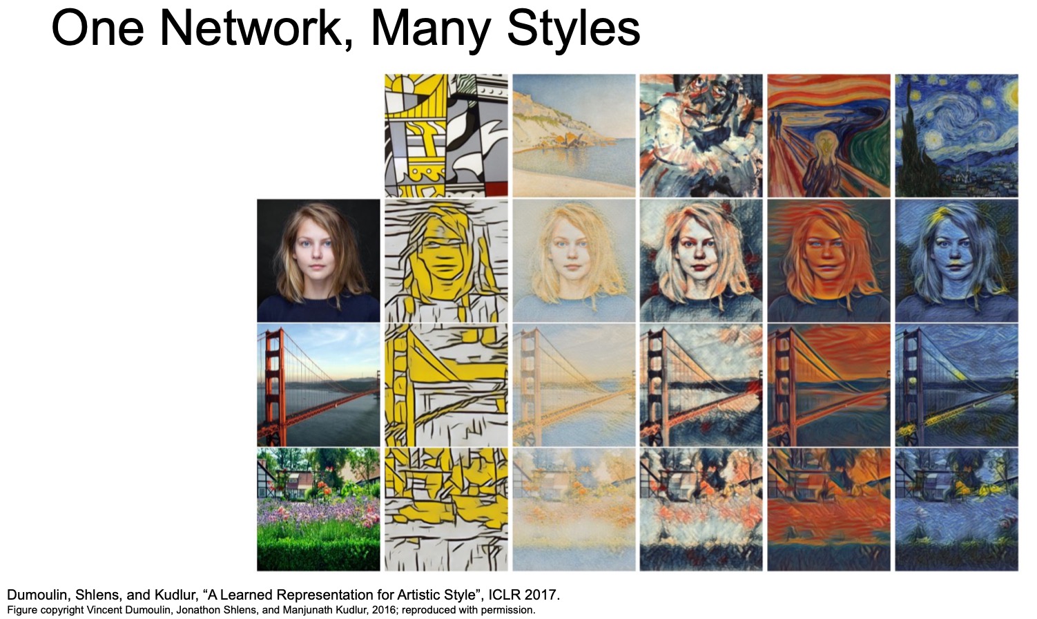
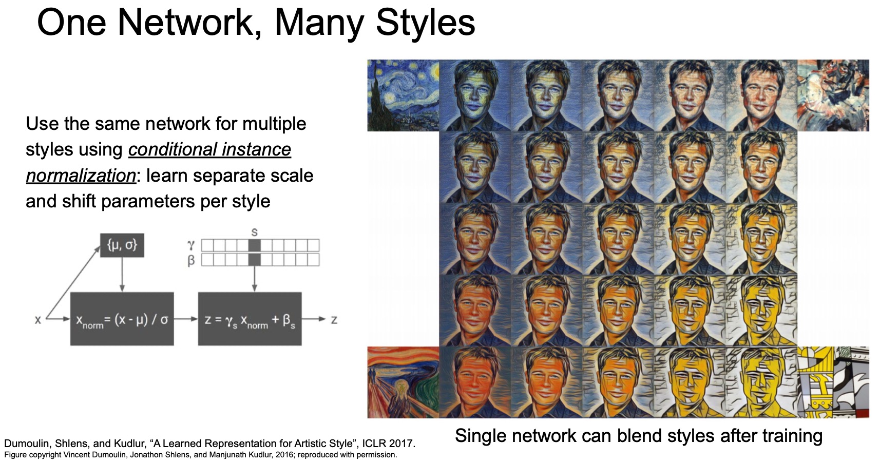
- There’s been a lot of follow-up works in the area of style transfer. In “A Learned Representation For Artistic Style” (2017), Dumoulin et al. proposed having one network that’s trained to do different kinds of styles, so it’s a really exciting line of work as well that is actively being worked on even today in computer vision.
Key Takeaways
- We talked about methods for visualizing and understanding CNN representations.
- Visualizing activations: understanding them by applying nearest neighbors on a 4096-D FC layer feature vector, dimensionality reduction techniques (PCA, t-SNE) to understand the geometry of this space that’s learned, maximally activating patches.
- Visualizing gradients: saliency maps using occlusion, saliency maps using backprop, different kinds of class visualizations, adversarial learning, fooling images, feature inversion.
- Fun techniques: finally, we clubbed the ideas of feature inversion and texture extraction using gram matrices and showed that you can build techniques like neural style transfer, DeepDream.
Further Reading
Here are some (optional) links you may find interesting:
- Receptive field to learn about the concept of receptive field and effective receptive field.
- Introduction to t-SNE to learn implementation details about t-SNE.
- Adversarial Examples and Adversarial Training to learn more about this adversarial training and examples.
- Coursera-NLP | Word Embeddings and Vector Spaces for implementation details of PCA.
Citation
If you found our work useful, please cite it as:
@article{Chadha2020DistilledVisualizingUnderstanding,
  title   = {Visualizing and Understanding},
  author  = {Chadha, Aman},
  journal = {Distilled Notes for Stanford CS231n: Convolutional Neural Networks for Visual Recognition},
  year    = {2020},
  note    = {\url{https://aman.ai}}
}