Primers • Chain Rule

• Motivation
• Chain rule
• Chain rule in the context of computational graphs

Motivation

• To understand the channeling of the gradient backwards through the layers of your network, a basic understanding of the chain rule is vital.

Chain rule

• If \(f(x)=g(h(x))\) and \(y=h(x)\), the chain rule can be expressed as,

  • Using Leibniz’s notation,
  \[\dfrac{\mathrm{d}f}{\mathrm{d}x} = \dfrac{\mathrm{d}f}{\mathrm{d}y} \cdot \dfrac{\mathrm{d}y}{\mathrm{d}x}\]
  • Using Lagrange’s notation, \(\dfrac{\mathrm{d}f}{\mathrm{d}y} = f’(y) = f’(h(x))\) and \(\dfrac{\mathrm{d}y}{\mathrm{d}x}=h’(x)\),
  \[\therefore f'(x)=f'(y)\,h'(x)=f'(h(x))\,h'(x)\]

• It is possible to chain many functions. For example, if \(f(x)=g(h(i(x)))\), and we define \(y=i(x)\) and \(z=h(y)\), then,

• Using Lagrange’s notation, we get,

• The chain rule is crucial in Deep Learning, as a neural network is basically as a long composition of functions. For example, a 3-layer dense neural network corresponds to the following function (assuming no bias units):

  \[f(X)=\operatorname{Dense}_3(\operatorname{Dense}_2(\operatorname{Dense}_1(X)))\]
  • In this example, \(\operatorname{Dense}_3\) is the output layer.

• Generally speaking, assume that we’re given a function \(f(x, y)\) where \(x(m, n)\) and \(y(m, n)\). The value of \(\frac{\partial f}{\partial m}\) and \(\frac{\partial f}{\partial n}\) can be determined using the chain rule as:

Chain rule in the context of computational graphs

• The figure below summarizes the use of the chain rule for the backward pass in computational graphs.

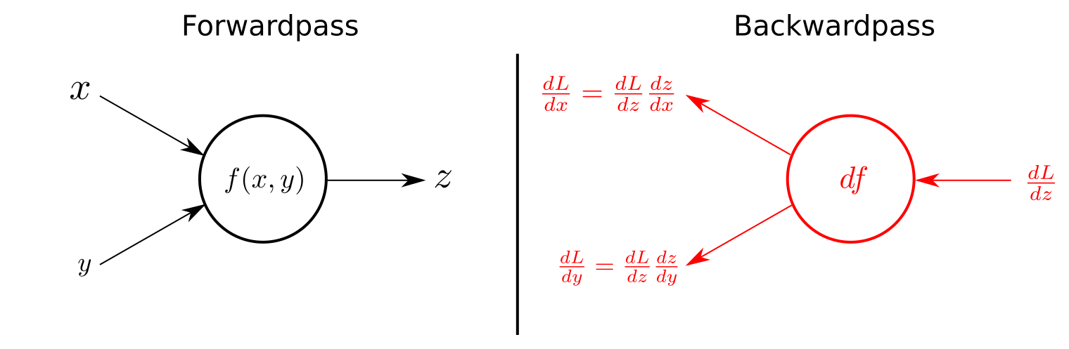
• In the figure above, the left-hand-side of the figure illustrates the forward pass and calculates \(z = f(x,y)\) using the input variables \(x\) and \(y\).
  • Note that \(f(\cdot)\) could be any function, say an adder, multiplier, max operation (as in ReLUs) etc. Gradient routing/distribution properties of standard “gates” along with the derivatives of some basic functions can be found in Stanford’s CS231n course notes.
  • Note that the variables \(x\) and \(y\) are cached, which are later used to calculate the local gradients during the backward pass.
• The right-hand-side of the figure shows the backward pass. Receiving the gradient of the loss function with respect to \(z\), denoted by \(\frac{dL}{dz}\), the gradients of \(x\) and \(y\) on the loss function can be calculated by applying the chain rule as shown below.

• Generally speaking, the chain rule states that to get the gradient flowing downstream, we need to multiply the local gradient of the function in the current “node” with the upstream gradient. Formally,