Aman's AI Journal • Coursera-NLP • Word Embeddings and Vector Spaces

Vector space models
Word by word design
Word by document design
Euclidean distance
Cosine similarity
Word manipulation in vector spaces
PCA
Document as a vector
Further reading
Citation

Vector space models

Suppose you have two questions: "Where are you heading?" and "Where are you from?". Note that these sentences have identical words, except for the last ones. However, they both have a different meaning, as shown in the left-hand-side of the figure below.
On the other hand, say you have two more questions whose words are completely different but both sentences mean the same thing, as shown in the right-hand-side of the figure below.

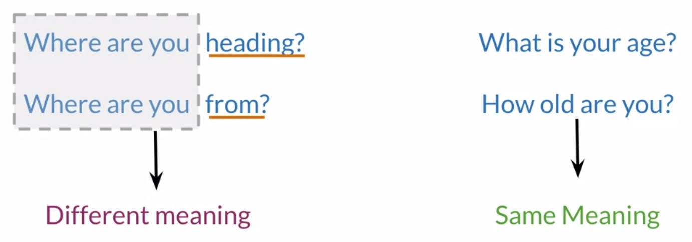
Vector space models help you identify whether the first pair of questions or the second pair are similar in meaning even if they do not share the same words. Similarity identification has applications in question answering, paraphrasing, and summarization.
Vector space models also allow you to capture dependencies between words by representing words as vectors, referred to as word vectors/vector representations of words/word embeddings.
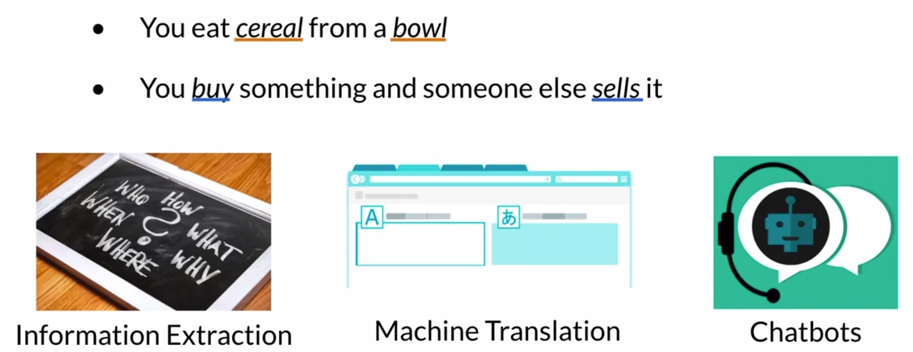
- Consider the sentence: "You eat cereal from a bowl". Here, you can see that the word cereal and the word bowl are related.
- Now let’s look at this other sentence: "You buy something and someone else sells it". What the sentence is saying is that someone sells something because someone else buys it. The second half of the sentence is dependent on the first half.
With vector space models, you can capture relationships among different sets of words. Vector space models are used in information extraction to answer questions in the style of who, what, where, how, etc. – which have applications in information extraction, machine translation and chatbots.

John Firth, a famous English linguist, once said: "You shall know a word by the company it keeps". This is one of NLP’s most fundamental concepts. When using vector space models, the way that representations are made is by identifying the context around each word in the text, and this captures the relative meaning.

Key takeaways
- Vector space models enable representing words in text documents like tweets, articles, queries, or more generally, an object that contains text, as a vector.
- Since these word vectors capture relative meaning by identifying the context of the word, they lend themselves to applications where similarity identification is of essence. This includes the fields of information retrieval, indexing, relevancy ranking, information filtering etc.
  - For e.g., when you look up a query online, the algorithm relies on the above concepts to give you back your results.
- NLP fundamental concept: "You shall know a word by the company it keeps" - Firth, 1957.
- Applications include:
  - Information Extraction
  - Machine Translation
  - Chatbots

Word by word design

Let’s delve into how you can construct word vectors from scratch using a co-occurrence matrix. Depending on the task at hand that you’re trying to solve, you can have several possible designs.
To get a vector space model using a word by word design, you’ll compute a co-occurrence matrix and extract vector presentations for the words in your corpus.
The co-occurrence of two different words is the number of times that they appear in your corpus together within a certain word distance \(k\).
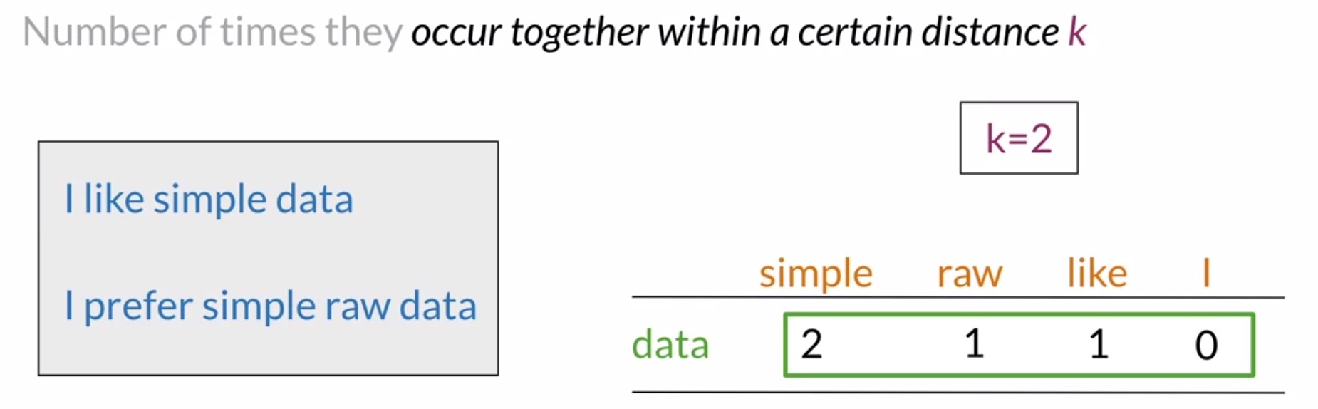
- For instance, suppose that your corpus has the following two sentences: "I like sample data" and "I prefer simple raw data".
- The row of the co-occurrence matrix corresponding to the word data with \(k = 2\) would be populated as shown in the figure below.
- For the column corresponding to the word simple, you would get a value equal to 2 because data and simple co-occur in the first sentence within a distance of 1 word, and in the second sentence within a distance of 2 words.
- The row of the co-occurrence matrix corresponding to the word data would look like this if you consider the co-occurrence with the words simple, raw, like, and I. In this case, the vector representation of the word data would be equal to \(2, 1, 1, 0\).
- With a word by word design, you can get a representation with \(n\) entries, with \(n\) \(\in\) \([1, \text{size of your entire vocabulary}]\).
Let’s take another example. Suppose you’re using a word by word design, and you are building the co-occurrence matrix for the following text: “In general, I love music. But I love pop music more than any other musical genre. To me, music is my greatest love.”
- The right value for the co-occurrence of “love” and “music”, if \(k=2\) is 2.

Word by document design

For a word by document design, the process is quite similar. In this case, you’ll count the times that a particular word from your vocabulary appears in documents that belong to specific categories.
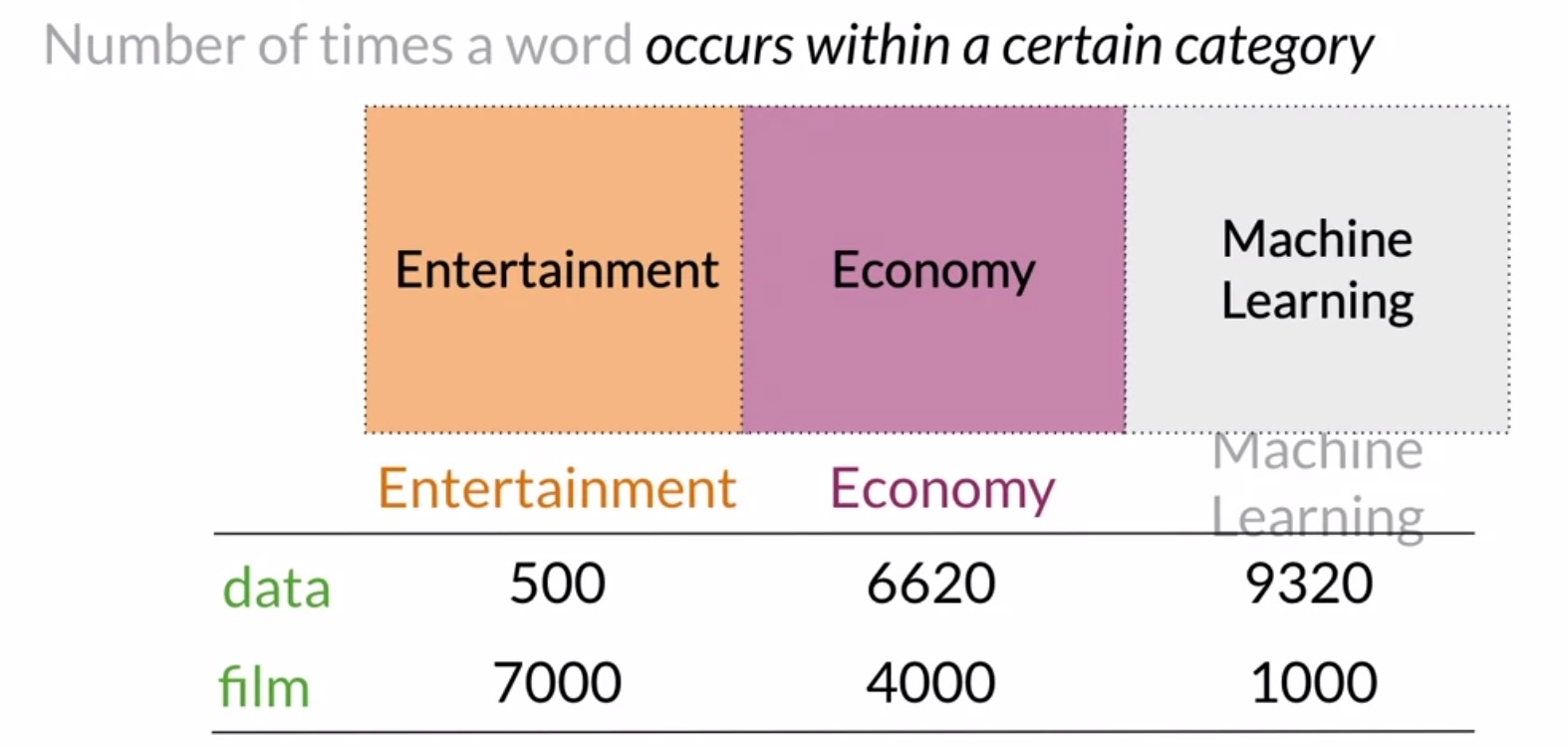
- For instance, you could have a corpus consisting of documents between different topics like entertainment, economy, and machine learning. Next, you would have to count the number of times the word appears in documents that belong to each of the three categories.
In our particular e.g., suppose that the word data appears \(500\) times in documents from your corpus related to entertainment, \(6620\) times in economy documents, and \(9320\) in documents related to machine learning. Similarly, the word film appears in each document’s category \(7000, 4000\) and \(1000\) times respectively.

Once you’ve constructed the representations for multiple sets of documents or words, the next step is to port these to vector space.
Using the matrix we generated, we’ll take the representation for every category of document by looking at the columns. So the vector space will have 2 dimensions – the number of times that the words data and film appear on the type of document.
For the entertainment, economy and machine learning category, you would have the vector representation shown in the below figure. Note that in the vector space, it is easy to see that the economy and machine learning documents are much more similar than they are to the entertainment category.

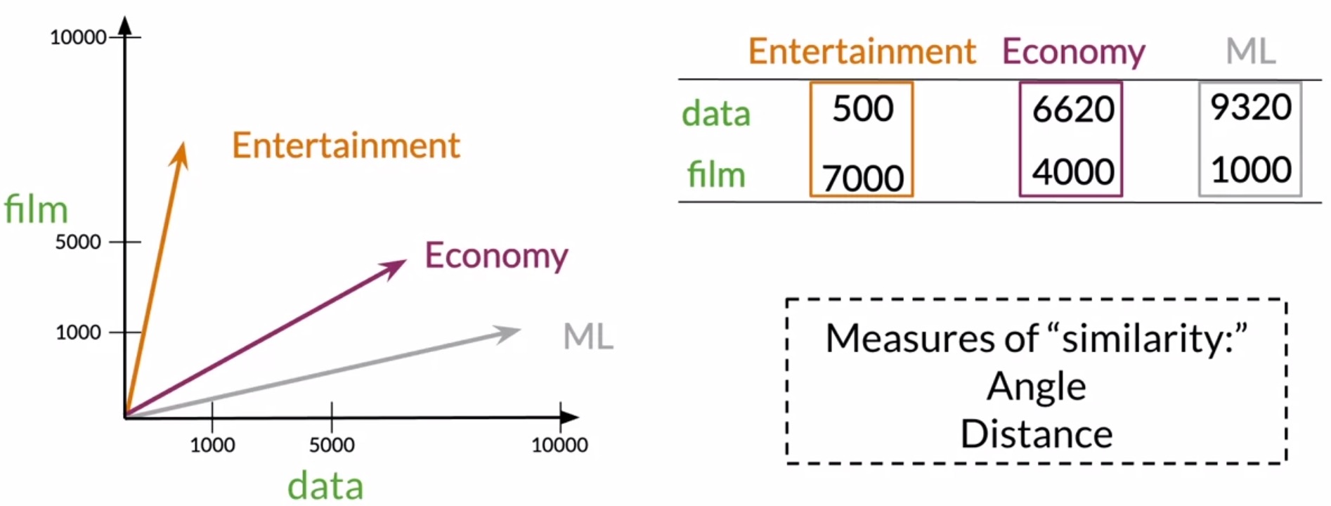
In the next section on Euclidean distance, we’ll look into how we can perform comparisons between vector representations using cosine similarity and the Euclidean distance in order to get the angle and distance between them.
Key takeaways
- You can get vector spaces using two different designs: word by word and word by document.
  - Word by Word: count the co-occurrence of words, i.e., the number of times two words occur together within a certain distance \(k\).
  - Word by Document: count the number of times a word occurs within each category of documents.
- In vector spaces, you can determine the “closeness” or relationships between different types of documents using similarity.

Euclidean distance

In vector space, you can find relationships between words and vectors, such as a measure of their similarity.
Euclidean distance is a similarity metric that allows you to compare two vectors. This metric allows you to identify how far two points or two vectors are apart from each other.
Let’s use 2 of the corpora vectors we saw in the previous section on word by document design. Recall that in that example, there were two dimensions: the number of times that the word data and the word film appeared in the corpus. In the figure below, corpus A is be the entertainment corpus and corpus B is the machine learning corpus.

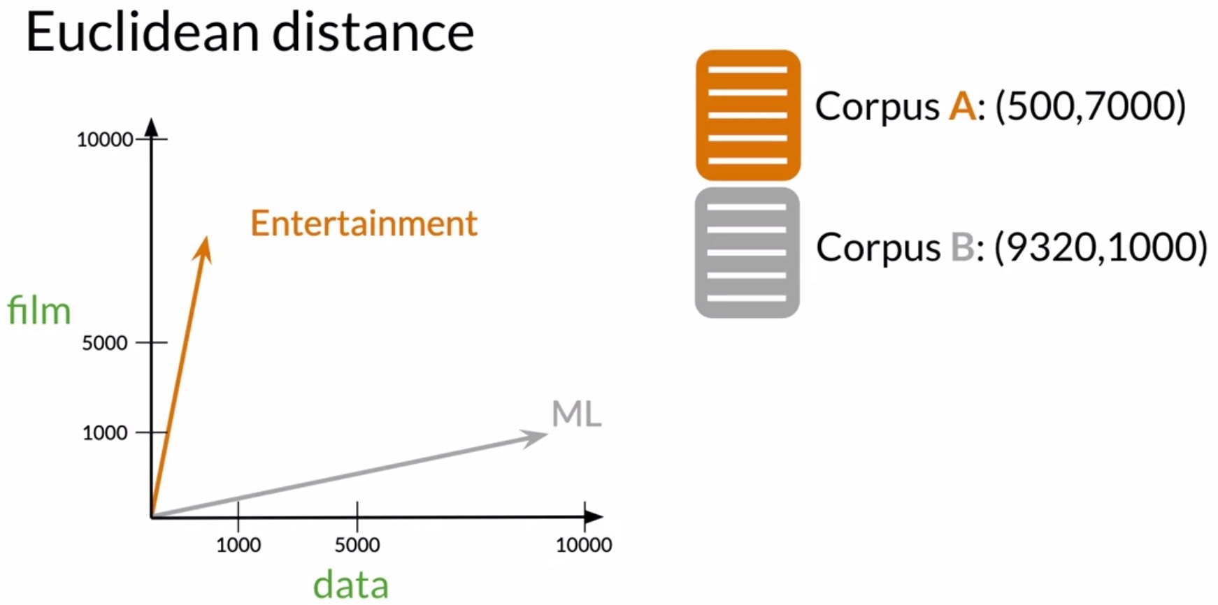
Now let’s represent those vectors as points in the vector space.
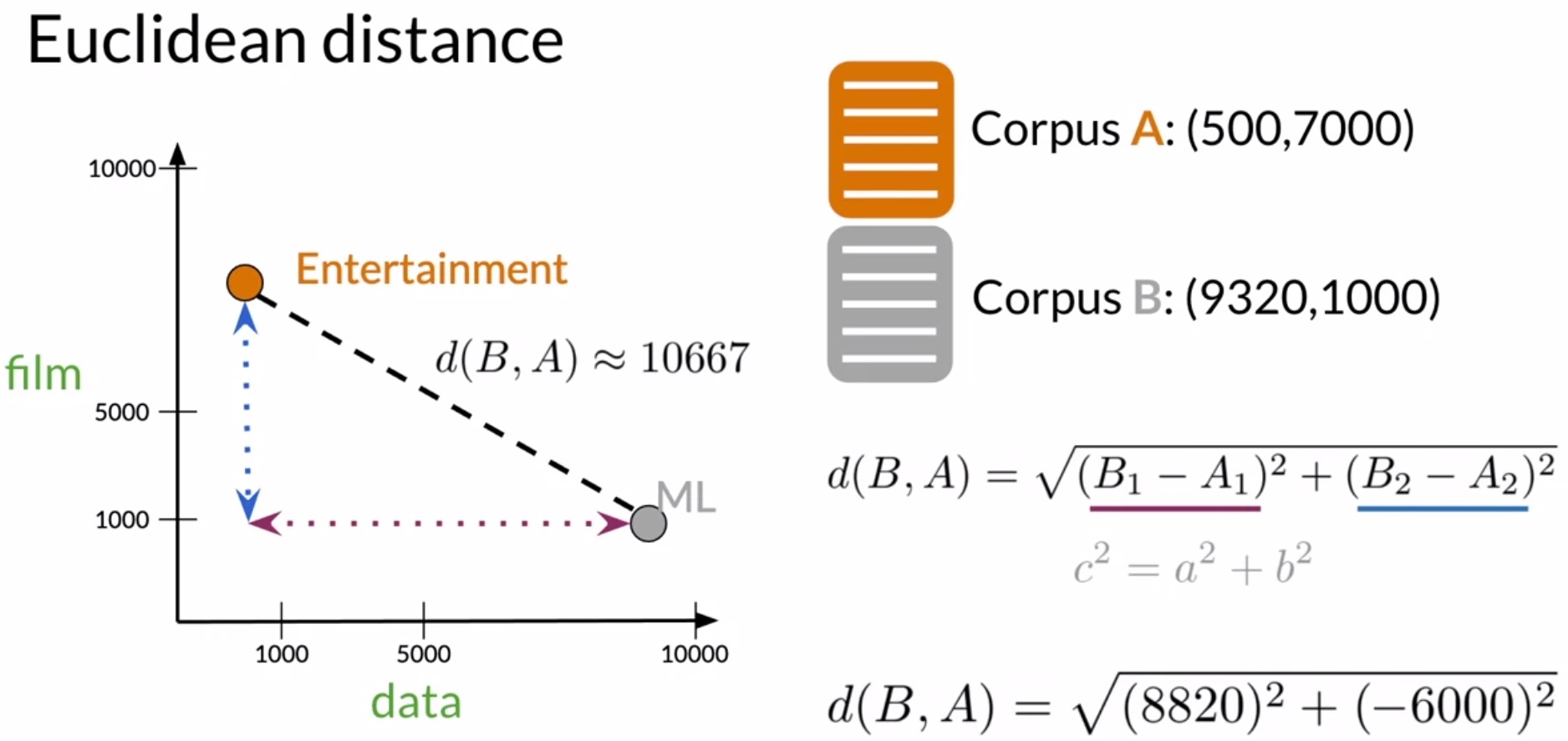
The Euclidean distance is the length of the straight line segment connecting the two points. To obtain the Euclidean distance between two points \(P_1\) and \(P_2\) having co-ordinates \((x_1, y_1)\) and \((x_2, y_2)\), the formula is as follows:

\[d(P_1, P_2) = \sqrt{({x_2} - {x_1})^2 + ({y_2} - {y_1})^2}\]

The first term is the horizontal distance squared and the second term is the vertical distance squared.
Looking deeper, we can observe that this formula follows from the Pythagorean theorem, as shown in the figure below. Using the values in the figure below in the equation to find the distance between corpora \(A\) and \(B\), you will arrive at the expression \(\sqrt{(8820)^2 + (-6000)^2} = 10667\).

Now, let’s generalize the intuition we’ve developed to vector spaces in higher dimensions.
The Euclidean distance extends well to higher dimensions. To get the Euclidean distance between two n-dimensional vectors:
- Get the difference between each of their dimensions.
- Square those differences.
- Sum them up.
- Get the square root of your results.
This process is simply the generalization of the one we saw earlier with 2 dimensions.
Formally, the Euclidean distance between vector representations is given by the following formula:
\[d(v, w) = d(w, v) = \sqrt{({v_1} - {w_1})^2 + ({v_2} - {w_1})^2 + \ldots + ({v_n} - {w_n})^2}\\ = \sqrt{\sum\limits_{i=1}^n{({v_i} - {w_i})^2}}\]
- where,
  - \(v\) and \(w\) are the word vectors whose distance is being calculated.
  - \(n\) is the number of elements in the vector (referred to as an \(n\)-dimensional vector space).
The more similar the words, the more likely the Euclidean distance will be close to 0.
Recall that in linear algebra, this formula is known as the norm of the difference between the points/vectors that you are comparing.
Let’s walk through an example using the co-occurrence matrix shown in the figure below.

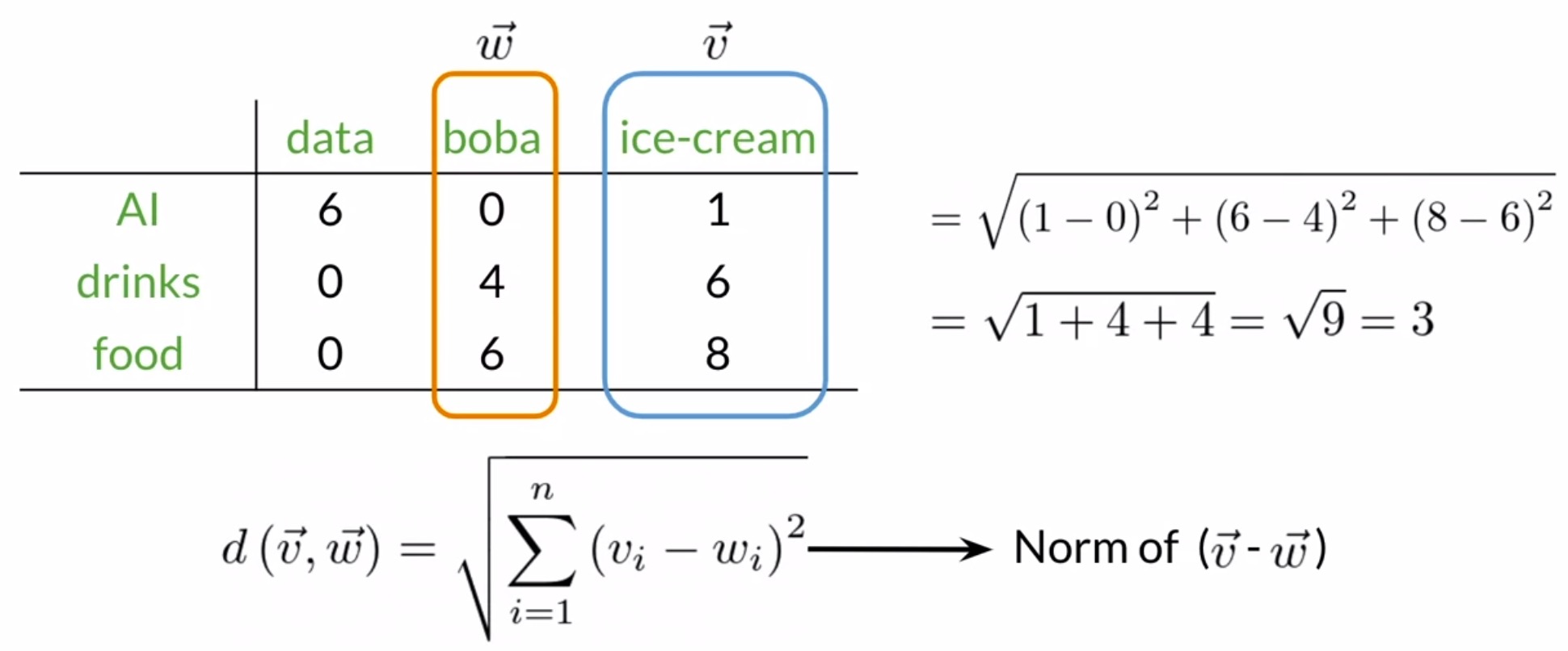
Assuming \(v\) and \(w\) to be the vector representations of the words ice cream and boba, the Euclidean distance between the two vectors is:

\[d(v, w) = \sqrt{(1 - 0)^2 + (6 - 4)^2 + (8 - 6)^2} = \sqrt{1 + 4 + 4} = \sqrt{9} = 3\]

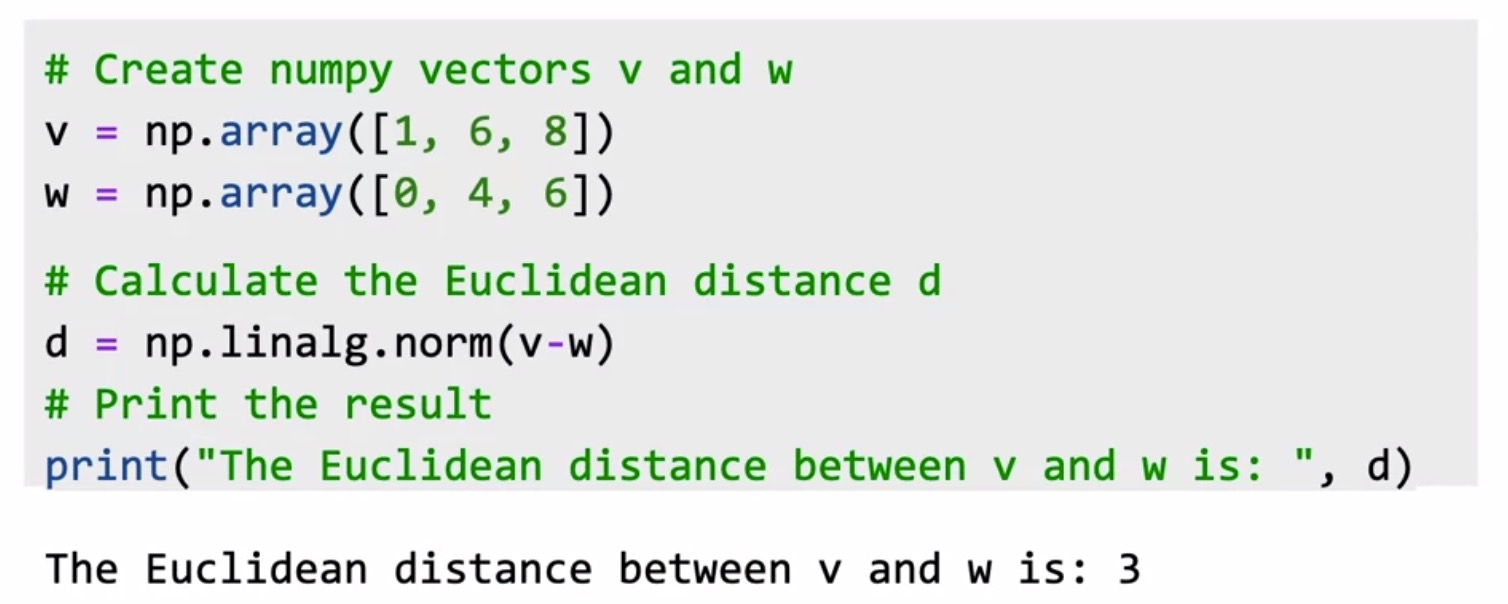
Let’s take a look at the implementation of the Euclidean distance in Python. We can use the linalg module from numpy np.linalg.norm(a-b) to get the norm of the difference between two vectors \(a\) and \(b\). Note that the norm function works for n-dimensional spaces.

Key takeaways
- Euclidean distance is the length of the straight line that connects any two points, i.e., two vectors in vector space.
- To get the Euclidean distance, calculate the norm of the difference between the vectors being compared. By using this metric, you can get a sense of how similar two documents or words are.
- Euclidean distance can however be misleading when the corpora have different sizes.

Cosine similarity

Intuition

The cosine similarity is another similarity function. Using the cosine of the inner angle between the two vectors, it tells you whether two vectors are similar or not.
When comparing vector representations of corpora of different sizes, Euclidean distance can misrepresent the measure of similarity between two vectors. The cosine similarity metric can help overcome this problem.
To illustrate a scenario where the euclidean distance can prove to be problematic, let’s consider the following example.
Suppose that you are in a vector space where the corpora are represented by the occurrence of the words disease and eggs. Shown below in the figure is a representation of the food, agriculture and history corpus. Each one of these corpora have text related to that subject.
However, the corpora differ in the sense that their word totals have a significant mismatch. Specifically, the agriculture and the history corpus have a similar number of words, while the food corpus has a relatively small number.

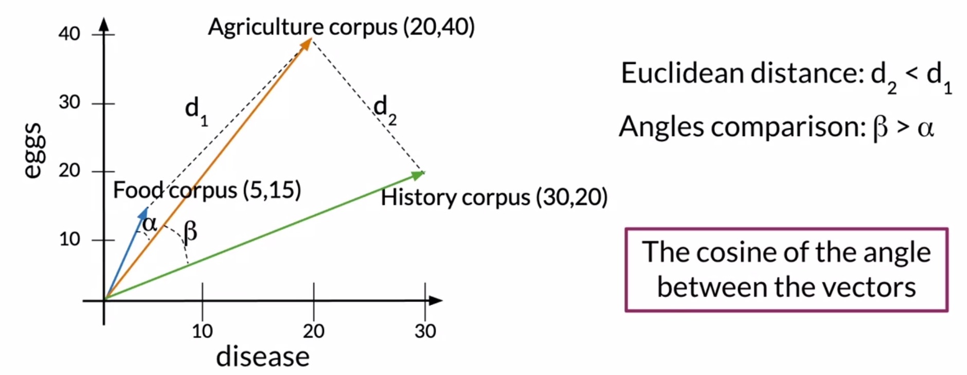
Let’s define the euclidean distance between the food and the agriculture corpus as \(d_1\) and that between the agriculture and the history corpus be \(d_2\).
As you can see, the distance \(d_2\) is smaller than the distance \(d_1\), which suggests that the agriculture and history corpora are more similar than the agriculture and food corpora, which intuitively doesn’t make sense.
Enter cosine similarly, which is a common method for determining the similarity between vectors by computing the cosine of their inner angle.
- If the angle is small, the cosine tends to 1. As the angle approaches \(90^{\circ}\), the cosine tends to 0. This implies that larger the angular delta between the two vectors, lesser the similarity.
- In our particular example shown in the figure above, the angle \(\alpha\) between food and agriculture is smaller than the angle \(\beta\) between agriculture and history, indicating that food and agriculture are more similar than agriculture and history, which gels well with intuition.
Thus, in this case, the cosine of those angles is a better proxy of similarity between these vector representations than their euclidean distance.

Background

Norm of a vector

Recall from linear algebra that the norm (or magnitude) of an n-dimensional vector \(v\) is the square root of the sum of its elements squared:

\[norm(\vec{v})=||\vec{v}||=\sqrt{\sum_{i=1}^{n} v_{i}^{2}}\]

Dot-product of two vectors

The dot product (or scalar product or inner product) between two n-dimensional vectors \(v\) and \(w\) is the sum of the products between their elements in each dimension of the vector space:
\[\vec{v} \cdot \vec{w}=\sum_{i=1}^{n} v_{i} \cdot w_{i}\]
- Note that the two vectors need to be of the same size for their dot product to be defined.
- Also, note that the dot product of two vectors yields a scalar, i.e., a single number.
Finally, note that the norm of a vector can be written as the square root of the dot product of the vector with itself, as shown below:

\[norm(\vec{v})=||\vec{v}||=\sqrt{\sum_{i=1}^{n} v_{i}^{2}}=\sqrt{v \cdot v}\]

For a detailed discussion on the geometric interpretation of the dot product and different ways of calculating it, refer “Engineering Math - Quick Reference: Inner Product/Dot Product”.

Implementation

Let’s explore how we may calculate the cosine similarity metric using the cosine of the inner angle of two vectors.
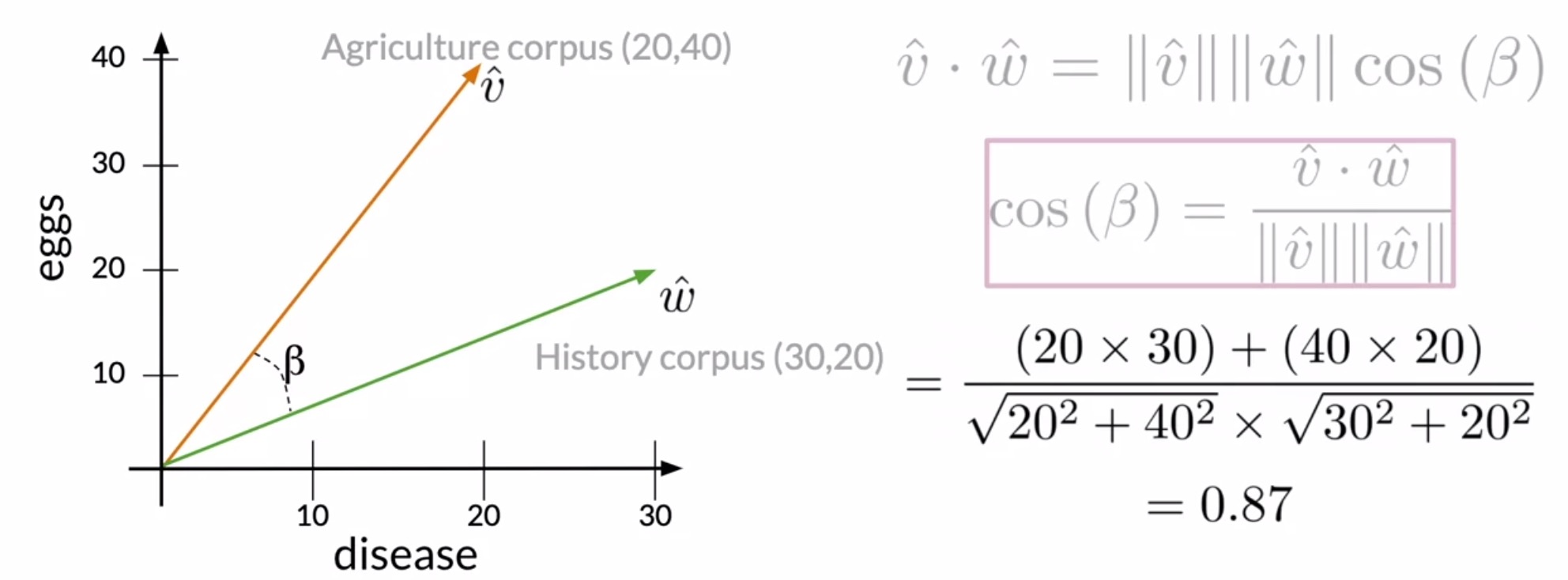
Using the example we discussed in the section on intuition, let’s delve into the similarity of the agriculture and history corpora. Recall that in this example, you have a vector space where the representation of the corpora is given by the number of occurrences of the words disease and eggs.
The angle between those vector representations is denoted by \(\beta\). The agriculture corpus and the history corpus is represented by the vector \(v\) and \(w\) respectively. The dot products between vectors \(v\) and \(w\) is defined as follows:
\[\hat{v} \cdot \hat{w} = ||\hat{v}|| \cdot ||\hat{w}|| \cdot cos(\beta)\\ \Rightarrow cos(\beta) = \frac{\hat{v} \cdot \hat{w}}{||\hat{v}|| \cdot ||\hat{w}||}\\ \therefore cos(\beta) = \frac{\sum_{i=1}^{n} v_{i} w_{i}}{\sqrt{\sum_{i=1}^{n} v_{i}^{2}} \sqrt{\sum_{i=1}^{n} w_{i}^{2}}}\]
- where \(v\) and \(w\) represent the word vectors and \(v_{i}\) or \(w_{i}\) represent index \(i\) of the respective vector.
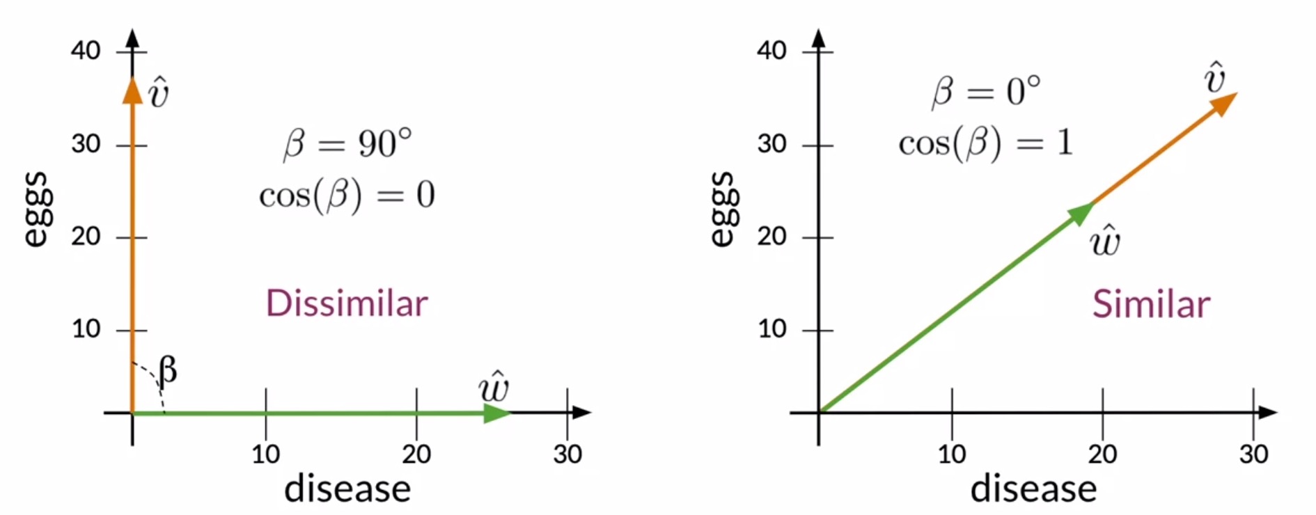
Interpreting the output of cosine similarity depending on the angle between vectors \(v\) and \(w\):
- If the vectors are identical, you get \(cos(\theta) = cos(0) = 1\).
- If the vectors are opposites, i.e., \(A = −B\), you get \(cos(\theta) = cos(180^\circ) = -1\).
- If the vectors are orthogonal (or perpendicular), you get \(cos(\theta) = cos(90^\circ) = 0\).
Also, interpreting the output of cosine similarity depending on the magnitude of the output:
- An output \(\in [0, 1]\) indicates a similarity score.
- An output \(\in [-1, 0]\) indicates a dissimilarity score.
Thus, the cosine of the inner angle \(\beta\) between the two vectors is given by the dot product between the vectors \(v\) and \(w\) divided by the product of the two norms.
Replacing the actual values from the vector representations should give you this expression in the figure below.
- In the numerator, you have the product between the occurrences of the words, disease and eggs.
- In the denominator, you have the product between the norm of the vector representations of the agriculture and history corpora.
- Ultimately, you obtain a cosine similarity of \(0.87\).

Next, let’s delve into how the value of the cosine similarity is related to the similarity of two vectors, as shown in the figure below.
- Consider the case where two vectors are orthogonal in a vector space. Note that it is only possible to have positive values for any dimension, which implies that the maximum angle between pair of vectors is \(90^{\circ}\). In this case, the cosine would be equal to 0, and it would mean that the two vectors have orthogonal directions or that they are maximally dissimilar.
- Now, let’s look at the case where the vectors have the same direction. In this case, the angle between them is \(0^{\circ}\) and the cosine is equal to 1, because the cosine of 0 is 1.
- Thus, as the cosine of the angle between two vectors approaches 1, the closer their directions are.

Cosine similarity outputs values \(\in [0, 1]\).
To calculate the cosine similarity between vectors \(a\) and \(b\) using numpy:

import numpy as np

# Create numpy vectors v and w
a = np.array([1, 0, -1, 6, 8])
b = np.array([0, 11, 4, 7, 6])

cosine_similarity = np.dot(a, b) / (np.linalg.norm(a) * np.linalg.norm(b))

Key takeaways
- The cosine similarity between a pair of vectors is proportional to the similarity between the directions of the vectors that you are comparing.
- (+) The intuition behind the use of the cosine similarity as a metric to compare the similarity between two vector representations is that it isn’t biased by the size difference between the representations. This is the main advantage of the cosine similarity metric over euclidean distance.
- For two vectors \(v, w\) the cosine of their inner angle \(\beta\) is given by:
```
  np.dot(a, b) / (np.linalg.norm(a) * np.linalg.norm(b)
```
- Cosine similarity outputs values \(\in [0, 1]\). On the other hand, an output \(\in [-1, 0]\) indicates the degree of dissimilarity.

Word manipulation in vector spaces

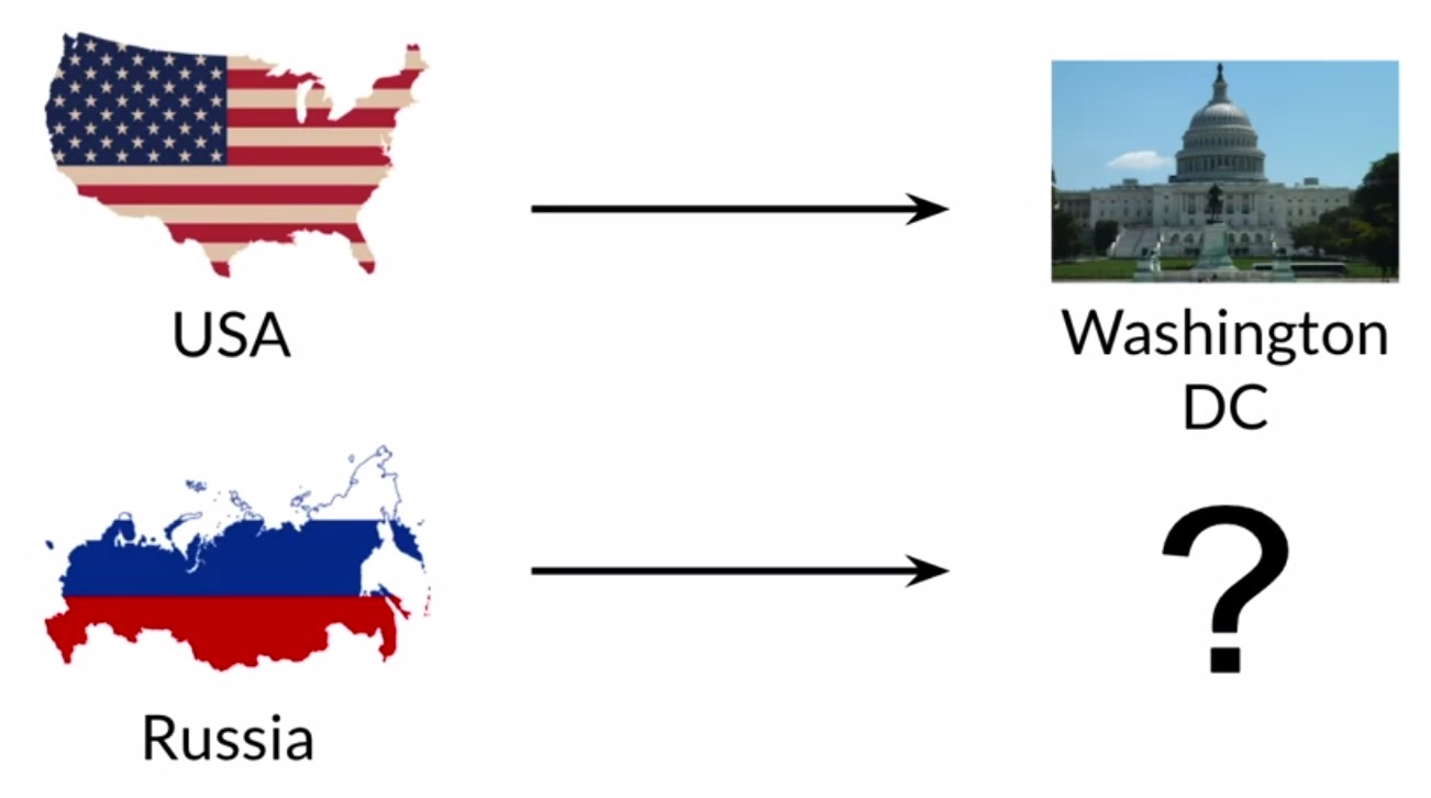
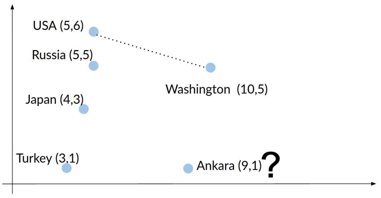
Let’s perform vector manipulation using simple vector arithmetic, i.e., by adding vectors and subtracting vectors. We’ll apply the idea of manipulate vector representations to the task of inferring unknown relationships among words, such as predicting the countries of certain capitals.
Suppose that you have a vector space with countries and their capital cities. While you know that the capital of the United States is Washington DC, you don’t know the capital of Russia, but you would like to use the known relationship between Washington DC and the USA to figure it out. Vector manipulation involves using some simple vector algebra to carry out such tasks.

For this particular example, let’s assume that you are in a hypothetical two-dimensional vector space that has different representations for different countries and capitals cities.
First, you will have to find the relationship between the Washington DC and USA vector representations. In other words, we need to figure out the vector that connects Washington DC and USA. To do so, get the difference between the two vectors. This vector will tell you how many units on each dimension you’ll need to move in order to find a country’s capital in that vector space.
To find the capital city of Russia, all you have to do is to sum it’s vector presentation with the difference vector.
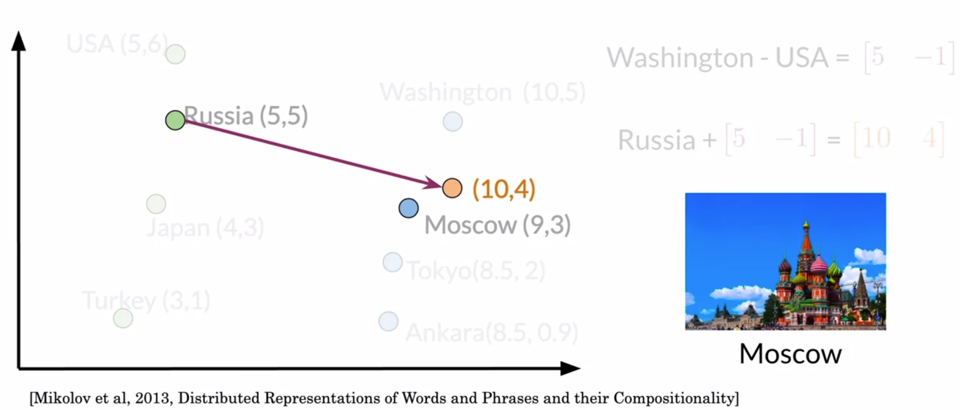
You thus deduce that the capital of Russia has a vector representation of \((10, 4)\).

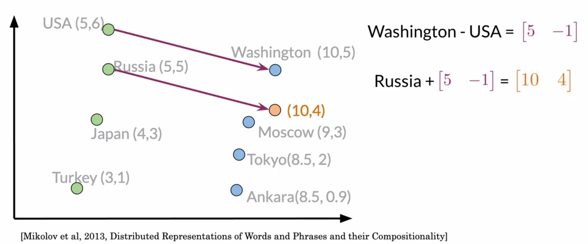
However, since here are no cities with that representation, you’ll have to take the one that is the closest to it by comparing each vector with the Euclidean distances or cosine similarities. In this case, the vector representation that is closest to \((10, 4)\) is the one for Moscow.
Thus, using this simple process, we could predict the capital of Russia knowing the capital of the USA. The only requirement here is that you need a vector space where the representations capture the relative meaning of words.

Let’s take another example. Using the same method, let’s predict the country whose capital is Ankara. Turkey is the answer with an Euclidean distance \(d\) between your prediction vector and the correct vector as \(1.41\).

Key takeaways
- (+) Vector manipulations enable deriving unknown relationships between words using known relationships. This speaks to the importance of vectors spaces where the representations of words capture the relative meaning in natural language.
- With the above vector representations, we’ve explored the clustering of all vectors when plotted in a 2D setting, where the vectors of the words have similar contexts are encoded similarly.
- This type of encoding consistency lends itself to identifying patterns.
  - For e.g., to find the closest words to the word doctor by computing cosine similarity, you’ll come across nurse, cardiologist, surgeon, etc.

PCA

Visualization of word vectors

Often, you’ll end up having vectors in very high dimensions. While operating on such vectors in very high dimensional spaces might be computationally feasible, it is impossible to visualize results in such high dimensional spaces. To visualize word vectors on an XY plane in order to identify relationships between words, we’ll need a way to reduce its dimension-space to 2 dimensions.
Principal Component Analysis (PCA) allows you to do so. PCA enables visualization of vector representations with high dimensions by projecting them onto a lower-dimensional space.
Let’s begin by motivating the idea of visualizing vector presentation of words. Shown below is an example of vector representation for some words in a vector space.

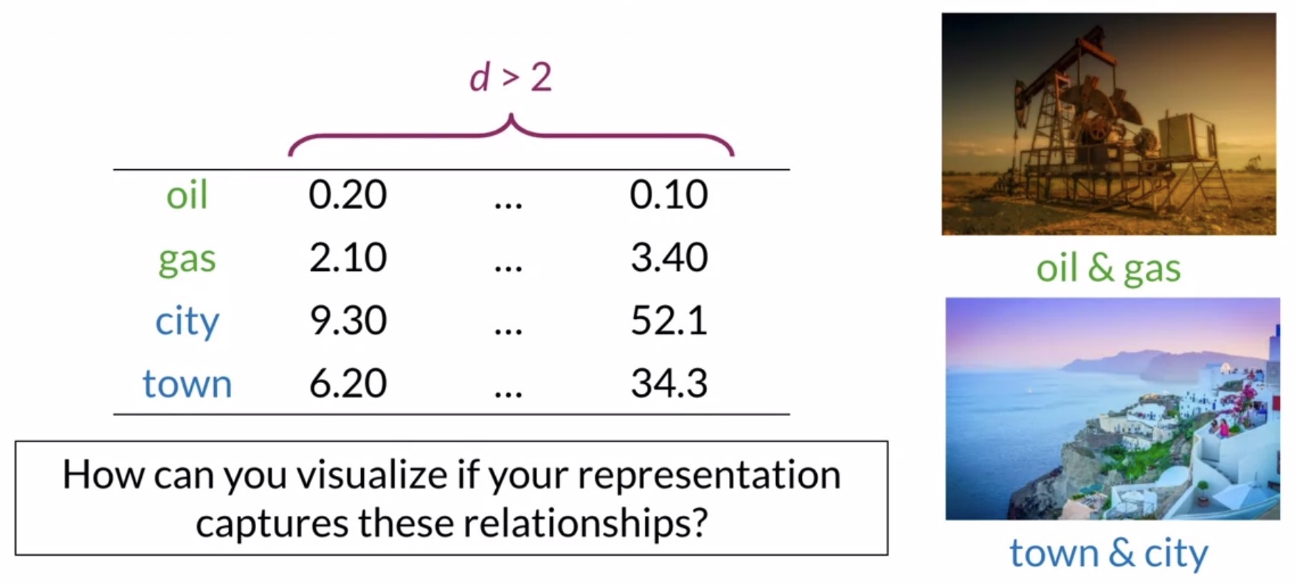
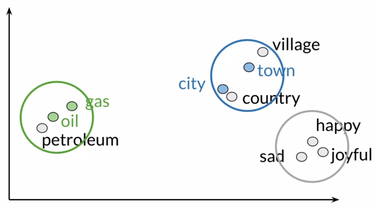
To represent a set of words in the 2D space that currently exist in a high dimensional space, dimensionality reduction is of essence. PCA enables you to get a representation in a vector space with fewer dimensions. To ease the process of visualization of data, you can get a reduced representation with fewer features (say, 2 or 3).

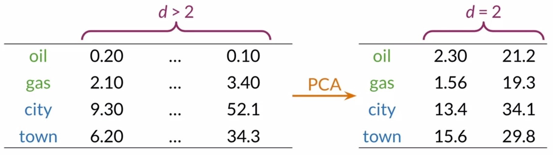
Applying PCA on your data can get you a 2D representation, which you can then use to plot an XY visual of your words. In our particular example, you might find that your initial representation captured the relationship between the words oil, gas, city and town since they appear to be clustered with related words in your two-dimensional space. You can even find other relationships among your words that you didn’t expect, which is a fun and useful possibility!

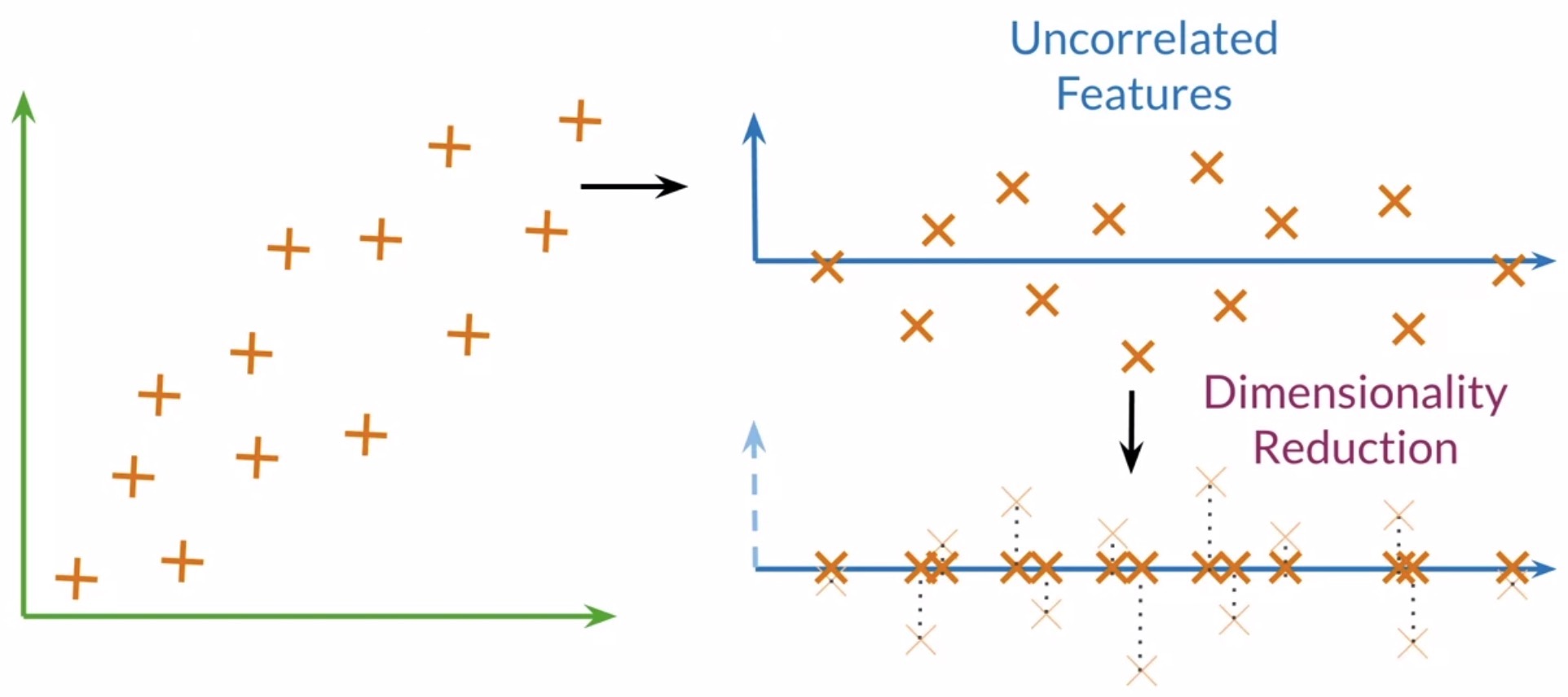
Let’s look into a quick overview on how PCA works. We’ll begin with a 2D vector space for the sake of simplicity. Say that you want your data to be represented by one feature instead.
- Using PCA, you’ll find a set of uncorrelated features.
- These uncorrelated features are then projected to a one dimensional space, while trying to retain as much information as possible. In this case, by retaining maximum information we mean that the Euclidean distance between the original vectors and their projected siblings is minimal. Hence, vectors that were originally close in the embeddings dictionary will produce lower dimensional vectors that are still close to each other.

Key takeaways
- PCA is an algorithm used for dimensionality reduction that can find uncorrelated features in your data. It’s helpful for visualizing your data to check if your representation is capturing relationships among words.
- After obtaining uncorrelated features, PCA projects your data representation to a lower dimension while retaining as much information as possible.

Implementation

Let’s learn about the underlying concepts behind PCA, namely eigenvectors and eigenvalues from the covariance matrix of your data, and how they help to carry out dimensionality reduction of your features.
Recall the concepts of eigenvectors and eigenvalues of matrices from algebra. While the exact implementation details behind eigenvectors and eigenvalues are irrelevant for the purposes of our discussion, the point to note is that PCA utilizes these concepts under-the-hood. Once the covariance matrix is obtained from the original data, the eigenvectors yield directions of uncorrelated features, while the eigenvalues represent the variance of your data on each of those new features.
Now let’s delve into the implementation process.
Get uncorrelated features
- To get a set of uncorrelated features, you will need to normalize your data, get the covariance matrix, and finally, perform Singular Value Decomposition (SVD) on the covariance matrix to get a set of 3 matrices. Note that SVD is already implemented in popular numerical libraries such as NumPy so we can abstract away its implementation details for now.
- The first of those matrices contains the eigenvectors stacked as column vectors. The second one has the eigenvalues on the diagonal, as shown graphically below:

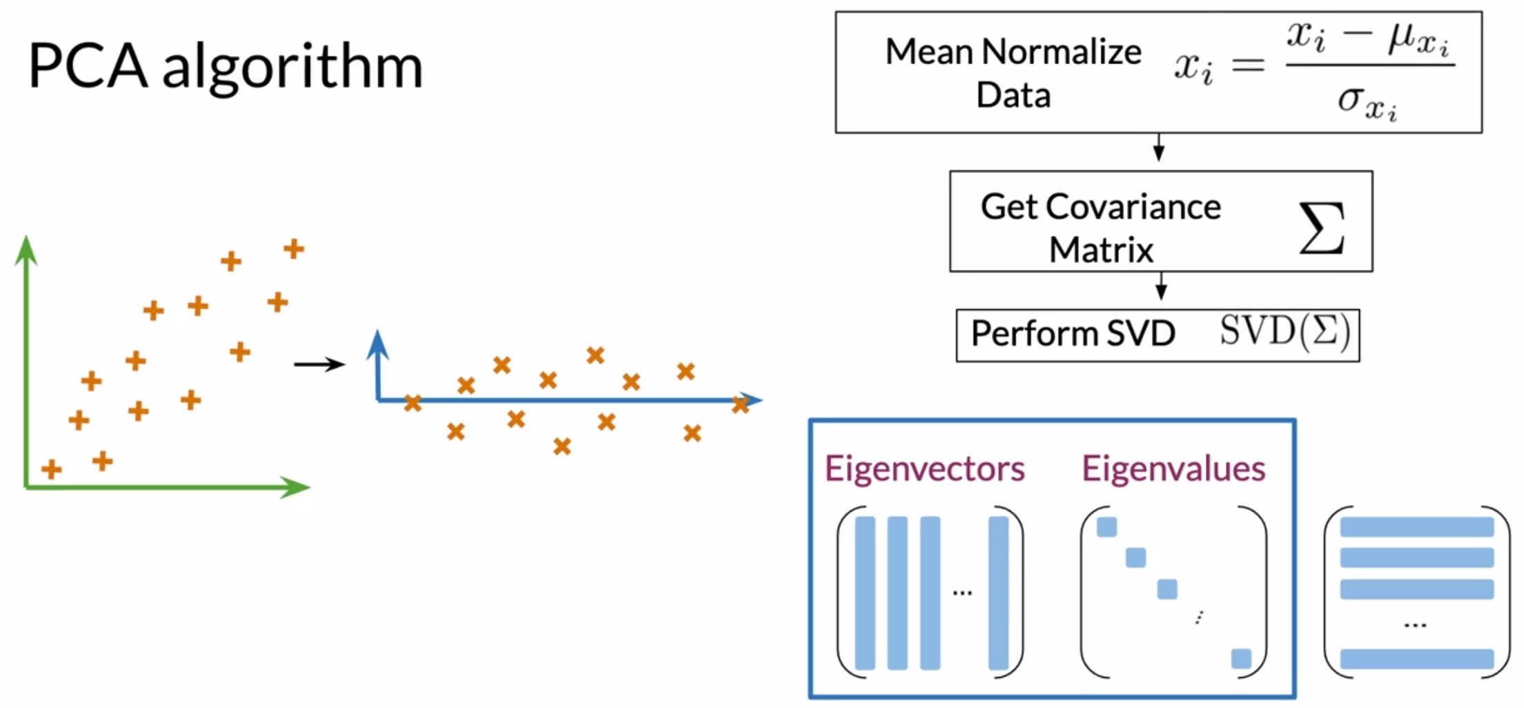
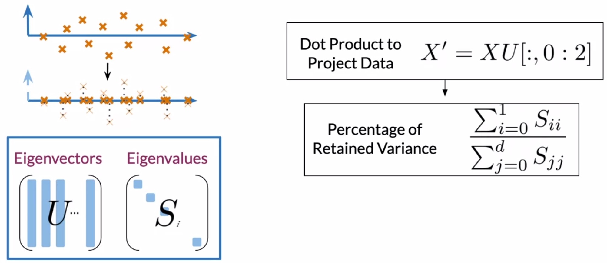
Project uncorrelated features to a lower-dimensional vector space
- The next step is to project your data to a new set of features. This step involves using the eigenvectors and eigenvalues obtained in the previous step.
- Let’s denote the eigenvectors with \(U\) and the eigenvalues with \(S\).
1. Dot-products between your data and eigenvectors: perform dot products between the matrix containing your word embeddings and the first \(n\) columns of the \(U\) matrix, where \(n\) denotes the desired number of dimensions. For visualization, it is common practice to have 2 or 3 dimensions.
2. Variance in the new vector space: Using the eigenvalues, you’ll get the percentage of variance retained in the new vector space.
As an important side note, for the purposes of dimensionality reduction, the principal components contained in the rotation matrix, i.e., the eigenvectors, should be sorted in descending order of the explained variance, i.e., the eigenvalues. In other words, the features with the highest variance should appear first.
- This implies that the first components retain most of the power to explain the patterns that generalize the data.
- This also ensures that you retain as much information as possible from your original embedding.
- Nevertheless, for other opposing applications such as novelty detection, we are usually interested in the patterns that explain much less variance, in which case the principal components are usually sorted in the ascending order of the explained variance.
- Note that most numerical libraries sort these matrices for you.

t-SNE is another visualization method, that is particularly well suited for the visualization of high-dimensional datasets. It is extensively applied in image processing, NLP, genomic data and speech processing. Read more on it in CS231n | Visualizing and Understanding.
Key takeaways
- Goals
  - (+) PCA enables high-dimensional data visualization by carrying out dimensionality reduction to represent data in a reduced space of uncorrelated variables, say on a 2D plane.
- Process
  - At a top level, PCA involves the following steps:
    - Get uncorrelated features: Using the word representations in your original vector space, get uncorrelated features.
    - Project uncorrelated features to a lower-dimensional vector space: Reduce the dimensionality of your data by projecting your data to a vector space with the desired number of features, while trying to retain as much information as possible from your original embedding.
- Concepts
  - PCA is based on the Singular Value Decomposition (SVD) of the covariance matrix of the original high dimensional dataset.
  - Eigenvectors from the “decomposed” covariance matrix contain the principal components, which are encoded as a rotation matrix that contains the directions of the uncorrelated features.
  - Eigenvalues associated with the aforementioned eigenvectors represent the “explained variance” of each principal component, i.e., variance of your data on the new features. In other words, they signal the amount of information retained by each new feature.
- Implementation
  - Get uncorrelated features
    1. Mean normalize data by operating on each feature separately (across the entire dataset).
    2. Compute the covariance matrix.
    3. Perform SVD on the covariance matrix to get the eigenvectors and eigenvalues.
  - Project uncorrelated features to a lower-dimensional vector space
    1. The dot product of your word embeddings and the eigenvectors matrix will project your data onto a new vector space of the desired dimension.
    2. Compute the amount of retained variance (in %) using the eigenvalues.

Putting it together with code

Let’s string together our learnings into a program performs PCA on a dataset where each row corresponds to a word vector in a high dimensional space (say, \(300\)). This implies that the dimensions of the dataset would be \((m, n)\), where \(m\) are the number of observations, i.e., the words in the dataset and \(n = 300\) are the number of features/dimensions per observation/word.
The goal is to use PCA to transform \(300 \rightarrow n\_components\) dimensions.
The shape of the “reduced” matrix should be \((m, n\_components)\).
Here are the steps involved in performing PCA on our dataset:

Mean normalize (also referred to as de-meaning the data).
- Use np.mean(a,axis=None). Recall that each row is a word vector, and the number of columns are the number of dimensions in a word vector.
- If you set axis = 0, you take the mean for each column. If you set axis = 1, you take the mean for each row.
Get the covariance matirx.
- Use np.cov(m, rowvar=True). This calculates the covariance matrix. By default, rowvar is True.
  - From the NumPy documentation: “If rowvar is True (default), then each row represents a variable, with observations in the columns.”
- Note that in our case, each row is indeed a vector observation for a particular word, and each column is a feature for that word, which is why rowvar is set to True.
Get the eigenvalues using np.linalg.eigh(). Use eigh rather than eig since R is symmetric. The performance gain when using eigh instead of eig is substantial.
- Use np.linalg.eigh(a, UPLO='L').
Sort the eigenvectors and eigenvalues by decreasing order of the eigenvalues.
- Use np.argsort() to sort the values in an array from smallest to largest, then returns the indices from this sort.
- In order to reverse the order of a list, you can use: x[::-1].
Get a subset of the eigenvectors (choose how many principal components you want to use using n_components).
- To apply the sorted indices to eigenvalues, you can use x[indices_sorted].
- When applying the sorted indices to eigenvectors, note that each column represents an eigenvector. In order to preserve the rows but sort on the columns, you can use x[:, indices_sorted].
Return the transformed dataset by multiplying the eigenvectors with the original data.
- To transform the data using a subset of the most relevant principal components, take the matrix multiplication of the eigenvectors with the original data.
- The shape of the original data is \((m, n)\). The subset of eigenvectors are in a matrix of shape \((n, n\_components)\).
- To multiply these together, take the transposes of both the eigenvectors \((n\_components, n)\) and the data \((n, m)\). The product of these two has dimensions \((n\_components, m)\).
- Finally, take its transpose to obtain \((m, n\_components)\), which is the desired shape.

def compute_pca(X, n_components=2):
    """
    Input:
        X: of dimension (m, n) where each row corresponds to a word vector
        n_components: Number of components you want to keep.
    Output:
        X_reduced: original data transformed into  dims/columns + regenerated 
    """

    # mean center the data
    X_demeaned = X - np.mean(X, axis=0)
    
    # calculate the covariance matrix
    covariance_matrix = np.cov(X_demeaned, rowvar=False)

    # calculate eigenvectors & eigenvalues of the covariance matrix
    eigen_vals, eigen_vecs = np.linalg.eigh(covariance_matrix, UPLO='L')
    
    # sort eigenvalue in increasing order (get the indices from the sort)
    idx_sorted = np.argsort(eigen_vals)
    
    # reverse the order so that it's from highest to lowest.
    idx_sorted_decreasing = idx_sorted[::-1]
    
    # sort the eigenvalues by idx_sorted_decreasing
    eigen_vals_sorted = eigen_vals[idx_sorted_decreasing]

    # sort eigenvectors using the idx_sorted_decreasing indices
    eigen_vecs_sorted = eigen_vecs[:,idx_sorted_decreasing]

    # select the first n eigenvectors (n is desired dimension
    # of rescaled data array, or dims_rescaled_data)
    eigen_vecs_subset = eigen_vecs_sorted[:, 0:n_components]

    # transform the data by multiplying the transpose of the eigenvectors 
    # with the transpose of the de-meaned data
    # Then take the transpose of that product.
    X_reduced = np.dot(eigen_vecs_subset.T, X_demeaned.T).T

    return X_reduced

Document as a vector

To represent a document as a vector, simply add up the word vectors for its constituent words.
Programmatically:

import numpy as np

word_embeddings = {
                    "I":        np.array([1,  0,  1]), 
                    "love":     np.array([-1, 0,  1]),
                    "learning": np.array([1,  0,  1])
                  }
words_in_document = ['I', 'love', 'learning', 'not_a_word']

document_embedding = np.array([0, 0, 0])
for word in words_in_document:
    document_embedding += word_embeddings.get(word, 0)
    
print(document_embedding) # Prints [1 0 3]

Citation

If you found our work useful, please cite it as:

@article{Chadha2020DistilledWordEmbeddingsandVectorSpaces,
  title   = {Word Embeddings and Vector Spaces},
  author  = {Chadha, Aman},
  journal = {Distilled Notes for the Natural Language Processing Specialization on Coursera (offered by deeplearning.ai)},
  year    = {2020},
  note    = {\url{https://aman.ai}}
}

Vector space models

Word by word design

Word by document design

Euclidean distance

Cosine similarity

Intuition

Background

Norm of a vector

Dot-product of two vectors

Implementation

Word manipulation in vector spaces

PCA

Visualization of word vectors

Implementation

Putting it together with code

Document as a vector

Further reading

Citation