Coursera-NLP | Sentiment Analysis using Naive Bayes
- Probability: Basics
- Conditional probability
- Bayes’ rule
- Computing the conditional probabilities table
- Laplacian smoothing
- Naive Bayes
- Further reading
- Citation
Probability: Basics
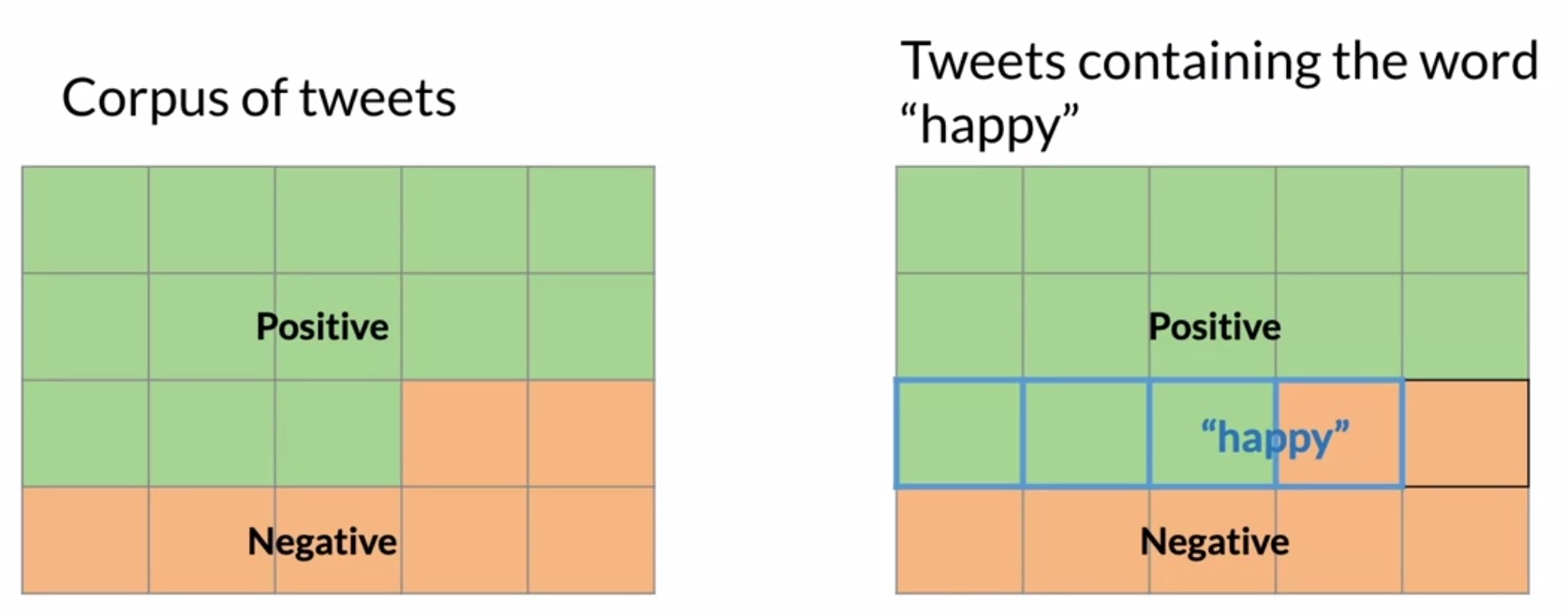
- Imagine you have a corpus of \(20\) tweets that can be categorized as having either positive or negative sentiment, but not both.
- Within that corpus, the word happy is sometimes being labeled positive and in some cases, negative.
- This implies that there exist negative tweets that contain the word happy.
- Conversely, (and obviously) there exist other words apart from happy in tweets labeled positive.
- Shown below is a graphical representation of this “overlap”. Let’s explore how we may handle this case using probability, with a Venn diagram-based graphical interpretation.
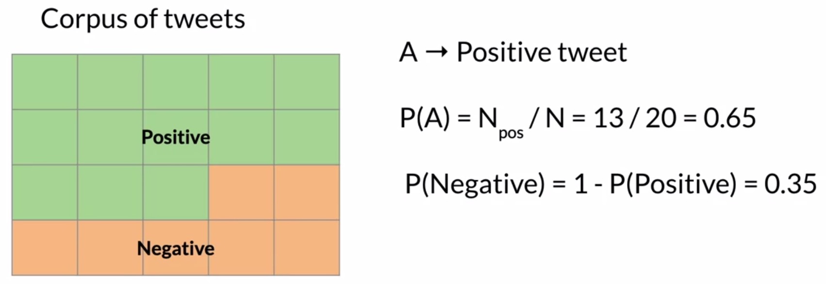
- One way to think about probabilities is by counting how frequently events occur. Let’s define event \(A\) as a tweet being labeled positive. The probability of event \(A\), denoted by \(P(A)\), is calculated as:
- In the example shown in the figure below, \(P(A) = \frac{13}{20} = 0.65\), or \(65\%\). It’s worth noting the complementary probability here, which is:
- Note that for this to be true, all tweets must be categorized as either positive or negative but not both.
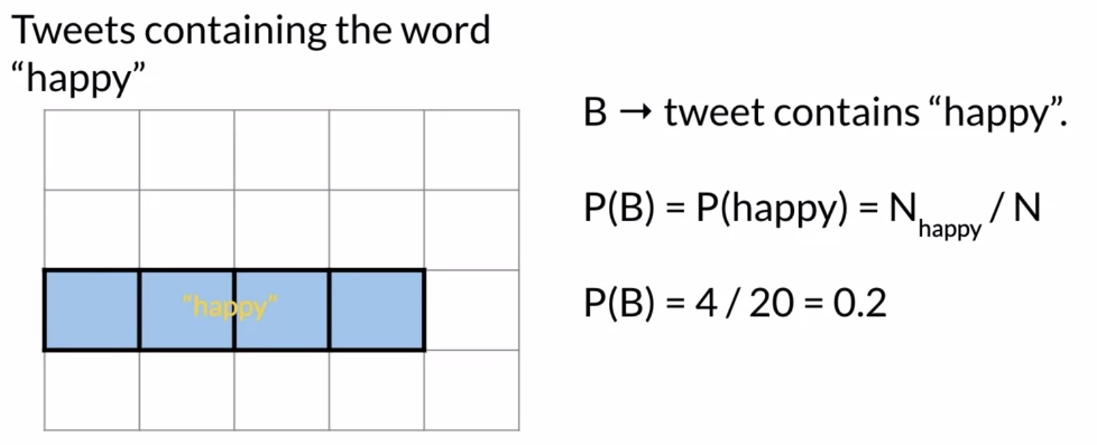
- Next, let’s define event \(B\) in a similar way by counting tweets containing the word happy.
- In the example shown in the figure below, the total number of tweets containing the word happy \(N_{happy}\) is 4. The probability of event \(P(B)\) is thus \(\frac{4}{20} = 0.2\), or \(20\%\).
- From the diagram on the left-hand-side of the figure below, we can infer that there are 3 tweets that are labeled positive and contain the word happy (corresponding to the 3 overlapping cells that are colored pink).
- Another way of looking at this is shown in the Venn diagram in the right-hand-side of the figure below. In particular, notice the intersection of (i) the set of tweets which are labeled positive and, (ii) the set of tweets which contain the word happy.
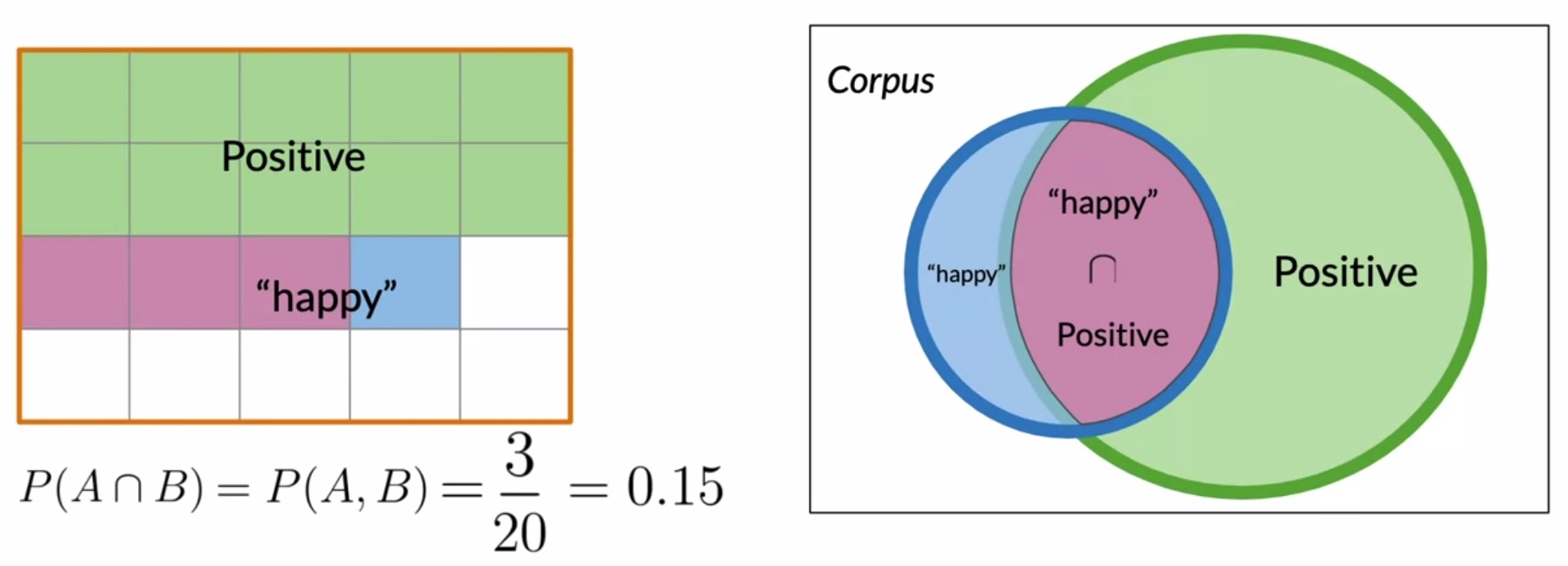
- Recall that the corpus contains \(20\) tweets overall. In the context of the Venn diagram above, the associated probability is:
Conditional probability
- The goal of this section is to derive Bayes’ rule from the concept of conditional probabilities.
- Consider the tweets that contain the word happy, instead of the entire corpus. In other words, from our Venn formulation in the right-hand-side of the diagram below, you would be only considering the tweets inside the blue circle where many of the other positive tweets (that don’t contain the word happy) are now excluded. Note that the purple area in the figure below denotes the probability that a positive tweet contains the word happy.
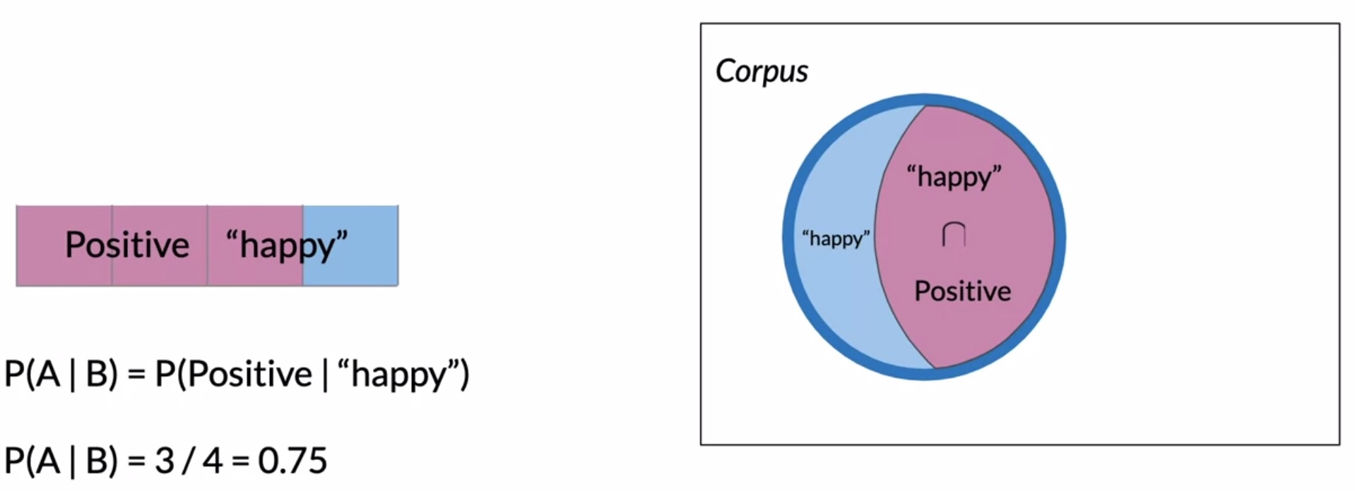
- In this scenario, the probability that a tweet is positive given that it contains the word happy, denoted by \(P(\text{positive | “happy”})\), simply becomes:
- For the particular example in the above figure, \(P(\text{positive | “happy”}) = \frac{3}{4} = 0.75\text{ or 75%}\).
- Thus, a tweet has a 75% likelihood of being positive if it’s contains the word happy.
- Now, keeping the overall Venn diagram from our previous section in mind, think about the inverted case where you’re trying to fiure out the probability of whether a tweet contains the word happy given the tweet is labelled positive. Again, the purple area in the figure below denotes the probability that a positive tweet contains the word happy.
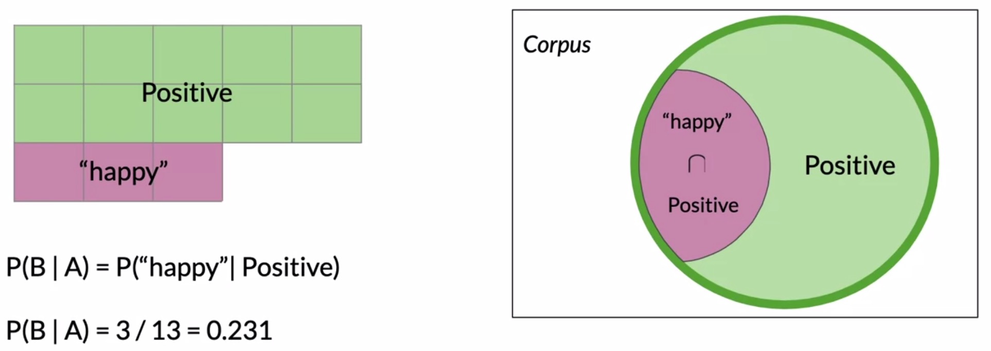
- Formally, the probability \(P(\text{“happy” | positive})\) is:
-
For the particular example in the above figure, \(P(\text{“happy” | positive}) = \frac{3}{13} = 0.23\text{ or 23%}\).
-
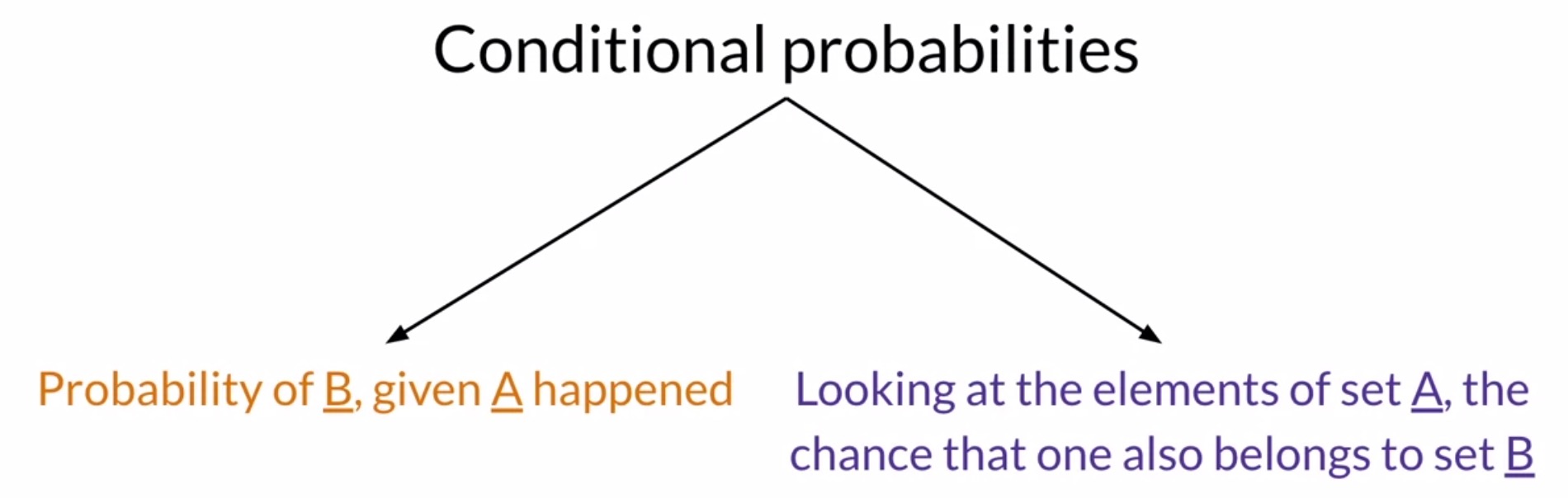
With all of this discussion of the probability of meeting certain conditions, we are essentially talking about conditional probabilities. Conditional probabilities can be interpreted as the probability of an outcome \(B\) knowing that event \(A\) has already happened. In other words, given that we’re looking at an element from set \(A\), the probability that it also belongs to set \(B\).
Bayes’ rule
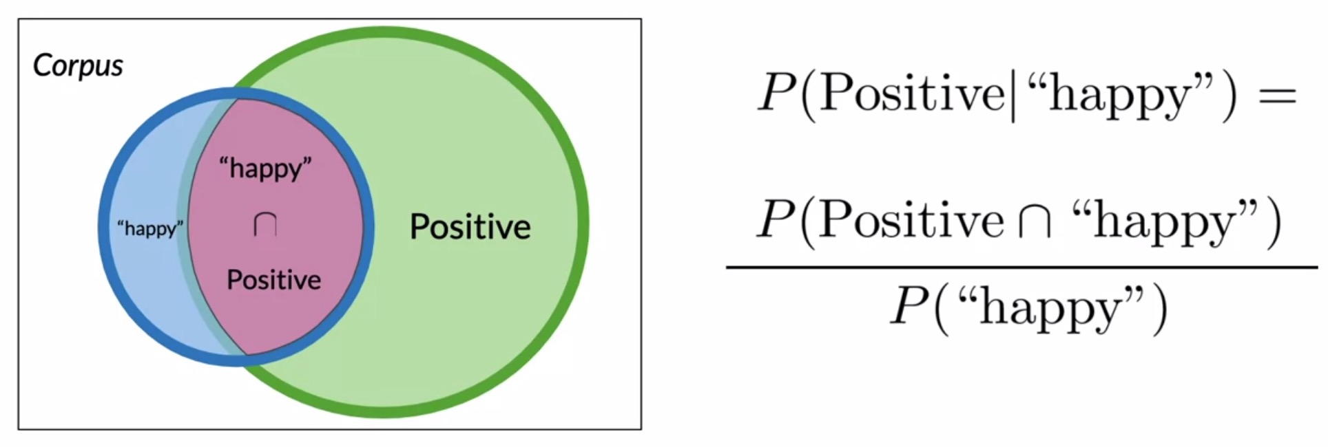
- A graphical way to interpret this is using the the Venn diagram shown below. Using the previous example as reference, the probability of a tweet being positive given that it has the word happy is:
- Let’s take a closer look at the equation from the previous slide. You could write a similar equation by simply swapping the position of the two conditions. This gives you the conditional probability of a tweet containing the word happy given that it is a positive tweet as:
- Armed with both of these equations, you’re now ready to derive Bayes’ rule. To combine these equations, note that the intersections \(\text{“happy” }\cap\text{ positive}\) and \(\text{positive }\cap\text{ “happy”}\) represent the same quantity, no matter which way it’s written.
- Think about the probability of a tweet being positive given that it contains the word happy \(P(\text{positive | “happy”})\) in terms of the probability of a tweet containing the word happy given that it is positive \(P(\text{“happy” | positive})\), with a little algebraic manipulation:
- This is now an expression of Bayes’ rule in the context of our sentiment analysis problem.
- More generally, Bayes’ rule states that:
- This is the basic formulation of Bayes’ rule using expressions of conditional probability. With Bayes’ rule, you can calculate the probability of \(X\) given \(Y\) \(P(X | Y)\) if you already know the probability of \(Y\) given \(X\) \(P(Y | X)\), and the ratio of the probabilities of \(X\) and \(Y\).
- As an example, suppose that in your dataset, \(25\%\) of the positive tweets contain the word ‘happy’, \(13\%\) of the tweets in your dataset contain the word happy, and \(40\%\) of the total number of tweets are positive. You observe the tweet:
'happy to learn NLP'. The probability that this tweet is positive is:
Computing the conditional probabilities table
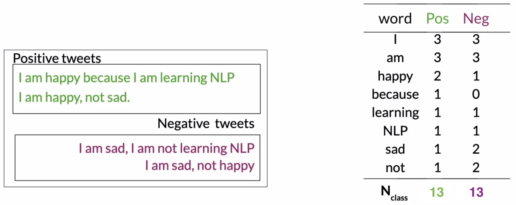
- Armed with two corpora, one with positive tweets and one with negative tweets, let’s look into the steps needed to generate our conditional probabilities table.
- Generate positive/negative frequency features: Extract the vocabulary (i.e., the unique words) that appear in both your positive and negative corpora along with their counts. In other words, we’re seeking to obtain the word-counts for each occurrence of a word in both the positive corpus and negative corpus, just like we did before with logistic regression.
- Note that the steps so far are common with what we’ve seen earlier with logistic regression.
- Fetch total counts: Get a total count of all the words in your positive corpus and negative corpus. That is, sum over the rows of the table below on the right-hand-side of the below figure. In this particular instance, for both positive and negative tweets, our total counts are 13 words.
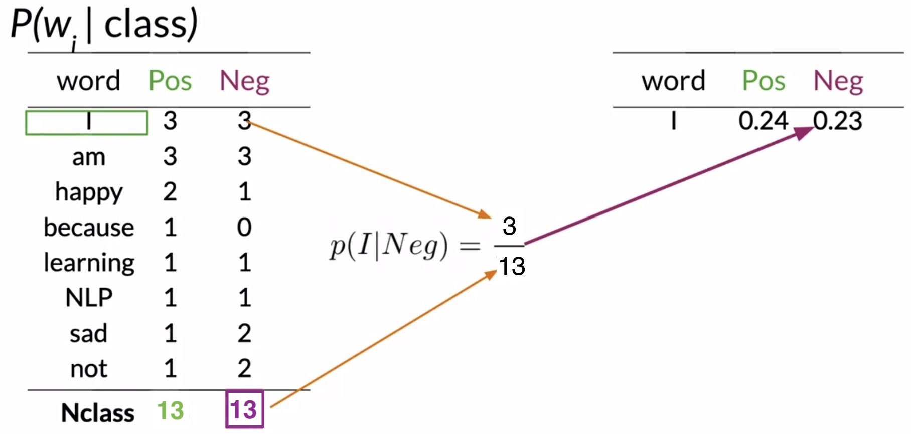
- Compute conditional probabilities given a class: Next, as the first new step for Naive Bayes, and it’s very important because it allows you to compute the conditional probabilities of each word given a class.
- This is obtained by dividing the frequency of each word in a class by its corresponding sum of words in the class.
- So for the word I, the conditional probability for the positive class would be \(\frac{3}{13} = 0.24\). Store this value in a new table that contains the conditional probabilities of each word in your tweet, as shown in the figure below.
- Similarly, for the word I, in the negative class, you get a conditional probability of \(\frac{3}{13} = 0.23\). Store that in your conditional probabilities table as well.
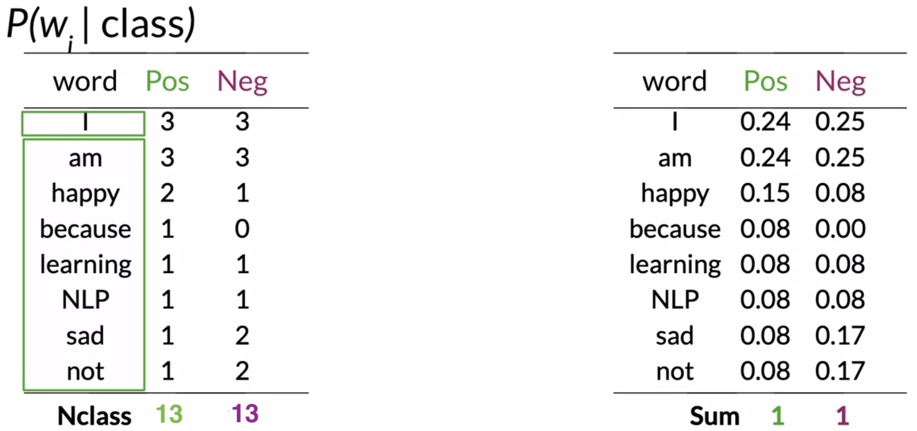
- Apply the same procedure for each word in your vocabulary to complete the conditional probabilities table.
These conditional probabilities basically represent how often the (unique) words in a tweet occur in positive and negative tweet samples.
- Sanity check your conditional probabilities: A key property of the conditional probabilities table is that if you sum over all the probabilities for each class, you’ll get 1, since \(\sum\limits_{i} P_i = 1\).
- Let’s investigate this table further to see what these numbers mean.
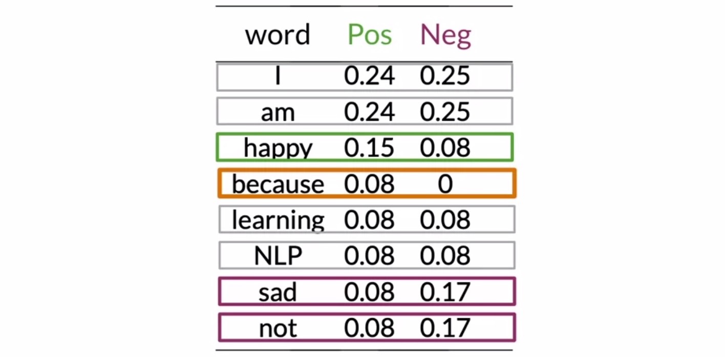
- First, note the words have a nearly identical conditional probability, viz., I, am, learning, and NLP. The interesting thing here is words that are equally probable don’t add much to the sentiment.
- In contrast to these neutral words, look at some of these other words like happy, sad, and not. They have a significant difference between probabilities. These are your power words tending to express one sentiment or the other. These words carry a lot of weight in determining your tweet sentiments.
- Now let’s take a look at because. Since, it only appears in the positive corpus, its conditional probability for the negative class is 0. When either of the probabilities (corresponding to the positive/negative classes) turn out to be 0, you have no way of comparing between the two corpora.
- To avoid this, you’ll need to smooth out your probability function, as described in the next section on Laplacian smoothing.
Laplacian smoothing
- For a particular word, the probability of a class being 0 leads to an issue for our downstream calculations, as follows:
- Consider the case where the negative-class probability for a particular word is 0. Because the negative-class probability resides in the denominator in our Naive Bayes inference equation, this leads to a divide-by-0.
- Similarly, if the positive-class probability for a particular word is 0, this will lead to the overall Naive Bayes inference expression zeroing out because the positive-class probability resides in the numerator.
- Let’s dive into Laplacian Smoothing, a technique you can use to avoid your probabilities being 0.
- The expression used to calculate the conditional probability of a word \(w_i\), given a class, is the frequency of the word in the corpus \(P(w_i|class)\) is given by \(\frac{freq(w_i, class)}{N_{class}}\). Smoothing the probability function means that you will use a slightly different formula from the original, as shown in the figure below.
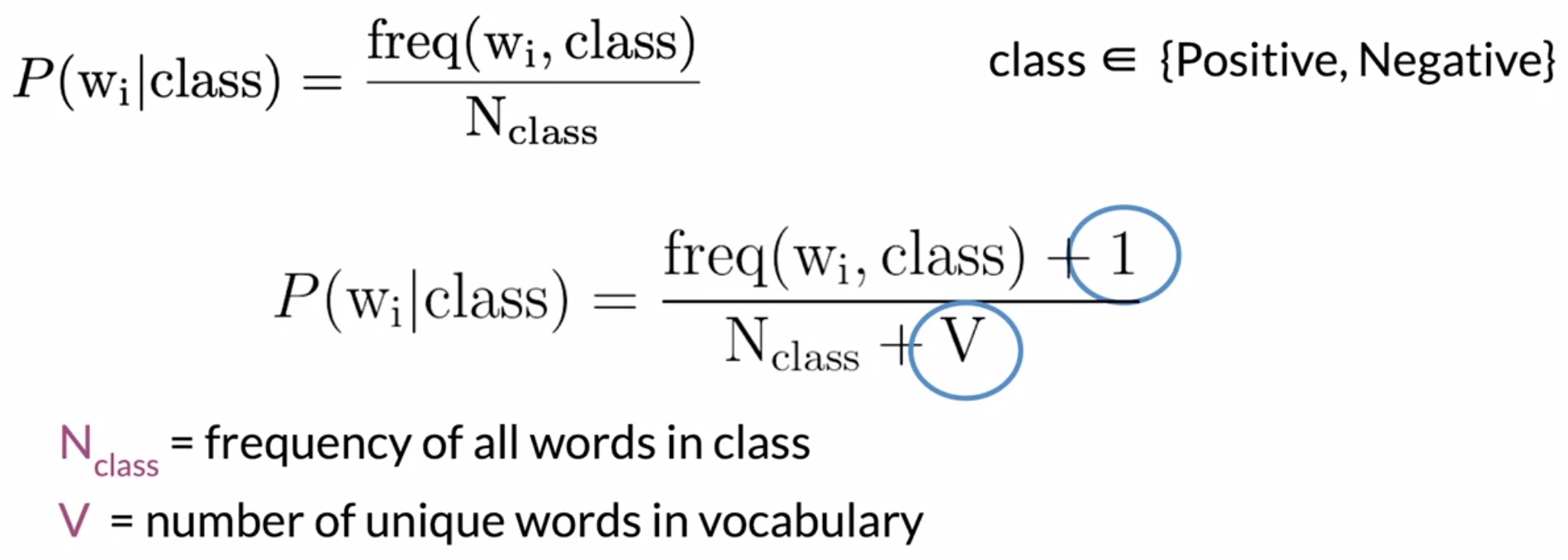
- Thus, to compute the positive and negative probability for a specific word \(w_i\) in the vocabulary, we have:
- where:
- \(freq(w_i, pos)\) and \(freq(w_i, neg)\) are the frequencies of word \(w_i\) in the positive and negative class respectively. In other words, the positive frequency of a word is the number of times the word is counted with the label of 1.
- \(N_{pos}\) and \(N_{neg}\) are the total number of positive and negative words for all documents/tweets respectively.
- \(V\) is the number of unique words in the entire dataset that encompasses all classes, positive and negative.
- Note that we’ve added a 1 to the numerator for additive smoothing, which is another name for Laplacian smoothing. This little transformation avoids the probability being 0. However, it adds a new term to all the frequencies that is not correctly normalized by \(N_{class}\). To account for this, we’ll need to add a new term \(V\) to the denominator In other words, adding \(V\) in the denominator helps account for the extra \(+1\) added to the numerator.
- Recall that your vocabulary \(V\) is the set of unique words in your corpora consisting of both the positive and negative tweets (i.e., the entire vocabulary and not just the unique words in a single class). So now all the probabilities in each column will sum to 1. This process is called Laplacian smoothing.
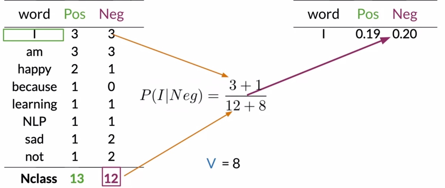
- Let’s consider an example below. Note how the probabilities are computed for both the positive and negative columns. Since the size of our vocabulary \(V\) is 8, we use \(V = 8\) for both the positive and negative cases in the denominator.
- Step 1: Calculate is the number of unique words in your vocabulary \(V\). In this particular e.g., you have 8 unique words.
- Step 2: Calculate the probability for each word in the positive and negative class.
- Consider the word I:
- For the positive class, you get \((3 + 1)/(13 + 8) = 0.19\).
- For the negative class, you have \((3 + 1)/(12 + 8) = 0.2\).
- … and so on for the rest of the table.
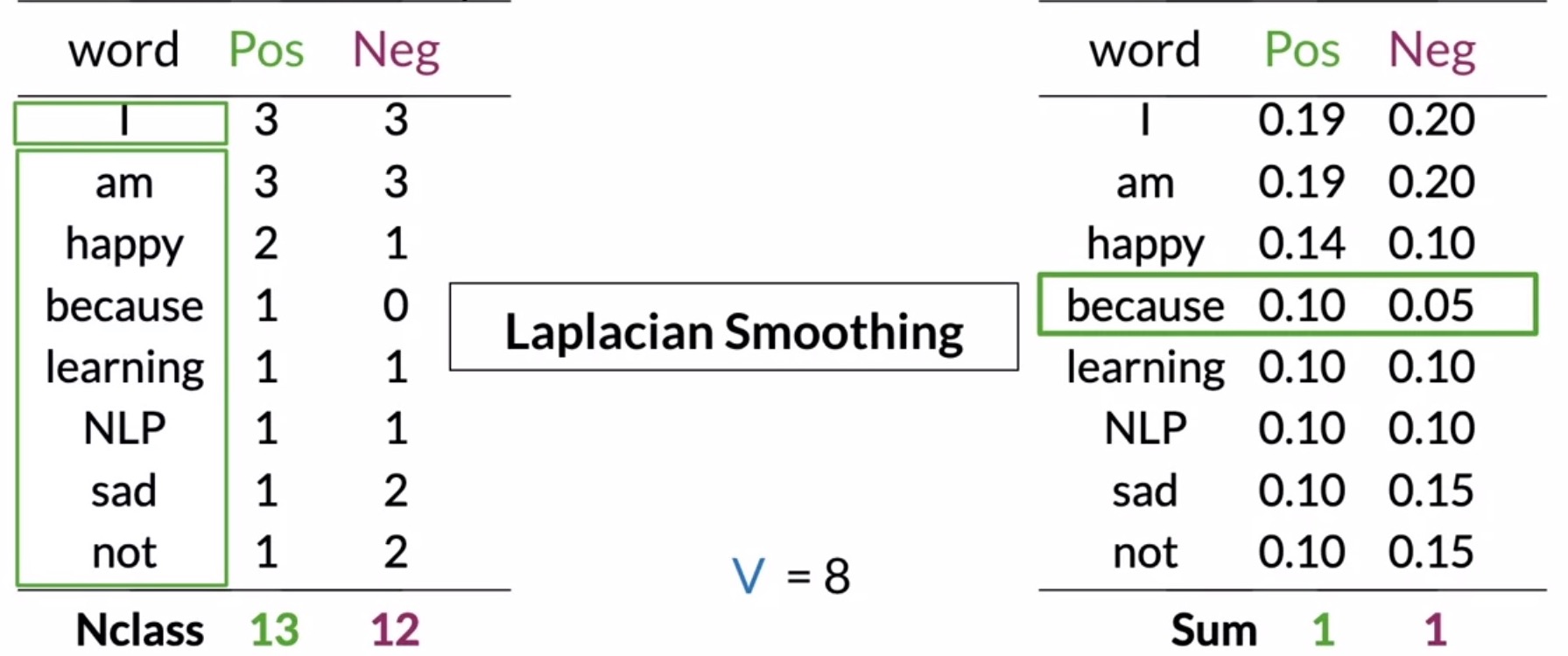
- The numbers shown here have been rounded, but using this method the sum of probabilities in your table will still be 1.
- Most importantly, note that the word because no longer has a probability of 0.
- Consider the word I:
- Shown below is the tabulation of the conditional probabilities for each word in \(V\) for the positive and negative class:
- Key takeaway
- Use Laplacian smoothing so your probabilities don’t end up being 0.
Naive Bayes
- In the previous module, we learned how to classify tweets using logistic regression. In this week, we’ll solve the same problem using a method called the Naive Bayes. It’s a reasonably good and easy-to-implement baseline for many text classification tasks, including sentiment analysis.
- Naive Bayes is an algorithm that falls under the domain of supervised machine learning, and relies on word frequency counts just like logistic regression.
The “naive” in Naive Bayes comes from the fact that this method makes the assumption that the features you’re using for classification are all independent, which in reality is rarely the case.
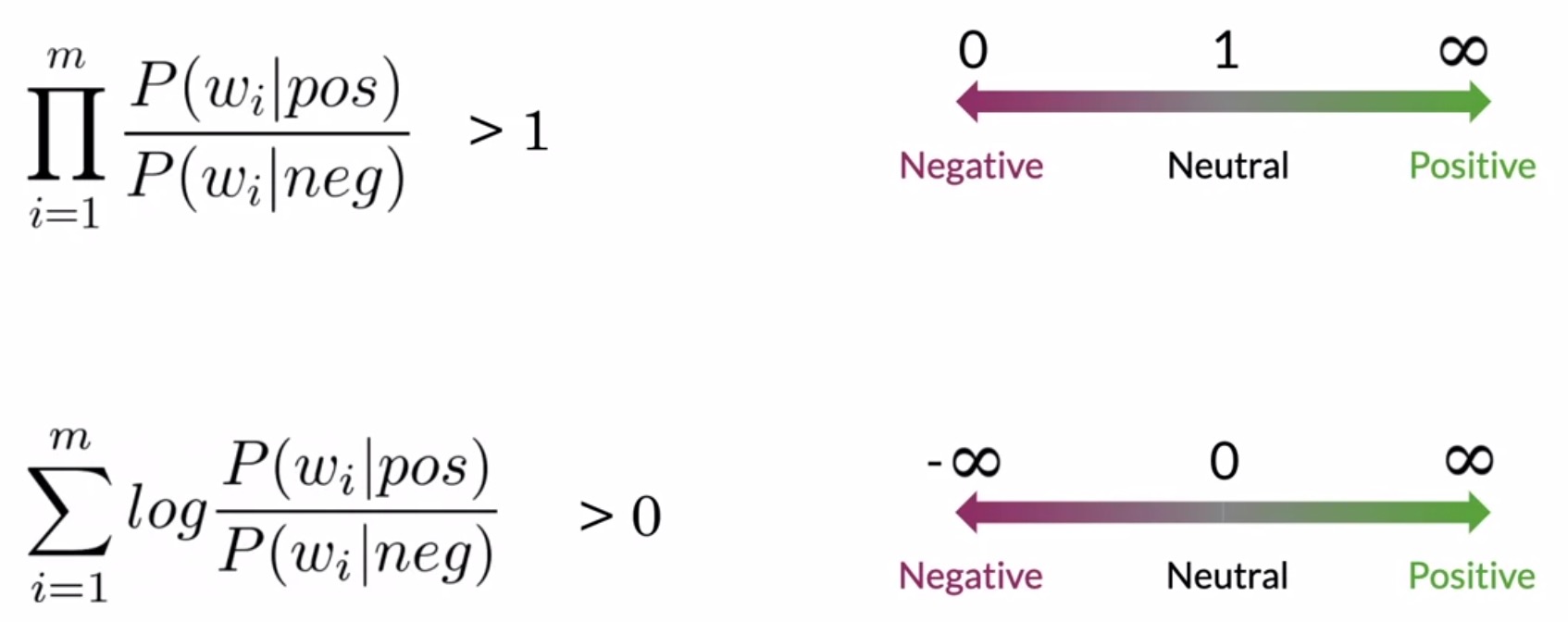
- Formally, the Naive Bayes inference condition rule for binary classification can be expressed as follows:
-
Dissecting this expression, you can see that we’re going to take the product (across all of the unique words in your tweets, i.e., your vocabulary) of the probability for each word in the positive class divided by its probability in the negative class.
-
Let’s apply the Naive Bayes inference condition rule for binary classification to an example, using the conditional probabilities table we derived in the prior section on computing the conditional probabilities table. Say your tweet says,
"I'm happy today, I'm learning". Using the table of conditional probabilities (after applying Laplacian smoothing), we can predict the sentiment of the whole tweet as shown below:
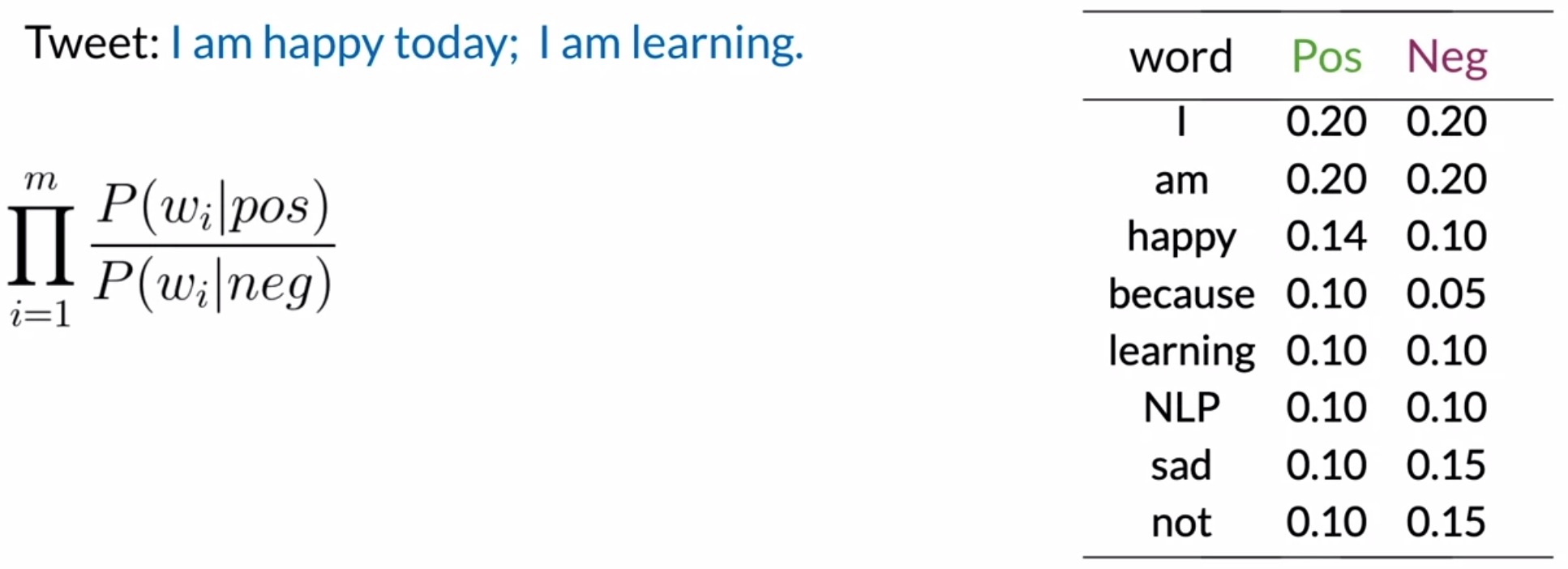
- Now, let’s calculate the Naive Bayes product for our tweet.
- For each word, select its probabilities from the table. So for I, you get a positive probability of \(0.2\) and a negative probability of \(0.2\). So the ratio that goes into the product is \(\frac{0.2}{0.2}\). Similarly, the ratios for the next words are as in the table below.
| Word | \(\frac{P(w_i|pos)}{P(w_i|neg)}\) |
|---|---|
| I | \(\frac{0.2}{0.2}\) |
| am | \(\frac{0.2}{0.2}\) |
| happy | \(\frac{0.14}{0.10}\) |
| today | \(-\) |
| I | \(\frac{0.2}{0.2}\) |
| am | \(\frac{0.2}{0.2}\) |
| learning | \(\frac{0.10}{0.10}\) |
- Note:
- Since there is no entry for today in our conditional probabilities table, this implies that this word is not in your vocabulary. So we’ll ignore its contribution to the overall score.
- All the neutral words in the tweet such as I and am cancel out in the expression, as shown in the figure below.
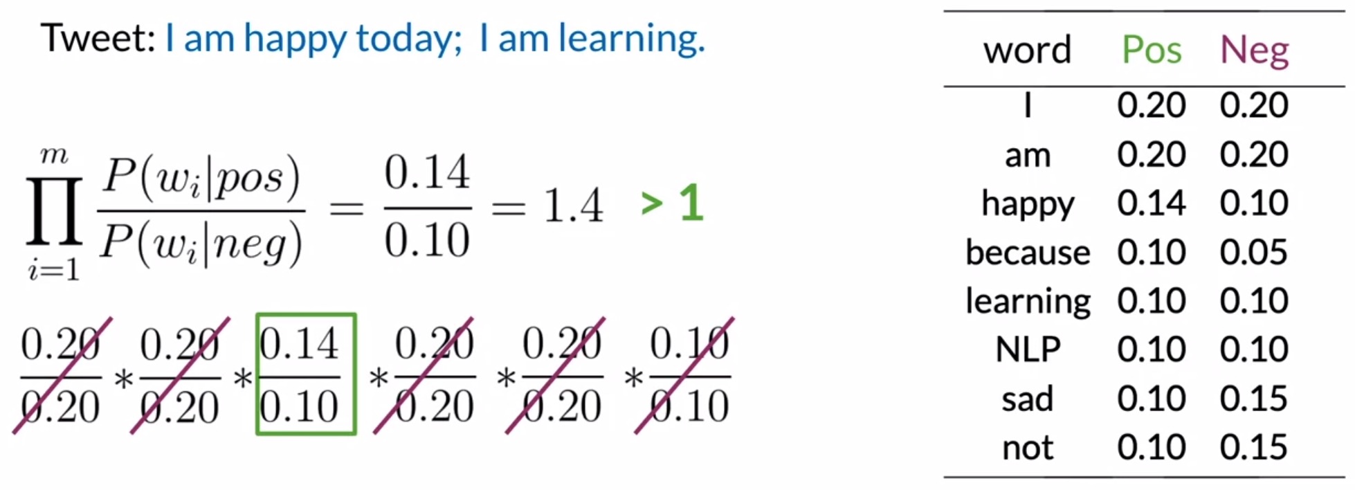
- Overall, what you end up with is \(\frac{0.14}{0.10} = 1.4\).
- Since this value is higher than 1, we can infer that the words in the tweet collectively correspond to a positive sentiment, so you conclude that the tweet is positive.
Background
Log likelihood
- Log likelihoods are just logarithms of the probabilities, like the (conditional) ones we calculated in the last section on computing the conditional probabilities table. Compared to raw probability numbers, they are much more convenient to work with and appear throughout deep-learning and NLP.
- Shown in the below figure is the the table we derived previously that contains the conditional probabilities of each word, for both classes, i.e., the positive or negative sentiment.
- Words can have many shades of emotional meaning. But for the purpose of sentiment classification, they’re simplified into three categories: neutral, positive, and negative.
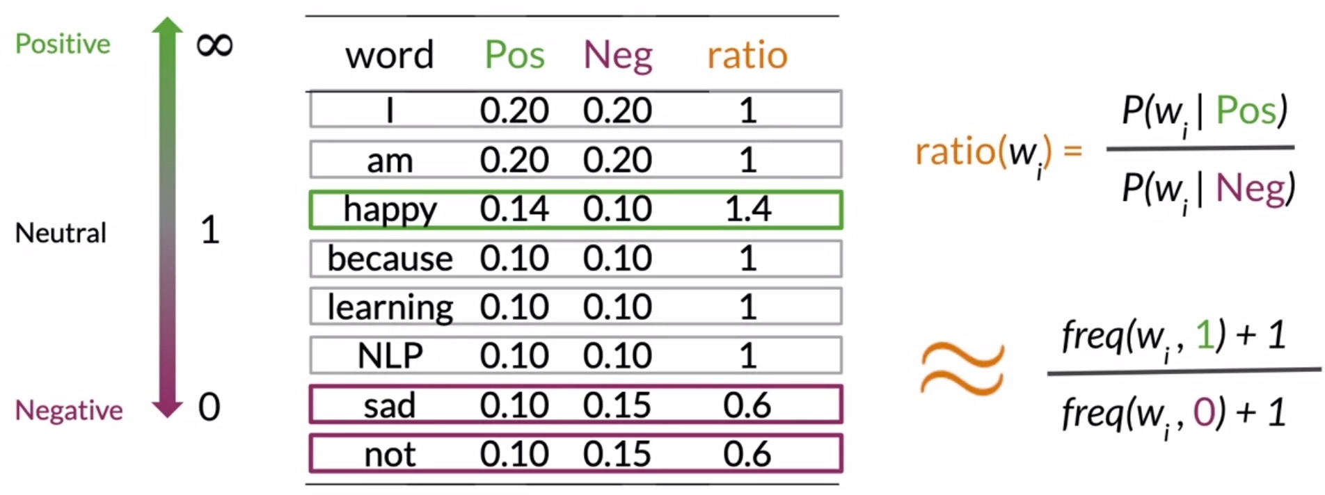
- Based on their conditional probabilities, we can identify the sentiment of a particular word \(w_i\). These classes/categories can be numerically estimated just by dividing the corresponding conditional probabilities of this table, as follows:
- Let’s see how this ratio looks for the words in your vocabulary.
- The ratio for the word i is \(\frac{0.2}{0.2} = 1.0\).
- The ratio for the word am, is again, \(\frac{0.2}{0.2} = 1.0\).
- The ratio for the word happy is \(\frac{0.14}{0.10} = 1.4\).
- The ratio for the words because, learning, and NLP, the ratio is 1.
- For sad and not, their ratio is \(\frac{0.10}{0.15} = 0.6\).
- Note that neutral words have a ratio near 1. Positive words have a ratio larger than 1.
The larger the ratio, the more positive the word is going to be. On the other hand, negative words have a ratio smaller than one. The smaller the value, the more negative the word.
- We can thus filter words depending on their positivity or negativity. These ratios are essential in Naive Bayes for binary classification.
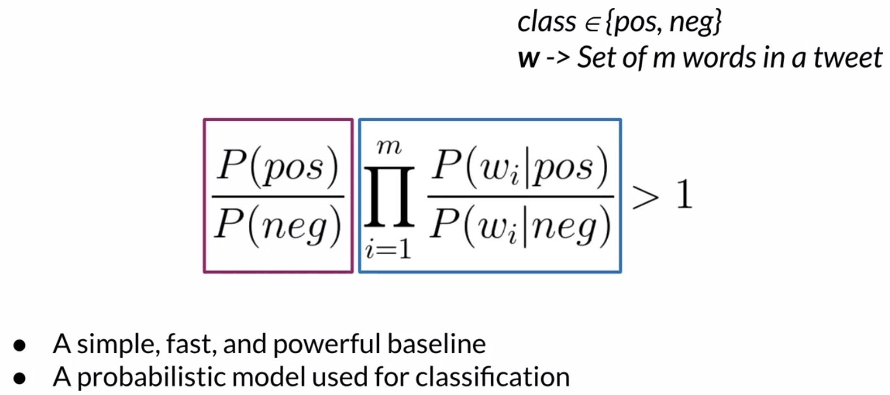
- Let’s illustrate this using an example. Recall that in Naive Bayes, you categorize a tweet as positive if the products of the corresponding ratios of every word appears in the tweet is larger than 1 and negative if it was less than 1. This is called the likelihood (boxed in blue in the figure below).
Log prior
- Let’s talk about the term boxed in purple in the figure above.
- For each class, estimate the probability of occurrence. In our case, we have two classes: positive and negative. Next, let’s assume:
- \(P(D_{pos})\) as the probability that the document/tweet is positive.
- \(P(D_{neg})\) as the probability that the document/tweet is negative.
- Note that \(P(pos)\) and \(P(neg)\) represent \(P(D_{pos})\) and \(P(D_{neg})\) in the above figure.
- where,
- \(D\) is the total number of documents/tweets.
- \(D_{pos}\) is the total number of positive tweets.
- \(D_{neg}\) is the total number of negative tweets.
- The prior is the ratio of the probabilities \(\frac{P(D_{pos})}{P(D_{neg})}\), which is effectively \(\frac{D_{pos}}{D_{neg}}\). Thus, the ratio of the number of positive to negative tweets is called the prior ratio.
- If you have exactly the same number of positive and negative tweets, the ratio is 1, which implies it needn’t be considered.
- However, when you have a positive-negative class imbalance (such datasets are called imbalanced), you need to accommodate the prior in your likelihood calculations.
- Intuitively, the prior probability represents the underlying probability in the target population that a tweet is positive versus negative. In other words, if we had no specific information and blindly picked a tweet out of the population set, the prior represents the probability that it will be positive versus negative.
- We can take the log of the prior to rescale it, and we’ll call this the log prior:
- Using the quotient rule of logarithms which states that \(log(\frac{A}{B}) = log(A)−log(B)\), the log prior can thus be calculated as the difference between the two log terms:
Preventing numerical underflow
- Another important consideration for your implementation of the Naive Bayes classifier is the possibility of a numerical underflow.
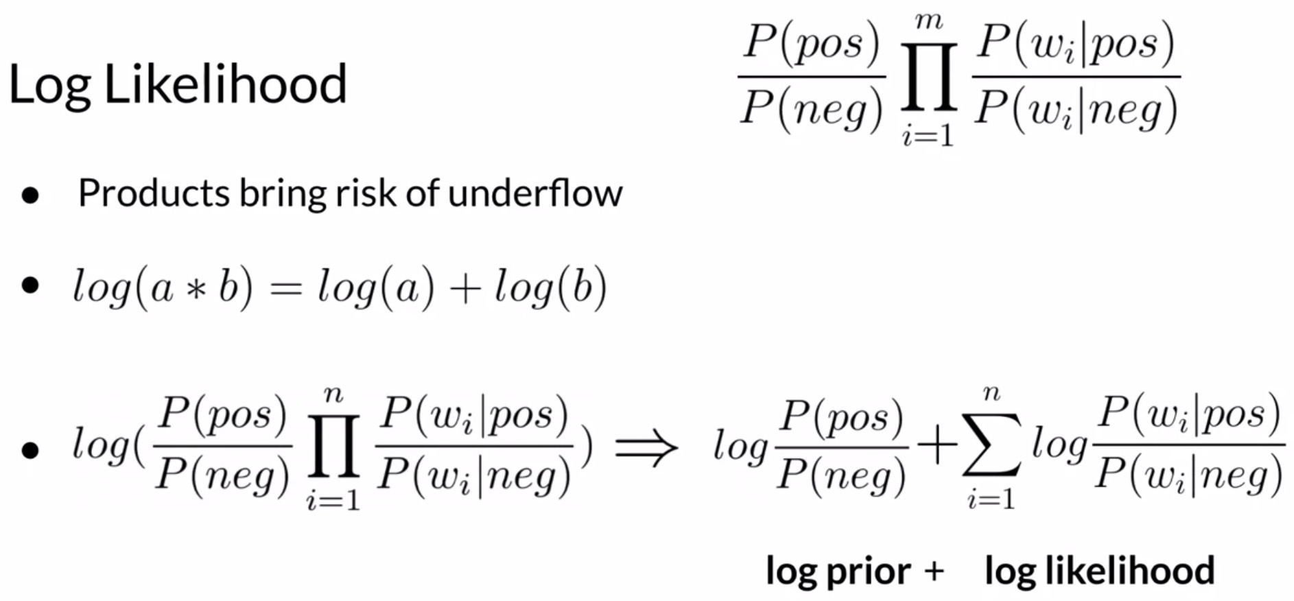
- Sentiment probability calculation requires multiplication of many numbers with values between \([0, 1]\). Carrying out such repeated multiplications runs the risk of numerical overflow since the magnitude of the result diminishes with every multiplication – in some cases, if the underlying hardware does not support the precision required to store such small magnitude numbers on the device.
- Luckily, there’s a mathematical trick to solve this which involves using a property of logarithms.
- Logarithms convert a product of numbers to an addition operation – this is referred to as the product rule in logarithms. This helps with the numerical underflow issues that we encounter when multiplying multiple small numbers in case of raw conditional probability ratios, because the multiplication operation is transformed to an addition. Formally, the product rule of logarithms states that:
Binary classification formulation
- Recall that the formula you’re using to calculate a score for Naive Bayes is the prior multiplied by the likelihood. The prior ratio coupled with the likelihood represent the full Naive Bayes formulation for binary classification, which is a simple, fast, and powerful method that you can use to establish a baseline quickly. Formally,
- Based on our discussions of using logs in the above section on preventing numerical underflow, let’s explore the trick of using the log of the likelihood score rather than the raw likelihood score. Recall that the likelihood score is essentially the ratio of the conditional probabilities corresponding to each of the possible classes.
-
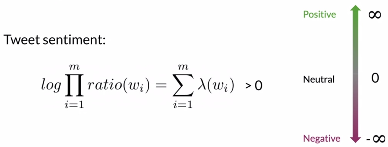
Owing to the product rule of logarithms, we may re-write the previous expression as the sum of the log prior and the log likelihood. Recall that the log likelihood itself is a sum of the logarithms of the conditional probability ratio of all unique words in your corpus. Formally,
\[p = \text{log prior} + \sum\limits_{i=1}^{N}{\text{log likelihood(} w_i \text{)}}\]- where,
- \(w_i\) represents a word in the tweet.
- \(N\) is the number of words in the tweet.
- where,
- The figure below summarizes the above ideas:
- Now, let’s use the method we’ve derived so far to classify the tweet,
"I'm happy because I'm learning". - Note that the values in the table here are unrelated to the previous dataset. It uses a bigger corpus and shows just a subset of the vocabulary, which is why we have lower probabilities and the sums per column doesn’t up to 1.
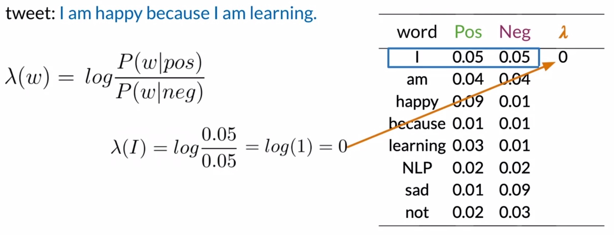
- Recall how we used the Naive Bayes inference condition earlier to get the sentiment score for your tweets. We’re going to do something very similar to get the log of the score, also known as the log likelihood, denoted by \(\lambda\). Formally,
- Now let’s calculate \(\lambda\) for every word in our vocabulary.
- For the word I, you get the logarithm of \(\frac{0.05}{0.05}\) or the logarithm of 1, which is equal to 0. Recall that the tweet will be labeled positive if the product is larger than 1.
- By this logic, I would be classified as neutral at 0.
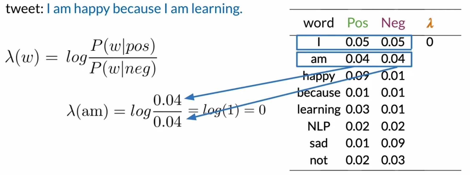
- For am, you take the log of \(\frac{0.04}{0.04}\), which again is equal to 0.
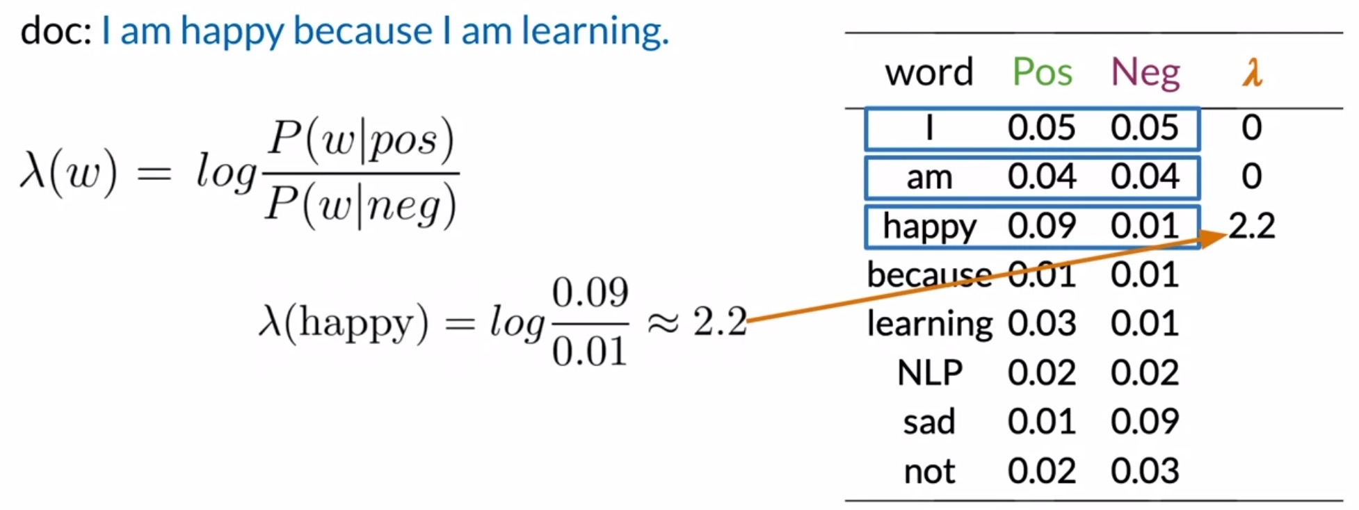
- For happy, you get a \(\lambda\) of \(2.2\), which is greater than 0, indicating a positive sentiment.
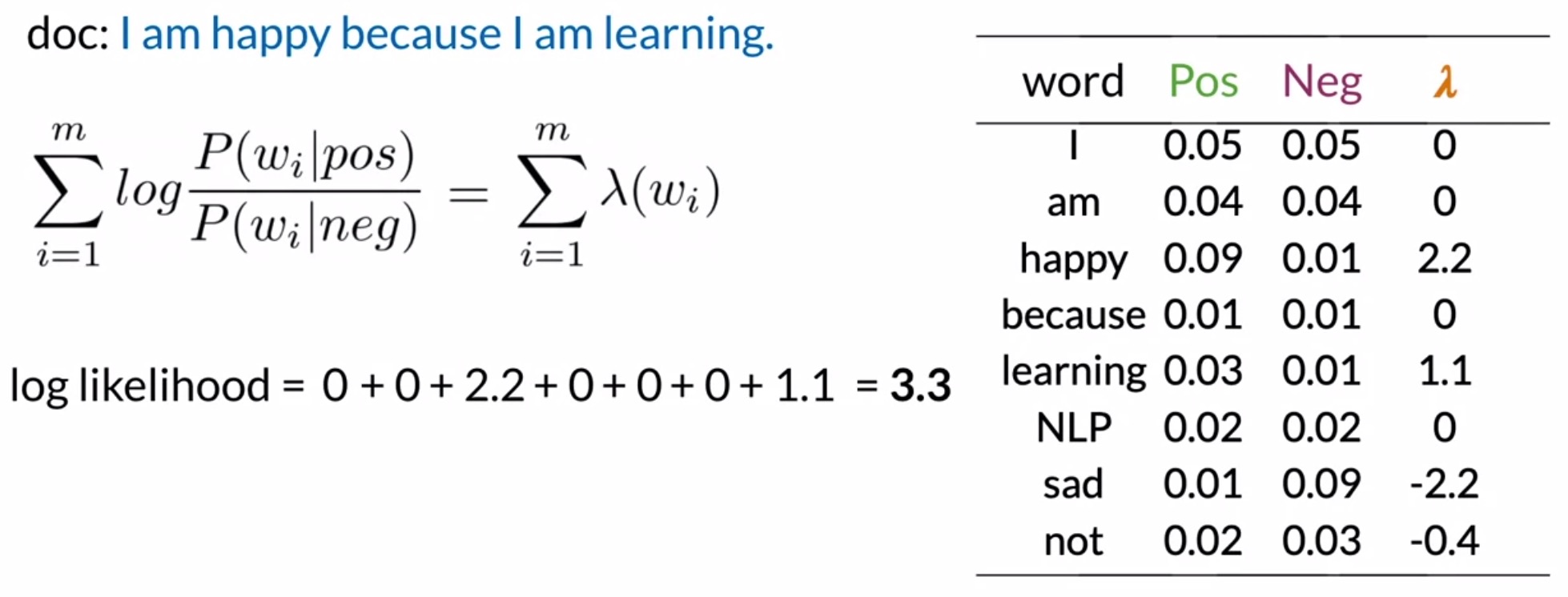
- From here on out, you can calculate the log score of the entire corpus just by summing out the \(\lambda\) terms.
- Thus, the log-likelihood of a tweet can be computed as the sum of the \(\lambda\) terms corresponding to each word in the tweet.
- Considering our example:
- For the word I, you add 0.
- For am, you add 0.
- For happy, you add \(2.2\).
- For because, I and am, you add 0.
- For learning, you add \(1.1\).
- The log-likelihood sum is \(3.3\).
- Recall that the tweet was positive if the product was larger than 1, and negative otherwise. With the log of 1 equal to 0, the positive values indicate that the tweet is positive. A value less than 0 would indicate that the tweet is negative.
- Since the log-likelihood for this tweet is \(3.3\), and this value is higher than 0, the tweet is marked positive.
-
Notice that this score is based entirely on the words happy and learning, both of which carry a positive sentiment. All the other words were neutral and didn’t contribute to the score. This shows the kind of influence power words have.
-
Key takeaways
- Words are often emotionally ambiguous but you can simplify them into three categories (neutral, positive, and negative) and measure exactly where they fall within those categories for binary classification.
- To do so, you divide the conditional probabilities of the words in each category/class.
- This ratio can be expressed as a logarithm and is denoted by \(\lambda\).
- Computing the log of the likelihood helps reduce the risk of numerical underflow (due to multiplying many small numbers \(«\,1\)).
- Predict the sentiment of a tweet by summing all the \(\lambda\) terms corresponding to each word that appears in the tweet. This score is called the log-likelihood.
- For log-likelihood, the decision threshold is 0 instead of 1 as with raw scores. Positive tweets will have a log-likelihood above 0, and negative tweets will have a log-likelihood below 0.
- Considering the log prior in case of unbalanced datasets, if \(\text{log likelihood + log prior > 0}\), then the tweet has a positive sentiment, or negative otherwise.
- Log-likelihoods make calculations simpler (since addition is simpler than multiplication, not only from a time-complexity perspective, but also a space-complexity perspective) and they also help with numerical stability.
Training Naive Bayes
- Let’s train the Naive Bayes classifier. Note that in this context, training has a slightly different meaning than in logistic regression or deep learning. There is no gradient descent, instead, we’re just counting frequencies of words in a corpus.
- The steps involved in training a Naive Bayes model for sentiment analysis are as follows.
- Gather data:
- For any supervised machine learning project, step 0 is to gather and label the data required to train and test your model.
- Annotate your dataset:
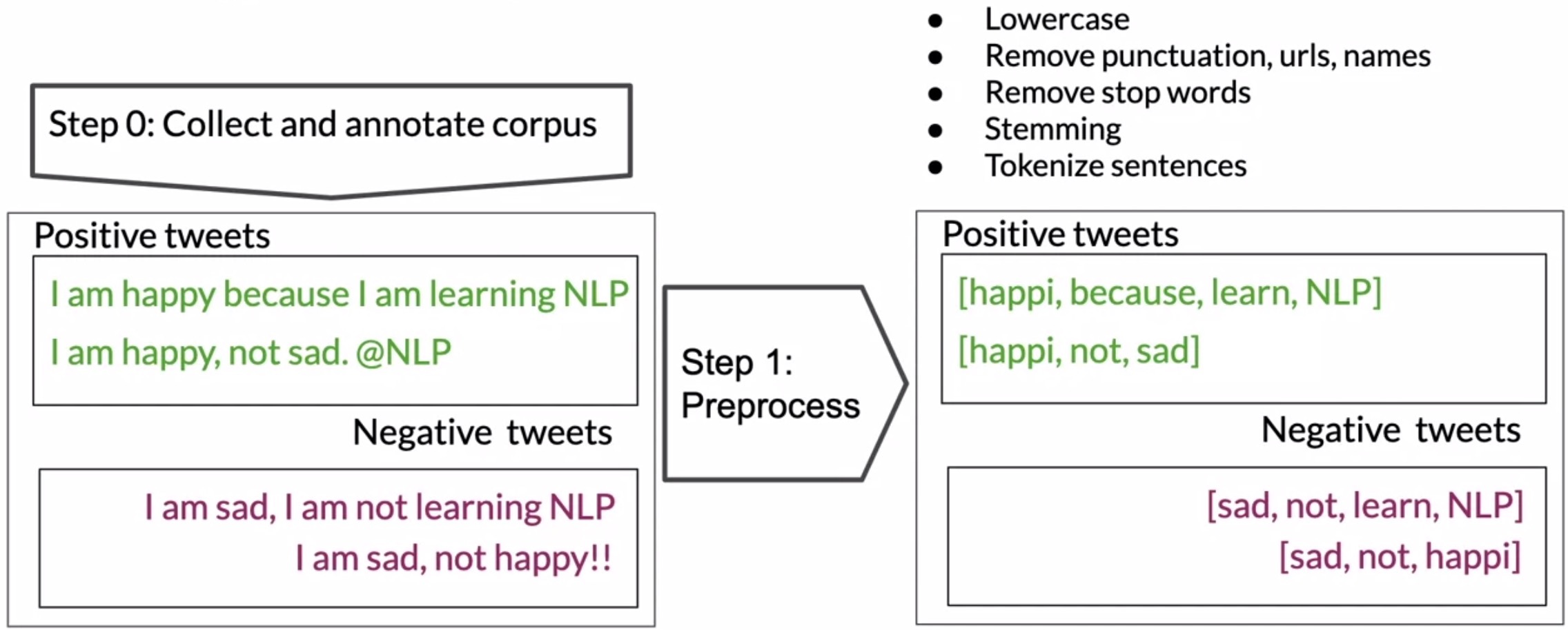
- For sentiment analysis of tweets, this step involves getting a corpus of tweets and annotating the dataset into two groups, positive and negative tweets.
- Preprocessing: The next step (shown in the figure below) is fundamental to your model’s success. The preprocessing step as described in the previous module, eliminates noise from your data by removing words that don’t offer the task at hand (in this case, sentiment analysis) relevant information about the content. These include all common words such as I, you, are, is, etc. that would not give us enough information on the sentiment. consists of five sub-steps:
- Lowercase
- Remove stop words and punctuation
- Remove task-specific stop words: URLs, handles etc.
- Stemming: reducing words to their common stem
- Tokenize sentences: splitting the corpus into single words or tokens.
- At the output of this step, we obtain a corpus of clean, standardized tokens.
- Note that it is relatively straightforward to implement this processing pipeline with simple ideas. However, in the real world, gathering and processing of data typically takes up a big chunk of the project’s timeline.
- The famous 80/20 rule of data science aptly summarizes this observation: “\(80\%\) of a data scientist’s valuable time is spent simply finding, cleansing, and organizing data, leaving only \(20%\) to actually perform analysis.”
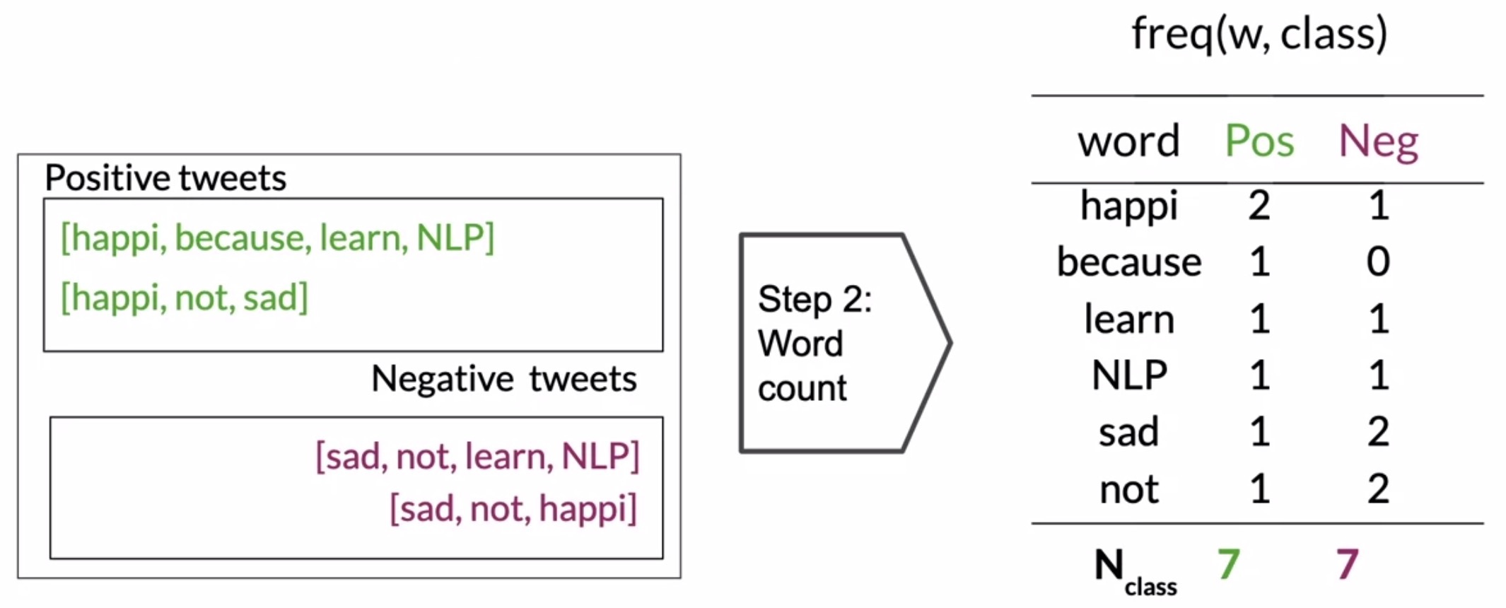
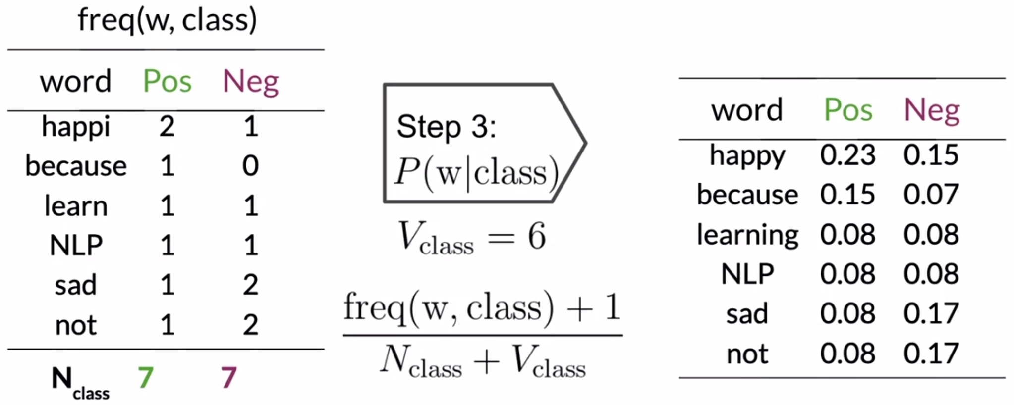
- Computing \(freq(w_i,class)\) for each word in your vocabulary: Once you have a clean corpus of tweets, obtain a vocabulary consisting of unique words in the corpora for each class. For each tuple of \((word, class)\), compute the frequencies similar to what we did with logistic regression. This will yield a table like the one shown in the figure here. Next, compute the sum of words and class in each corpus.
- Get probability ratios \(\frac{P(w|pos)}{P(w|neg)}\) using the Laplacian smoothing formula:
- From this table of frequencies, you get the conditional probability for a given class by using the Laplacian smoothing formula. As shown in the figure below, the number of unique words in \(V_{class}\) is 6.
- You only account for the words in the table, not the total number of words in the original corpus corresponding to that class.
- This produces a table of conditional probabilities for each word and each class, which only contains values greater than 0.
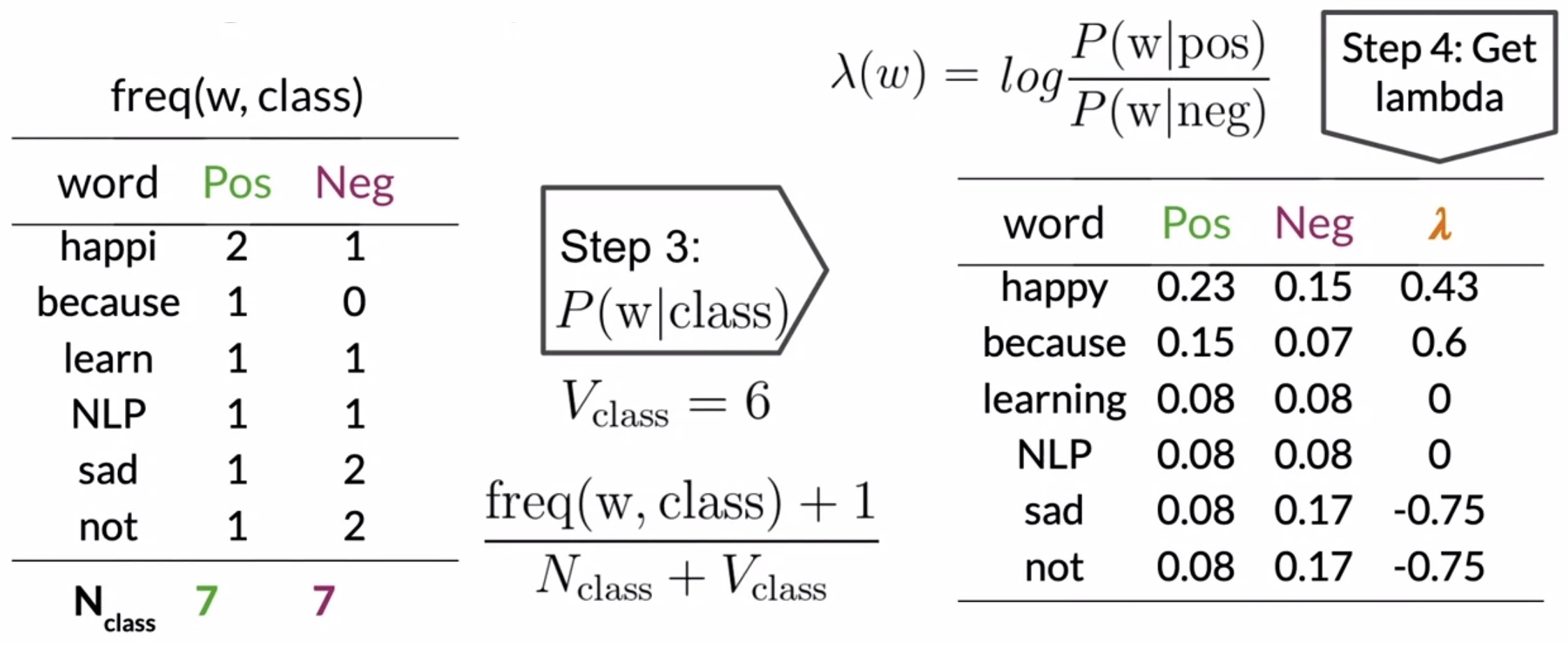
- Compute \(\lambda(w)\): Obtain the lambda score for each word, which is the log of the ratio of your conditional probabilities.
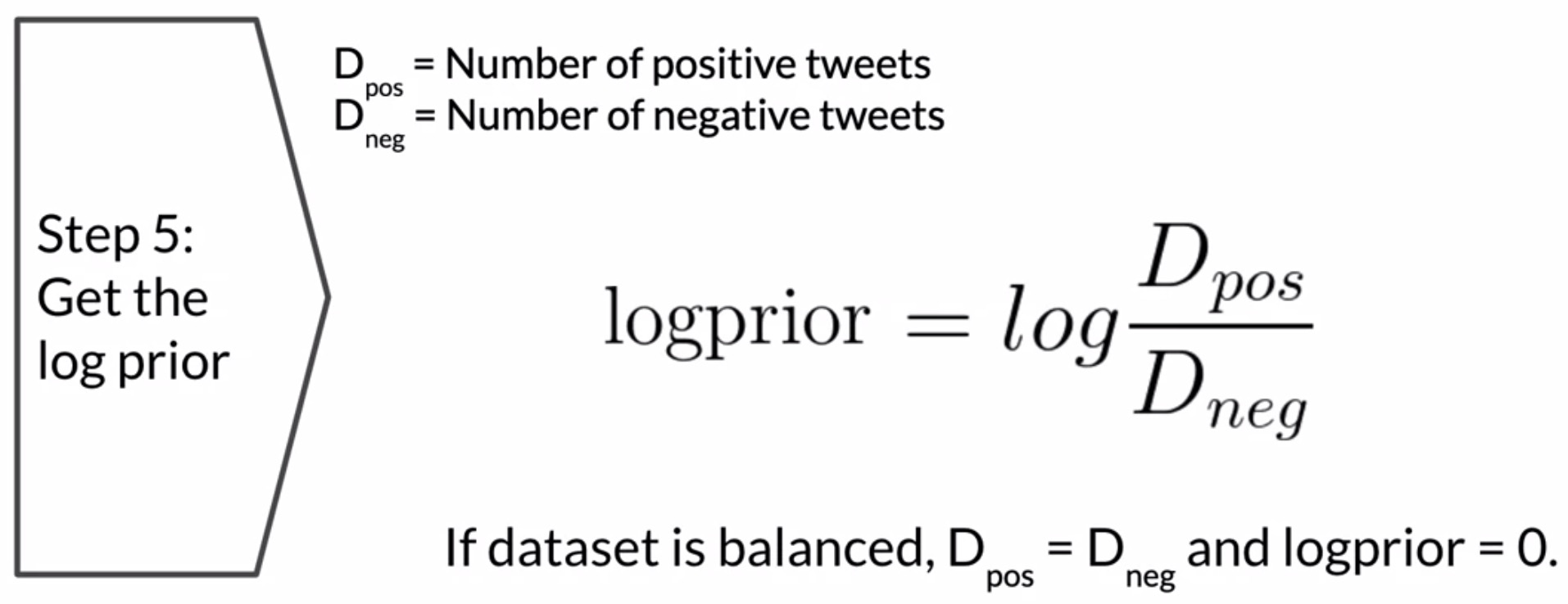
- Estimate \(\text{log prior} = \log\frac{P(pos)}{P(neg)}\): Calculate the log prior by counting the number of positive and negative tweets. The log prior is the log of the ratio of the number of positive tweets over the number of negative tweets. For balanced datasets, the log prior is 0. For unbalanced datasets, this term is important.
- Key takeaways
- Annotate a dataset with positive and negative labels for tweets.
- Pre-process the raw text to get a corpus of clean, standardized tokens.
- Compute the frequencies corresponding to each word and class (positive/negative) \(freq(w,class)\).
- Compute the conditional probabilities corresponding to each word and class \(P(w|pos); P(w|neg)\) using the frequencies computed in the prior step, and applying the Laplacian smoothing formula.
- Obtain the conditional probability ratio \(\frac{P(w|pos)}{P(w|neg)}\).
- Compute \(\lambda(w)\) or the log-likelihood score for each word.
- Finally, estimate the log prior of the model or how likely it is to see a positive tweet in your corpus.
Testing Naive Bayes
- Let’s work on applying the Naive Bayes classifier on validation examples to compute the model’s accuracy. Note that we shall cover some special corner cases.
- The steps involved in testing a Naive Bayes model for sentiment analysis are as follows.
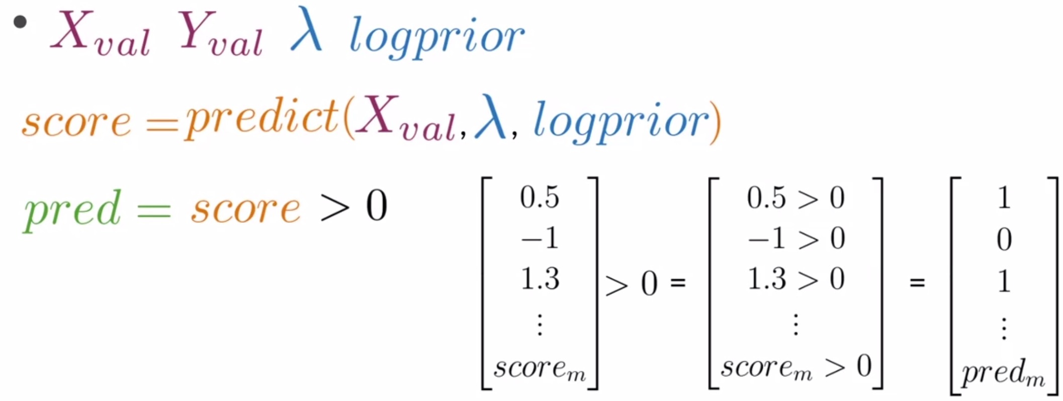
- Use the validation set: To evaluate/test the trained model, we take the conditional probabilities and use them to predict the sentiments of new unseen tweets, which in our case is the validation set of annotated tweets. The validation set includes data that was set aside during training and is composed of a set of raw tweets \(X_{val}\), and their corresponding sentiments, \(Y_{val}\).
- Pre-processing: Removing the punctuation, stemming the words, and tokenizing to produce a vector of words like this one.
- Compute the \(\lambda\) score for each unique word: Using the \(\lambda\) table (i.e., the log-likelihood table) for each unique word in our vocabulary, we compute the score for each word \(\lambda(X_{val})\) in the input sample.
- For words that have corresponding entries in the table, you sum over all the corresponding \(\lambda\) terms.
- Words that don’t show up in the log-likelihood table are considered neutral and don’t contribute anything to the overall score.
- Note that - Words that are not seen in the training set are considered neutral, and so add 0 to the score. your model can only give a score for words it’s seen before!
- Obtain the overall score: Summing up the scores of all the individual words, along with with our estimation of the log prior (important for an unbalanced dataset), we can predict the sentiment on a new tweet.
- Obtain the final prediction: The final prediction is \(score > 0\).
- Let’s consider an example tweet,
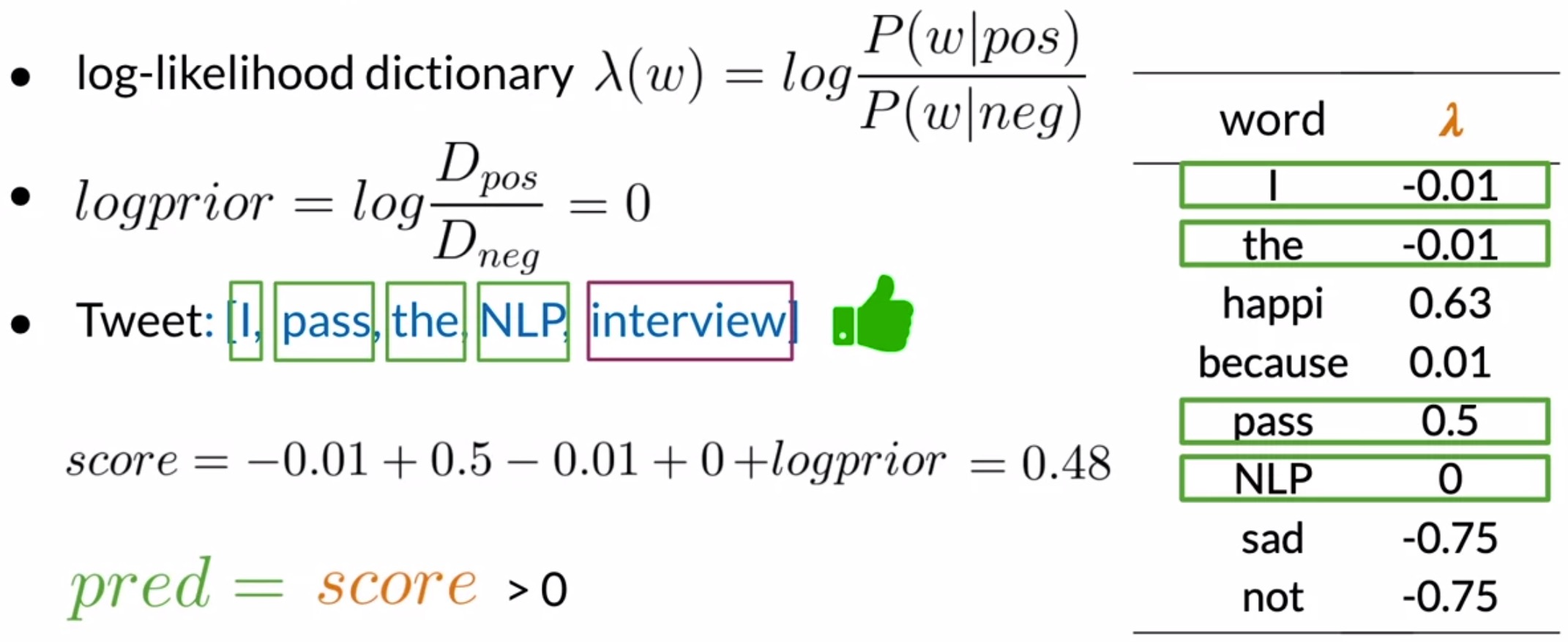
"I passed the NLP interview", and use our trained model to predict if this is a positive or negative tweet: - Look up each word from the vector in your log-likelihood table. Words such as I, pass, the, NLP have entries in the table, while the word interview does not (which implies that it needs to be ignored). Now, add the log prior to account for the imbalance of classes in the dataset. Thus, the overall score sums up to \(0.48\), as shown in the figure below.
- Recall that if the overall score of the tweet is larger than 0, then this tweet has a positive sentiment, so the overall prediction is that this tweet has a positive sentiment. Even in real life, passing the NLP interview is a very positive thing.
- To test the performance of our classifier on unseen data, we’ll need to implement an accuracy function to measure the performance of our trained model. To do so…
- Obtain the predictions for each entry in \(X_{val}\): Compute the score of each sample in \(X_{val}\), like you just did previously, then evaluates whether each score is greater than zero. This produces a vector populated with 0s and 1s indicating if the predicted sentiment is negative or positive for each tweet sample in the validation set, as shown below.
- Compute the prediction accuracy:
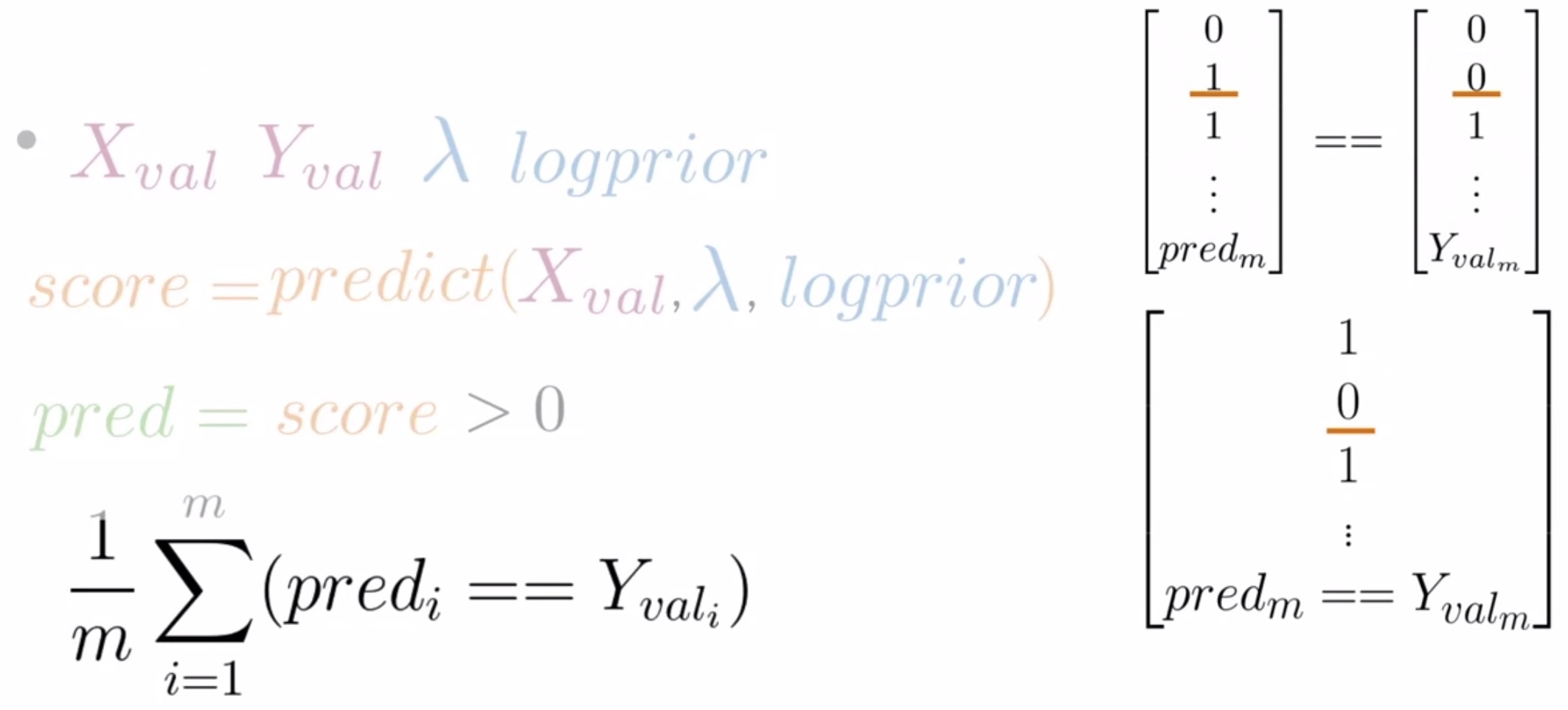
- With our new predictions vector, we can compute the accuracy of your model using the validation set. To do so, compare your predictions for each \(X_{val}\) against its ground truth \(Y_{val}\). If the values are equal and your prediction is correct, you will get a value of 1, and 0 otherwise.
- Once you have compared the values of every prediction with the true labels of your validation sets, you can compute the accuracy as the sum of this vector divided by the number of examples in the validation sets, as shown below. This is similar to what we did with logistic regression.
- Key takeaways
- To test the performance of your trained Naive Bayes model, use a validation set to predict the sentiment score for unseen tweets.
- Compared your predictions with ground truth labels provided as part of the validation set to calculate the accuracy of the model by identifying the proportion of tweets that were correctly predicted by your model.
- Words that don’t appear in the \(\lambda\) table are treated as neutral, and don’t add anything to the class score.
Applications
- Beyond sentiment classification, Naive Bayes lends itself to a plethora of applications.
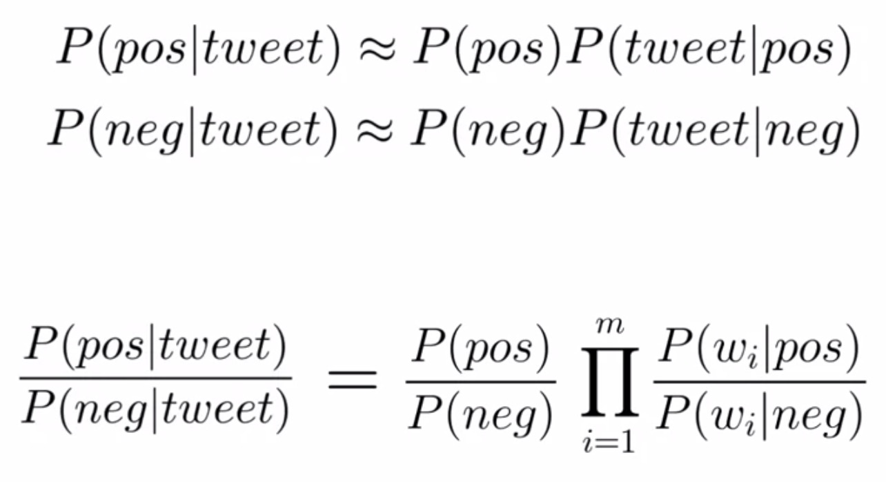
- When you use Naive Bayes to predict the sentiments of a tweet, what you’re actually doing is estimating the probability for each class using the joint probability of the words in the classes. The Naive Bayes formula states that the ratio between these two probabilities is given by the products of the priors and the likelihoods, as shown in the figure below. You can use this ratio between conditional probabilities for much more than sentiment analysis.
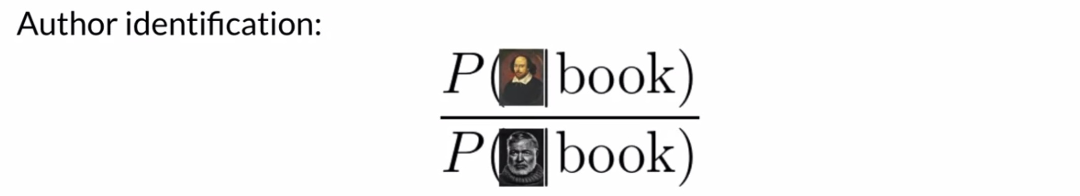
- Author identification: If you had two large corpora, each written by different authors, you could train the model to recognize whether a new document was written by one or the other. Suppose if you had some works by Shakespeare and some by Hemingway, you could calculate the \(\lambda\) for each word to predict how likely a new word is to be used by Shakespeare or Hemingway. This method also allows us to determine author identity.
- Spam filtering: Using information taken from the sender, subject and content, we can decide whether an email is spam or not.

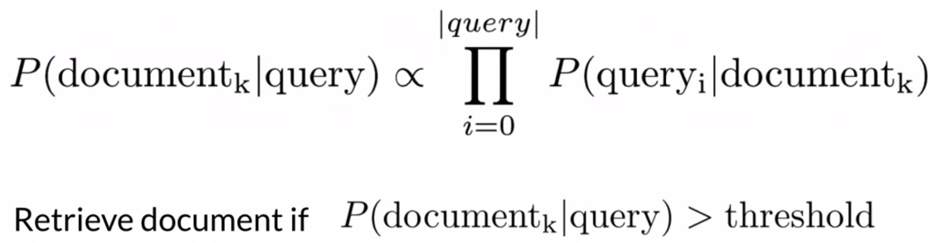
- Information retrieval: One of the earliest uses of Naive Bayes was filtering between relevant and irrelevant documents in a database. Given the sets of keywords in a query, in this case, you only needed to calculate the likelihood of the documents given the query. However, the challenge here is that you can’t know beforehand what a relevant or irrelevant document looks like. So you can compute the likelihood for each document in your dataset and then store the documents based on its likelihoods. You can choose to keep the first \(k\) results or the ones that have a likelihood larger than a certain threshold. Formally:
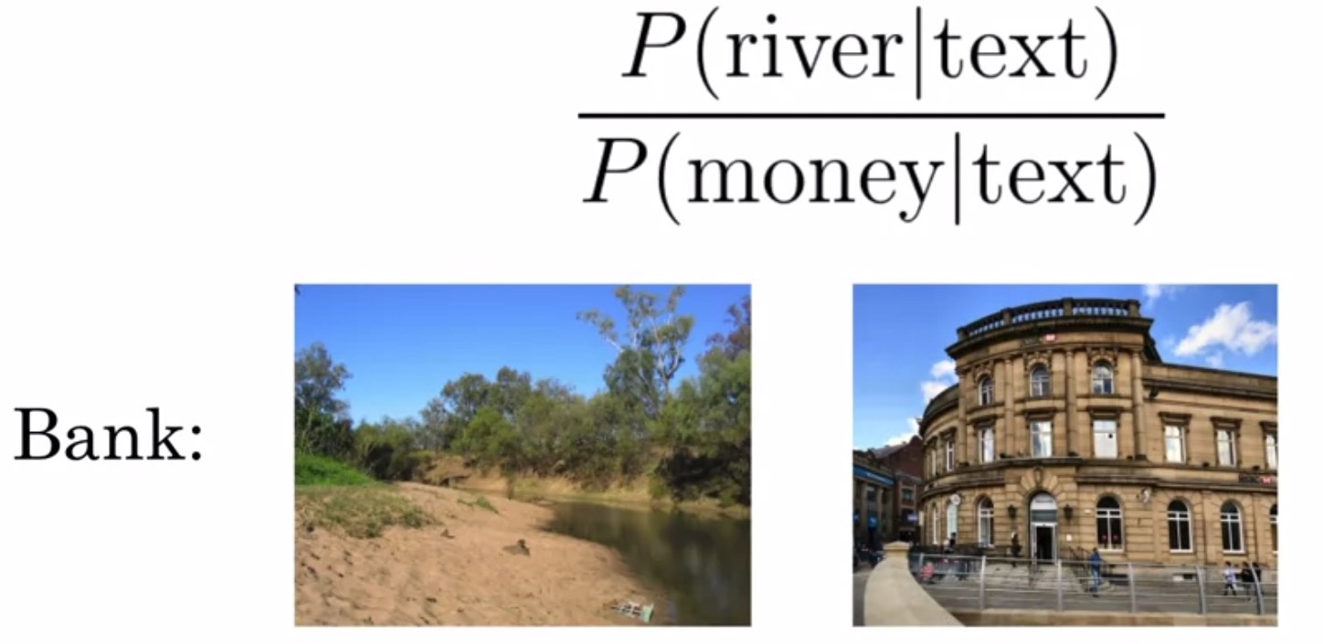
- Word disambiguation: Word disambiguation involves breaking down words for contextual clarity. Consider that you have only two possible interpretations of a given word within a text. Let’s say you don’t know if the word bank in your reading is referring to the bank of a river or to a financial institution. To disambiguate your word, calculate the score of the document, given that it refers to each one of the possible meanings. In this case, if the text refers to the concept of river instead of the concept of money, then the corresponding score \(P(river|text)\) will be larger than 1.
- Key takeaway
- Bayes Rule and it’s naive approximation has a wide range of applications. It’s a popular method since it’s relatively simple to train, use and interpret.
Assumptions
- Let’s understand the assumptions that underlie the Naive Bayes method.
- The primary assumption is the independence of features.
- Naive Bayes is a very simple model because it doesn’t require setting any custom parameters. This method is referred to as naive because of the assumptions it makes about the data. The first assumption is the independence between the predictors or features associated with each class and the second has to do with your validation set. Let’s explore each of these assumptions and understand how they could affect your results.
Independence
-
To illustrate the idea of independence between features, let’s consider the following sentence:
It is sunny and hot in the Sahara Desert. -
Naive Bayes assumes that the words in a sentence are independent of one another, but in reality, this typically isn’t the case. The word sunny and hot often appear together as they do in this example. Taken together, they might also be related to the location they’re describing, such as a beach or a desert. So the words in a sentence are not always necessarily independent of one another, but Naive Bayes assumes that they are. This could affect your estimation of the conditional probabilities of individual words.

- Let’s consider the task of sentence completion, given a sentence:
"It's always cold and snowy in ___", Naive Bayes might assign equal probability to the words spring, summer, fall, and winter even though from the context you can see that winter should be the most likely candidate. In the next modules of this specialization, we will look into sophisticated methods that can handle these cases better.

Relative Class Frequencies in Corpus
- Another issue with Naive Bayes is that it relies on the distribution of the training dataset, i.e., the proportion of the individual classes in the dataset.
- A good data set will contain the same proportion of positive and negative tweets as a random sample would. However, most available annotated corpora are artificially balanced for ease of analysis.
- In a real tweet stream, positive tweets occur more often than their negative counterparts.
- One reason for this is that negative tweets might contain content that is banned by the platform or muted by the user such as inappropriate or offensive vocabulary. Assuming that reality behaves as your training corpus, this could result in a skewed optimistic or pessimistic model.
- Thus, the relative frequency of the classes can affect the model’s performance if they are not representative of the real-world distribution.

- Key takeaways
- The assumption of independence in Naive Bayes is very difficult to guarantee, but despite that, the model works pretty well in certain situations.
- The relative frequency of positive and negative tweets in your training data sets needs to be balanced in order to deliver accurate results.
Error analysis
- Let’s delve into analyzing errors associated with cases where the model’s prediction didn’t turn out right and lead to a misclassified sentence, in our particular case of sentiment classification.
- There are several steps in the model’s pipeline where issues can lead to errors in the model’s prediction. Examples below:
- Incorrect preprocessing can lead to our model not being to able to clearly figure out the semantic meaning behind the input sentence.
- Word order drastically affects the meaning of a sentence.
- Some quirks of languages come naturally to humans, but confuse Naive Bayes models.
- Let’s delve into each of them one-by-one.
- Preprocessing
- One of your main considerations when analyzing errors in NLP systems should be what the preprocessed version of the text actually looks like.
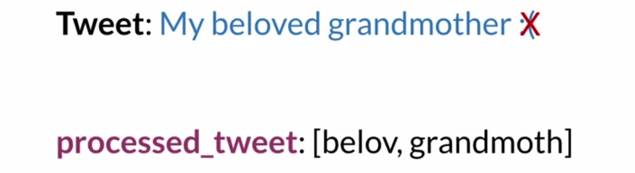
- Consider the tweet:
My beloved grandmother :(. - The sad face at the end of the tweet is very important to the sentiment of the tweet because it simply tells you the tweet carries a negative sentiment.
- If you’re removing punctuation, then the processed tweet will leave behind the stem-words associated with only
beloved grandmother, which appears to be a very positive tweet. - Similarly,
My beloved grandmother!would be a very different sentiment.
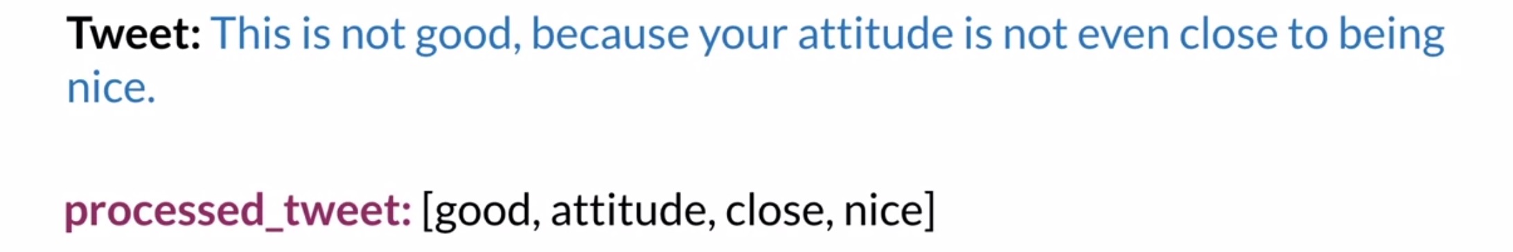
- Consider another example:
This is not good, because your attitude is not even close to being nice.- If you remove the neutral words such as not and this, what you’re left with is the following: Good, attitude, close, nice.
- From this set of words, any classifier will infer that this is something very positive.
- Word order
- The input pipeline isn’t the only potential source of trouble.
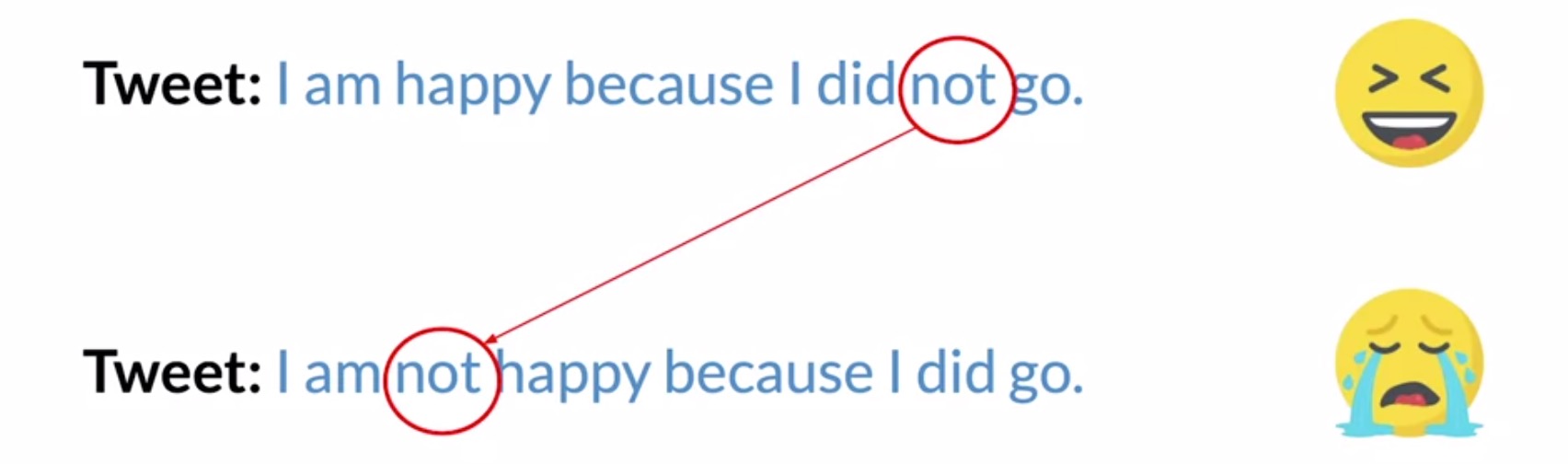
- Consider the tweet:
I'm happy because I did not go– this is a purely positive tweet. Now, consider another tweet:I'm not happy because I did not go, with a negative sentiment. - In this case, the not is important to the sentiment but gets missed by your Naive Bayes classifier.
- Thus, word order can be as important to spelling.
- Adversarial attacks
- A common pit-fall of Naive Bayes are adversarial attacks.
- The term adversarial attack describes some common language phenomenon like sarcasm, irony, and euphemism. Humans pick these up quickly but machines are terrible at it.
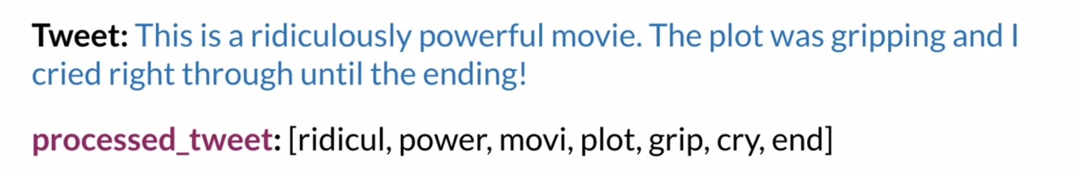
- Consider a tweet:
This is a ridiculously powerful movie. The plot was gripping and I cried right through until the ending.- The tweet contains a somewhat positive movie review, but pre-processing might suggest otherwise. If you pre-process this tweet, you’ll get a list of mostly negative words, but as you can see, they were actually used to describe a movie that the author enjoyed.
- Key takeaways
- Errors in a Naive Bayes-powered system can happen at the following locations in a typical model’s pipeline:
- Preprocessing
- Removing punctuation (example ‘:(‘)
- Removing stop words
- Word order
- E.g.:
I am happy because I did not govs.I am not happy because I did go
- E.g.:
- Adversarial attacks
- Easily detected by humans but algorithms are usually terrible at it!
- Sarcasm, Irony, Euphemisms, etc.
- E.g.:
This is a ridiculously powerful movie. The plot was gripping and I cried right through until the ending.
- Preprocessing
- Errors in a Naive Bayes-powered system can happen at the following locations in a typical model’s pipeline:
Further reading
Here are some (optional) links you may find interesting for further reading:
Citation
If you found our work useful, please cite it as:
@article{Chadha2020DistilledSentimentAnalysisUsingNaiveBayes,
  title   = {Sentiment Analysis using Naive Bayes},
  author  = {Chadha, Aman},
  journal = {Distilled Notes for the Natural Language Processing Specialization on Coursera (offered by deeplearning.ai)},
  year    = {2020},
  note    = {\url{https://aman.ai}}
}