Coursera-NLP • Sentiment Analysis using Logistic Regression
- Overview
- Supervised machine learning
- Sentiment analysis
- Feature extraction
- Preprocessing
- Tokenization
- Generating the features matrix
- Putting it all together in code
- Logistic regression as a classifier
- Further reading
- Citation
Overview
- Natural Language Processing (NLP) has changed a lot over the last several decades. The field has started off using primarily rule-based systems where someone might a rule like when you see the word good, assume this is a positive customer review. Next, came using probabilistic systems that perform much better, but still require a lot of hand engineering. Today, NLP relies much more on machine learning and deep learning.
- More recently with the rise of powerful computers, we can now train end-to-end systems that would have been impossible to train a few years ago. We can now capture more complicated patterns and we can use these models in question answering, sentiment analysis, language translation, text summarization, chatbots, etc.
- Many of these applications are built with attention models, which you are going to learn in this specialization. A few years ago, these models would take weeks or even months to train. But with attention, you can train these models in just a few hours.
-
In this specialization, you learn to build NLP technologies including the same technologies as what’s deployed in many large commercial systems.
- In course 1 of the Natural Language Processing Specialization offered by deeplearning.ai, you will:
- Perform (positive/negative) sentiment analysis of tweets using:
- Logistic regression
- Naive Bayes.
- Learn to represent words, queries and documents including other pieces of text as numbers in vectors. Use vector space models to discover relationships between words and use PCA to reduce the dimensionality of the vector space and visualize those relationships.
- Write a simple English to French neural machine translation algorithm using pre-computed word embeddings. Learn about locality sensitive hashing to relate words via approximate k-nearest neighbor search, to make the process of searching more efficient.
- Perform (positive/negative) sentiment analysis of tweets using:
- Pre-requisites: Python programming, basic knowledge of machine learning, matrix multiplications, and conditional probability.
Supervised machine learning
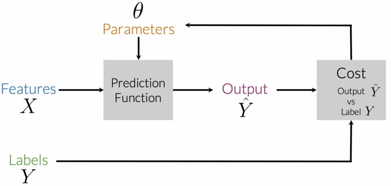
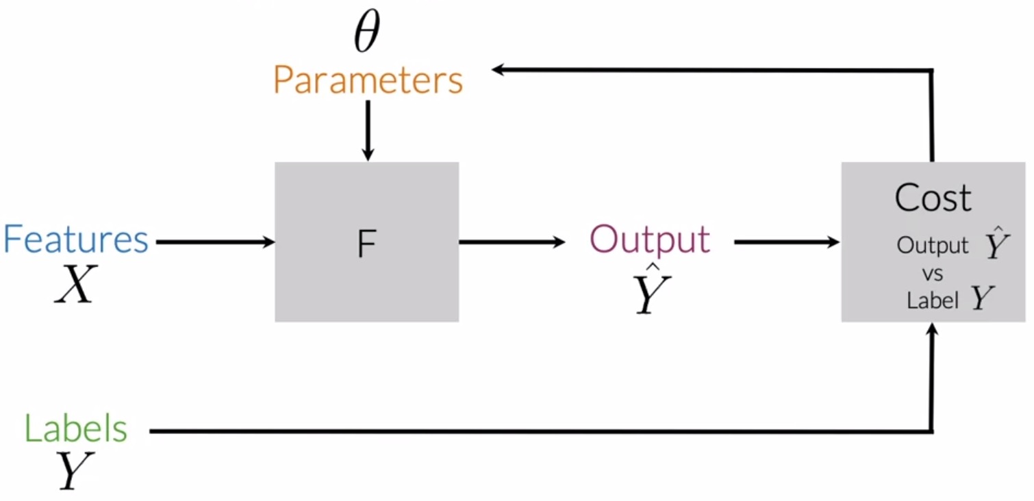
- In supervised machine learning, you have input features \(X\) and a set of labels \(Y\).
- To make sure you’re getting the most accurate predictions based on your data, the goal is to minimize your error rates or cost as much as possible.
- To do this, run the prediction function which takes in parameters to map your features to output labels \(\hat{Y}\).
- The best mapping from features to labels is achieved when the difference between the expected values \(Y\) and the predicted values \(Y\) is minimal.
- The cost function does this by comparing how closely the output \(\hat{Y}\) is to the label \(Y\).
- Update your parameters and repeat the entire process until your cost is minimized to convergence.
Sentiment analysis
- In sentiment analysis, the objective is to predict whether a body of text, say a tweet, has a positive or a negative sentiment.
- For e.g., let’s say you have 1,000 product reviews. Sentiment analysis lets you build a system to automatically go through all of these product reviews to figure out what fraction of them are positive reviews vs. negative reviews.
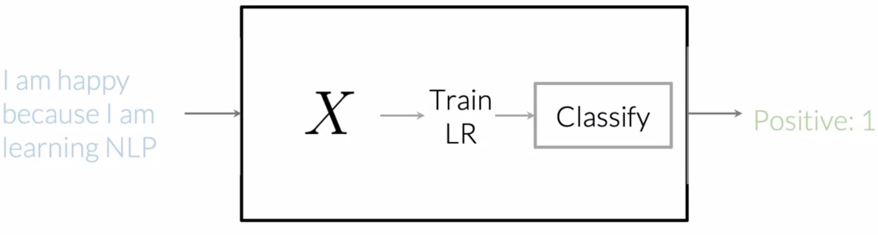
- Let’s model sentiment analysis as a supervised machine learning classification task using logistic regression.
- Building a logisitic regression classifier that performs sentiment analysis on tweets can be done in 3 steps:
- Extract features: process the raw tweets in the training set and extract useful features.
- Tweets with a positive sentiment have a label of 1, while those with a negative sentiment have a label of 0.
- Train: Train your logistic regression classifier while minimizing the cost.
- Predict: Come up with predictions using your learned model.
- Extract features: process the raw tweets in the training set and extract useful features.
- For implementation purposes, Natural Language Toolkit (NLTK) is a popular open-source Python library for natural language processing. It offers modules for collecting, handling, and processing Twitter data and much more.
Feature extraction
Sparse representations
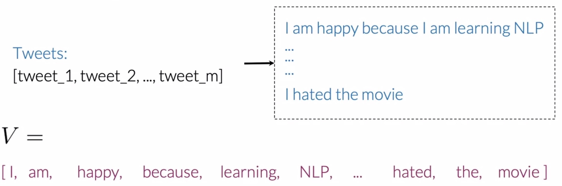
- To represent text as a vector, we need a vocabulary \(V\) that allows us to encode any body of text as a vector, more broadly, as an array of numbers.
- The vocabulary \(V\) would be the list of unique words from your list of tweets.
- Building such a list requires going through all the words from all your tweets and saving every new word that appears in your search.
- In the example below, you would have the word I, then the word, am, then, happy, and so forth.
- Note that in this case, the word I and the word am would not be repeated in the vocabulary (since a vocabulary only holds unique words).
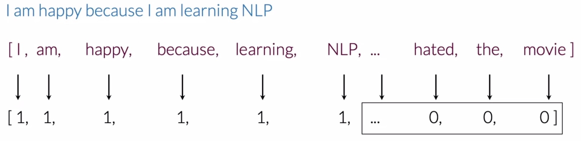
- To extract features using your vocabulary \(V\) with sparse representation, you would have to check if every word from your tweet appears in the vocabulary.
- If it does, like in the case of the word I, you would assign a value of 1 to that feature. If it doesn’t appear in the vocabulary, you would assign a value of 0.
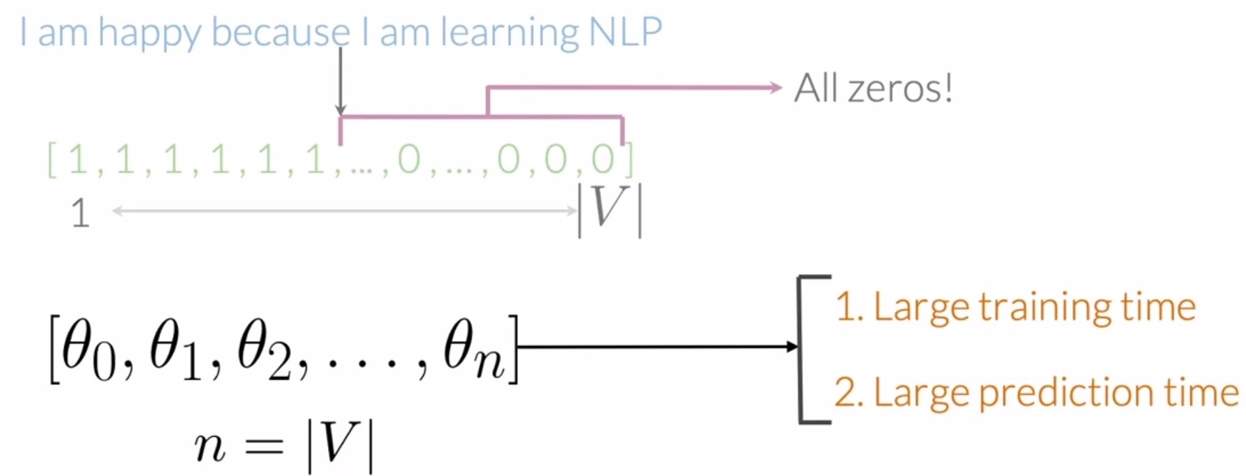
- In the below example, the representation of our sample tweet would have 6 ones and many zeros, which correspond to every unique word from your vocabulary that isn’t in the tweet.
- This type of representation with a relatively small number of non-zero values is called a sparse representation, as shown below.
- (-) Sparse representation leads to inefficiencies during training and testing: The number of features in a sparse representation is equal to the size of your entire vocabulary \(V\). This implies that a lot of features would be equal to 0 for every tweet. With the sparse representation, a logistic regression model would have to learn \(n + 1\) parameters, where \(n\) would be equal to the size of your vocabulary \(V\). For large vocabulary sizes, this would make your model inefficient in terms of training and inference/prediction/test time.
- For e.g., the number of parameters that a logistic regression classifier would have to learn using spare representations for feature extraction for the below inputs is 14.
[“I am happy because I am learning NLP”, “I hated that movie”, “I love working at DL”]
- Summary:
- Given some text, you can represent this text as a vector of dimension \(V\) by extracting features. Specifically, you did this for a tweet and you were able to build a vocabulary of dimension \(V\).
- As \(V\) gets larger, your training and inference/prediction/test time scales accordingly.
Negative and positive frequencies
- Frequencies (or counts) can serve as features into your logistic regression classifier. Specifically, given a word, you want to keep track of the number of times it shows up in a particular class.
- Let’s build two classes:
- A class associated with positive sentiment and,
- Another class associated with negative sentiment.
- To get the positive frequency for a word in your vocabulary, count the number of times it appears in the positive tweets. Correspondingly, obtain the negative frequency for a word by counting the number of times it appears in the negative tweets.
- Remember to sum the frequencies of unique words, and not duplicates.
-
Using both those counts, extract features and feed them into your logistic regression classifier.
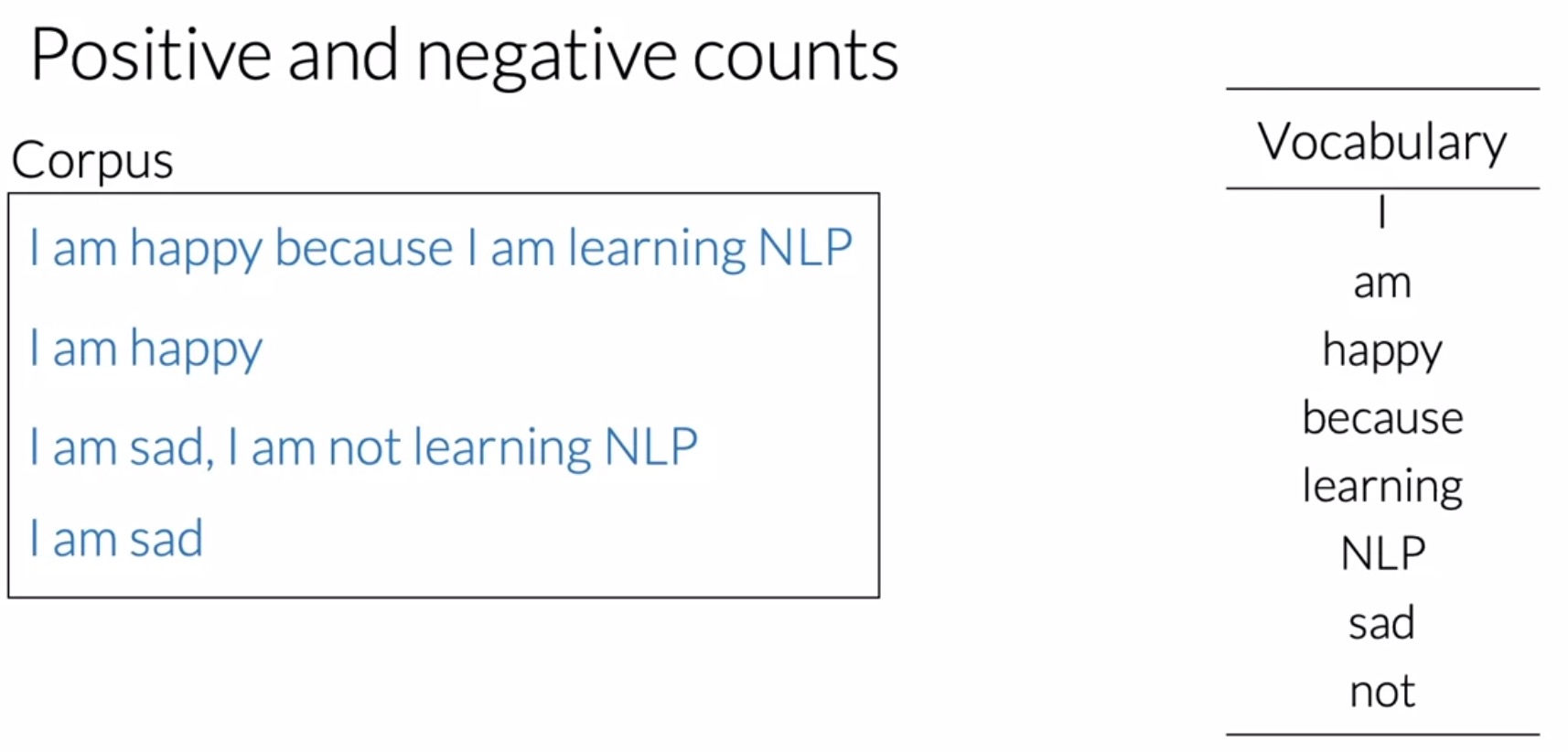
- As an e.g., consider a corpus consisting of four tweets as shown below. Associated with that corpus, you would have a set of unique words, i.e., your vocabulary \(V\). In the example below, your vocabulary \(V\) has eight unique words, as shown below.
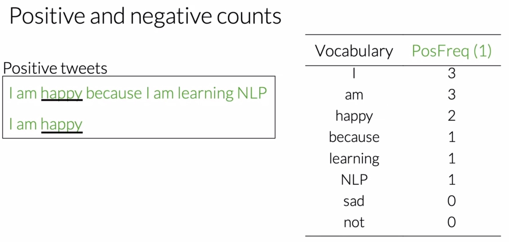
- For your corpus above, you have a set of two tweets that belong to the positive class, and a sets of two tweets that belong to the negative class. To get the positive frequency in any word in your vocabulary, you will have to count the times as it appears in the positive tweets. For instance, the word happy appears one time in the first positive tweet, and another time in the second positive tweet, making it’s positive frequency 2. Shown below is the positive frequency table (i.e., the positive count table).
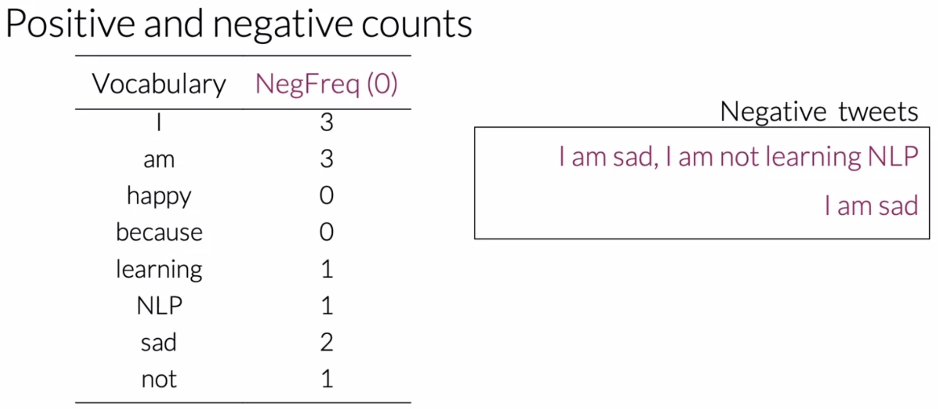
- Similarly, to obtain negative frequencies, consider the word am which appears 2 times in the first tweet and another time in the second one. So it’s negative frequency is 3. Shown below is the overall negative frequency table.
- The table below encapsulates the positive and negative frequencies for your sample corpus. In practice, when coding, this table is a dictionary mapping from a (word, class) pair to its frequency. This represents a frequency dictionary/hash-table, which maps a word and a class to the number of times that word showed up in the corresponding class.

- Thus, a frequency dictionary basically maps the following relationship:
Feature extraction with frequencies
- Recall that…
- The frequency of a word in a class is simply the number of times that the word appears on the set of tweets belonging to that class.
- The table summarizing this information is basically a dictionary mapping from (word, class) pairs to frequencies. Put simply, it tells us how many times each word showed up in its corresponding class.
- Using sparse representations, you learned to encode a tweet as a vector of dimension \(V\).
- Using negative and positive frequencies, you can encode a tweet by representing as a vector of dimension 3. This makes your logistic regression classifier faster, because instead of learning \(V\) features, you only have to learn 3 features.
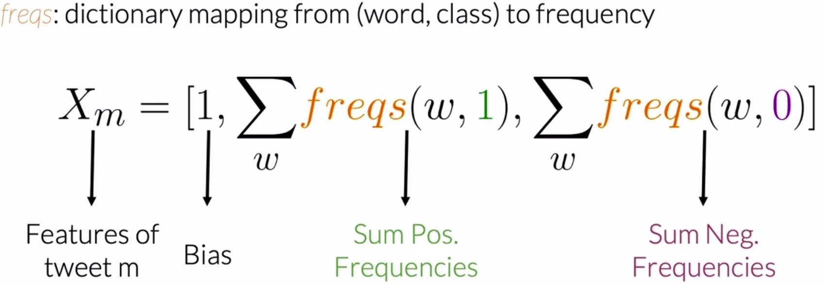
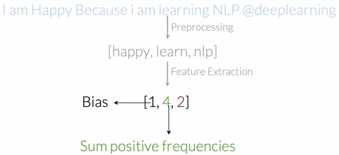
- As an e.g., lets consider an arbitrary tweet \(t\), shown below. Below are the list of features for this sample \(t\):
- First: bias unit equal to 1.
- Second: sum of the positive frequencies for every unique word in \(t\).
- Third: sum of negative frequencies for every unique word in \(t\).
- Thus, to extract features for this representation, you would only have to sum frequencies of words, which can be easily accomplished using the frequency dictionary concept we introduced in the prior section.
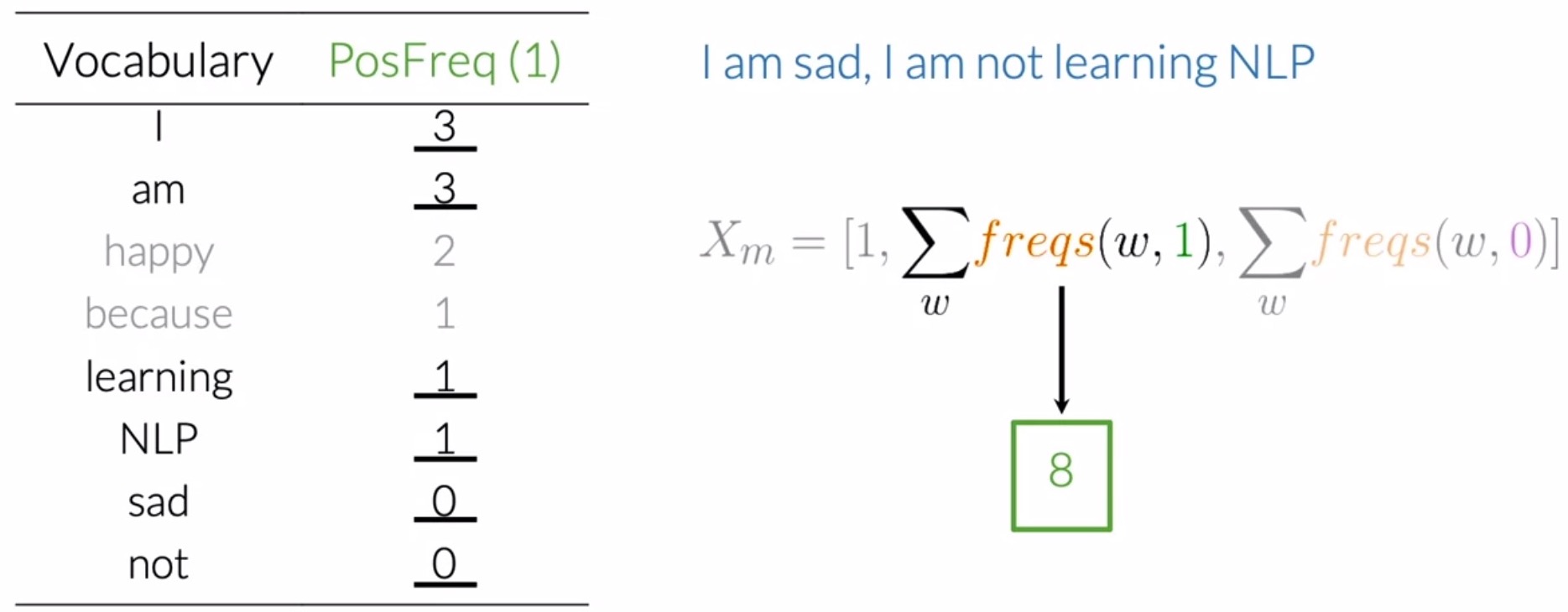
- For instance, looking at the frequencies for the positive class (which is the second feature being sought above) for the tweet shown below, the only words from the vocabulary that don’t appear on these tweets are happy and because. Summing up the frequencies for all the other words (underlined in the figure below), you’ll get a value equal to 8.
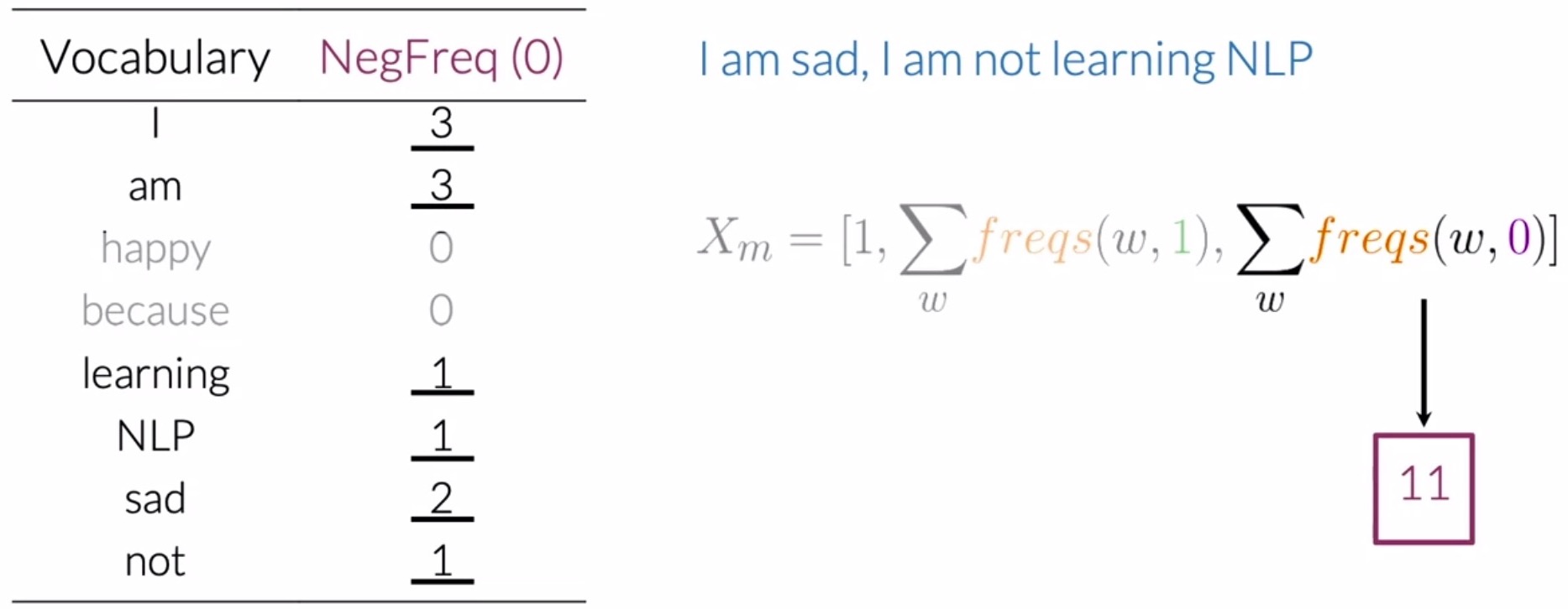
- Next, looking at the frequencies for the negative class (which is the third feature being sought above) for the same tweet, you need to sum the negative frequencies of the words from the vocabulary that appear on the tweet. For this example, you should get 11 after summing up the underlined frequencies.
- So, for our given example above, this representation would be equal to the vector \([1, 8, 11]\), which is a vector of dimension 3, as shown below.
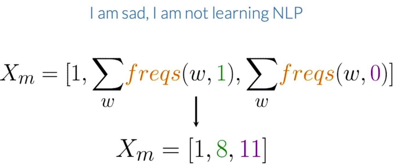
- In summary, you’re using the frequency dictionary to extract features for the positive/negative class for sentiment analysis, to represent a tweet using a vector of dimension 3.
[bias = 1, sum of the positive frequencies for every unique word on tweet, sum of the negative frequencies for every unique word on tweet]
- Next, let’s learn to pre-process your tweets and use these preprocessed words in place of words in your vocabulary.
Preprocessing
- Preprocessing is the idea of distilling a dataset so that it only contains essential information for the downstream task. A byproduct of preprocessing is that it helps in reducing the size of our vocabulary, which in turns saves training and test time as discussed in the section on sparse representations.
- There are four major preprocessing concepts in NLP:
- Tokenization
- Removing stop words and punctuation
- Stemming
- Lower-casing
Tokenization
- To tokenize a string means to split the strings into individual words without blanks or tabs.
Stop words and punctuation marks
- Consider the below tweet. First, remove all the words that don’t add significant meaning to the tweets, i.e., stop words and punctuation marks. In practice, you would compare your tweet against two lists, one with the stop words and another with punctuation.
- Note that these lists are usually much larger, but for the purpose of this example, we’ve kept them short and simple.
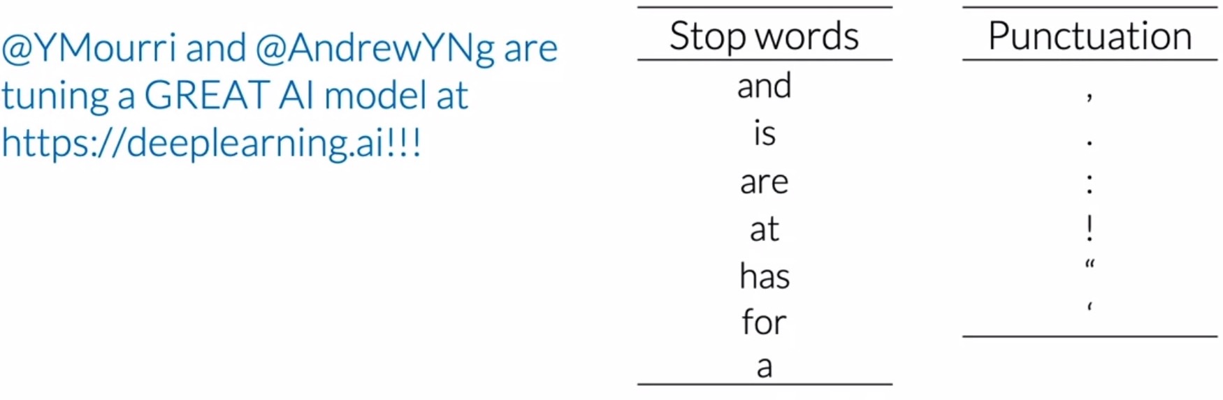
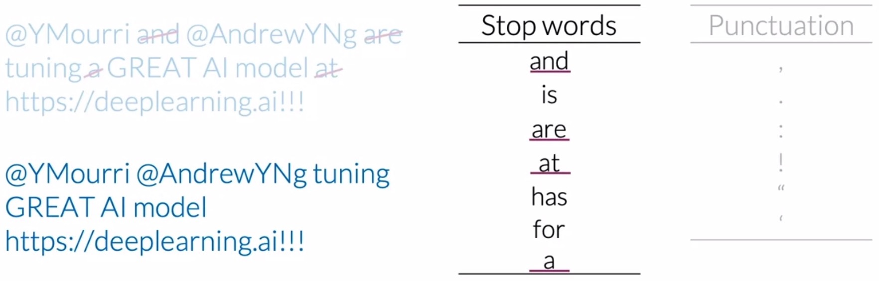
- Every word from the tweet that appears on the list of stop words should be eliminated. So you would have to eliminate the word and, the word are, the word a, and the word at.
- Show below in the figure is the tweet with the stop words trimmed out. Note that the overall meaning of the sentence can still be inferred without much effort.
-
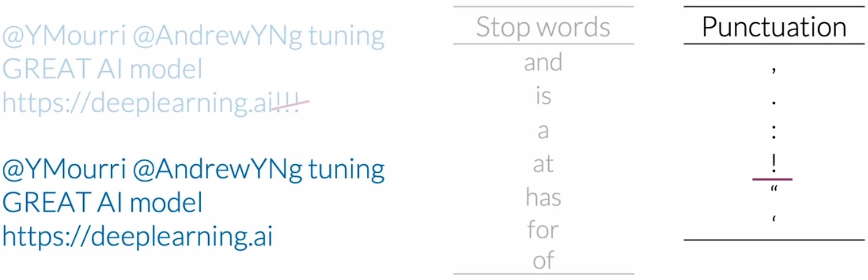
Now, let’s eliminate punctuation marks, which in the above e.g., are only exclamation marks.
-
The preprocessed tweet without stop words and punctuation is shown below. However, note that in some contexts eliminating punctuation is not desired and in fact, adds important information to your specific task. You might thus need to customize the list of stop words depending on your task at hand.
- Note that certain groupings like
:)and...should be retained when dealing with tweets because they are used to express emotions.
Task-dependent stop words
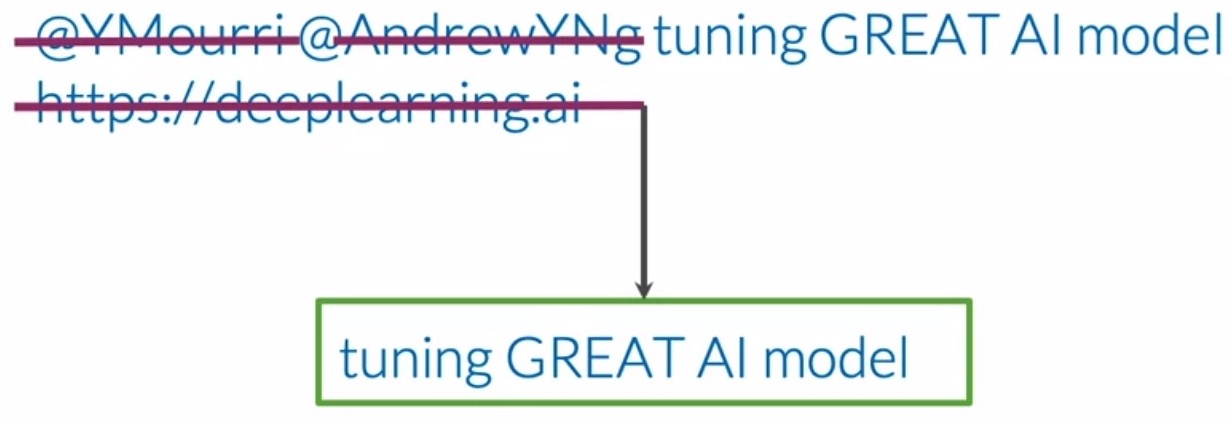
- Tweets often have handles, URLs, hashtags, stock market tickers and retweet marks, which generally don’t add any value to our particular task of sentiment analysis. These can also be treated as another set of “stop words” for the purposes of preprocessing for the specific task at hand.
- Upon eliminating the two handles and URL in the tweet, the resulting tweets only contains important information related to its sentiment. “Tuning GREAT AI model” is clearly a positive tweet and a sufficiently good model should be able to classify it.
Stemming
- In NLP, stemming is simply transforming any word to its most general form or base stem, which can be defined as a set of characters that are used to construct the word and its derivatives.
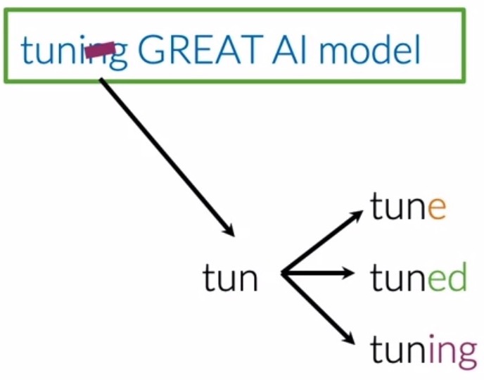
- Let’s take the first word tuning as an example (shown below). It’s stem is tun, because:
- Adding the letter e, makes it forms the word tune.
- Adding the suffix ed, forms the word tuned.
- Adding the suffix ing, it forms the word tuning.
- After you perform stemming on your corpus, the word tune, tuned, and tuning will all be reduced to the stem tun. This leads to your vocabulary being significantly reduced when you perform stemming for every word in the corpus, since you are effectively eliminating all variations of a particular word, but one.
- Some more examples:
- learn, learning, learned and learnt stem from their common root: learn.
- motivation, motivated, and motivate originate from their common stem: motiv.
- However, in some cases, stemming process produces words that are not correct spellings of the root word. For e.g., we can look at the set of words that comprises the different forms of happy: happy, happiness and happier. We can see that the prefix happi the most common stem throughout the entire set of related words. Note that we cannot choose happ because it is the stem of unrelated words like happen.
- The Porter Stemming Algorithm is a common algorithm for carrying out stemming in popular NLP libraries like NLTK.
Lower-casing
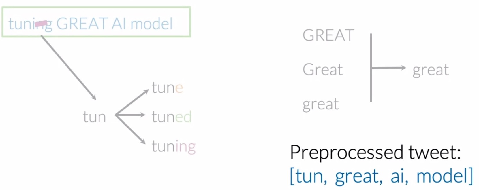
- To reduce your vocabulary even further without losing valuable information, you can lowercase all words in your tweet and then sift out the unique ones.
- So, in this case, the words GREAT, Great and great all would be treated as the same exact word. Thus, the final preprocessed-tweet as a list of words, becomes:
Generating the features matrix
- The next step is to create a matrix \(X\) that houses the features of your training examples \(m\). To generate \(X\):
- Step 1: Preprocess your tweet to get a list of words that contain that convey relevant information for the downstream task (in this case, sentiment classification), using the concepts discussed in the prior section on preprocessing.
- Step 2: Based on the output from step 1, you can obtain the positive/negative frequencies of each unique word in the sample using the frequency dictionary.
- Step 3: Obtain a vector with a bias unit and two additional features that store the summation of the positive and negative frequencies of each unique word in the sample.
- The figure below illustrates the above process of generating \(X\) from your input \((Input \rightarrow X)\):
- Practically, you would have to perform this process on a set of \(m\) raw tweets, where \(m\) is your dataset size. You would preprocess them one by one to get a list of essential words, one list per tweet. Next, you would be able to extract positive/negative features using a frequencies dictionary mapping.
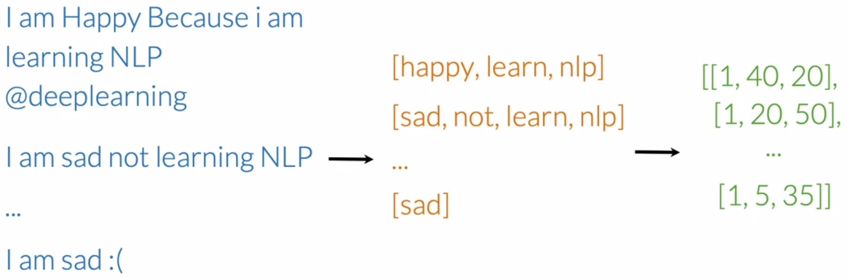
- This yields a matrix \(X\) with \(m\) rows and 3 columns, where every row contains the features for a corresponding tweet sample (note that the first row of \(X\) is highlighted in the below figure, which corresponds to the first sample, denoted by \(X^{(1)}\)).
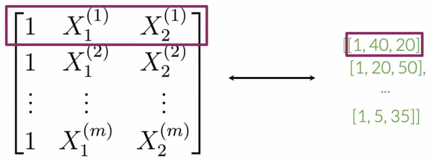
- The concept we’ve illustrated here involves packing features from multiple training examples together and operating on them simultaneously, rather than one-by-one. This is the concept of “vectorization” (more on this on the section on vectorization).
Putting it all together in code
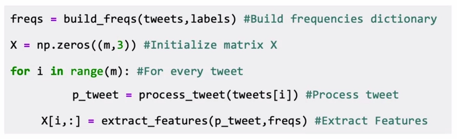
- In code, the overall process of (i) preprocessing, (ii) generating individual features for each tweet sample and, (iii) building matrix \(X\), involves the following steps:
- Step 1:
builds_freqs()builds the positive/negative frequencies dictionary. - Step 2:
np.zeros()initializes feature matrix \(X\) with zeros. Set the number of rows as number of tweets and the number of columns as 3 to accommodate 3 features per sample. - Step 3:
process_tweet()performs preprocessing on each tweet by (i) deleting stop words, punctuation, task-specific stop words (URLs, twitter handles etc.) and (ii) performing stemming and lower-casing. - Step 4:
extract_features()extracts features by summing up the positive and negative frequencies of each unique word within each tweet. The feature set for each tweet sample, comprising of[1, sum of the positive frequencies for every unique word on tweet, sum of the negative frequencies for every unique word on tweet]is assigned to the \(i^{th}\) row (corresponding to the \(i^{th}\) tweet sample) within \(X\).
- Step 1:
Logistic regression as a classifier
- The extracted feature matrix \(X\) generated in the above step is fed into a binary classifier since our task involves predicting a 1 or 0 label corresponding to positive and negative sentiment respectively. In this particular instance, we’re using the logistic regression classifier for binary classification.
Background
- Logistic regression is a supervised learning algorithm, which implies that the expected outputs, i.e., ground-truth labels \(Y\) corresponding to each training sample in \(X\) are available during training.
- Logistic regression takes a regular linear regression \(z\) and applies a hypothesis function on top of it (more on the hypothesis function in the section on sigmoid function).
- Formally:
- Note that in some literature, \(z\) is referred to as the ‘logit’, which essentially serves as the input to the hypothesis function.
- Note that the parameter vector \(\theta\) is also referred to simply, as “weights”. In some contexts, weights are referred to using a \(w\) vector or \(W\) matrix.
Sigmoid function
- In the figure below from the section on supervised machine learning, the transformation function \(F(\cdot)\) that operates on parameters \(\theta\) and the feature vector \(X^{(i)}\) to yield the output \(\hat{Y}\), is also known as the hypothesis function.
- Specifically, \(h(x^{(i)}; \theta)\) denotes the hypothesis function, where \(i\) is used to denote the \(i^{th}\) observation or data point. In the context of tweets, it’s the \(i^{th}\) tweet in the dataset.
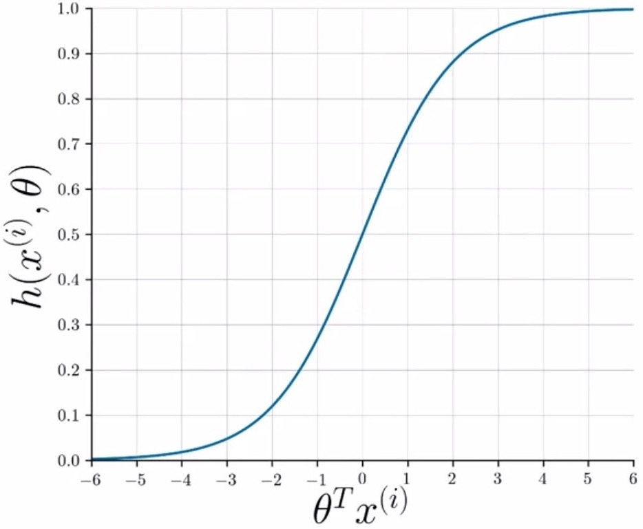
- In logistic regression, the sigmoid function serves as the hypothesis function. Logistic regression makes use of the sigmoid function which squeezes/collapses/transforms the input into an output range of \([0, 1]\), and can interpreted as a probability measure. Note that outside of the context of logistic regression, specifically in neural networks, the sigmoid function serves as a non-linearity and is denoted by \(\sigma(\cdot)\).
- Formally:
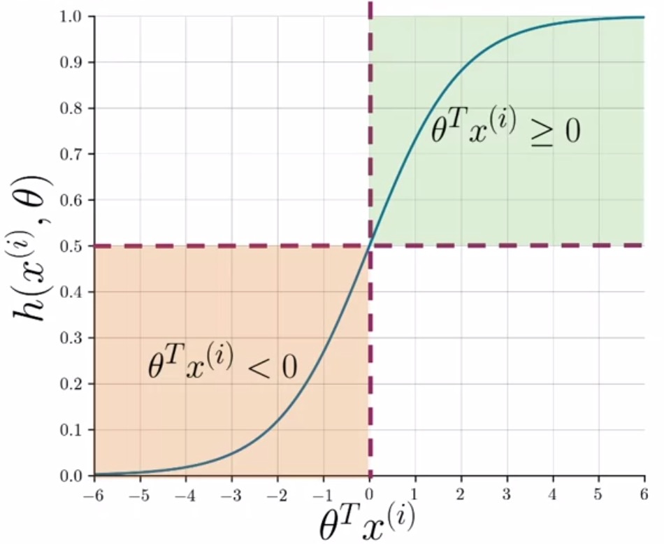
- Visually, the sigmoid function is shown below – it approaches 0 as the dot product of \(\theta^T x^{(i)}\) approaches \(- \infty\) and 1 as the dot product approaches \(\infty\).
Classification using logistic regression
- For classification, a threshold is needed. Usually, it is set to be \(0.5\) and this value corresponds to a dot product \(\theta^T x^{(i)}\) equal to 0.
- As shown below, whenever the dot product is \(\geq\) 0, the prediction is positive, and whenever the dot product is \(<\) 0, the prediction is negative.
- Formally,
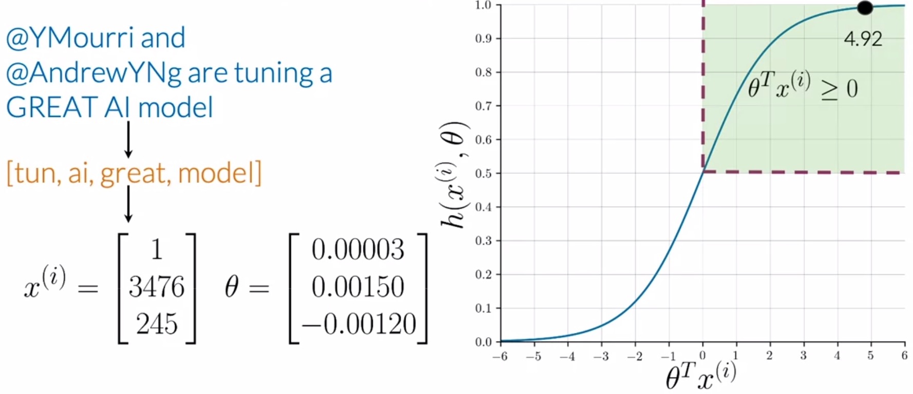
- Consider the example shown below in the figure.
- After preprocessing the tweet and fetching a list of essential words (shown in orange), you can extract features given a frequencies dictionary and arrive at a vector \(x^{(i)}\). This feature vector for the \(i^{th}\) sample has a bias unit as the first feature, and two additional features that are the sum of positive and negative frequencies of the unique words in your processed tweets.
- Assuming that you already have an optimum set of parameters \(\theta\), your sigmoid function outputs \(4.92\) in this case, which leads to the prediction of a positive sentiment.
Computing gradients
- Since computing gradients are the biggest component of the overall training process, we detail the process here.
- To update your weight vector \(\theta\), you will apply gradient descent to iteratively improve your model’s predictions.
-
The gradient of the cost function \(J(\theta)\) with respect to one of the weights \(\theta_j\) is denoted by \(\frac{\partial J(\theta)}{\partial \theta_j}\) (or equivalently, \(\nabla_{\theta_j}J(\theta)\)) as below. “Partial Gradient of the Cost Function for Logistic Regression” delves into the derivation of this equation.
\[\frac{\partial J(\theta)}{\partial \theta_j} = \nabla_{\theta_j}J(\theta) = \frac{1}{m} \sum\limits_{i = 1}^m (\hat{y}^{(i)}−y^{(i)})x_j\]- where,
- \(i\) is the index across all \(m\) training examples.
- \(j\) is the index of the weight \(\theta_j\), so \(x_j\) is the feature associated with weight \(\theta_j\).
- \(\hat{y}^{(i)}\) (or equivalently, \(h(X^{(i)}; \theta))\) is the model’s prediction for the \({i}^{th}\) sample.
- where,
Update rule
-
To update the weight \(\theta_j\), we adjust it by subtracting a fraction of the gradient determined by \(\alpha\):
\[\theta_j := \theta_j − \alpha \times \nabla_{\theta_j}J(\theta)\]- where \(:=\) denotes a paramater/variable update.
- Note that the above weight-update equation is called as the update rule in some literature.
- The learning rate \(\alpha\), or the step size, is a value that helps us choose to control how big of a step a single update during our training process would involve.
Training logistic regression
- In the section on classification using logistic regression, we made an assumption that an optimum set of parameters \(\theta\) were available when inferring our prediction. In this section, we do away with this assumption and generate the optimum set of parameters \(\theta\) by putting together the following ideas we talked about in the prior sections:
- To train your logistic regression classifier, i.e., learn \(\theta\) from scratch, iterate until you find the set of parameters \(\theta\) that minimize your cost function until convergence.
Convergence is defined as the point during training where the overlap between your prediction and ground-truth distributions is at its peak.
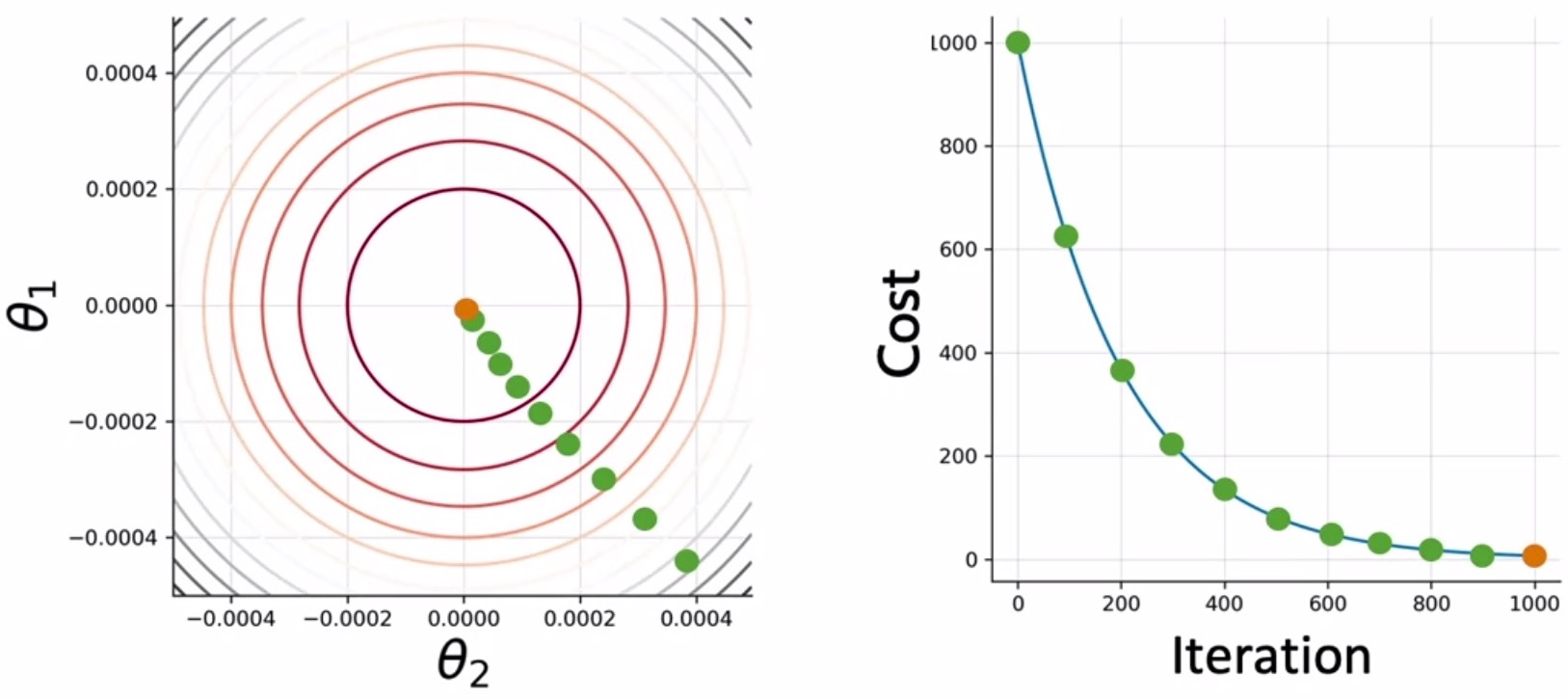
- To ease the process of visualization, assume that the loss only depends on the parameters \(\theta_1\) and \(\theta_2\), the cost function can be represented as a 2D contour plot, as shown on the left side of the figure. On the right, you can see the evolution of the cost function as we iterate.
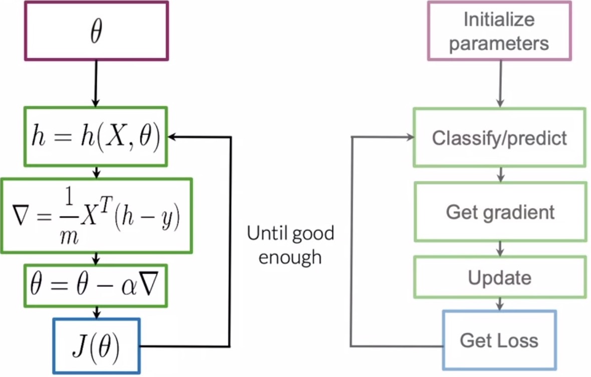
- The following steps outline the process of training:
- Initialize parameters: Initialize the parameter vector \(\theta\) randomly or with zeros.
- Calculate logits: The logits \(z\) are calculated using the dot product of the feature vector \(x\) with the weight vector \(\theta\), i.e., \(z=\theta^T x\).
- Apply a hypothesis function: Use the sigmoid function \(h(\cdot)\) element-wise to transform each feature of each sample.
- Generate the final prediction: Generate the final prediction \(\hat{y}\) by comparing each element obtained at the output of the prior step with a static threshold, of say \(0.5\) and inferring a 1 if the element \(\geq\) 0, else 0.
- Compute the cost function: Compute your cost function \(J(\theta)\) to determine how far we are from our expected output (note that \(J(\theta)\) can be viewed as a measure of our unhappiness quotient towards the model’s accuracy).
- The cost function basically tells us if we need more iterations before we converge to a minimized loss (or can be bounded by a “maximum” cap on the number of iterations). Typically, after several iterations, you reach your minima where your cost is at its minimum and you would end your training here.
- Calculate gradients: Calculate the gradients of your cost function w.r.t. each parameter in the parameter vector \(\theta\).
- Apply update rule: Update your parameter vector \(\theta\) in the direction of the gradient of your cost function using your update rule.
- After a set of iterations, you traverse along the loss curve (shown by the green dots in the figure above) and get closer to your minima where you would end your training here when you converge (shown by the orange dot).
This algorithm is known as gradient descent, where the name is derived from the fact that we’re using gradients to route over the channels in the parameter-space that lead to the loss being minimized (until convergence).
- The figure below illustrates the above process of training via gradient descent:
- Models are typically trained for several epochs, where each epoch is a loop over the entire training set. In other words, an epoch has elapsed when your model has seen every example in the training dataset once.
Vectorization
- Next, let’s explore how we can optimize the process of gradient descent and make it efficient by dealing with all of our training examples in one shot, rather than attending to each sample one-by-one. To this end, a discussion on the dimension property of matrices and the concept of dimension balancing is worthwhile.
Dimension property of matrices
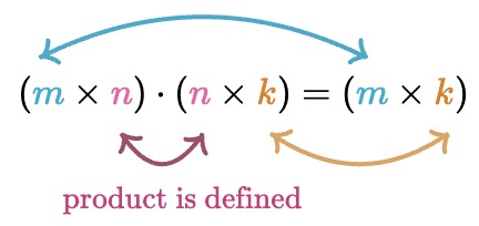
- During matrix multiplication, checking for the appropriate matrix dimensions is important to ensure your matrices satisfy the dimension property (illustrated in the figure below), which states that:
- The product of two matrices is defined if and only if the number of columns in the first matrix is equal to the number of rows in the second matrix.
- If the product is defined, the resulting matrix will have the same number of rows as the first matrix and the same number of columns as the second matrix.
Dimension balancing
- Dimension balancing can be best explained using some practical examples.
- Consider the case of multiplying two vectors of the same type, i.e., row vectors or column vectors. Let’s assume that we have two column vectors \(a\) and \(b\) of size \((m, 1)\), we need to transpose the vector to the left to be able to obtain the inner-dot product of the vectors (which is a scalar). The case of two row vectors can be handled similarly. Formally:
- Key takeaways:
- In the above example, the center dimension \(m\) needs to overlap for both vectors for multiplication to be defined, which follows from the dimension property of matrices that we reviewed earlier. In other words, the vectors need to be similar-sized for their dot product to be defined.
- Note that if the vectors are of different types, i.e., say, one is a row vector while the other is a column vector, the transposing operation (which is part of dimension balancing) is not needed. This case can be decomposed into two sub-cases:
- Dot-product of a row vector and a column vector: \((1, m) \cdot (m, 1) = (1, 1)\)
- In this case, again, the center dimension needs to overlap (i.e., the vectors need to be similar-sized) for the dot-product to be defined.
- Multiplication of a column vector and a row vector: \((m, 1) \cdot (1, n) = (m, n)\)
- In this case, given the two entities undergoing the multiplication operation are vectors, the center dimension (which is 1) automatically overlaps. In this case, the vectors do not need to be similar-sized. Note that this yields a matrix and not a scalar, and thus represents the multiplication of two vectors and not their dot-product.
- Dot-product of a row vector and a column vector: \((1, m) \cdot (m, 1) = (1, 1)\)
- As another example, let’s consider the case of multiplying a vector and a matrix. Assume that we have a matrix \(A\) of size \((m, n)\) and vector \({b}\) of size \((m, 1)\). In this case, we need to transpose \(X\) and place it on the left in order to satisfy the dimension property above, and yield a vector (of the same “row/column”-vector type as the input vector) at the output. Formally:
Implementing vectorization
- We saw a preview of vectorization in the section on generating the features matrix. In this section, we offer a deeper treatment on the topic.
- Vectorization is the process of converting an algorithm from operating on a single value at a time to operating on a set of values (vectors/arrays) simultaneously.
- Under the hood, modern CPUs provide direct support for vector operations where a single instruction is applied to multiple data (SIMD).
- For e.g., a CPU with a \(512\) bit register could hold 16 \(32\)-bit single precision doubles and do a single calculation \(16x\) faster than executing a single instruction at a time. Combining this with threading and multi-core CPUs leads to orders of magnitude performance gains.
- Overall, the process we laid out in the section on training logistic regression remains similar, with small changes at the relevant steps to accommodate operations on multiple training examples (in our particular case, the entire training dataset of \(m\) examples), rather than attending to individual examples one-by-one.
- To vectorize gradient descent, for each iteration of your training loop, you’ll calculate the cost function \(J(\theta)\) using all \(m\) training examples simultaneously (assuming we’re using “batch gradient descent” here, other alternatives exist that let you operate on a mini-batch of examples at a time).
- To do so, we’ll need to:
- Initialize parameters: Initialize the parameter vector \(\theta\) randomly or with zeros.
- Vectorize ground-truth labels: the ground-truth labels \(y\) by stacking them into a column vector.
- Matricize training dataset: Assemble all the samples in our training dataset as a matrix \(X\), with the \(i^{th}\) sample at the \(i^{th}\) row of the matrix.
- Formally:
- Calculate logits: The logits \(z\) are calculated using the dot product of the feature matrix \(X\) with the weight vector \(\theta\), i.e., \(z=X\theta\)
- \(X\) has dimensions \((m, n+1)\)
- \(\theta\) has dimensions \((n+1, 1)\), where \(n\) is the number of features, and the additional element is for the bias term \(\theta_{0}\) (note that the corresponding feature value \(x_{0}\) is 1).
- \(z\) has dimensions \((m, 1)\) because \((m, n+1) \cdot (n+1, 1) = (m, 1)\) owing to the dimension property of matrices.
- Apply a hypothesis function: Next, we apply the sigmoid/hypothesis function \(h(\cdot)\) to each logit \(z\), i.e., \(h(z)=\operatorname{sigmoid}(z)\).
- \(h(X; \theta)\) has the same dimensions as \(z\), i.e., \((m, 1)\), because the sigmoid operation \(h(\cdot)\) is applied element-wise.
- Generate the final prediction: Lastly, the output prediction \(\hat{y}\) is obtained by comparing each element of the resultant vector \(h(X; \theta)\), with a static threshold, of say \(0.5\) and inferring a 1 if the element \(\geq\) 0, else 0.
- \(\hat{y}\) has the same dimensions as \(h(X; \theta)\) (or \(z\)) because the thresholding operation is applied element-wise.
- The output prediction \(\hat{y}\) can be formally visualized below:
- Compute the cost function: The cost function \(J(\theta)\) is calculated by taking the following vector dot products: (i) \(y\) and \(log(\hat{y})\) and, (ii) \({1}-{y}\) and \(log({1}-{\hat{y}})\), followed by summing them together and averaging this result over \(m\) training examples.
- Since both \(y\) and \(\hat{y}\) are column vectors of dimensions \((m, 1)\), we need to dimension balance and transpose the vector to the left, so that the multiplication of a row vector with column vector yields the desired dot product, as shown in the equation below:
- Instead of updating a single weight \(\theta_{i}\) at a time, we can also vectorize the process of updating parameters by updating all the weights in the column vector \(\theta\). We fetch the update rule from the section on update rule, and vectorize it by:
- Ignoring the \(j\) index corresponding to the \(j^{th}\) weight in the parameter vector \(\theta\), signifying that we’re using the entire parameter vector \(\theta\) for computation rather than an individual element in the vector.
- Calculate gradients: To obtain the vectorized gradient of the loss function partial derivative, we use the derivation in “Partial Gradient of the Cost Function for Logistic Regression”, and vectorize it by:
- Ignoring the \(i\) and \(j\) indices corresponding to the \(i^{th}\) training example and \(j^{th}\) weight respectively (and thus letting go of the summation in the process).
- Considering the features matrix \(X\) instead of the feature vector \(x\).
- Because the dimensions of \(X\) are \((m, n)\) and both \({\hat{y}}\) and \({y}\) are \((m, 1)\), we need to transpose \(X\) and place it on the left in order to perform matrix multiplication (again, we’re carrying out dimension balancing).
- Apply update rule: Substituting the above equation in the vectorized update rule yields the \((n+1, 1)\)-dimensioned \(\theta\) we’re seeking:
- Rather than attending to samples one by one in a loop, vectorization is the preferred implementation route since it drastically speeds up the training/inference process by several orders of magnitude, especially on modern CPUs and GPUs that offer enhanced parallelism. Read more on SIMD/AVX instructions here.
- Vectorization as a concept can extend to any kind of dataset. Similar to how we vectorized the entire set of training samples, we can carry out vectorization of the testing dataset as well, rather than feeding individual examples to the model at test time.
Testing logistic regression
- To evaluate the generalization ability of your classifier and thus, test your model, generate predictions on unseen data (data that the model has not come across during training) and check how well it fares.
- Pre-requisites:
- \(X_{val}\) and \(Y_{val}\): samples and their corresponding labels that were set aside during training (i.e., the validation set).
- \(\theta\): the set of optimum parameters that lead to a minimized loss, obtained as part of training.
- Armed with \((X_{val}: Y_{val}) \) and \(\theta\), we carry out the below steps to compute the accuracy of our model:
- Apply the sigmoid function:
- Compute the sigmoid function \(h(\cdot)\) for \(X_{val}\) with parameter vector \(\theta\).
- This is formally denoted as \(h(X_{val}; \theta)\), and referred to as \(h\) being a function of \(X_{val}\) parameterized by \(\theta\).
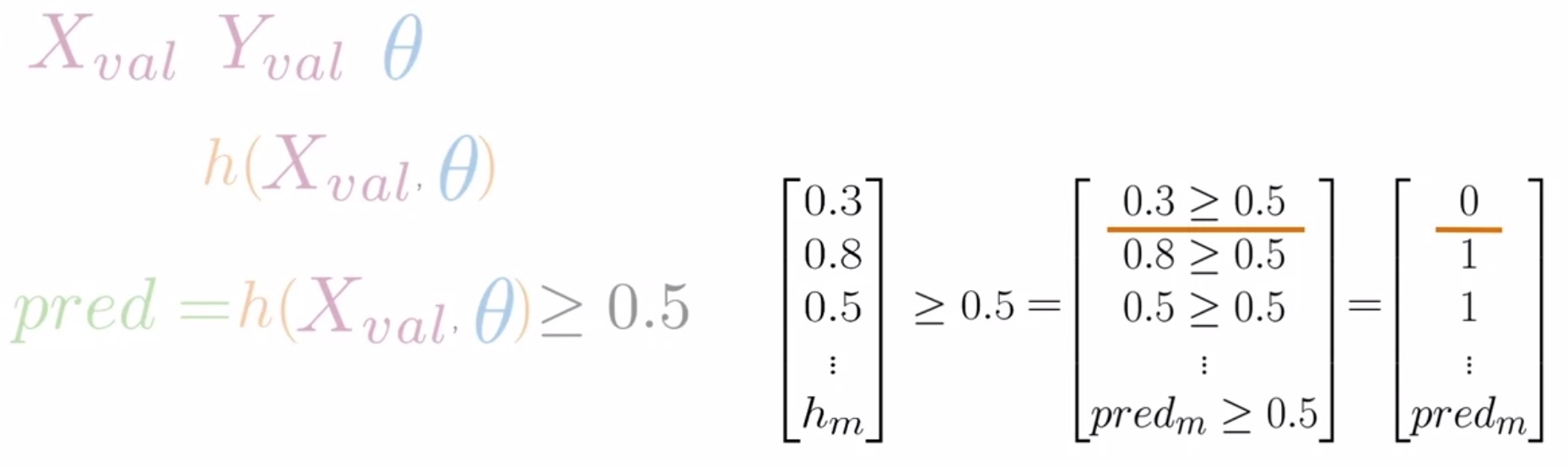
- Inferring your predictions using a static threshold:
- Evaluate if each value of \(h(X_{val}; \theta)\) is \(\geq\) to a threshold value, often set to \(0.5\).
- For e.g., let’s assume \(h(X_{val}; \theta)\) is \([0.3, 0.8, 0.5]\), where the \(i^{th}\) value corresponds to the \(i^{th}\) sample from your validation set.
- Next, you’re going to assert if each of the components of \(h(X_{val}; \theta)\) is \(\geq\) to \(0.5\).
- Is \(0.3\) \(\geq\) \(0.5\)\(?\) No. So our first prediction is equal to 0 (shown in the figure below with the orange underline).
- Is \(0.8\) \(\geq\) \(0.5\)\(?\) Yes. So our prediction for the second example is 1.
- Is \(0.5\) \(\geq\) \(0.5\)\(?\) Yes. So our third prediction is equal to 1, and so on.
- At the end, you will have a vector populated with zeros and ones indicating predicted negative and positive examples, respectively.
- Compute the overlap between predictions and the ground-truth:
- Compare the predictions with the ground-truth from your validation data. Generate booleans of 1 and 0 corresponding to whether your predictions are match your ground-truth or not, respectively.
- For e.g., if your prediction was correct, say in this case where both your prediction and your label are equal to 0, your vector will have a value equal to 1 in the first position (shown on the right-hand-side in the below figure with a green underline).
- Conversely, if your second prediction wasn’t correct because your prediction and label disagree, your vector will have a value of 0 in the second position and so forth.
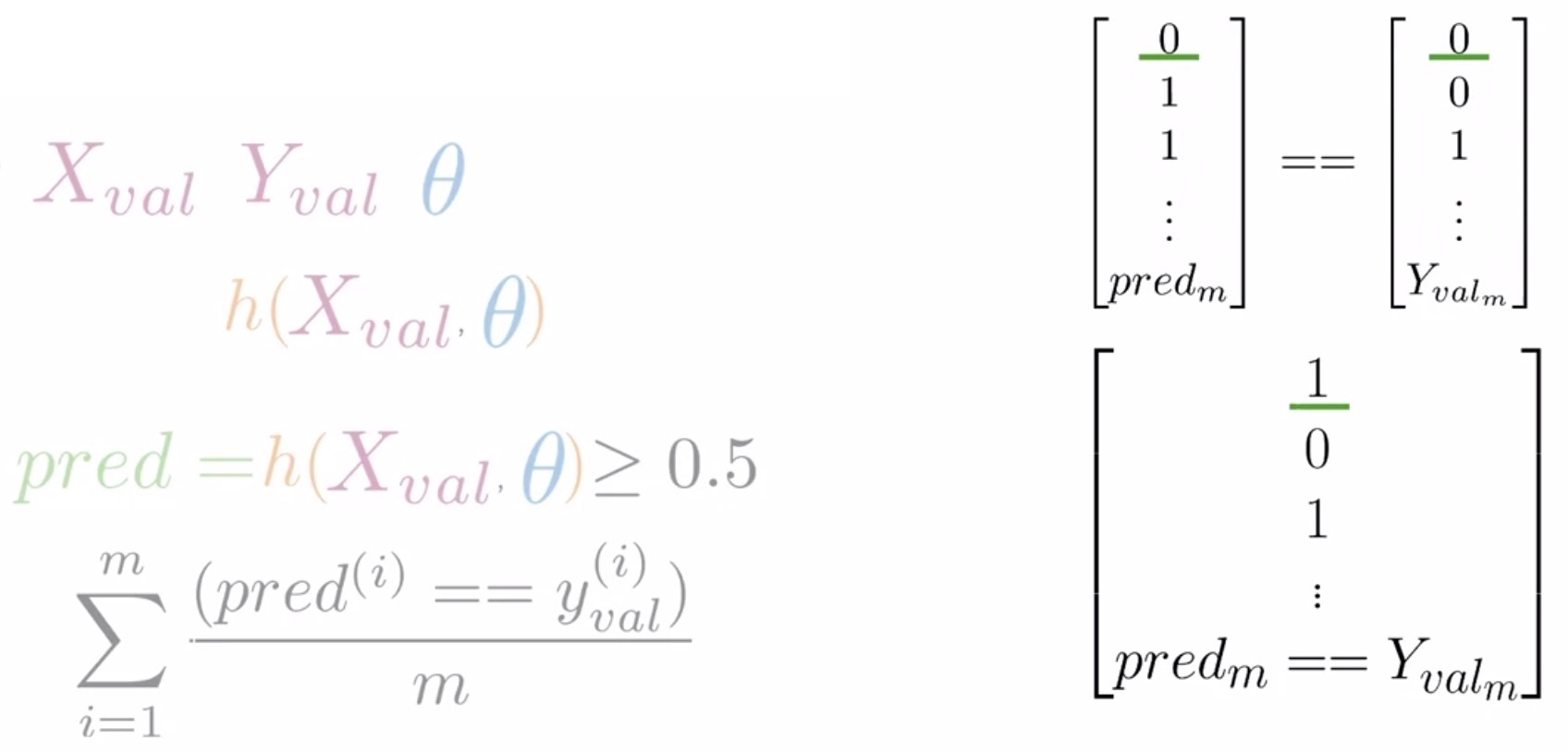
- Compute the model’s accuracy on the validation set:
- To obtain the accuracy of your model:
- Calculate the number of times that your predictions were correct by summing up the vector of the comparisons (since each correct prediction is essentially represented as a 1 in this vector).
- Divide this number by the total number of samples/observations in your validation set, say \(m\), as shown on the left-hand-side in the above figure.
- This metric gives an estimate of how your logistic regression model will fare on unseen data.
- Thus, if your accuracy is equal to \(0.5\), it means that \(50\%\) of the time, your model is expected to do the right thing.
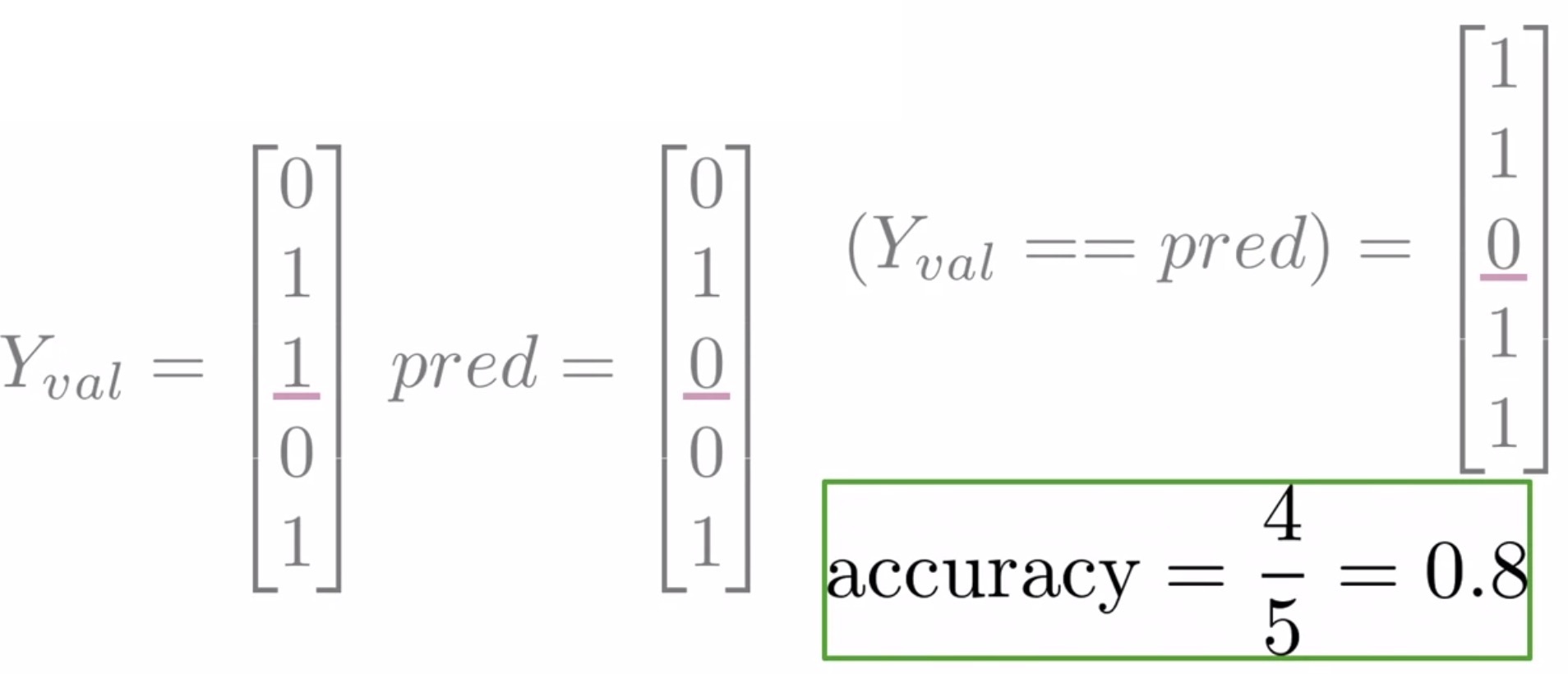
- For e.g., assume your \(Y_{val}\) and prediction vectors for 5 observations are as in the figure below.
- Upon comparing each of their values, you’ll have the following vector with a single 0 in the third position where the prediction and the label disagree.
- Next, you sum the number of times that your predictions were right and divide that number by the total number of observations in your validation set. This yields an accuracy of \(80\%\).
- To obtain the accuracy of your model:
Cost function intuition
- Let’s dissect the cost function for logistic regression to build the intuition behind it.
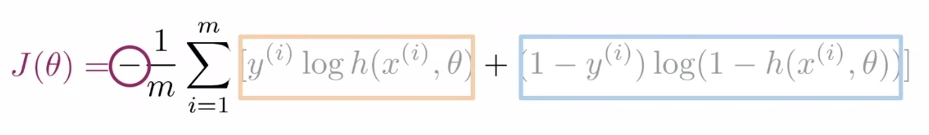
- The cost function used for logistic regression is the average of the log loss across all training examples. Formally:
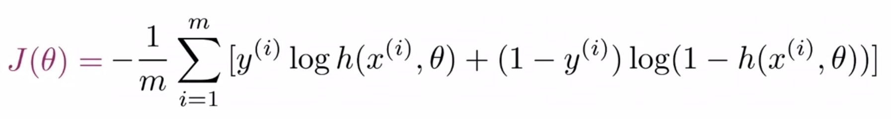
- where,
- \(m\) is the number of training examples.
- \(y^{(i)}\) is the actual/ground-truth label of the \(i^{th}\) training example.
- \(h(z(\theta)^{(i)})\) (or equivalently, \(h(h(x^{(i)}); \theta)\), or simply, \(\hat{y}^{(i)}\)) is the model’s prediction for the \(i^{th}\) training example.
- Let’s break it down into its components. Look at the left-hand side of the equation where you find a sum over the variable \(m\), which is the number of samples in your training set. This indicates that you’re going to sum over the cost of each training example. Also, out front, the \(\frac{-1}{m}\), indicates that when combined with the sum, this would lead to an averaging operation across all training examples.
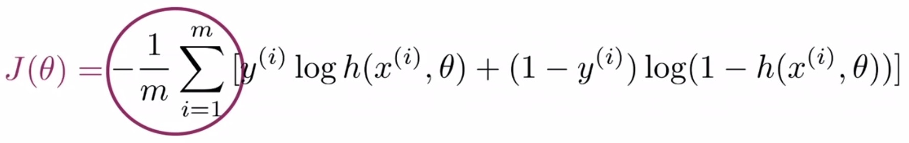
- Inside the square brackets, the equation has two terms that are added together, one on the left-hand side and the other on the right-hand side. To consider how each of these terms contribute to the cost function for each training example, let’s dive into each of them separately.
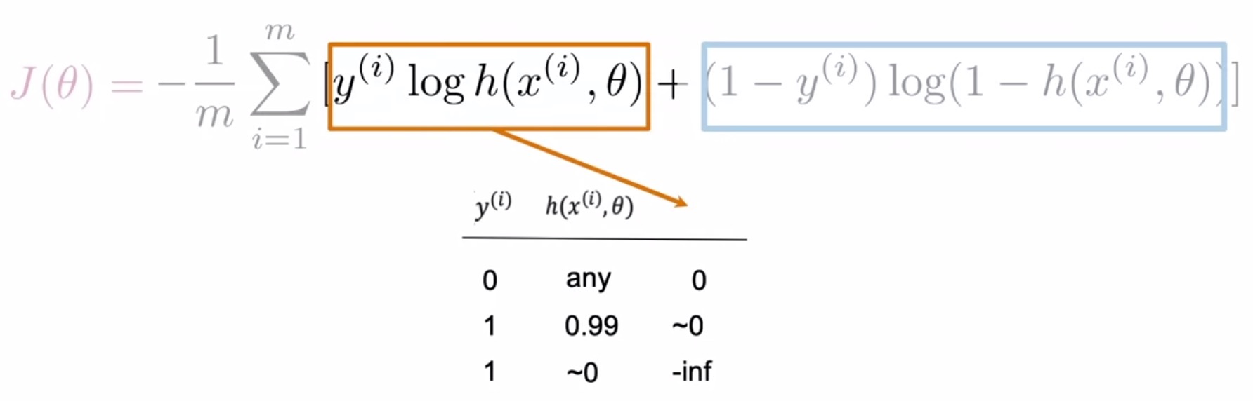
Left-hand side term
-
The term on the left is the product of \(y^{(i)}\), which is the label for each training example and the log of the prediction \(\log(h(x^{(i)}); \theta)\) (or equivalently, \(\log(\hat{y})\)), which is the logistic regression function being applied to each training example.
- Consider the case when your label is 0. In this case, the function \(h(\cdot)\) can return any value, and the entire term will be 0 because 0 times anything is just 0.
- Next, consider the case when your label is 1, and…
- If your prediction is close to (or “tends” to) 1, then the log of your prediction will tend to 0, because \(\log 1\) \(=\) 0, and thus the product will also tend to 0.
- If your prediction tends to 0, then this term blows up and approaches \(-\infty\), which is then multiplied by the overall factor of \(-1\) to convert it to \(+\infty\).
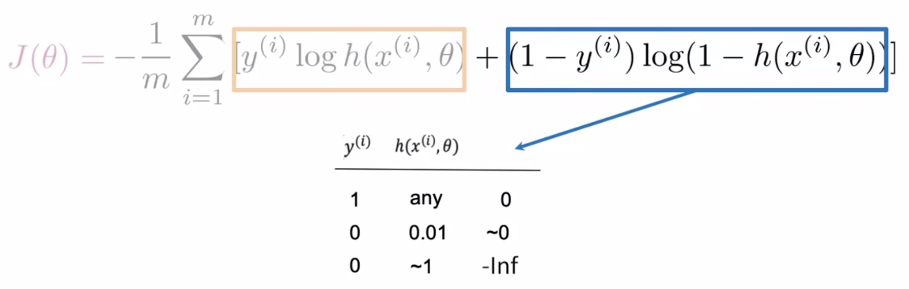
Right-hand side term
- Now, consider the term on the right-hand side of the cost function equation. In this case, if your label is 1, then the \(1 - y^{(i)}\) term goes to 0. And so any value returned by the logistic regression function will result in 0 for the entire term, because again, 0 times anything is just 0.
- If your label is 0, and…
- If your prediction tends to 0, then the products in this term will again tend to 0.
- If your prediction tends to 1, then the log term will blow up and the overall term approaches \(-\infty\), which is then multiplied by the overall factor of \(-1\) to convert it to \(+\infty\).
- The closer the model prediction gets to 1, the larger the loss. If the model’s prediction is \(0.9999\), the loss becomes \(−1 \times (1 − 0) \times \log(1 − 0.9999)\,\approx\,9.2\)
- Key takeaways:
- There is only one term in the cost function that is relevant when your label is 0 which is \(-\log(\hat{y}\)), and another that is relevant when the label is 1 which is \(-\log(1 - \hat{y}\)).
- Intuitively, when your prediction is close to the label value, the loss is small, and conversely when your label and prediction disagree, the overall cost goes up.
Overall Minus Sign
- In each of the left/right-hand side terms, you’re taking the log of a value between 0 and 1, which will always return a negative number. So, the minus sign out-front ensures that the overall cost will always be a positive number.
Geometric interpretation
- Let’s geometrically interpret what the cost function looks like for each of the labels, i.e., overall possible prediction values, 0 and 1.
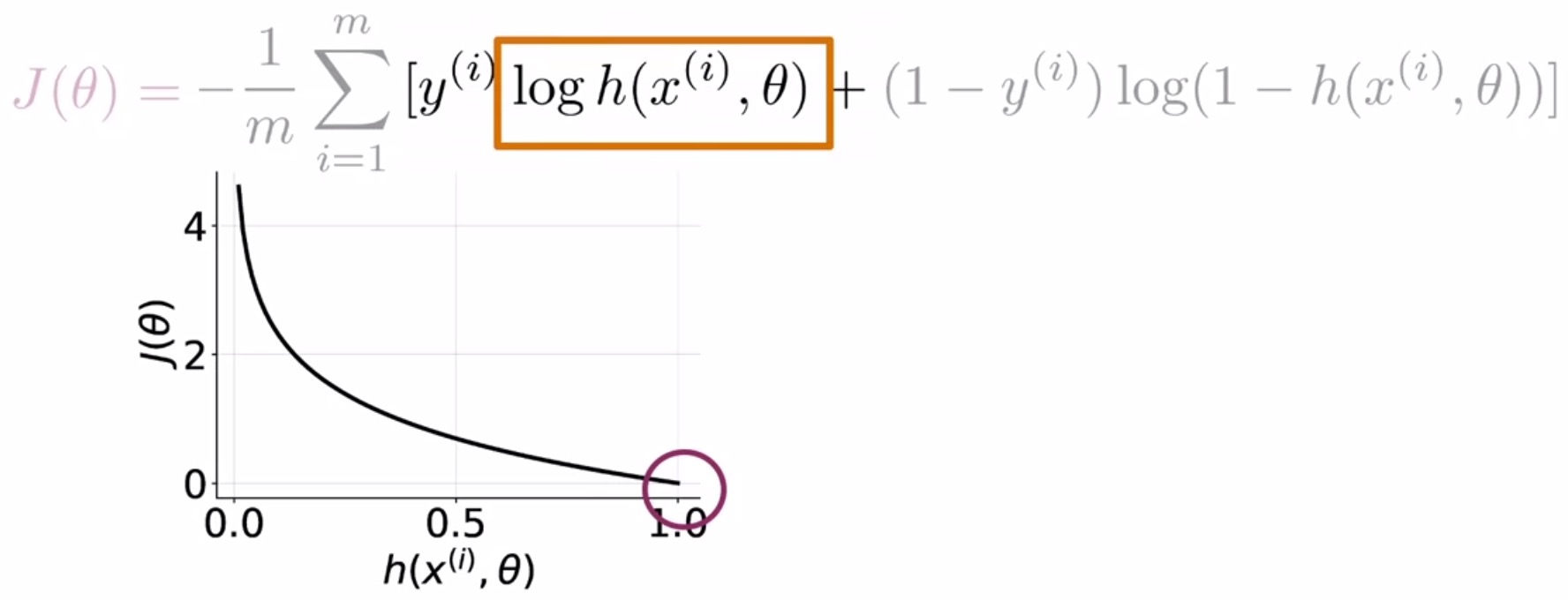
- First, we’re going to look at the loss when the label is 1.
- In the plot shown below, you have your prediction value on the horizontal axis and the cost associated with a single training example on the vertical axis.
- For \(y\,=\,1\), \(J(\theta)\) simplifies to just \(-\log(\hat{y})\).
- When the prediction tends to 1, the loss is close to 0, because your prediction agrees well with the label.
- When the prediction tends to 0, the loss approaches \(\infty\), because your prediction and the label disagree strongly.
- Formally,
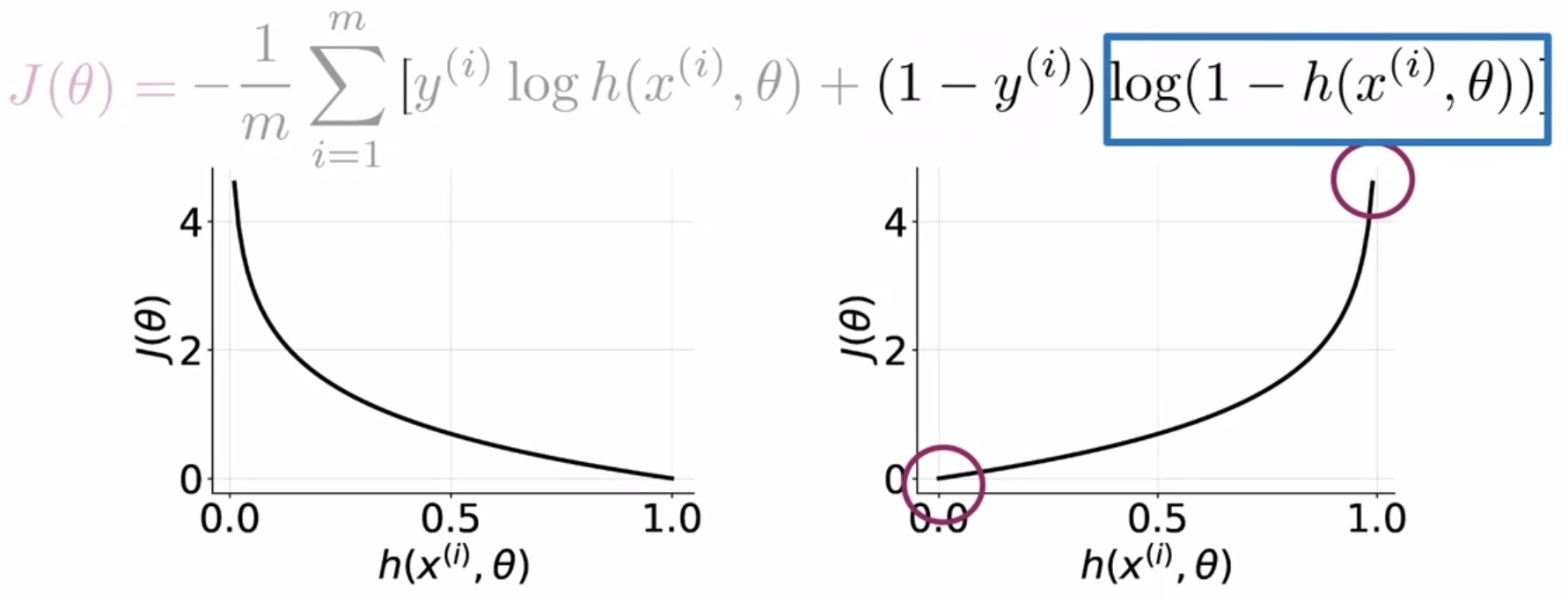
- Second, let’s explore the loss when the label is 0.
- In this case, the opposite is true when the label is 0, compared to the case above when the label is 1.
- For \(y\,=\,0\), \(J(\theta)\) reduces to just \(-\log(1 - \hat{y})\).
- When your prediction tends to 0, the loss is also close to 0.
- When your prediction tends to 1, the loss approaches \(\infty\).
- Formally,
Mathematical interpretation
- Now, let’s present a formal mathematical interpretation of what the cost function looks like for each of the labels.
- Consider the case when the label is 1. During optimization, since we’re trying to minimize the loss \(J(\theta)\), we want \(\hat{y}\) to be as large as possible, which in turn pushes \(\hat{y}\) towards 1 (which is the correct prediction).
- Next, consider the case when the label is 0. Again, during optimization, since we’re trying to minimize the loss \(J(\theta)\), we want \(1 - \hat{y}\) to be as large as possible, which in turn pushes \(\hat{y}\) to be as small as possible, towards 0 (again, which is the correct prediction).
Further reading
Here are some (optional) links you may find interesting for further reading:
- Partial Gradient of the Cost Function for Logistic Regression delves into the derivation of the partial derivative of the cost function for logistic regression.
- Dimension property to read more on matrix multiplication properties.
- Vectorization to understand the why and what of vectorization.
- Gradient Descent to explore the different types of gradient descent and their pros/cons.
Citation
If you found our work useful, please cite it as:
@article{Chadha2020DistilledSentimentAnalysisLogisticRegression,
  title   = {Sentiment Analysis using Logistic Regression},
  author  = {Chadha, Aman},
  journal = {Distilled Notes for the Natural Language Processing Specialization on Coursera (offered by deeplearning.ai)},
  year    = {2020},
  note    = {\url{https://aman.ai}}
}