and
#tags.txt B-PER B-LOC …
### Structure of the dataset

- Download the original version on the [Kaggle](https://www.kaggle.com/abhinavwalia95/entity-annotated-corpus/data) website.

- **Download the dataset:** `ner_dataset.csv` on [Kaggle](https://www.kaggle.com/abhinavwalia95/entity-annotated-corpus/data) and save it under the `nlp/data/kaggle` directory. Make sure you download the simple version `ner_dataset.csv` and NOT the full version `ner.csv`.

- **Build the dataset:** Run the following script:

```python
python build_kaggle_dataset.py
- It will extract the sentences and labels from the dataset, split it into train / test / dev and save it in a convenient format for our model. Here is the structure of the data
kaggle/
    train/
        sentences.txt
        labels.txt
    test/
        sentences.txt
        labels.txt
    dev/
        sentences.txt
        labels.txt
-
If this errors out, check that you downloaded the right file and saved it in the right directory. If you have issues with encoding, try running the script with Python 2.7.
-
Build the vocabulary: For both datasets,
data/smallanddata/kaggleyou need to build the vocabulary, with:
python build_vocab.py --data_dir data/small
- or:
python build_vocab.py --data_dir data/kaggle
Loading text data
- In NLP applications, a sentence is represented by the sequence of indices of the words in the sentence. For example if our vocabulary is
{'is':1, 'John':2, 'Where':3, '.':4, '?':5}then the sentence “Where is John ?” is represented as[3,1,2,5]. We read thewords.txtfile and populate our vocabulary:
vocab = {}
with open(words_path) as f:
    for i, l in enumerate(f.read().splitlines()):
        vocab[l] = i
-
In a similar way, we load a mapping
tag_mapfrom our labels fromtags.txtto indices. Doing so gives us indices for labels in the range \(\text{[0, 1, …, NUM_TAGS-1]}\). -
In addition to words read from English sentences,
words.txtcontains two special tokens: anUNKtoken to represent any word that is not present in the vocabulary, and aPADtoken that is used as a filler token at the end of a sentence when one batch has sentences of unequal lengths. -
We are now ready to load our data. We read the sentences in our dataset (either train, validation or test) and convert them to a sequence of indices by looking up the vocabulary:
train_sentences = []
train_labels = []

with open(train_sentences_file) as f:
    for sentence in f.read().splitlines():
        # replace each token by its index if it is in vocab
        # else use index of UNK
        s = [vocab[token] if token in self.vocab
            else vocab['UNK']
            for token in sentence.split(' ')]
        train_sentences.append(s)

with open(train_labels_file) as f:
    for sentence in f.read().splitlines():
        # replace each label by its index
        l = [tag_map[label] for label in sentence.split(' ')]
        train_labels.append(l)
- We can load the validation and test data in a similar fashion.
Preparing a Batch
- This is where it gets fun. When we sample a batch of sentences, not all the sentences usually have the same length. Let’s say we have a batch of sentences
batch_sentencesthat is a Python list of lists, with its correspondingbatch_tagswhich has a tag for each token inbatch_sentences. We convert them into a batch of PyTorch Variables as follows:
# compute length of longest sentence in batch
batch_max_len = max([len(s) for s in batch_sentences])

# prepare a numpy array with the data, initializing the data with 'PAD'
# and all labels with -1; initializing labels to -1 differentiates tokens
# with tags from 'PAD' tokens
batch_data = vocab['PAD']*np.ones((len(batch_sentences), batch_max_len))
batch_labels = -1*np.ones((len(batch_sentences), batch_max_len))

# copy the data to the numpy array
for j in range(len(batch_sentences)):
    cur_len = len(batch_sentences[j])
    batch_data[j][:cur_len] = batch_sentences[j]
    batch_labels[j][:cur_len] = batch_tags[j]

# since all data are indices, we convert them to torch LongTensors
batch_data, batch_labels = torch.LongTensor(batch_data), torch.LongTensor(batch_labels)

# convert Tensors to Variables
batch_data, batch_labels = Variable(batch_data), Variable(batch_labels)
- A lot of things happened in the above code. We first calculated the length of the longest sentence in the batch. We then initialized NumPy arrays of dimension
(num_sentences, batch_max_len)for the sentence and labels, and filled them in from the lists. -
Since the values are indices (and not floats), PyTorch’s Embedding layer expects inputs to be of the
Longtype. We hence convert them toLongTensor. -
After filling them in, we observe that the sentences that are shorter than the longest sentence in the batch have the special token
PADto fill in the remaining space. Moreover, thePADtokens, introduced as a result of packaging the sentences in a matrix, are assigned a label of-1. Doing so differentiates them from other tokens that have label indices in the range \(\text{[0, 1, …, NUM_TAGS-1]}\). This will be crucial when we calculate the loss for our model’s prediction, and we’ll come to that in a bit. - In our code, we package the above code in a custom
data_iteratorfunction. Hyperparameters are stored in a data structure called “params”. We can then use the generator as follows:
# train_data contains train_sentences and train_labels
# params contains batch_size
train_iterator = data_iterator(train_data, params, shuffle=True)

for _ in range(num_training_steps):
    batch_sentences, batch_labels = next(train_iterator)

    # pass through model, perform backpropagation and updates
    output_batch = model(train_batch)
    ...
Recurrent network model
- Now that we have figured out how to load our sentences and tags, let’s have a look at the Recurrent Neural Network model. As mentioned in the section on tensors and variables, we first define the components of our model, followed by its functional form. Let’s have a look at the
__init__function for our model that takes in(batch_size, batch_max_len)dimensional data:
import torch.nn as nn
import torch.nn.functional as F

class Net(nn.Module):
    def __init__(self, params):
        super(Net, self).__init__()

    # maps each token to an embedding_dim vector
    self.embedding = nn.Embedding(params.vocab_size, params.embedding_dim)

    # the LSTM takens embedded sentence
    self.lstm = nn.LSTM(params.embedding_dim, params.lstm_hidden_dim, batch_first=True)

    # FC layer transforms the output to give the final output layer
    self.fc = nn.Linear(params.lstm_hidden_dim, params.number_of_tags)
- We use an LSTM for the recurrent network. Before running the LSTM, we first transform each word in our sentence to a vector of dimension
embedding_dim. We then run the LSTM over this sentence. Finally, we have a fully connected layer that transforms the output of the LSTM for each token to a distribution over tags. This is implemented in the forward propagation function:
def forward(self, s):
    # apply the embedding layer that maps each token to its embedding
    s = self.embedding(s)   # dim: batch_size x batch_max_len x embedding_dim

    # run the LSTM along the sentences of length batch_max_len
    s, _ = self.lstm(s)     # dim: batch_size x batch_max_len x lstm_hidden_dim

    # reshape the Variable so that each row contains one token
    s = s.view(-1, s.shape[2])  # dim: batch_size*batch_max_len x lstm_hidden_dim

    # apply the fully connected layer and obtain the output for each token
    s = self.fc(s)          # dim: batch_size*batch_max_len x num_tags

    return F.log_softmax(s, dim=1)   # dim: batch_size*batch_max_len x num_tags
-
The embedding layer augments an extra dimension to our input which then has shape
(batch_size, batch_max_len, embedding_dim). We run it through the LSTM which gives an output for each token of lengthlstm_hidden_dim. In the next step, we open up the 3D Variable and reshape it such that we get the hidden state for each token, i.e., the new dimension is(batch_size*batch_max_len, lstm_hidden_dim). Here the-1is implicitly inferred to be equal tobatch_size*batch_max_len. The reason behind this reshaping is that the fully connected layer assumes a 2D input, with one example along each row. -
After the reshaping, we apply the fully connected layer which gives a vector of
NUM_TAGSfor each token in each sentence. The output is alog_softmaxover the tags for each token. We uselog_softmaxsince it is numerically more stable than first taking the softmax and then the log. -
All that is left is to compute the loss. But there’s a catch - we can’t use a
torch.nn.lossfunction straight out of the box because that would add the loss from thePADtokens as well. Here’s where the power of PyTorch comes into play - we can write our own custom loss function!
Writing a custom loss function
- In the section on loading data batches, we ensured that the labels for the
PADtokens were set to-1. We can leverage this to filter out thePADtokens when we compute the loss. Let us see how:
def loss_fn(outputs, labels):
    # reshape labels to give a flat vector of length batch_size*seq_len
    labels = labels.view(-1)

    # mask out 'PAD' tokens
    mask = (labels >= 0).float()

    # the number of tokens is the sum of elements in mask
    num_tokens = int(torch.sum(mask).data[0])

    # pick the values corresponding to labels and multiply by mask
    outputs = outputs[range(outputs.shape[0]), labels]*mask

    # cross entropy loss for all non 'PAD' tokens
    return -torch.sum(outputs)/num_tokens
-
The input labels has dimension
(batch_size, batch_max_len)while outputs has dimension(batch_size*batch_max_len, NUM_TAGS). We compute a mask using the fact that allPADtokens inlabelshave the value-1. We then compute the Negative Log Likelihood Loss (remember the output from the network is already softmax-ed and log-ed!) for all the nonPADtokens. We can now compute derivates by simply calling.backward()on the loss returned by this function. -
Remember, you can set a breakpoint using
import pdb; pdb.set_trace()at any place in the forward function, loss function or virtually anywhere and examine the dimensions of the Variables, tinker around and diagnose what’s wrong. That’s the beauty of PyTorch :).
Selected methods
- PyTorch provides a host of useful functions for performing computations on arrays. Below, we’ve touched upon some of the most useful ones that you’ll encounter regularly in projects.
- You can find an exhaustive list of mathematical functions in the PyTorch documentation.
Tensor shape/size
- Unlike [NumPy], where
size()returns the total number of elements in the array across all dimensions,size()in PyTorch returns theshapeof an array.
import torch

a = torch.randn(2, 3, 5)

# Get the overall shape of the tensor
a.size()   # Prints torch.Size([2, 3, 5])
a.shape    # Prints torch.Size([2, 3, 5])

# Get the size of a specific axis/dimension of the tensor
a.size(2)  # Prints 5
a.shape[2] # Prints 5
Initialization
- Presented below are some commonly used initialization functions. A full list can be found on the PyTorch documentation’s torch.nn.init page.
Static
torch.nn.init.zeros_()fills the input Tensor with the scalar value 0.torch.nn.init.ones_()fills the input Tensor with the scalar value 1.torch.nn.init.constant_()fills the input Tensor with the passed in scalar value.
import torch.nn as nn

a = torch.empty(3, 5)
nn.init.zeros_(a)         # Initializes a with 0
nn.init.ones_(a)          # Initializes a with 1
nn.init.constant_(a, 0.3) # Initializes a with 0.3
Standard normal
- Returns a tensor filled with random numbers from a normal distribution with mean 0 and variance 1 (also called the standard normal distribution).
import torch

torch.randn(4)    # Returns 4 values from the standard normal distribution
torch.randn(2, 3) # Returns a 2x3 matrix sampled from the standard normal distribution
Xavier/Glorot
Uniform
- Fills the input Tensor with values according to the method described in Understanding the difficulty of training deep feed-forward neural networks - Glorot, X. & Bengio, Y. (2010), using a uniform distribution. The resulting tensor will have values sampled from \(\mathcal{U}(-a, a)\) where,
- Also known as Glorot initialization.
import torch.nn as nn

a = torch.empty(3, 5)
nn.init.xavier_uniform_(a, gain=nn.init.calculate_gain('relu')) # Initializes a with the Xavier uniform method
Normal
- Fills the input Tensor with values according to the method described in Understanding the difficulty of training deep feed-forward neural networks - Glorot, X. & Bengio, Y. (2010), using a normal distribution. The resulting tensor will have values sampled from \(\mathcal{N}(0, \text{std}^2)\) where,
- Also known as Glorot initialization.
import torch.nn as nn

a = torch.empty(3, 5)
nn.init.xavier_normal_(a) # Initializes a with the Xavier normal method
Kaiming/He
Uniform
- Fills the input Tensor with values according to the method described in Delving deep into rectifiers: Surpassing human-level performance on ImageNet classification - He, K. et al. (2015), using a uniform distribution. The resulting tensor will have values sampled from \(\mathcal{U}(-\text{bound}, \text{bound})\) where,
- Also known as He initialization.
import torch.nn as nn

a = torch.empty(3, 5)
nn.init.kaiming_uniform_(a, mode='fan_in', nonlinearity='relu') # Initializes a with the Kaiming uniform method
Normal
- Fills the input Tensor with values according to the method described in Delving deep into rectifiers: Surpassing human-level performance on ImageNet classification - He, K. et al. (2015), using a normal distribution. The resulting tensor will have values sampled from \(\mathcal{N}(0, \text{std}^2)\) where,
- Also known as He initialization.
import torch.nn as nn

a = torch.empty(3, 5)
nn.init.kaiming_normal_(a, mode='fan_out', nonlinearity='relu') # Initializes a with the Kaiming uniform method
Send Tensor to GPU
- To send a tensor (or model) to the GPU, you may use
tensor.cuda()ortensor.to(device):
import torch

t = torch.tensor([1, 2, 3])
a = t.cuda()
type(a) # Prints <class 'numpy.ndarray'>

# Send tensor to the GPU
a = a.cuda()

# Bring the tensor back to the CPU
a = a.cpu()
- Note that there is no difference between the two. Early versions of PyTorch had
tensor.cuda()andtensor.cpu()methods to move tensors and models from CPU to GPU and back. However, this made code writing a bit cumbersome:
if cuda_available:
    x = x.cuda()
    model.cuda()
else:
    x = x.cpu()
    model.cpu()
- Later versions of PyTorch introduced
tensor.to()that basically takes care of everything in an elegant way:
device = torch.device('cuda') if cuda_available else torch.device('cpu')
x = x.to(device)
model = model.to(device)
Convert to NumPy
- Both in PyTorch and TensorFlow, the
tensor.numpy()method is pretty much straightforward. It converts a tensor object into annumpy.ndarrayobject. This implicitly means that the converted tensor will be now processed on the CPU.
import torch

t = torch.tensor([1, 2, 3])
a = t.numpy()               # array([1, 2, 3])
type(a)                     # Prints <class 'numpy.ndarray'>

# Send tensor to the GPU.
t = t.cuda()

b = t.cpu().numpy()          # array([1, 2, 3])
type(b)                      # <class 'numpy.ndarray'>
- If you originally created a PyTorch Tensor with
requires_grad=True(note thatrequires_graddefaults toFalse, unless wrapped in ann.Parameter()), you’ll have to usedetach()to get rid of the gradients when sending it downstream for say, post-processing with NumPy, or plotting with Matplotlib/Seaborn. Callingdetach()beforecpu()prevents superfluous gradient copying. This greatly optimizes runtime. Note thatdetach()is not necessary ifrequires_gradis set toFalsewhen defining the tensor.
import torch

t = torch.tensor([1, 2, 3], requires_grad=True)
a = t.detach().numpy()       # array([1, 2, 3])
type(a)                      # Prints <class 'numpy.ndarray'>

# Send tensor to the GPU.
t = t.cuda()

# The output of the line below is a NumPy array.
b = t.detach().cpu().numpy() # array([1, 2, 3])
type(b)                      # <class 'numpy.ndarray'>
tensor.item(): Convert Single Value Tensor to Scalar
- Returns the value of a tensor as a Python int/float. This only works for tensors with one element. For other cases, see
[tolist()](#tensortolist-convert-multi-value-tensor-to-scalar). - Note that this operation is not differentiable.
import torch

a = torch.tensor([1.0])
a.item()   # Prints 1.0

a.tolist() # Prints [1.0]
tensor.tolist(): Convert Multi Value Tensor to Scalar
- Returns the tensor as a (nested) list. For scalars, a standard Python number is returned, just like with
[item()](#tensoritem-convert-single-value-tensor-to-scalar). Tensors are automatically moved to the CPU first if necessary. - Note that this operation is not differentiable.
a = torch.randn(2, 2)
a.tolist()      # Prints [[0.012766935862600803, 0.5415473580360413],
                #         [-0.08909505605697632, 0.7729271650314331]]
a[0,0].tolist() # Prints 0.012766935862600803
Len
len()returns the size of the first dimension of the input tensor, similar to NumPy.
import torch

a = torch.Tensor([[1, 2], [3, 4]])
print(a) # Prints tensor([[1., 2.],
         #                [3., 4.]])
len(a)   # 2

b = torch.Tensor([1, 2, 3, 4])
print(b) # Prints tensor([1., 2., 3., 4.])
len(b)   # 4
Arange
- Return evenly spaced values within the half-open interval \([start, stop)\) (in other words, the interval including start but excluding stop).
- For integer arguments the function is equivalent to the Python built-in
rangefunction, but returns antensorrather than a list.
import torch

print(torch.arange(8))             # Prints tensor([0 1 2 3 4 5 6 7])
print(torch.arange(3, 8))          # Prints tensor([3 4 5 6 7])
print(torch.arange(3, 8, 2))       # Prints tensor([3 5 7])

# arange() works with floats too (but read the disclaimer below)
print(torch.arange(0.1, 0.5, 0.1)) # Prints tensor([0.1000, 0.2000, 0.3000, 0.4000])
- When using a non-integer step, such as \(0.1\), the results will often not be consistent. It is better to use
torch.linspace()for those cases as below.
Linspace
- Return evenly spaced numbers calculated over the interval \([start, stop]\).
- Starting PyTorch 1.11,
linspacerequires thestepsargument. Usesteps=100to restore the previous behavior.
import torch

print(torch.linspace(1.0, 2.0, steps=5)) # Prints tensor([1.0000, 1.2500, 1.5000, 1.7500, 2.0000])
View
- Returns a new tensor with the same data as the input tensor but of a different shape.
- For a tensor to be viewed, the following conditions must be satisfied:
- The new view size must be compatible with its original size and stride, i.e., each new view dimension must either be a subspace of an original dimension, or only span across original dimensions.
view()can be only be performed on contiguous tensors (which can be ascertained usingis_contiguous()). Otherwise, a contiguous copy of the tensor (e.g., viacontiguous()) needs to be used. When it is unclear whether aview()can be performed, it is advisable to use (reshape())[#reshape], which returns a view if the shapes are compatible, and copies the tensor (equivalent to calling contiguous()) otherwise.
import torch

a = torch.arange(4).view(2, 2)

print(a.view(4, 1)) # Prints tensor([[0],
                    #                [1],
                    #                [2],
                    #                [3]])

print(a.view(1, 4)) # Prints tensor([[0, 1, 2, 3]])
- Passing in a
-1totorch.view()returns a flattened version of the array.
import torch

a = torch.arange(4).view(2, 2)
print(a.view(-1)) # Prints tensor([0, 1, 2, 3])
- The view tensor shares the same underlying data storage with its base tensor. No data movement occurs when creating a view, view tensor just changes the way it interprets the same data. This avoids explicit data copy, thus allowing fast and memory efficient reshaping, slicing and element-wise operations.
import torch

a = torch.rand(4, 4)
b = a.view(2, 8)
a.storage().data_ptr() == b.storage().data_ptr() # Prints True since `a` and `b` share the same underlying data.
- Note that modifying the view tensor changes the input tensor as well.
import torch

a = torch.rand(4, 4)
b = a.view(2, 8)
b[0][0] = 3.14

print(t[0][0]) # Prints tensor(3.14)
Transpose
- Returns a tensor that is a transposed version of input for 2D tensors. More generally, interchanges two axes of an array. In other words, the given dimensions
dim0anddim1are swapped. - The resulting out tensor shares its underlying storage with the input tensor, so changing the content of one would change the content of the other.
import torch

a = torch.randn(2, 3, 5)
a.size()                 # Prints torch.Size([2, 3, 5])

a.transpose(0, -1).shape # Prints torch.Size([5, 3, 2])
Swapaxes
- Alias for
torch.transpose(). This function is equivalent to NumPy’sswapaxesfunction.
import torch

a = torch.randn(2, 3, 5)
a.size()                # Prints torch.Size([2, 3, 5])

a.swapdims(0, -1).shape # Prints torch.Size([5, 3, 2])

# swapaxes is an alias of swapdims
a.swapaxes(0, -1).shape # Prints torch.Size([5, 3, 2])
Permute
- Returns a view of the input tensor with its axes ordered as indicated in the input argument.
import torch

a = torch.randn(2, 3, 5)
a.size()                  # Prints torch.Size([2, 3, 5])

a.permute(2, 0, 1).size() # Prints torch.Size([5, 2, 3])
- Note that (i) using
vieworreshapeto restructure the array, and (ii)permuteortransposeto swap axes, can render the same output shape but does not necessarily yield the same tensor in both cases.
a = torch.tensor([[1, 2, 3], [4, 5, 6]])

viewed = a.view(3, 2)
perm = a.permute(1, 0)

viewed.shape   # Prints torch.Size([3, 2])
perm.shape     # Prints torch.Size([3, 2])

viewed == perm # Prints tensor([[ True, False],
               #                [False, False],
               #                [False,  True]])

viewed         # Prints tensor([[1, 2],
               #                [3, 4],
               #                [5, 6]])

perm           # Prints tensor([[1, 4],
               #                [2, 5],
               #                [3, 6]])
Movedim
- Compared to
torch.permute()for reordering axes which needs positions of all axes to be explicitly specified, moving one axis while keeping the relative positions of all others is a common enough use-case to warrant its own syntactic sugar. This is the functionality that is offered bytorch.movedim().
import torch

a = torch.randn(2, 3, 5)
a.size()                # Prints torch.Size([2, 3, 5])

a.movedim(0, -1).shape  # Prints torch.Size([3, 5, 2])

# moveaxis is an alias of movedim
a.moveaxis(0, -1).shape # Prints torch.Size([3, 5, 2])
Randperm
- Returns a random permutation of integers from
0ton - 1.
import torch

torch.randperm(n=4) # Prints tensor([2, 1, 0, 3])
- As a practical use-case,
torch.randperm()helps select mini-batches containing data samples randomly as follows:
data[torch.randperm(data.shape[0])] # Assuming the first dimension of data is the minibatch number
Where
- Returns a tensor of elements selected from either
aorb, depending on the outcome of the specified condition. - The operation is defined as:
import torch

a = torch.randn(3, 2) # Initializes a as a 3x2 matrix using the the standard normal distribution
b = torch.ones(3, 2)
>>> a
tensor([[-0.4620,  0.3139],
        [ 0.3898, -0.7197],
        [ 0.0478, -0.1657]])
>>> torch.where(a > 0, a, b)
tensor([[ 1.0000,  0.3139],
        [ 0.3898,  1.0000],
        [ 0.0478,  1.0000]])
>>> a = torch.randn(2, 2, dtype=torch.double)
>>> a
tensor([[ 1.0779,  0.0383],
        [-0.8785, -1.1089]], dtype=torch.float64)
>>> torch.where(a > 0, a, 0.)
tensor([[1.0779, 0.0383],
        [0.0000, 0.0000]], dtype=torch.float64)
Reshape
- Returns a tensor with the same data and number of elements as the input, but with the specified shape. When possible, the returned tensor will be a view of the input. Otherwise, it will be a copy. Contiguous inputs and inputs with compatible strides can be reshaped without copying, but you should not depend on the copying vs. viewing behavior. It means that
torch.reshapemay return a copy or a view of the original tensor. - A single dimension may be
-1, in which case it’s inferred from the remaining dimensions and the number of elements in input.
import torch

a = torch.arange(4*10*2).view(4, 10, 2)
b = x.permute(2, 0, 1)

# Reshape works on non-contiguous tensors (contiguous() + view())
print(b.is_contiguous())
try:
    print(b.view(-1))
except RuntimeError as e:
    print(e)
print(b.reshape(-1))
print(b.contiguous().view(-1))
- While
torch.view()has existed for a long time,torch.reshape()has been recently introduced in PyTorch 0.4. When it is unclear whether aview()can be performed, it is advisable to usereshape(), which returns a view if the shapes are compatible, and copies (equivalent to callingcontiguous()) otherwise.
Concatenate
- Concatenates the input sequence of tensors in the given dimension. All tensors must either have the same shape (except in the concatenating dimension) or be empty.
import torch

x = torch.randn(2, 3)
print(x) # Prints a 2x3 matrix: [[ 0.6580, -1.0969, -0.4614],
         #                       [-0.1034, -0.5790,  0.1497]]

print(torch.cat((x, x, x), 0)) # Prints a 6x3 matrix: [[ 0.6580, -1.0969, -0.4614],
                               #                       [-0.1034, -0.5790,  0.1497],
                               #                       [ 0.6580, -1.0969, -0.4614],
                               #                       [-0.1034, -0.5790,  0.1497],
                               #                       [ 0.6580, -1.0969, -0.4614],
                               #                       [-0.1034, -0.5790,  0.1497]]

print(torch.cat((x, x, x), 1)) # Prints a 2x9 matrix: [[ 0.6580, -1.0969, -0.4614,
                               #                         0.6580, -1.0969, -0.4614,
                               #                         0.6580, -1.0969, -0.4614],
                               #                       [-0.1034, -0.5790,  0.1497,
                               #                        -0.1034, -0.5790,  0.1497,
                               #                        -0.1034, -0.5790,  0.1497]]
Squeeze
-
Similar to NumPy’s
np.squeeze(),torch.squeeze()removes all dimensions with size one from the input tensor. The returned tensor shares the same underlying data with this tensor. -
For example, if the input is of shape: \((A \times 1 \times B \times C \times 1 \times D)\) then the output tensor will be of shape: \((A \times B \times C \times D)\).
-
When an optional
dimargument is given totorch.squeeze(), a squeeze operation is done only in the given dimension. If the input is of shape: \((A \times 1 \times B)\),torch.squeeze(input, 0)leaves the tensor unchanged, buttorch.squeeze(input, 1)will squeeze the tensor to the shape \((A \times B)\). -
An important bit to note is that if the tensor has a batch dimension of size 1, then
torch.squeeze()will also remove the batch dimension, which can lead to unexpected errors. -
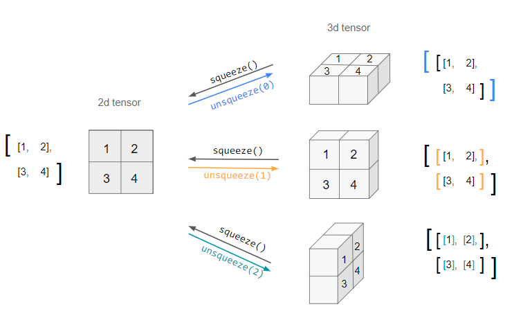
Here is a visual representation of what
torch.squeeze()andtorch.unsqueeze()do for a 2D matrix:
import torch

a = torch.zeros(2, 1, 2, 1, 2)
print(a.size()) # Prints torch.Size([2, 1, 2, 1, 2])

b = torch.squeeze(a)
print(b.size()) # Prints torch.Size([2, 2, 2])

b = torch.squeeze(a, 0)
print(b.size()) # Prints torch.Size([2, 1, 2, 1, 2])

b = torch.squeeze(a, 1)
print(b.size()) # Prints torch.Size([2, 2, 1, 2])
Unsqueeze
-
torch.unsqueeze()is the opposite oftorch.squeeze(). It inserts a dimension of size one at the specified position. The returned tensor shares the same underlying data with this tensor. -
A
dimargument within the range[-input.dim() - 1, input.dim() + 1)can be used. A negative value ofdimwill correspond totorch.unsqueeze()applied atdim = dim + input.dim() + 1.
import torch

a = torch.tensor([1, 2, 3, 4])
print(x.size()) # Prints torch.Size([4])

b = torch.unsqueeze(a, 0)
print(b)        # Prints tensor([[1, 2, 3, 4]])
print(b.size()) # Prints torch.Size([1, 4])

b = torch.unsqueeze(a, 1)
print(b)        # Prints tensor([[1],
                #                [2],
                #                [3],
                #                [4]])
print(b.size()) # torch.Size([4, 1])
-
Note that unlike
torch.squeeze(), thedimargument is required (and not optional) withtorch.unsqueeze(). -
A practical use-case of
torch.unsqueeze()is to add an additional dimension (usually the first dimension) for the batch number as shown in the example below:
import torch

# 3 channels, 32 width, 32 height
a = torch.randn(3, 32, 32)

# 1 batch, 3 channels, 32 width, 32 height
a.unsqueeze(dim=0).shape
Print Model Summary
- Printing the model prints a summary of the model including the different layers involved and their specifications.
from torchvision import models
model = models.vgg16()
print(model)
- The output in this case would be something as follows:
VGG (
  (features): Sequential (
    (0): Conv2d(3, 64, kernel_size=(3, 3), stride=(1, 1), padding=(1, 1))
    (1): ReLU (inplace)
    (2): Conv2d(64, 64, kernel_size=(3, 3), stride=(1, 1), padding=(1, 1))
    (3): ReLU (inplace)
    (4): MaxPool2d (size=(2, 2), stride=(2, 2), dilation=(1, 1))
    (5): Conv2d(64, 128, kernel_size=(3, 3), stride=(1, 1), padding=(1, 1))
    (6): ReLU (inplace)
    (7): Conv2d(128, 128, kernel_size=(3, 3), stride=(1, 1), padding=(1, 1))
    (8): ReLU (inplace)
    (9): MaxPool2d (size=(2, 2), stride=(2, 2), dilation=(1, 1))
    (10): Conv2d(128, 256, kernel_size=(3, 3), stride=(1, 1), padding=(1, 1))
    (11): ReLU (inplace)
    (12): Conv2d(256, 256, kernel_size=(3, 3), stride=(1, 1), padding=(1, 1))
    (13): ReLU (inplace)
    (14): Conv2d(256, 256, kernel_size=(3, 3), stride=(1, 1), padding=(1, 1))
    (15): ReLU (inplace)
    (16): MaxPool2d (size=(2, 2), stride=(2, 2), dilation=(1, 1))
    (17): Conv2d(256, 512, kernel_size=(3, 3), stride=(1, 1), padding=(1, 1))
    (18): ReLU (inplace)
    (19): Conv2d(512, 512, kernel_size=(3, 3), stride=(1, 1), padding=(1, 1))
    (20): ReLU (inplace)
    (21): Conv2d(512, 512, kernel_size=(3, 3), stride=(1, 1), padding=(1, 1))
    (22): ReLU (inplace)
    (23): MaxPool2d (size=(2, 2), stride=(2, 2), dilation=(1, 1))
    (24): Conv2d(512, 512, kernel_size=(3, 3), stride=(1, 1), padding=(1, 1))
    (25): ReLU (inplace)
    (26): Conv2d(512, 512, kernel_size=(3, 3), stride=(1, 1), padding=(1, 1))
    (27): ReLU (inplace)
    (28): Conv2d(512, 512, kernel_size=(3, 3), stride=(1, 1), padding=(1, 1))
    (29): ReLU (inplace)
    (30): MaxPool2d (size=(2, 2), stride=(2, 2), dilation=(1, 1))
  )
  (classifier): Sequential (
    (0): Dropout (p = 0.5)
    (1): Linear (25088 -> 4096)
    (2): ReLU (inplace)
    (3): Dropout (p = 0.5)
    (4): Linear (4096 -> 4096)
    (5): ReLU (inplace)
    (6): Linear (4096 -> 1000)
  )
)
- To get the representation tf.keras offers, use the
pytorch-summarypackage. This contains a lot more details of the model, including:- Name and type of all layers in the model.
- Output shape for each layer.
- Number of weight parameters of each layer.
- The total number of trainable and non-trainable parameters of the model.
- In addition, also offers the following bits not in the Keras summary:
- Input size (MB)
- Forward/backward pass size (MB)
- Params size (MB)
- Estimated Total Size (MB)
from torchvision import models
from torchsummary import summary

# Example for VGG16
vgg = models.vgg16()
summary(vgg, (3, 224, 224))
- The output in this case would be something as follows:
================================================================
        Layer (type)               Output Shape         Param #
================================================================
            Conv2d-1         [-1, 64, 224, 224]           1,792
              ReLU-2         [-1, 64, 224, 224]               0
            Conv2d-3         [-1, 64, 224, 224]          36,928
              ReLU-4         [-1, 64, 224, 224]               0
         MaxPool2d-5         [-1, 64, 112, 112]               0
            Conv2d-6        [-1, 128, 112, 112]          73,856
              ReLU-7        [-1, 128, 112, 112]               0
            Conv2d-8        [-1, 128, 112, 112]         147,584
              ReLU-9        [-1, 128, 112, 112]               0
        MaxPool2d-10          [-1, 128, 56, 56]               0
           Conv2d-11          [-1, 256, 56, 56]         295,168
             ReLU-12          [-1, 256, 56, 56]               0
           Conv2d-13          [-1, 256, 56, 56]         590,080
             ReLU-14          [-1, 256, 56, 56]               0
           Conv2d-15          [-1, 256, 56, 56]         590,080
             ReLU-16          [-1, 256, 56, 56]               0
        MaxPool2d-17          [-1, 256, 28, 28]               0
           Conv2d-18          [-1, 512, 28, 28]       1,180,160
             ReLU-19          [-1, 512, 28, 28]               0
           Conv2d-20          [-1, 512, 28, 28]       2,359,808
             ReLU-21          [-1, 512, 28, 28]               0
           Conv2d-22          [-1, 512, 28, 28]       2,359,808
             ReLU-23          [-1, 512, 28, 28]               0
        MaxPool2d-24          [-1, 512, 14, 14]               0
           Conv2d-25          [-1, 512, 14, 14]       2,359,808
             ReLU-26          [-1, 512, 14, 14]               0
           Conv2d-27          [-1, 512, 14, 14]       2,359,808
             ReLU-28          [-1, 512, 14, 14]               0
           Conv2d-29          [-1, 512, 14, 14]       2,359,808
             ReLU-30          [-1, 512, 14, 14]               0
        MaxPool2d-31            [-1, 512, 7, 7]               0
           Linear-32                 [-1, 4096]     102,764,544
             ReLU-33                 [-1, 4096]               0
          Dropout-34                 [-1, 4096]               0
           Linear-35                 [-1, 4096]      16,781,312
             ReLU-36                 [-1, 4096]               0
          Dropout-37                 [-1, 4096]               0
           Linear-38                 [-1, 1000]       4,097,000
================================================================
Total params: 138,357,544
Trainable params: 138,357,544
Non-trainable params: 0
-
Input size (MB): 0.57
Forward/backward pass size (MB): 218.59
Params size (MB): 527.79
Estimated Total Size (MB): 746.96
-
Got it. Below is the same section, but with inline end-of-line comments (aligned and indented in the same style as the rest of the primer), instead of block comments.
You can drop this directly into the document.
Keepdim (Keeping Reduced Dimensions)
-
While not a PyTorch function,
keepdimis an argument commonly used across many PyTorch reduction operations (e.g.,sum,mean,max,min,argmax) reduce the dimensionality of a tensor by default. Settingkeepdim=Truepreserves the reduced dimension with size 1 instead of removing it. -
This is especially important when:
- You want consistent tensor ranks throughout a pipeline
- You rely on broadcasting in later operations
- You want to avoid manual reshaping with
unsqueeze() - You compute batch-wise statistics, normalization, masking, or attention scores
-
By default, reduced dimensions are removed. Using
keepdim=Truekeeps those dimensions as size-1 axes, preventing shape mismatches and making downstream code simpler and more readable.
Basic Syntax
torch.sum(input, dim=..., keepdim=True)
torch.mean(input, dim=..., keepdim=True)
torch.max(input, dim=..., keepdim=True)
Example 1: Sum With and Without keepdim
import torch

x = torch.tensor([[1., 2., 3.],
                  [4., 5., 6.]])       # tensor([[1., 2., 3.],
                                       #         [4., 5., 6.]])

s1 = torch.sum(x, dim=1)               # tensor([ 6., 15.])
s1.shape                               # torch.Size([2])

s2 = torch.sum(x, dim=1, keepdim=True) # tensor([[ 6.],
                                       #         [15.]])
s2.shape                               # torch.Size([2, 1])
-
Interpretation:
keepdim=False\(\rightarrow\) shape(2)keepdim=True\(\rightarrow\) shape(2, 1)
Example 2: Mean and Broadcasting
x = torch.randn(4, 5)                   # shape: torch.Size([4, 5])

mean_no_keep = x.mean(dim=1)            # shape: torch.Size([4])
mean_keep = x.mean(dim=1, keepdim=True) # shape: torch.Size([4, 1])

y1 = x - mean_no_keep                   # RuntimeError (shape mismatch)
y2 = x - mean_keep                      # shape: torch.Size([4, 5])
-
Why this works:
(4,5) - (4,)cannot broadcast(4,5) - (4,1)broadcasts across columns
Example 3: Max Values and Indices
x = torch.tensor([[1., 7., 3.],
                  [4., 2., 9.]]) # tensor([[1., 7., 3.],
                                 #         [4., 2., 9.]])

values, indices = torch.max(x, dim=1, keepdim=True)

values                           # tensor([[7.],
                                 #         [9.]])
indices                          # tensor([[1],
                                 #         [2]])
- Both outputs preserve the reduced dimension.
Example 4: keepdim vs. unsqueeze
a = x.sum(dim=1, keepdim=True) # shape: torch.Size([2, 1])
b = x.sum(dim=1).unsqueeze(1)  # shape: torch.Size([2, 1])
- Both are equivalent, but
keepdim=Trueis shorter and clearer.
End-to-End Data to Model Pipeline
-
Modern machine learning systems rely on a carefully orchestrated sequence of stages that transform raw, unstructured data into trained, deployable models capable of inference and decision-making. This end-to-end data-to-model pipeline is the backbone of both research experimentation and production-scale AI systems. It ensures that data is consistently prepared, models are trained reproducibly, and evaluations are conducted rigorously across multiple iterations of experimentation.
-
At a high level, the pipeline consists of five interconnected stages:
- Data Pre-processing: cleaning, transforming, and structuring raw inputs into a model-ready format.
- Model Definition and Architecture Design: implementing the neural network or algorithm that will learn from the data.
- Training Loop and Optimization: defining how the model learns via loss computation, backpropagation, and gradient updates.
- Evaluation and Validation: measuring model performance using appropriate metrics and datasets.
- Deployment and Monitoring: serving trained models in production and tracking their behavior over time.
-
Each component in this chain depends on the quality and reproducibility of the previous step. For example, inconsistencies in preprocessing—such as incorrect normalization or tokenization—can lead to unstable training or biased model behavior downstream. Conversely, well-engineered preprocessing pipelines can significantly accelerate convergence and improve generalization.
-
In practice, PyTorch provides a flexible ecosystem that supports every stage of this workflow. It offers modular abstractions for dataset handling (
torch.utils.data), model construction (torch.nn.Module), training orchestration (torch.optim,torch.autograd), and evaluation tools. Together, these modules enable practitioners to prototype and scale ML pipelines efficiently, from experimental notebooks to distributed training environments. -
The first and most foundational stage—data pre-processing—lays the groundwork for all subsequent steps. It determines how efficiently the model can learn meaningful patterns from input data. The following section explores this phase in depth, detailing the principles, abstractions, and best practices for pre-processing both NLP, vision, and audio datasets in PyTorch.
Data Pre-processing
Overview
-
Data pre-processing is the first and most critical step in the deep learning pipeline. In PyTorch, pre-processing prepares raw input (images, text, tabular, or multimodal) into a form suitable for tensors, which are the basic data units that neural networks operate on.
-
Poorly pre-processed data often leads to:
- Slower convergence or failure to converge.
- Model overfitting or underfitting.
- Poor generalization.
-
The pre-processing stage differs for images, text, and audio, but shares the same conceptual flow:
- Loading raw data from disk or external sources.
- Cleaning — handling missing, noisy, or invalid samples.
- Transformation — resizing, normalization, encoding, or augmentation.
- Conversion to tensors compatible with the model.
- Batch preparation for efficient GPU computation.
Key Abstractions for Pre-processing
torch.utils.data.Dataset
- Abstract class representing a dataset.
-
You subclass it and override:
__len__: returns the number of samples.__getitem__: returns a single data sample.
torchtext.transforms
-
Purpose: Provides composable, production-ready text pre-processing utilities that convert raw textual data into tensor representations for NLP models.
-
Key capabilities include:
-
Tokenization and normalization:
- Split raw text into tokens using pretrained tokenizers (e.g., BERT, GPT2) or custom tokenization pipelines.
- Case normalization, punctuation removal, and optional subword encoding.
-
Vocabulary and numericalization:
VocabTransformmaps tokens to integer IDs using a defined vocabulary.- Supports handling of unknown (
<unk>) and padding (<pad>) tokens. - Facilitates training of embeddings and transformer-based models.
-
Padding and sequence management:
Truncate,PadTransform, andToTensorstandardize sequence lengths for batching.- Enables easy collation using
torchtext.functional.to_tensor()or custom collate functions.
-
Composable transform chains:
- Similar to
torchvision, multiple text transformations can be chained usingtorchtext.transforms.Sequential.
- Similar to
-
-
Example:
from torchtext import transforms
from torchtext.vocab import build_vocab_from_iterator

# Custom augmentation functions
class RandomWordDropout:
    """Randomly drops words with a given probability."""
    def __init__(self, p=0.1):
        self.p = p

    def __call__(self, tokens):
        return [tok for tok in tokens if random.random() > self.p]

class SynonymReplacement:
    """Simple synonym replacement using a lookup dictionary."""
    def __init__(self, synonym_dict, p=0.1):
        self.synonym_dict = synonym_dict
        self.p = p

    def __call__(self, tokens):
        augmented = []
        for tok in tokens:
            if tok in self.synonym_dict and random.random() < self.p:
                augmented.append(random.choice(self.synonym_dict[tok]))
            else:
                augmented.append(tok)
        return augmented

# Example synonym mapping
synonyms = {
    "good": ["great", "excellent", "nice"],
    "bad": ["terrible", "awful", "poor"]
}

# Suppose 'vocab' is built from your corpus
vocab = build_vocab_from_iterator([["this", "is", "a", "good", "sample"]], specials=["<unk>", "<pad>"])
vocab.set_default_index(vocab["<unk>"])

text_transform = transforms.Sequential(
    # Step 1: Randomly replace words with synonyms (30% probability)
    SynonymReplacement(synonyms, p=0.3),

    # Step 2: Randomly drop words from the sequence (20% probability)
    RandomWordDropout(p=0.2),

    # Step 3: Convert tokens into integer IDs using the predefined vocabulary
    transforms.VocabTransform(vocab),

    # Step 4: Truncate sequences longer than 512 tokens to a fixed maximum length
    transforms.Truncate(512),

    # Step 5: Convert the list of token IDs into a tensor and pad to uniform length
    transforms.ToTensor(padding_value=vocab['<pad>'])
)

tokens = ["this", "is", "a", "sample"]
tensorized = text_transform(tokens)
-
Integration with data pipeline:
- Used in NLP datasets like IMDB, AG News, or custom text corpora.
- Can be combined with
torch.utils.data.Datasetfor tokenized text pipelines and efficient batch collation. - Outputs tensors compatible with RNNs, CNNs, and Transformer architectures.
torchvision.transforms
-
Purpose: Handles image and video transformations efficiently, both for data normalization and augmentation during training. It provides a powerful composition framework for chaining multiple transformations using
transforms.Compose. -
Key capabilities include:
-
Geometric transformations:
Resize,CenterCrop,RandomCrop,RandomHorizontalFlip,Rotate, etc.- Commonly used for resizing images to match model input size and augmenting data variability.
-
Color and intensity transformations:
Normalize,ColorJitter,Grayscale,RandomAdjustSharpness, etc.- Used to adjust brightness, contrast, saturation, and sharpness for robustness.
-
Tensor conversion and PIL integration:
ToTensor()converts a PIL image or NumPy array to a normalized PyTorch tensor (values scaled to [0, 1]).ToPILImage()allows converting back to image format for visualization.
-
Augmentation pipelines:
- Supports stochastic transformations during training for better generalization.
RandomApplyandRandomChoicecan randomize transform sequences.
-
Video support:
- Extended transforms for temporal augmentation (
RandomResizedCropVideo,NormalizeVideo, etc.) intorchvision.transforms._transforms_video.
- Extended transforms for temporal augmentation (
-
-
Example:
from torchvision import transforms

image_transform = transforms.Compose([
    # Step 1: Resize the input image so the shorter side is 256 pixels
    transforms.Resize(256),

    # Step 2: Crop the central 224×224 region from the resized image
    transforms.CenterCrop(224),

    # Step 3: Randomly flip the image horizontally (helps with data augmentation)
    transforms.RandomHorizontalFlip(),

    # Step 4: Convert the PIL image to a PyTorch tensor and scale pixel values to [0, 1]
    transforms.ToTensor(),

    # Step 5: Normalize tensor using ImageNet channel means and standard deviations
    #         (this standardization helps models pretrained on ImageNet converge better)
    transforms.Normalize(mean=[0.485, 0.456, 0.406],
                         std=[0.229, 0.224, 0.225])
])
-
Integration with data pipeline:
- Used inside the
__getitem__method of aDatasetsubclass to ensure each image is transformed at load time. - The transformed tensors can then be directly batched using
torch.utils.data.DataLoaderfor efficient GPU training.
- Used inside the
torchaudio.transforms
-
Purpose: Provides transformations and utilities for audio signal processing, converting raw waveforms into representations suitable for neural networks.
-
Key capabilities include:
-
Waveform transformations:
Resample,Vol,TimeStretch,PitchShift, etc.- Used to adjust sampling rates, tempo, and pitch or to augment data diversity.
-
Spectrogram and feature extraction:
Spectrogram,MelSpectrogram,MFCC,AmplitudeToDB.- Convert time-domain waveforms into frequency-domain features.
- Common in ASR (Automatic Speech Recognition) and music analysis.
-
Augmentation and masking:
FrequencyMasking,TimeMaskinghelp simulate noise and missing information for better generalization.- Especially beneficial in low-resource audio tasks.
-
I/O integration:
torchaudio.load()reads and returns(waveform, sample_rate)directly as tensors.- Supports a variety of audio formats (WAV, MP3, FLAC, etc.).
-
-
Example:
import torchaudio
from torchaudio import transforms as T

waveform, sample_rate = torchaudio.load("speech.wav")

audio_transform = T.Compose([
    # Step 1: Resample the raw audio waveform to a consistent 16 kHz sampling rate
    T.Resample(orig_freq=sample_rate, new_freq=16000),

    # Step 2: Convert the waveform into a Mel-spectrogram (frequency–time representation)
    # Uses 64 Mel filter banks to capture perceptually relevant frequency information
    T.MelSpectrogram(sample_rate=16000, n_mels=64),

    # Step 3: Apply frequency masking (randomly masks frequency bands)
    # Helps the model generalize to variations in spectral features
    T.FrequencyMasking(freq_mask_param=15),

    # Step 4: Apply time masking (randomly masks time segments)
    # Improves robustness to temporal distortions or missing frames
    T.TimeMasking(time_mask_param=35),

    # Step 5: Convert the Mel-spectrogram power values to decibel (dB) scale
    # Produces log-scaled features commonly used in speech and audio models
    T.AmplitudeToDB()
])

mel_spectrogram = audio_transform(waveform)
-
Integration with training pipeline:
- The transformed tensor (
mel_spectrogram) can be directly used as input for CNN or Transformer-based models. - Seamlessly integrates with
torch.utils.data.Datasetfor dynamic, on-the-fly augmentation during data loading. - Suitable for tasks such as speech recognition, audio classification, or speaker verification.
- The transformed tensor (
torch.utils.data.DataLoader
-
Takes a
Datasetand handles:- Batching
- Shuffling
- Parallel loading using
num_workers
-
Essential for GPU efficiency (avoids CPU bottlenecks).
Pre-processing for Vision Data
Loading and Cleaning
- Image data are typically in JPEG or PNG format.
-
Cleaning includes:
- Removing corrupt files.
- Ensuring consistent channels (e.g., converting grayscale to RGB).
- Resizing to a common resolution (e.g., 224×224).
Normalization
- Neural networks perform best when inputs are normalized to zero mean and unit variance.
-
For an image tensor \(I\) with pixel values in \([0, 1]\):
\[I' = \frac{I - \mu}{\sigma}\]- where \(\mu\) and \(\sigma\) are per-channel means and standard deviations.
- Typical ImageNet normalization constants:
mean = [0.485, 0.456, 0.406]
std  = [0.229, 0.224, 0.225]
Data Augmentation
-
Used to increase the diversity of training examples and reduce overfitting.
-
Common augmentations:
RandomResizedCropColorJitterRandomHorizontalFlipRandomRotationRandomErasing
-
See torchvision.transforms documentation for the full list.
Conversion to Tensor
- Convert PIL images to PyTorch tensors in \([C, H, W]\) format.
- Scale pixel values to \([0, 1]\) using
ToTensor().
Pre-processing for Text Data
Tokenization
- Tokenization splits raw text into tokens.
-
Modern NLP pipelines often use subword tokenization methods, such as:
- Example sentence:
“PyTorch is awesome!”
\(\rightarrow\) Tokens:
["pytorch", "is", "awesome", "!"]
Vocabulary Building
-
Each unique token gets mapped to an integer ID.
-
Example:
{'<PAD>':0, '<UNK>':1, 'pytorch':2, 'is':3, 'awesome':4, '!':5}
Handling Variable-Length Sequences
-
Different sentences have different lengths — we pad or truncate to a fixed length \(L\).
- If sentence length < \(L\) \(\rightarrow\) pad with
<PAD>tokens. - If sentence length > \(L\) \(\rightarrow\) truncate.
- If sentence length < \(L\) \(\rightarrow\) pad with
Embedding Lookup
-
Each token index is converted into a dense vector representation:
\[x_i = E[w_i]\]- where \(E\) is the embedding matrix and \(w_i\) is the token index.
-
This is handled in PyTorch with:
nn.Embedding(num_embeddings, embedding_dim)
Masking
- A mask tensor marks which tokens are padding. This ensures that padding tokens don’t contribute to loss or attention weights during training.
Pre-processing for Audio Data
Loading and Cleaning
-
Audio data are typically stored in WAV, MP3, or FLAC formats.
-
PyTorch provides
torchaudio.load()for direct reading of these files, returning a tuple(waveform, sample_rate)where the waveform is a tensor of shape[channels, time]. -
Common cleaning steps include:
- Removing or skipping corrupted audio files.
- Resampling all clips to a consistent sample rate (e.g., 16 kHz) for uniformity.
- Converting stereo audio to mono when multi-channel information is not required.
- Trimming or padding clips to a fixed duration for batch processing.
import torchaudio

waveform, sample_rate = torchaudio.load("speech.wav")
waveform = torchaudio.functional.resample(waveform, orig_freq=sample_rate, new_freq=16000)
Normalization (Standardization)
-
Normalization ensures that the waveform amplitude is within a suitable numeric range for stable learning. A common approach, known as standardization, rescales the waveform to have zero mean and unit variance, as given by
\[x' = \frac{x - \mu}{\sigma}\]- where \(\mu\) and \(\sigma\) are the mean and standard deviation of the waveform.
- This process ensures that all samples contribute equally during training.
-
Alternatively, amplitude can be normalized by dividing by the maximum absolute value to fit within \([-1, 1]\), which preserves the waveform’s relative shape but constrains its dynamic range.
-
After transformation into spectrograms, normalization is often applied in decibel space using:
T.AmplitudeToDB()
Feature Extraction
-
Raw waveforms are not directly suitable for many deep learning models. They are typically converted into time–frequency representations that capture spectral features.
-
Common feature transforms:
Spectrogram: Converts waveform to magnitude-frequency domain.MelSpectrogram: Maps frequencies onto the Mel scale for perceptual alignment.MFCC: Computes Mel-Frequency Cepstral Coefficients, widely used in speech recognition.DeltaandDeltaDelta: Compute first and second derivatives to capture temporal change.
from torchaudio import transforms as T

audio_transform = T.MelSpectrogram(
    sample_rate=16000,
    n_mels=64,
    n_fft=1024,
    hop_length=256
)
mel_spectrogram = audio_transform(waveform)
Data Augmentation
-
Audio augmentation increases data diversity and improves generalization under noisy or varied recording conditions.
-
Common augmentations include:
-
SpecAugment techniques:
FrequencyMasking(freq_mask_param=15)— randomly masks frequency bands.TimeMasking(time_mask_param=35)— randomly masks time intervals.
-
Temporal transforms:
TimeStretch— changes speed without affecting pitch.PitchShift— alters pitch while preserving duration.
-
Amplitude transforms:
Vol— adjusts loudness levels randomly.
-
-
Example:
from torchaudio import transforms as T

augment = T.Compose([
    T.FrequencyMasking(freq_mask_param=15),
    T.TimeMasking(time_mask_param=35),
    T.Vol(gain=(0.5, 1.5))
])
augmented_spectrogram = augment(mel_spectrogram)
Conversion to Tensor and Batching
-
Audio tensors are already returned in PyTorch’s tensor format by
torchaudio.load(). -
For batch processing, shorter clips are padded and longer clips truncated to maintain consistent time dimensions.
-
Batched tensors follow shape
[batch_size, channels, time]for waveform inputs or[batch_size, channels, freq, time]for spectrograms. -
Padding can be applied using:
torch.nn.utils.rnn.pad_sequence(list_of_waveforms, batch_first=True)
Integration with Models
-
After pre-processing, tensors can be fed into:
- CNNs (for spectrogram-based classification).
- RNNs or Transformers (for speech recognition).
- Pretrained audio encoders such as Wav2Vec2, HuBERT, or Whisper.
Data Quality Checks
-
Before proceeding to model training:
- Verify dataset split integrity (train/val/test non-overlap).
- Visualize samples to catch label mismatches.
- Ensure normalization and padding/truncation logic works as expected.
- Detect data imbalance and decide on resampling or weighted losses.
-
A detailed discourse on data quality can be found in our Data Quality/Filtering primer.
Tabular Summary
| Modality | Key Steps | Common Transforms | Notes |
|---|---|---|---|
| Text | Tokenize $$\rightarrow$$ Augment $$\rightarrow$$ Numericalize $$\rightarrow$$ Pad $$\rightarrow$$ Mask | SynonymReplacement, RandomWordDropout, NoiseInjection, VocabTransform, Truncate, PadTransform |
Apply augmentation before numericalization; handle OOVs with <UNK> |
| Vision | Resize $$\rightarrow$$ Normalize $$\rightarrow$$ Augment $$\rightarrow$$ Tensor | Resize, Normalize, ToTensor, RandomCrop |
Use per-channel normalization |
| Audio | Load $$\rightarrow$$ Resample $$\rightarrow$$ Feature Extract $$\rightarrow$$ Augment $$\rightarrow$$ Normalize | MelSpectrogram, AmplitudeToDB, FrequencyMasking, TimeMasking |
Ensure consistent sampling rate and duration |
| Shared | Cleaning, batching, shuffling | Dataset, DataLoader |
Use multiprocessing in DataLoader |
FAQs
- Why do we normalize image data, and why are the ImageNet mean/std values often used as defaults?
- Normalization stabilizes learning by ensuring all features have similar dynamic ranges. ImageNet’s statistics are widely used because many pretrained models are trained on ImageNet, and maintaining the same normalization helps when fine-tuning those models.
- What happens if you skip padding for NLP data?
- Batches cannot be represented as tensors since tensors require fixed dimensions. Without padding, PyTorch cannot stack sentences of different lengths into a batch tensor.
- Why do we use subword tokenization instead of simple whitespace tokenization?
- Subword tokenization handles out-of-vocabulary (OOV) words and rare word morphologies better. It splits unknown or compound words into smaller known units, improving generalization.
- Why is data augmentation not applied during evaluation?
- Augmentation introduces randomness intended for training robustness. During evaluation, we need deterministic, unaltered inputs to measure model performance consistently.
References and Further Reading
- PyTorch official docs: torch.utils.data
- torchtext.transforms
- torchvision.transforms
- torchaudio.transforms documentation
- SpecAugment: A Simple Data Augmentation Method for Speech Recognition (Park et al., 2019)
- Wav2Vec 2.0: A Framework for Self-Supervised Learning of Speech Representations (Baevski et al., 2020)
- A Guide to PyTorch Data Loading
- Understanding WordPiece and BPE Tokenization
- BPE by Sennrich et al. (2016)
- SentencePiece by Kudo & Richardson (2018)
Practical Implementation – Data Pre-processing
- This section shows two fully worked examples: one for NLP and one for Vision, followed by a FAQs section for conceptual discussion.
NLP Data Pre-processing – Text Classification Example
- Below is a simple pre-processing pipeline for a text classification dataset using
torchtext.
import torch
from torch.utils.data import Dataset, DataLoader
from torchtext.vocab import build_vocab_from_iterator
from torch.nn.utils.rnn import pad_sequence
import re

# ----------------------------------------------------------
# 1. Tokenizer
# ----------------------------------------------------------
# - Purpose: Convert raw text into a list of clean tokens (words).
# - Steps:
#     * Convert text to lowercase for uniformity.
#     * Remove all punctuation and special characters using regex.
#     * Split text into individual word tokens (by whitespace).
def tokenize(text):
    text = re.sub(r"[^a-zA-Z0-9\s]", "", text.lower())
    return text.split()

# ----------------------------------------------------------
# 2. Sample corpus
# ----------------------------------------------------------
# - Example dataset for binary classification (e.g., sentiment, relevance).
# - Each text string corresponds to one data sample, with label 0 or 1.
texts = [
    "Large Language Models are powerful AI models",
    "Deep learning is transformational",
    "Neural networks can generalize",
    "PyTorch simplifies model training"
]
labels = [1, 0, 1, 0]

# ----------------------------------------------------------
# 3. Build vocabulary
# ----------------------------------------------------------
# - The vocabulary assigns each unique token an integer index.
# - This is critical for converting tokens into numerical form that models can process.
# - The special tokens:
#     * <pad>: used for sequence padding (makes sequences same length in a batch).
#     * <unk>: represents out-of-vocabulary tokens (unknown words).
vocab = build_vocab_from_iterator(map(tokenize, texts), specials=["<pad>", "<unk>"])
vocab.set_default_index(vocab["<unk>"])  # All unseen tokens map to <unk>

# ----------------------------------------------------------
# 4. Numericalization
# ----------------------------------------------------------
# - Converts a list of string tokens into a tensor of integer IDs using the vocabulary.
# - Example:
#   Input:  ["deep", "learning", "is", "transformational"]
#   Output: tensor([5, 9, 3, 8])  # based on vocab indices
def numericalize(text):
    return torch.tensor([vocab[token] for token in tokenize(text)], dtype=torch.long)

# ----------------------------------------------------------
# 5. Dataset definition
# ----------------------------------------------------------
# - Custom Dataset class wraps the tokenized text and corresponding labels.
# - Required methods:
#     * __getitem__(self, idx): returns one sample (text tensor, label tensor).
#     * __len__(self): returns total number of samples.
class TextDataset(Dataset):
    def __init__(self, texts, labels):
        self.texts = texts
        self.labels = labels

    def __getitem__(self, idx):
        # Returns a tuple: (numericalized text tensor, label tensor)
        return numericalize(self.texts[idx]), torch.tensor(self.labels[idx])

    def __len__(self):
        return len(self.texts)

# Instantiate dataset object
dataset = TextDataset(texts, labels)

# ----------------------------------------------------------
# 6. Collate function for padding
# ----------------------------------------------------------
# - Purpose: dynamically pad variable-length text sequences in a batch.
# - pad_sequence: ensures all sequences in the batch are the same length.
# - padding_value: index corresponding to <pad> token in the vocabulary.
def collate_fn(batch):
    # Unzip the batch (list of (text, label) pairs) into separate sequences and labels
    texts, labels = zip(*batch)
    # Pad sequences so all have equal length (batch_first=True $$\rightarrow$$ shape [batch, seq_len])
    padded = pad_sequence(texts, batch_first=True, padding_value=vocab["<pad>"])
    # Stack labels into a single tensor
    return padded, torch.stack(labels)

# ----------------------------------------------------------
# 7. DataLoader
# ----------------------------------------------------------
# - Combines dataset and collate function to create mini-batches.
# - Handles:
#     * Shuffling for random sampling each epoch.
#     * Batch creation.
#     * Optional parallel data loading via num_workers.
loader = DataLoader(dataset, batch_size=2, collate_fn=collate_fn, shuffle=True)

# ----------------------------------------------------------
# 8. Inspect one mini-batch
# ----------------------------------------------------------
# - Demonstrates the final structure after pre-processing.
# - Each batch has:
#     * x_batch: tensor of shape [batch_size, sequence_length]
#     * y_batch: tensor of shape [batch_size]
for x_batch, y_batch in loader:
    print(f"Input batch shape: {x_batch.shape}")  # e.g., (2, seq_len)
    print(f"Label batch shape: {y_batch.shape}")  # e.g., (2,)
    break

# Can also do the following in place of the above block:
# ----------------------------------------------------------
# 8. Inspect one mini-batch (using next(iter(loader)))
# ----------------------------------------------------------
# - Demonstrates how to manually fetch a single batch from a DataLoader.
# - This approach is equivalent to running one iteration of the loop.
# - Useful for debugging or inspecting batch structure and tensor shapes using one batch only.

# Create an iterator over the DataLoader
# batch_iter = iter(loader)

# Fetch the first batch (x_batch, y_batch)
# x_batch, y_batch = next(batch_iter)

# Inspect the shapes of tensors
# print(f"Input batch shape: {x_batch.shape}")   # e.g., (2, seq_len)
# print(f"Label batch shape: {y_batch.shape}")   # e.g., (2,)
-
Concepts Illustrated:
- Text cleaning and tokenization.
- Vocabulary building and OOV handling.
- Batch collation with dynamic padding using
pad_sequence. - Labels and sequences packed into tensors ready for embedding lookup.
Vision Data Pre-processing – CIFAR-10 Example
- This example uses torchvision to build a reusable pre-processing and data-loading pipeline.
import torch
from torchvision import datasets, transforms
from torch.utils.data import DataLoader

# ----------------------------------------------------------
# 1. Define data transformations
# ----------------------------------------------------------
# These define how images are preprocessed before feeding into the model.
# Training transforms include augmentations for better generalization,
# while validation/test transforms remain deterministic for fair evaluation.

train_transforms = transforms.Compose([
    transforms.RandomHorizontalFlip(),     # Randomly flip images horizontally (helps learn invariance)
    transforms.RandomRotation(10),         # Apply small random rotations to simulate varied orientations
    transforms.ToTensor(),                 # Convert PIL image $$\rightarrow$$ Tensor with shape (C, H, W), values in [0,1]
    transforms.Normalize(mean=(0.5, 0.5, 0.5),  # Normalize RGB channels (center around 0, scale to ~[-1,1])
                         std=(0.5, 0.5, 0.5))
])

test_transforms = transforms.Compose([
    transforms.ToTensor(),                 # Convert test images to tensor (no random augmentations)
    transforms.Normalize(mean=(0.5, 0.5, 0.5),
                         std=(0.5, 0.5, 0.5))
])

# ----------------------------------------------------------
# 2. Load dataset
# ----------------------------------------------------------
# Automatically downloads and prepares CIFAR-10 dataset if not already present.
# - train=True $$\rightarrow$$ loads training split (50,000 images)
# - train=False $$\rightarrow$$ loads test split (10,000 images)
# - transform=... $$\rightarrow$$ applies preprocessing pipeline on-the-fly
train_data = datasets.CIFAR10(root='data', train=True, download=True, transform=train_transforms)
test_data = datasets.CIFAR10(root='data', train=False, download=True, transform=test_transforms)

# ----------------------------------------------------------
# 3. Prepare DataLoaders
# ----------------------------------------------------------
# DataLoader efficiently handles batching, shuffling, and multiprocessing.
# - batch_size=64 $$\rightarrow$$ each batch contains 64 images
# - shuffle=True $$\rightarrow$$ reshuffles data at each epoch to reduce overfitting
# - num_workers=4 $$\rightarrow$$ uses 4 subprocesses for parallel data loading
train_loader = DataLoader(train_data, batch_size=64, shuffle=True, num_workers=4)
test_loader = DataLoader(test_data, batch_size=64, shuffle=False, num_workers=4)

# ----------------------------------------------------------
# 4. Inspect one batch
# ----------------------------------------------------------
# Retrieve a single mini-batch using an iterator.
# - iter(train_loader) returns an iterator over batches
# - next(...) yields the first batch (images and labels)
images, labels = next(iter(train_loader))

# Print tensor shapes for verification
# CIFAR-10 images: (64 samples, 3 color channels, 32x32 resolution)
print(f"Batch shape: {images.shape}")  # Expected $$\rightarrow$$ (64, 3, 32, 32)
print(f"Label shape: {labels.shape}")  # Expected $$\rightarrow$$ (64,)
-
Concepts Illustrated:
- Data augmentation (
RandomHorizontalFlip,RandomRotation) only applied to training data. - Normalization keeps values in a range suitable for model convergence.
DataLoaderbatches and parallelizes loading withnum_workers.
- Data augmentation (
FAQs
- Why separate train and test transforms in vision pipelines?
- Training transformations (augmentations) simulate data diversity and improve generalization. Test transforms must be deterministic to ensure consistent evaluation metrics.
- Why is normalization critical before feeding data into a neural network?
- Normalization standardizes feature scales. It keeps gradients balanced during backpropagation and helps models converge faster. Without it, models may learn unstable weight updates.
- Why use
num_workers > 0in DataLoader?- Setting
num_workersallows data loading to happen in parallel across CPU cores. This prevents the GPU from idling while waiting for batches to be loaded and preprocessed.
- Setting
- What is the purpose of a custom
collate_fnin NLP DataLoaders?- Sequences vary in length.
collate_fnpads sequences to a fixed length per batch so that they can be stacked into a tensor, while also optionally creating masks to ignore padding during loss computation.
- Sequences vary in length.
- How can you extend this pipeline for multilingual text?
- Integrate tokenizers like SentencePiece or HuggingFace’s AutoTokenizer, trained on multilingual corpora. SentencePiece handles text as raw byte sequences, making it more language-agnostic and effective for languages without clear word boundaries. AutoTokenizer is useful because it automatically loads the correct pretrained tokenizer configuration (e.g., BPE, WordPiece, or SentencePiece) for multilingual models, simplifying setup and ensuring compatibility.
- Why not pre-pad all sequences globally before training?
- Global padding wastes computation and memory for short sentences. Dynamic per-batch padding (via
collate_fn) ensures efficiency while preserving batch-level alignment.
- Global padding wastes computation and memory for short sentences. Dynamic per-batch padding (via
- What happens if we forget to call
.set_default_index()for<unk>tokens?- Any out-of-vocabulary token will raise an error instead of mapping to
<unk>. This breaks robustness when unseen words appear during validation or inference.
- Any out-of-vocabulary token will raise an error instead of mapping to
- Why use
ToTensor()afterPILtransforms?ToTensor()converts the image from \([H, W, C]\) format with pixel values in \([0, 255]\) to \([C, H, W]\) format with normalized floats in \([0, 1]\). PyTorch models expect this tensor format.
- What are alternatives to torchvision for custom vision datasets?
PilloworOpenCVfor manual image preprocessing.albumentationsfor advanced augmentations (blur, affine transformations, contrast shifts).- Custom PyTorch transforms for domain-specific needs (e.g., medical images, satellite imagery).
- How can you visualize pre-processed batches for debugging?
- Use
matplotlibto plot a few tensor samples:
import matplotlib.pyplot as plt import torchvision images, _ = next(iter(train_loader)) grid = torchvision.utils.make_grid(images[:8], nrow=4) plt.imshow(grid.permute(1, 2, 0)) plt.show()- Visual inspection is crucial to confirm augmentations and normalization behave as intended.
- Use
Model Training/Fine-tuning and Evaluation Workflow
- This section walks through training loop design, fine-tuning using LoRA, evaluation strategies, and monitoring techniques in PyTorch, with code and conceptual explanations.
Overview
-
After pre-processing, the next phase in an ML pipeline is model training and evaluation.
-
The goals here are:
- Define model architectures suitable for the task.
- Build a robust and efficient training loop.
- Evaluate performance and prevent overfitting.
- Save and restore model checkpoints.
-
A well-structured training and evaluation workflow ensures reproducibility, scalability, and easier debugging.
Core Components of a Training Workflow
-
A minimal PyTorch training pipeline has these components:
- Model Definition – subclass
nn.Module. - Loss Function – e.g., CrossEntropyLoss for classification.
- Optimizer – e.g., Adam or SGD.
- Training Loop – iterate over batches, compute loss, and update weights.
- Validation Loop – measure generalization performance.
- Checkpointing – save the best model.
- Early Stopping – stop training when validation stops improving.
- Model Definition – subclass
Example: NLP Model Training Workflow
- Here’s a lightweight text classification model using embeddings and an RNN.
import torch
import torch.nn as nn
import torch.optim as optim

# ----------------------------------------------------------
# 1. Define RNN-based text classification model
# ----------------------------------------------------------
class RNNClassifier(nn.Module):
    def __init__(self, vocab_size, embed_dim, hidden_dim, num_classes, pad_idx):
        super().__init__()
        # Embedding layer converts token IDs into dense vector representations
        self.embedding = nn.Embedding(vocab_size, embed_dim, padding_idx=pad_idx)

        # GRU captures temporal dependencies in token sequences
        self.rnn = nn.GRU(embed_dim, hidden_dim, batch_first=True)

        # Fully connected output layer for classification logits
        self.fc = nn.Linear(hidden_dim, num_classes)

    def forward(self, x):
        # x shape: (batch_size, seq_len)
        embedded = self.embedding(x)     # $$\rightarrow$$ (batch_size, seq_len, embed_dim)
        _, h = self.rnn(embedded)        # h: (1, batch_size, hidden_dim)
        return self.fc(h.squeeze(0))     # $$\rightarrow$$ (batch_size, num_classes)


# ----------------------------------------------------------
# 2. Instantiate model, loss, and optimizer
# ----------------------------------------------------------
vocab_size = len(vocab)  # Number of tokens in vocabulary
model = RNNClassifier(
    vocab_size=vocab_size,
    embed_dim=64,
    hidden_dim=128,
    num_classes=2,
    pad_idx=vocab["<pad>"]
)

criterion = nn.CrossEntropyLoss()               # Cross-entropy for classification
optimizer = optim.Adam(model.parameters(), lr=1e-3)  # Adaptive optimizer


# ----------------------------------------------------------
# 3. Define Evaluation Function (Validation Loop)
# ----------------------------------------------------------
def evaluate_nlp_model(model, loader, criterion):
    """
    Evaluates model performance on a validation or test DataLoader.
    Returns average loss and accuracy.
    """
    model.eval()  # Disable dropout, batchnorm updates
    total_loss, correct, total = 0.0, 0, 0

    with torch.no_grad():  # Disable gradient computation for faster inference
        for x_batch, y_batch in loader:
            outputs = model(x_batch)
            loss = criterion(outputs, y_batch)
            total_loss += loss.item()

            # Get predicted labels (index of max logit)
            preds = outputs.argmax(dim=1)
            correct += (preds == y_batch).sum().item()
            total += y_batch.size(0)

    avg_loss = total_loss / len(loader)
    accuracy = correct / total
    return avg_loss, accuracy


# ----------------------------------------------------------
# 4. Define Training Loop
# ----------------------------------------------------------
def train_nlp_model(model, train_loader, val_loader, criterion, optimizer, epochs=5):
    """
    Trains the NLP model and evaluates on validation data per epoch.
    """
    best_val_loss = float('inf')

    for epoch in range(epochs):
        model.train()  # Enable training mode
        total_loss = 0.0

        # Loop over mini-batches
        for x_batch, y_batch in train_loader:
            optimizer.zero_grad()
            outputs = model(x_batch)
            loss = criterion(outputs, y_batch)
            loss.backward()
            optimizer.step()
            total_loss += loss.item()

        # Compute average training loss
        avg_train_loss = total_loss / len(train_loader)

        # Evaluate on validation data after each epoch
        val_loss, val_acc = evaluate_nlp_model(model, val_loader, criterion)

        print(f"Epoch {epoch+1}: train_loss={avg_train_loss:.3f}, "
              f"val_loss={val_loss:.3f}, val_acc={val_acc:.3f}")

        # Save model if validation loss improves
        if val_loss < best_val_loss:
            best_val_loss = val_loss
            torch.save(model.state_dict(), "best_rnn_model.pt")
            print("✅ Saved best model checkpoint.")
-
Concepts Illustrated:
- RNN-based sequence modeling.
- Use of
padding_idxin embeddings ensures loss masking for padding tokens, i.e., padding tokens don’t affect gradients. - Batch-first data flow for better readability.
Example: Vision Classification Training Loop
import torch
import torch.nn as nn
import torch.optim as optim

# ----------------------------------------------------------
# 1. Define a simple CNN model for CIFAR-10 classification
# ----------------------------------------------------------
class CNN(nn.Module):
    def __init__(self):
        super().__init__()
        # Sequential container for defining the full network in order
        self.net = nn.Sequential(
            # First convolutional block:
            #   - Input: 3 channels (RGB images)
            #   - Output: 32 feature maps
            #   - Kernel: 3x3, stride=1, padding=1 (to preserve spatial size)
            nn.Conv2d(3, 32, 3, padding=1),
            nn.ReLU(),                # Activation adds non-linearity
            nn.MaxPool2d(2),          # Downsamples 32x32 $$\rightarrow$$ 16x16

            # Second convolutional block:
            #   - Input: 32 channels
            #   - Output: 64 feature maps
            nn.Conv2d(32, 64, 3, padding=1),
            nn.ReLU(),
            nn.MaxPool2d(2),          # Downsamples 16x16 $$\rightarrow$$ 8x8

            # Flatten layer: converts 2D feature maps $$\rightarrow$$ 1D vector for dense layers
            nn.Flatten(),

            # Fully connected (dense) layer:
            #   - Input: 64 * 8 * 8 = 4096 features
            #   - Output: 128 hidden units
            nn.Linear(64 * 8 * 8, 128),
            nn.ReLU(),

            # Output layer:
            #   - Input: 128 features
            #   - Output: 10 classes (CIFAR-10 has 10 categories)
            nn.Linear(128, 10)
        )

    def forward(self, x):
        # Defines how data flows through the network
        return self.net(x)


# ----------------------------------------------------------
# 2. Initialize model, loss function, and optimizer
# ----------------------------------------------------------
model = CNN()
criterion = nn.CrossEntropyLoss()           # Suitable for multi-class classification tasks
optimizer = optim.Adam(model.parameters(),  # Adam optimizer for adaptive learning rates
                       lr=1e-3)             # Learning rate of 0.001


# ----------------------------------------------------------
# 3. Define the training loop
# ----------------------------------------------------------
def train_model(model, train_loader, val_loader, criterion, optimizer, epochs=5):
    best_val_loss = float('inf')  # Used for saving the best model checkpoint

    for epoch in range(epochs):
        model.train()             # Set model to training mode (activates dropout, batchnorm updates)
        running_loss = 0.0        # Accumulator for tracking training loss per epoch

        # Iterate through all mini-batches
        for images, labels in train_loader:
            optimizer.zero_grad()             # Reset gradients to prevent accumulation
            outputs = model(images)           # Forward pass: compute model predictions
            loss = criterion(outputs, labels) # Compute training loss
            loss.backward()                   # Backpropagation: compute gradients
            torch.nn.utils.clip_grad_norm_(   # Clip gradients to avoid exploding gradients
                model.parameters(), 1.0)
            optimizer.step()                  # Update model weights
            running_loss += loss.item()       # Add current batch loss to total

        # Compute average training loss for the epoch
        avg_train_loss = running_loss / len(train_loader)

        # Evaluate model on the validation set after each epoch
        val_loss, val_acc = evaluate_vision_model(model, val_loader, criterion)

        # Print training and validation metrics
        print(f"Epoch {epoch+1}: "
              f"train_loss={avg_train_loss:.3f}, "
              f"val_loss={val_loss:.3f}, "
              f"val_acc={val_acc:.3f}")

        # Save model checkpoint if validation loss improves
        if val_loss < best_val_loss:
            best_val_loss = val_loss
            torch.save(model.state_dict(), "best_cnn.pt")
            print("✅ Saved best model checkpoint.")


# ----------------------------------------------------------
# 4. Define validation (evaluation) loop
# ----------------------------------------------------------
def evaluate_vision_model(model, loader, criterion):
    model.eval()  # Set model to evaluation mode (turns off dropout, batchnorm updates)
    loss_total, correct, total = 0.0, 0, 0

    # Disable gradient tracking during evaluation (saves memory and compute)
    with torch.no_grad():
        for images, labels in loader:
            outputs = model(images)                     # Forward pass
            loss_total += criterion(outputs, labels).item()  # Accumulate batch loss

            # Get predicted class indices by taking the argmax along class dimension
            preds = outputs.argmax(dim=1)
            correct += (preds == labels).sum().item()   # Count correct predictions
            total += labels.size(0)                     # Count total samples processed

    # Compute average validation loss and accuracy
    avg_loss = loss_total / len(loader)
    accuracy = correct / total
    return avg_loss, accuracy
-
Concepts Illustrated:
- Gradient clipping prevents exploding gradients.
- Validation ensures generalization.
- Checkpointing enables resuming from the best model.
- No data leakage (validation data is only used for monitoring).
LoRA (Low-Rank Adaptation) Fine-Tuning
-
Motivation:
- When fine-tuning large language or vision transformer models, updating all parameters is memory-intensive.
- LoRA (Low-Rank Adaptation) freezes the base model weights and introduces two trainable low-rank matrices that approximate weight updates, drastically reducing GPU memory usage and training cost.
-
Concept:
- Suppose a pretrained weight matrix \(W_0 \in \mathbb{R}^{d \times k}\).
-
Instead of updating \(W_0\) directly, LoRA adds a low-rank decomposition:
\[W = W_0 + BA\]- where \(A \in \mathbb{R}^{r \times k}\) and \(B \in \mathbb{R}^{d \times r}\), and \(r \ll \min(d,k)\).
-
During fine-tuning:
- \(W_0\) is frozen.
- Only \(A\) and \(B\) are trainable, capturing the task-specific adaptations.
Example: LoRA Fine-Tuning in PyTorch
- This example shows how to LoRA-fine-tune a simple linear layer (e.g., part of a transformer attention block).
import torch
import torch.nn as nn
import torch.optim as optim

# - LoRA layer wrapper -
class LoRALayer(nn.Module):
    """
    Implements a Low-Rank Adaptation (LoRA) layer that wraps an existing Linear layer.
    Instead of updating all model weights, this layer learns two low-rank matrices (A and B)
    that approximate the weight updates, reducing memory and computation cost.
    """
    def __init__(self, linear_layer, rank=4, alpha=1.0):
        super().__init__()
        self.linear = linear_layer  # Original (frozen) linear layer
        self.rank = rank            # Rank for low-rank decomposition
        self.alpha = alpha          # Scaling factor for update strength

        # Freeze base layer parameters — LoRA does NOT modify pretrained weights
        for param in self.linear.parameters():
            param.requires_grad = False

        # Extract dimensions from the wrapped linear layer
        in_features = self.linear.in_features   # e.g., 768
        out_features = self.linear.out_features # e.g., 3072

        # A: projects input down to rank dimension  $$\rightarrow$$ shape (rank, in_features)
        # B: projects it back up to output dimension $$\rightarrow$$ shape (out_features, rank)
        # Multiplying by 0.01 ensures small initial weights so that the LoRA update
        # starts near zero — this prevents disrupting the pretrained model’s outputs
        # at the beginning of training.
        # Use nn.Parameter so that A and B are registered as learnable parameters of the module.
        # This ensures they appear in model.parameters() and are updated by the optimizer
        # during backpropagation, unlike regular tensors which would not receive gradients.
        self.A = nn.Parameter(torch.randn(rank, in_features) * 0.01)    # (r, in_features)
        self.B = nn.Parameter(torch.randn(out_features, rank) * 0.01)   # (out_features, r)
        self.scaling = self.alpha / self.rank  # Normalization factor to scale LoRA output

    def forward(self, x):
        # x: (batch_size, in_features)
        base_out = self.linear(x)  # (batch_size, out_features)

        # --- LoRA update computation ---
        # self.A: (rank, in_features)
        # self.B: (out_features, rank)

        # Step 1: (self.B @ self.A)
        # (out_features, rank) @ (rank, in_features) $$\rightarrow$$ (out_features, in_features)
        #
        # Step 2: ((self.B @ self.A) @ x.T)
        # (out_features, in_features) @ (in_features, batch_size) $$\rightarrow$$ (out_features, batch_size)
        #
        # Result: delta_out now has shape (out_features, batch_size)
        delta_out = (self.B @ self.A) @ x.T

        # Step 3: transpose back to (batch_size, out_features)
        delta_out = delta_out.T * self.scaling  # (batch_size, out_features)

        # Final output = frozen base layer output + scaled low-rank update
        return base_out + delta_out  # (batch_size, out_features)


# Example usage with a simple feed-forward model
class SimpleLoRAModel(nn.Module):
    """
    A simple feed-forward network with one LoRA-adapted linear layer.
    Demonstrates how LoRA can be integrated into a standard PyTorch model.
    """
    def __init__(self, input_dim=768, hidden_dim=128, num_classes=2):
        super().__init__()
        # First linear layer wrapped with LoRA for fine-tuning
        self.fc1 = nn.Linear(input_dim, hidden_dim)
        self.fc1 = LoRALayer(self.fc1, rank=8, alpha=2.0)

        # Non-linear activation
        self.relu = nn.ReLU()

        # Output layer — trains normally
        self.fc2 = nn.Linear(hidden_dim, num_classes)

    def forward(self, x):
        # Forward pass through LoRA-adapted and normal layers
        x = self.relu(self.fc1(x))
        return self.fc2(x)


# Simulated training process
# Only LoRA parameters (A and B) are trainable, base model weights are frozen
model = SimpleLoRAModel()

# Filter optimizer to update only trainable (LoRA) parameters
optimizer = optim.Adam(filter(lambda p: p.requires_grad, model.parameters()), lr=1e-3)
criterion = nn.CrossEntropyLoss()

# Dummy training loop for demonstration
for epoch in range(3):
    model.train()

    # Generate synthetic data (batch_size=16, input_dim=768)
    inputs = torch.randn(16, 768)
    labels = torch.randint(0, 2, (16,))

    # Zero gradients before each step
    optimizer.zero_grad()

    # Forward pass through the model
    outputs = model(inputs)

    # Compute classification loss
    loss = criterion(outputs, labels)

    # Backward pass — computes gradients only for LoRA matrices A and B
    loss.backward()

    # Update LoRA parameters
    optimizer.step()

    print(f"Epoch {epoch+1}, Loss: {loss.item():.4f}")
-
Key Details:
- Only LoRA parameters (\(A\), \(B\)) are optimized — check by counting trainable parameters.
- LoRA can be inserted into any
nn.Linearmodule in transformers or CNN heads. - The scaling factor \(\alpha / r\) stabilizes updates.
-
Advantages:
- Memory-efficient — only a small fraction of weights are updated.
- Fast adaptation — ideal for domain-specific fine-tuning.
- Easily reversible — base model remains intact.
-
Applications:
- NLP: adapting large transformer LMs (BERT, GPT, etc.) to sentiment or domain tasks.
- Vision: fine-tuning ViTs or CLIP for downstream classification.
- Multimodal: efficiently aligning text-image or text-audio embeddings.
Evaluation and Metrics
Classification Metrics
- For supervised learning, accuracy is the simplest metric:
- However, for imbalanced datasets, use precision, recall, and F1:
-
For regression, metrics include:
- Mean Squared Error (MSE)
- Mean Absolute Error (MAE)
- \(R^2\) (Coefficient of Determination)
Early Stopping and Checkpointing
- Early stopping halts training when validation loss stops improving.
- This avoids overfitting and reduces training time.
# Define early stopping parameters
patience = 3                      # Number of epochs to wait for improvement before stopping
best_loss = float('inf')          # Initialize best validation loss as infinity (no best yet)
patience_counter = 0              # Counts epochs with no improvement

for epoch in range(epochs):
    ...
    # After each epoch, evaluate the model on the validation set
    val_loss, _ = evaluate_model(model, val_loader, criterion)

    # Check if validation loss improved
    if val_loss < best_loss:
        best_loss = val_loss               # Update best recorded loss
        patience_counter = 0               # Reset counter since improvement occurred
        torch.save(model.state_dict(), "best_model.pt")  # Save best model checkpoint
        print(f"Validation improved. Saving model with val_loss={val_loss:.4f}")
    else:
        patience_counter += 1              # Increment counter (no improvement)
        print(f"No improvement for {patience_counter} epoch(s).")

        # If model hasn’t improved for 'patience' epochs $$\rightarrow$$ stop training
        if patience_counter >= patience:
            print("Early stopping triggered. Training halted.")
            break
Reproducibility Techniques
- To ensure results are reproducible:
import torch, random, numpy as np

# 1. Set the random seed for PyTorch operations (CPU and GPU)
# Ensures all torch-level randomness (e.g., weight initialization, dropout) is reproducible.
torch.manual_seed(42)

# 2. Set the random seed for Python's built-in random module
# Controls functions like random.shuffle(), random.sample(), etc.
random.seed(42)

# 3. Set the random seed for NumPy
# Makes NumPy-generated random numbers (e.g., np.random.rand()) deterministic.
np.random.seed(42)

# 4. Make CuDNN deterministic
# Forces PyTorch to use deterministic algorithms for operations like convolutions.
# This avoids slight variations in results between runs.
torch.backends.cudnn.deterministic = True

# 5. Disable CuDNN benchmarking
# CuDNN usually selects the fastest algorithm for the hardware, which can introduce randomness.
# Setting this to False ensures consistency at the cost of minor speed reductions.
torch.backends.cudnn.benchmark = False
- This guarantees deterministic behavior for most PyTorch operations, making experiment tracking consistent.
Logging and Monitoring
-
Logging helps visualize training dynamics and detect overfitting.
-
Example using TensorBoard:
from torch.utils.tensorboard import SummaryWriter

# 1. Initialize TensorBoard writer
# Creates a log directory where TensorBoard will store metrics for visualization.
# Each run (experiment) can have its own directory for tracking progress.
writer = SummaryWriter(log_dir='runs/exp1')

# 2. Training loop
# For each training epoch, record metrics (e.g., training and validation loss).
for epoch in range(epochs):
    train_loss = ...  # Compute or retrieve the average training loss for this epoch
    val_loss = ...    # Compute or retrieve the average validation loss for this epoch

    # 3. Log both training and validation losses to TensorBoard
    # The 'Loss' tag groups related metrics together for easy comparison.
    # Each scalar value is associated with the current epoch number.
    writer.add_scalars('Loss', {'train': train_loss, 'val': val_loss}, epoch)

# 4. Close the writer
# Flushes and saves all pending events to disk to ensure they appear in TensorBoard.
writer.close()
- You can view the logs using:
tensorboard --logdir=runs
FAQs
- Why separate training and evaluation loops?
- Because training updates weights (requires gradient tracking), while evaluation uses
torch.no_grad()to disable autograd and speed up inference.
- Because training updates weights (requires gradient tracking), while evaluation uses
- Why use gradient clipping in training loops?
- It caps gradients to a maximum norm value, preventing instability from exploding gradients, particularly in RNNs or deep transformers.
- Why is
model.eval()important during validation?- It switches off dropout and batch normalization updates, ensuring deterministic forward passes during evaluation.
- What are the benefits of checkpointing models?
- It allows resuming interrupted training, recovering from crashes, and performing inference with the best-performing version.
- Why should we monitor validation loss instead of training loss for early stopping?
- Training loss always decreases, but validation loss indicates overfitting if it starts increasing — hence it’s a better signal for generalization.
- How can we ensure consistent metric computation across runs?
- Define metric computation functions outside the loop and use the same random seeds and data splits for all experiments.
- What happens if dropout is left enabled during evaluation?
- Predictions become stochastic, leading to inconsistent evaluation results and unreliable accuracy or loss estimates.
- Why use TensorBoard or WandB instead of print statements?
- They enable tracking long-term trends, comparing runs, and visualizing metrics interactively, making it easier to detect subtle issues in training dynamics.
Practical Implementation – Model Training/Fine-tuning and Evaluation Workflow
Example 1: Vision Use-Case (Image Classification on CIFAR-10)
- We’ll train a simple Convolutional Neural Network (CNN) on the CIFAR-10 dataset.
-
This example demonstrates:
- defining a model,
- setting up a training loop and validation loop,
- tracking metrics,
- saving the best checkpoint.
Step 1: Setup and Data Loading
import torch
import torch.nn as nn
import torch.optim as optim
from torchvision import datasets, transforms
from torch.utils.data import DataLoader

# ----------------------------------------------------------
# 1. Define data transformations (normalization + augmentation)
# ----------------------------------------------------------
# For training: include random flips and crops for data augmentation
#   - RandomHorizontalFlip(): randomly flip images to improve generalization
#   - RandomCrop(): crop randomly to simulate viewpoint variation
#   - ToTensor(): convert PIL image $$\rightarrow$$ PyTorch tensor (scales pixels to [0,1])
#   - Normalize(): normalize with dataset-specific mean/std per channel
transform_train = transforms.Compose([
    transforms.RandomHorizontalFlip(),
    transforms.RandomCrop(32, padding=4),
    transforms.ToTensor(),
    transforms.Normalize((0.4914, 0.4822, 0.4465),  # mean (R, G, B)
                         (0.2023, 0.1994, 0.2010))  # std (R, G, B)
])

# For testing/validation: use deterministic preprocessing (no augmentation)
#   - This ensures consistent evaluation conditions
transform_test = transforms.Compose([
    transforms.ToTensor(),
    transforms.Normalize((0.4914, 0.4822, 0.4465),
                         (0.2023, 0.1994, 0.2010))
])

# ----------------------------------------------------------
# 2. Load CIFAR-10 dataset
# ----------------------------------------------------------
#   - root="./data": location to store the dataset
#   - train=True: load training set
#   - transform=...: apply defined preprocessing pipeline
#   - download=True: automatically download if not present
train_dataset = datasets.CIFAR10(root="./data", train=True, download=True, transform=transform_train)
test_dataset = datasets.CIFAR10(root="./data", train=False, download=True, transform=transform_test)

# ----------------------------------------------------------
# 3. Split validation set from training data
# ----------------------------------------------------------
#   - Reserve 5,000 samples for validation
#   - random_split ensures samples are split randomly while maintaining reproducibility if seed is set
train_set, val_set = torch.utils.data.random_split(train_dataset, [45000, 5000])

# ----------------------------------------------------------
# 4. Create DataLoaders for batching and shuffling
# ----------------------------------------------------------
# DataLoader wraps datasets for efficient batching, shuffling, and multiprocessing
#   - batch_size: number of samples per batch
#   - shuffle=True: randomize order each epoch (important for training)
#   - num_workers: number of subprocesses to load data in parallel
train_loader = DataLoader(train_set, batch_size=64, shuffle=True, num_workers=2)
val_loader = DataLoader(val_set, batch_size=64, shuffle=False)
test_loader = DataLoader(test_dataset, batch_size=64, shuffle=False)

# ----------------------------------------------------------
# 5. (Optional) Inspect batch shapes
# ----------------------------------------------------------
# You can quickly verify data shapes:
# images, labels = next(iter(train_loader))
# print(images.shape)  # e.g., torch.Size([64, 3, 32, 32])
# print(labels.shape)  # e.g., torch.Size([64])
- Explanation:
- We prepare three loaders — training, validation, and test — and normalize data to match CIFAR-10 statistics.
- Data augmentation improves generalization through random crops and flips.
Step 2: Define the Model
import torch
import torch.nn as nn

# ----------------------------------------------------------
# CNN Classifier for CIFAR-10 (3x32x32 input images)
# ----------------------------------------------------------
class CNNClassifier(nn.Module):
    def __init__(self):
        super().__init__()

        # -------------------------------
        # 1. Convolutional feature extractor
        # -------------------------------
        # This block extracts spatial features from images using convolution,
        # nonlinearity, and pooling operations.
        self.conv_block = nn.Sequential(
            # First convolution layer:
            #   - Input: 3 input channels (RGB)
            #   - Output: 32 filters $$\rightarrow$$ 32 output channels $$\rightarrow$$ 32 feature maps
            #   - Kernel: 3x3 convolution filters
            #   - Padding: 1 to preserve spatial dimensions
            #   - Stride: controls how far the kernel moves each step (default = 1)
            nn.Conv2d(3, 32, 3, padding=1),
            nn.ReLU(),          # Non-linear activation
            nn.MaxPool2d(2),    # Downsample feature maps by a factor of 2 (32x32 $$\rightarrow$$ 16x16)

            # Second convolution layer:
            #   - Input: 32 feature maps
            #   - Output: 64 feature maps
            nn.Conv2d(32, 64, 3, padding=1),
            nn.ReLU(),
            nn.MaxPool2d(2)     # Downsample again (16x16 $$\rightarrow$$ 8x8)
        )

        # -------------------------------
        # 2. Fully connected classifier
        # -------------------------------
        # This block flattens the feature maps and predicts class logits.
        self.fc_block = nn.Sequential(
            nn.Flatten(),                       # Flatten from (batch, 64, 8, 8) $$\rightarrow$$ (batch, 64*8*8)
            nn.Linear(64 * 8 * 8, 128),         # Fully connected layer with 128 hidden units
            nn.ReLU(),                          # Non-linear activation
            nn.Dropout(0.3),                    # Dropout (30%) to reduce overfitting
            nn.Linear(128, 10)                  # Output layer for 10 CIFAR-10 classes
        )

    # -------------------------------
    # 3. Forward pass
    # -------------------------------
    # Defines the data flow: input $$\rightarrow$$ conv layers $$\rightarrow$$ fully connected layers $$\rightarrow$$ output
    def forward(self, x):
        # Pass input through convolutional block, then classification block
        return self.fc_block(self.conv_block(x))
- Explanation:
- A simple CNN extracts spatial features through convolutions, compresses via pooling, and classifies with fully connected layers. Dropout combats overfitting.
Step 3: Training and Evaluation Loops
def train_vision_model(model, train_loader, val_loader, criterion, optimizer, epochs=5):
    # ----------------------------------------------------------
    # 1. Setup device and model
    # ----------------------------------------------------------
    # Select GPU if available, otherwise fall back to CPU
    device = torch.device("cuda" if torch.cuda.is_available() else "cpu")
    model.to(device)  # Move model parameters to the chosen device

    # Initialize the best validation loss to a large number (for checkpointing)
    best_val_loss = float('inf')

    # ----------------------------------------------------------
    # 2. Main training loop (iterate over epochs)
    # ----------------------------------------------------------
    for epoch in range(epochs):
        model.train()  # Set model to training mode (enables dropout, batchnorm updates)
        running_loss = 0.0  # Accumulates total training loss per epoch

        # ----------------------------------------------------------
        # 3. Iterate through mini-batches in the training set
        # ----------------------------------------------------------
        for images, labels in train_loader:
            # Move data and labels to the same device as the model
            images, labels = images.to(device), labels.to(device)

            optimizer.zero_grad()        # Clear previous gradients
            outputs = model(images)      # Forward pass through the model
            loss = criterion(outputs, labels)  # Compute loss (e.g., cross-entropy)
            loss.backward()              # Backpropagate gradients
            torch.nn.utils.clip_grad_norm_(model.parameters(), 1.0)  # Prevent exploding gradients
            optimizer.step()             # Update model weights
            running_loss += loss.item()  # Track cumulative batch loss

        # ----------------------------------------------------------
        # 4. Compute average training loss for the epoch
        # ----------------------------------------------------------
        avg_train_loss = running_loss / len(train_loader)

        # ----------------------------------------------------------
        # 5. Evaluate model on the validation set
        # ----------------------------------------------------------
        val_loss, val_acc = evaluate_vision_model(model, val_loader, criterion, device)

        # Display training progress
        print(f"Epoch {epoch+1}: train_loss={avg_train_loss:.3f}, val_loss={val_loss:.3f}, val_acc={val_acc:.3f}")

        # ----------------------------------------------------------
        # 6. Checkpoint the best model (based on validation loss)
        # ----------------------------------------------------------
        if val_loss < best_val_loss:
            best_val_loss = val_loss
            torch.save(model.state_dict(), "best_cifar10_model.pt")  # Save model weights
            print("✅ Best model updated and saved.")


# ----------------------------------------------------------
# Validation / Evaluation Function
# ----------------------------------------------------------
def evaluate_vision_model(model, loader, criterion, device):
    model.eval()  # Set model to evaluation mode (disables dropout, batchnorm updates)
    total_loss, correct, total = 0.0, 0, 0  # Initialize counters

    # Disable gradient computation for inference (saves memory and time)
    with torch.no_grad():
        # Iterate through the validation or test data
        for images, labels in loader:
            images, labels = images.to(device), labels.to(device)
            outputs = model(images)                   # Forward pass
            loss = criterion(outputs, labels)         # Compute batch loss
            total_loss += loss.item()                 # Accumulate total loss
            preds = outputs.argmax(dim=1)             # [batch_size, num_classes] -> Convert logits to class predictions
                                                      # Return index of the max logit across classes (dim=1) for each sample
            correct += (preds == labels).sum().item() # Count correct predictions
            total += labels.size(0)                   # Count total samples

    # ----------------------------------------------------------
    # 7. Return average loss and accuracy for the validation set
    # ----------------------------------------------------------
    avg_loss = total_loss / len(loader)
    accuracy = correct / total
    return avg_loss, accuracy
-
Explanation:
- Gradient clipping stabilizes training.
- Evaluation runs in
no_grad()mode to save memory. - The best validation loss checkpoint ensures optimal model saving.
Step 4: Run Training
# ----------------------------------------------------------
# 1. Initialize the model
# ----------------------------------------------------------
# Create an instance of the CNNClassifier defined earlier.
# This model will be trained on the CIFAR-10 dataset.
model = CNNClassifier()

# ----------------------------------------------------------
# 2. Define the loss function
# ----------------------------------------------------------
# CrossEntropyLoss is commonly used for multi-class classification problems.
# It combines LogSoftmax + Negative Log Likelihood into a single step.
criterion = nn.CrossEntropyLoss()

# ----------------------------------------------------------
# 3. Define the optimizer
# ----------------------------------------------------------
# Adam optimizer is chosen for its adaptive learning rate and momentum properties.
# It adjusts individual learning rates for each parameter, making convergence faster.
optimizer = optim.Adam(model.parameters(), lr=1e-3)

# ----------------------------------------------------------
# 4. Train the model
# ----------------------------------------------------------
# Call the training loop function defined earlier.
# Arguments:
#   - model: the CNN model to be trained
#   - train_loader: batches of training data
#   - val_loader: batches of validation data for monitoring performance
#   - criterion: the loss function used to compute training error
#   - optimizer: updates the model weights based on computed gradients
#   - epochs: number of full passes through the training dataset
train_vision_model(model, train_loader, val_loader, criterion, optimizer, epochs=10)
- Outcome:
- After training, you’ll have
best_cifar10_model.ptcontaining the best-performing model weights.
- After training, you’ll have
Example 2: NLP Use-Case (Sentiment Classification on IMDb Dataset)
- We’ll train an LSTM classifier for sentiment analysis, mirroring the same workflow used for the vision model.
Step 1: Data Preparation
from torchtext.datasets import IMDB
from torchtext.data.utils import get_tokenizer
from torchtext.vocab import build_vocab_from_iterator
from torch.utils.data import DataLoader
from torch.nn.utils.rnn import pad_sequence
import torch

# ----------------------------------------------------------
# 1. Tokenizer
# ----------------------------------------------------------
# The IMDB dataset consists of raw text reviews and sentiment labels ("pos"/"neg").
# We define a simple tokenizer to split text into lowercase tokens using basic English rules.
tokenizer = get_tokenizer("basic_english")

# ----------------------------------------------------------
# 2. Vocabulary Building
# ----------------------------------------------------------
# The vocabulary maps unique tokens $$\rightarrow$$ integer IDs.
# This enables converting tokenized words into numeric tensors for embedding lookup.
def yield_tokens(data_iter):
    """Generator function that yields token lists from each text sample."""
    for label, line in data_iter:
        yield tokenizer(line)

# Load the training split of IMDB dataset (only used here for vocabulary construction)
train_iter = IMDB(split='train')

# Build vocabulary from training text tokens
# - specials: add special tokens for unknown (<unk>) and padding (<pad>)
vocab = build_vocab_from_iterator(yield_tokens(train_iter), specials=["<unk>", "<pad>"])

# Set default index for out-of-vocabulary words
vocab.set_default_index(vocab["<unk>"])
pad_idx = vocab["<pad>"]  # Store padding index for later use

# ----------------------------------------------------------
# 3. Collate Function for Batching
# ----------------------------------------------------------
# The collate function defines how individual dataset items are combined into a batch.
# It handles tokenization, numericalization, and dynamic padding.
def collate_batch(batch):
    labels, texts = [], []
    for label, text in batch:
        # Convert labels: "pos" $$\rightarrow$$ 1, "neg" $$\rightarrow$$ 0
        labels.append(1 if label == "pos" else 0)

        # Tokenize and numericalize text
        tokens = vocab(tokenizer(text))
        texts.append(torch.tensor(tokens, dtype=torch.long))

    # Pad sequences in the batch to the same length for tensor batching
    padded_texts = pad_sequence(texts, batch_first=True, padding_value=pad_idx)
    label_tensor = torch.tensor(labels)
    return padded_texts, label_tensor

# ----------------------------------------------------------
# 4. Load IMDB Data Splits
# ----------------------------------------------------------
# Reload IMDB data for training/validation/testing after building the vocab.
# Each sample is a tuple: (label, text)
train_iter, test_iter = IMDB()

# Convert iterators to lists (so they can be indexed and split)
# NOTE: For demonstration, we use a subset (first 5,000 samples)
train_list = list(train_iter)[:4000]
val_list = list(train_iter)[4000:5000]

# ----------------------------------------------------------
# 5. Create DataLoaders
# ----------------------------------------------------------
# DataLoader wraps dataset lists and applies batching + collate function.
# - collate_fn: applies our tokenization, numericalization, and padding logic
# - shuffle=True: randomizes sample order each epoch
train_loader = DataLoader(train_list, batch_size=32, collate_fn=collate_batch, shuffle=True)
val_loader = DataLoader(val_list, batch_size=32, collate_fn=collate_batch)

# ----------------------------------------------------------
# 6. (Optional) Inspect one batch
# ----------------------------------------------------------
# for x_batch, y_batch in train_loader:
#     print("Input batch shape:", x_batch.shape)  # (batch_size, seq_len)
#     print("Label batch shape:", y_batch.shape)  # (batch_size,)
#     break
- Explanation:
- We tokenize text, build a vocabulary, and pad sequences for batch processing.
- Each batch returns padded token sequences and binary sentiment labels.
Step 2: Define the LSTM Model
class SentimentRNN(nn.Module):
    def __init__(self, vocab_size, embed_dim, hidden_dim, output_dim, pad_idx):
        super().__init__()
        # ----------------------------------------------------------
        # 1. Embedding layer
        # ----------------------------------------------------------
        # Converts token indices into dense vector representations.
        # Each word index maps to an 'embed_dim'-dimensional vector.
        # 'padding_idx' ensures that <pad> tokens are ignored during training.
        self.embedding = nn.Embedding(vocab_size, embed_dim, padding_idx=pad_idx)

        # ----------------------------------------------------------
        # 2. LSTM layer
        # ----------------------------------------------------------
        # Processes the embedded sequence to capture temporal dependencies.
        # 'hidden_dim' determines the dimensionality of the hidden state.
        # 'batch_first=True' ensures input/output tensors are of shape (batch, seq, feature).
        self.lstm = nn.LSTM(embed_dim, hidden_dim, batch_first=True)

        # ----------------------------------------------------------
        # 3. Fully connected (output) layer
        # ----------------------------------------------------------
        # Maps the final hidden state from LSTM to class logits.
        # For binary classification, output_dim=2; for sentiment (pos/neg).
        self.fc = nn.Linear(hidden_dim, output_dim)

        # ----------------------------------------------------------
        # 4. Dropout layer
        # ----------------------------------------------------------
        # Randomly zeros out some activations to prevent overfitting.
        self.dropout = nn.Dropout(0.3)

    def forward(self, x):
        # ----------------------------------------------------------
        # Forward pass
        # ----------------------------------------------------------
        # x: input tensor of token indices with shape (batch_size, seq_len)

        # Step 1: Convert tokens to embeddings
        embedded = self.embedding(x)  # shape $$\rightarrow$$ (batch_size, seq_len, embed_dim)

        # Step 2: Pass through LSTM
        # 'hidden' captures the final hidden state from the last time step
        _, (hidden, _) = self.lstm(embedded)

        # Step 3: Apply dropout to the final hidden state
        dropped = self.dropout(hidden.squeeze(0))  # remove extra LSTM dimension

        # Step 4: Compute class logits
        output = self.fc(dropped)  # shape $$\rightarrow$$ (batch_size, output_dim)

        return output
-
Explanation:
- Embedding layer converts token IDs to dense vectors.
- LSTM captures sequential dependencies.
- Dropout regularization improves generalization.
Step 3: Training and Validation Loop
def train_text_model(model, train_loader, val_loader, criterion, optimizer, epochs=5):
    # ----------------------------------------------------------
    # 1. Device setup
    # ----------------------------------------------------------
    # Automatically select GPU if available; otherwise use CPU
    device = torch.device("cuda" if torch.cuda.is_available() else "cpu")
    model.to(device)  # Move model to selected device (GPU/CPU)

    best_val_loss = float('inf')  # Initialize best validation loss for checkpointing

    # ----------------------------------------------------------
    # 2. Training loop
    # ----------------------------------------------------------
    for epoch in range(epochs):
        model.train()  # Set model to training mode (enables dropout, etc.)
        total_loss = 0  # Accumulate training loss per epoch

        # Iterate through all mini-batches
        for x_batch, y_batch in train_loader:
            # Move input and labels to device (GPU/CPU)
            x_batch, y_batch = x_batch.to(device), y_batch.to(device)

            optimizer.zero_grad()          # Reset gradients before backward pass
            outputs = model(x_batch)       # Forward pass: compute predictions
            loss = criterion(outputs, y_batch)  # Compute loss (e.g., CrossEntropy)
            loss.backward()                # Backward pass: compute gradients
            optimizer.step()               # Update model parameters
            total_loss += loss.item()      # Track cumulative batch loss

        # Compute average training loss for the epoch
        avg_train_loss = total_loss / len(train_loader)

        # ----------------------------------------------------------
        # 3. Validation phase
        # ----------------------------------------------------------
        # Evaluate model on validation set without gradient computation
        val_loss, val_acc = evaluate_text_model(model, val_loader, criterion, device)

        # Print training progress
        print(f"Epoch {epoch+1}: train_loss={avg_train_loss:.3f}, val_loss={val_loss:.3f}, val_acc={val_acc:.3f}")

        # ----------------------------------------------------------
        # 4. Checkpointing
        # ----------------------------------------------------------
        # Save the model if validation loss improves
        if val_loss < best_val_loss:
            best_val_loss = val_loss
            torch.save(model.state_dict(), "best_imdb_model.pt")
            print("✅ Saved new best model checkpoint.")


# ----------------------------------------------------------
# Evaluation function
# ----------------------------------------------------------
def evaluate_text_model(model, loader, criterion, device):
    model.eval()  # Set model to evaluation mode (disables dropout, etc.)
    total_loss, correct, total = 0.0, 0, 0

    # Disable gradient tracking for faster evaluation and lower memory usage
    with torch.no_grad():
        for x_batch, y_batch in loader:
            # Move inputs and labels to correct device
            x_batch, y_batch = x_batch.to(device), y_batch.to(device)

            # Forward pass only
            outputs = model(x_batch)
            loss = criterion(outputs, y_batch)  # Compute loss
            total_loss += loss.item()           # Accumulate total loss

            # Compute predictions and accuracy
            preds = outputs.argmax(dim=1)       # Get class with highest probability
            correct += (preds == y_batch).sum().item()
            total += y_batch.size(0)

    # Return mean validation loss and overall accuracy
    return total_loss / len(loader), correct / total
Step 4: Run Training
# ----------------------------------------------------------
# 1. Define model input dimensions
# ----------------------------------------------------------
# vocab_size: total number of unique tokens in the vocabulary
#   - determines the size of the embedding layer
vocab_size = len(vocab)

# ----------------------------------------------------------
# 2. Initialize the SentimentRNN model
# ----------------------------------------------------------
# Model parameters:
#   - embed_dim: dimensionality of word embeddings (dense representations)
#   - hidden_dim: number of hidden units in the RNN
#   - output_dim: number of target classes (e.g., 2 for positive/negative sentiment)
#   - pad_idx: index of the <pad> token, ensures padding doesn’t affect learning
model = SentimentRNN(
    vocab_size=vocab_size,
    embed_dim=64,
    hidden_dim=128,
    output_dim=2,
    pad_idx=pad_idx
)

# ----------------------------------------------------------
# 3. Define loss function
# ----------------------------------------------------------
# CrossEntropyLoss combines LogSoftmax and NLLLoss
#   - suitable for multi-class classification problems
#   - expects raw logits as model outputs
criterion = nn.CrossEntropyLoss()

# ----------------------------------------------------------
# 4. Define optimizer
# ----------------------------------------------------------
# Adam optimizer adapts learning rates per parameter
#   - lr=1e-3 is a common starting learning rate for NLP models
optimizer = optim.Adam(model.parameters(), lr=1e-3)

# ----------------------------------------------------------
# 5. Train the model
# ----------------------------------------------------------
# The training function handles:
#   - forward and backward passes
#   - gradient updates
#   - validation loss/accuracy computation
#   - checkpoint saving for the best model
train_text_model(model, train_loader, val_loader, criterion, optimizer, epochs=5)
- Explanation:
- The training logic mirrors the vision example, except the data and architecture are sequential.
- We track both validation loss and accuracy to ensure proper model selection.
End Result
- Vision Example: CNN trained and evaluated on CIFAR-10.
- NLP Example: LSTM sentiment classifier trained on IMDb.
-
Both workflows demonstrate:
- reusable modular training loops,
- evaluation separation,
- checkpoint saving,
- device (GPU/CPU) portability.
Model Experimentation and Hyperparameter Tuning
- This part focuses on systematic experimentation, hyperparameter optimization, and tracking model performance — essential for research and production-quality ML workflows.
Overview
- Once you have a functioning model training and evaluation loop, the next step is experimentation.
-
Experimentation involves systematically adjusting hyperparameters, architectural choices, and training configurations to optimize performance.
-
Typical tunable parameters include:
- Learning rate
- Batch size
- Optimizer type (Adam, SGD, RMSProp)
- Weight decay / regularization
- Dropout rates
- Model depth, hidden units, embedding dimensions
- Data augmentation parameters
- Because the search space is large, an efficient exploration strategy is essential.
Core Principles of Experimentation
Isolate One Variable at a Time
- When starting, change only one parameter between runs. This isolates cause and effect and helps you reason about which change led to improvement.
Track Every Experiment
-
Always log:
- Hyperparameters used
- Random seed
- Final validation/test results
- Notes on observations
-
Tools like Weights & Biases, TensorBoard, or even a structured CSV file make this process repeatable and analyzable.
Automate Where Possible
-
Manual tuning is slow and error-prone. Automate experimentation with libraries such as:
- [Hyperopt](https://hyperopt.github.io/hyperopt/](https://hyperopt.github.io/hyperopt/)
- [Optuna](https://optuna.org/](https://optuna.org/)
- [Ray Tune](https://docs.ray.io/en/latest/tune/index.html](https://docs.ray.io/en/latest/tune/index.html)
- [Hydra (for config management)](https://hydra.cc/](https://hydra.cc/)
- [Weights & Biases Sweeps](https://docs.wandb.ai/guides/sweeps/](https://docs.wandb.ai/guides/sweeps/)
Example: Manual Hyperparameter Tuning Loop
- Below is a simple loop that tests different learning rates and batch sizes.
import torch
from torch.utils.data import DataLoader
import itertools  # Used for creating combinations of hyperparameters

# ----------------------------------------------------------
# 1. Define hyperparameter search space
# ----------------------------------------------------------
# We will run experiments for every combination of learning rate and batch size.
learning_rates = [1e-2, 1e-3, 1e-4]  # Candidate learning rates
batch_sizes = [32, 64, 128]          # Candidate batch sizes

# To store results of each experiment (lr, batch_size, val_loss, val_acc)
results = []

# ----------------------------------------------------------
# 2. Loop through all hyperparameter combinations
# ----------------------------------------------------------
# itertools.product() generates all possible (lr, bs) pairs.
for lr, bs in itertools.product(learning_rates, batch_sizes):
    print(f"Running experiment: lr={lr}, batch_size={bs}")

    # ------------------------------------------------------
    # 3. Reinitialize model, optimizer, and dataloaders
    # ------------------------------------------------------
    # Ensure each experiment starts with a fresh model and optimizer.
    # This avoids parameter carryover from previous runs.
    model = CNN()  # Recreate model instance
    optimizer = torch.optim.Adam(model.parameters(), lr=lr)

    # Create DataLoaders with the current batch size
    # shuffle=True ensures randomization of samples per epoch
    train_loader = DataLoader(train_data, batch_size=bs, shuffle=True)
    val_loader = DataLoader(test_data, batch_size=bs)

    # ------------------------------------------------------
    # 4. Train model and evaluate performance
    # ------------------------------------------------------
    # Train for a small number of epochs (e.g., 3) for rapid prototyping.
    train_vision_model(model, train_loader, val_loader, criterion, optimizer, epochs=3)

    # Evaluate on validation/test data
    val_loss, val_acc = evaluate_vision_model(model, val_loader, criterion)

    # Store experiment results
    results.append((lr, bs, val_loss, val_acc))

# ----------------------------------------------------------
# 5. Summarize results
# ----------------------------------------------------------
# After all runs complete, print or log experiment outcomes.
print("All experiments complete.")
# You can also sort or analyze results later:
# best_run = min(results, key=lambda x: x[2])  # e.g., best by lowest val_loss
- The results can later be sorted or plotted to visualize which configuration works best.
Example: Automated Tuning with Optuna
- Optuna provides a clean interface for Bayesian hyperparameter optimization.
import optuna

# ----------------------------------------------------------
# 1. Define the objective function for optimization
# ----------------------------------------------------------
# The objective function trains and evaluates a model for each trial.
# Optuna will call this function multiple times with different hyperparameters.
def objective(trial):
    # ------------------------------------------------------
    # 1a. Suggest hyperparameters to tune
    # ------------------------------------------------------
    # 'suggest_loguniform' samples the learning rate from a log-uniform distribution
    #   $$\rightarrow$$ allows exploration of several orders of magnitude (1e-5 to 1e-2).
    lr = trial.suggest_loguniform("lr", 1e-5, 1e-2)

    # 'suggest_int' samples an integer value (here, hidden dimension size)
    #   $$\rightarrow$$ tested in increments of 64 (from 64 to 512).
    hidden_dim = trial.suggest_int("hidden_dim", 64, 512, step=64)

    # ------------------------------------------------------
    # 1b. Initialize model, optimizer, and loss function
    # ------------------------------------------------------
    # Create an instance of the model using the sampled hyperparameters.
    model = RNNClassifier(
        vocab_size,
        embed_dim=64,
        hidden_dim=hidden_dim,
        num_classes=2,
        pad_idx=vocab["<pad>"]
    )

    # Define optimizer with sampled learning rate
    optimizer = torch.optim.Adam(model.parameters(), lr=lr)

    # Define loss function for classification
    criterion = nn.CrossEntropyLoss()

    # ------------------------------------------------------
    # 1c. Train and evaluate model
    # ------------------------------------------------------
    # Train for a few epochs (short training to keep tuning fast)
    train_nlp_model(model, loader, criterion, optimizer, epochs=3)

    # Evaluate model performance on validation data
    val_loss, val_acc = evaluate_nlp_model(model, loader, criterion)

    # ------------------------------------------------------
    # 1d. Return metric to minimize (validation loss)
    # ------------------------------------------------------
    # Optuna will minimize this value across trials to find best hyperparameters.
    return val_loss


# ----------------------------------------------------------
# 2. Create a study and specify the optimization direction
# ----------------------------------------------------------
# direction="minimize" $$\rightarrow$$ Optuna tries to find the lowest validation loss.
study = optuna.create_study(direction="minimize")

# ----------------------------------------------------------
# 3. Run the optimization
# ----------------------------------------------------------
# study.optimize() runs the objective function multiple times (n_trials).
# Each trial uses a new set of hyperparameters suggested by Optuna's sampler.
study.optimize(objective, n_trials=10)

# ----------------------------------------------------------
# 4. Inspect best results
# ----------------------------------------------------------
# 'best_params' gives the hyperparameter set that achieved the lowest validation loss.
print(study.best_params)
-
Concepts Illustrated:
suggest_loguniformsamples from exponential learning rate space.suggest_intfor discrete parameter tuning (e.g., hidden layer size).- Automatic tracking of best parameters and performance.
Configuration Management with Hydra
-
Hydra helps manage complex experiment configurations cleanly, avoiding hardcoded parameters in scripts.
-
Example directory structure:
conf/
  config.yaml
  model.yaml
  data.yaml
train.py
- Example
config.yaml:
defaults:
  - model: rnn
  - data: text_dataset

trainer:
  epochs: 5
  lr: 1e-3
  batch_size: 64
- Example usage in
train.py:
import hydra
from omegaconf import DictConfig

# ----------------------------------------------------------
# 1. Hydra main decorator
# ----------------------------------------------------------
# @hydra.main() is the entry point for a Hydra-powered application.
# It automatically:
#   - Loads configuration files from the specified path.
#   - Composes them into a single hierarchical config object.
#   - Passes this config (as DictConfig) into your main function.
#
# Parameters:
#   config_path="conf"   $$\rightarrow$$ folder containing configuration YAML files
#   config_name="config" $$\rightarrow$$ main config file (e.g., conf/config.yaml)
@hydra.main(config_path="conf", config_name="config")
def train(cfg: DictConfig):
    # ----------------------------------------------------------
    # 2. Access configuration parameters
    # ----------------------------------------------------------
    # The config (cfg) behaves like a nested dictionary.
    # For example, given conf/config.yaml:
    # trainer:
    #   lr: 0.001
    #   epochs: 10
    #   batch_size: 32
    #
    # The following line prints:
    #   0.001 10 32
    print(cfg.trainer.lr, cfg.trainer.epochs, cfg.trainer.batch_size)

    # ----------------------------------------------------------
    # 3. Placeholder for model setup and training logic
    # ----------------------------------------------------------
    # This is where you'd typically:
    #   - Initialize your model (e.g., CNN, Transformer)
    #   - Set up optimizer and loss function
    #   - Implement your training and validation loops
    #   - Possibly log results to TensorBoard or W&B
    #
    # Example:
    # model = MyModel(cfg.model)
    # optimizer = torch.optim.Adam(model.parameters(), lr=cfg.trainer.lr)
    # train_vision_model(model, optimizer, cfg.trainer.epochs)
    # ----------------------------------------------------------
    # Currently, it only prints configuration values as a demo.
    pass

# ----------------------------------------------------------
# 4. Hydra entry point
# ----------------------------------------------------------
# The standard Python entry point ensures this script can be run directly:
#   python train.py
#
# Hydra automatically changes the working directory for each run
# (e.g., outputs/2025-10-19/10-30-12) to keep results organized.
if __name__ == "__main__":
    train()
- Hydra automatically creates separate directories for each run, keeping logs and checkpoints isolated.
Experiment Tracking with Weights & Biases
- You can log all experiments, hyperparameters, and metrics with minimal effort.
import wandb

# ----------------------------------------------------------
# 1. Initialize Weights & Biases (W&B) run
# ----------------------------------------------------------
#   - project: the W&B project name where runs will be grouped
#   - config: dictionary storing hyperparameters and metadata
#   - wandb.init() starts a new run and tracks all subsequent logs
wandb.init(project="pytorch-experiments", config={
    "learning_rate": 1e-3,
    "epochs": 5,
    "batch_size": 64
})

# Retrieve parameters from config for clarity (optional)
config = wandb.config
epochs = config.epochs

# ----------------------------------------------------------
# 2. Training and validation loop
# ----------------------------------------------------------
#   - Logs metrics (train/validation loss, accuracy) to the W&B dashboard
#   - Allows real-time monitoring and comparison across runs
for epoch in range(epochs):
    train_loss = ...  # (Placeholder) Compute average training loss for this epoch
    val_loss, val_acc = evaluate_model(model, val_loader, criterion)  # Evaluate on validation data

    # Log key metrics for the current epoch
    #   - Each call to wandb.log() records a single set of metrics
    #   - Automatically associates them with the current run
    wandb.log({
        "epoch": epoch,
        "train_loss": train_loss,
        "val_loss": val_loss,
        "val_acc": val_acc
    })

# ----------------------------------------------------------
# 3. Finalize the W&B run
# ----------------------------------------------------------
#   - Ensures all logs, metrics, and artifacts are properly synced
#   - Closes the active tracking session
wandb.finish()
-
Benefits:
- Automatic plots for metrics and hyperparameters.
- Easy comparison across runs.
- Model artifact storage.
Visualization of Hyperparameter Results
- Visualize results to spot trends and trade-offs.
import pandas as pd
import matplotlib.pyplot as plt

# ----------------------------------------------------------
# 1. Create a DataFrame from experimental results
# ----------------------------------------------------------
# 'results' is assumed to be a list of tuples or lists containing:
#   (learning_rate, batch_size, validation_loss, validation_accuracy)
# Example: results = [(0.001, 32, 0.45, 0.86), (0.001, 64, 0.42, 0.88), ...]
# The DataFrame makes it easier to analyze and visualize model performance.
df = pd.DataFrame(results, columns=["lr", "batch_size", "val_loss", "val_acc"])

# ----------------------------------------------------------
# 2. Initialize a new matplotlib figure
# ----------------------------------------------------------
# This creates a blank plotting canvas for the visualization.
plt.figure()

# ----------------------------------------------------------
# 3. Plot validation accuracy vs. learning rate for each batch size
# ----------------------------------------------------------
# Iterate over each unique batch size value in the DataFrame.
for bs in df["batch_size"].unique():
    # Filter rows corresponding to the current batch size
    subset = df[df["batch_size"] == bs]

    # Plot validation accuracy (y-axis) vs learning rate (x-axis)
    # Each line corresponds to a specific batch size
    plt.plot(subset["lr"], subset["val_acc"], label=f"Batch={bs}")

# ----------------------------------------------------------
# 4. Format and label the plot
# ----------------------------------------------------------
# Use logarithmic scale for learning rate — helps visualize small values clearly
plt.xscale('log')

# Label axes for clarity
plt.xlabel("Learning Rate")
plt.ylabel("Validation Accuracy")

# Add legend to distinguish lines by batch size
plt.legend()

# ----------------------------------------------------------
# 5. Display the plot
# ----------------------------------------------------------
# Renders the figure showing how validation accuracy changes
# across learning rates and batch sizes.
plt.show()
- This visualization quickly reveals optimal hyperparameter regions and scaling behavior.
Reproducibility and Randomness Control
-
Reproducibility becomes harder in multi-run experiments. To control for randomness:
- Fix seeds (
torch.manual_seed,numpy.random.seed). - Record all parameter values (hyperparameters, optimizer states).
- Use fixed data splits.
- Store random seeds for each trial in a log file.
- Fix seeds (
FAQs
- Why is random search often better than grid search?
- Random search explores more diverse parameter combinations within the same budget, increasing the probability of finding good regions in high-dimensional spaces.
- Why log both training and validation metrics?
- It allows you to diagnose overfitting: if training accuracy improves while validation accuracy stagnates or drops, the model is memorizing rather than generalizing.
- Why is the learning rate often the most critical hyperparameter?
- The learning rate controls the step size in gradient descent. Too high \(\rightarrow\) divergence; too low \(\rightarrow\) slow convergence or local minima entrapment.
- How can overfitting be detected during hyperparameter tuning?
- When validation loss rises despite lower training loss, or when validation accuracy fluctuates sharply while training accuracy continues to climb.
- Why use logarithmic scales for some hyperparameters (like learning rate)?
- Their effective values span several orders of magnitude, and changes in log-space have more uniform effects than linear changes.
- How does early stopping interact with hyperparameter tuning?
- Early stopping helps prevent wasting compute on bad configurations. Each trial can be stopped early if validation loss fails to improve for a few epochs.
- Why prefer Bayesian optimization over grid or random search?
- Bayesian methods build a surrogate model of the objective function and focus sampling on promising regions, making them more efficient for expensive models.
- Why is reproducibility critical for research?
- Without reproducibility, you can’t attribute improvements to specific design choices, nor can others verify or build upon your work reliably.
Practical Implementation – Model Experimentation and Hyperparameter Tuning
-
This section builds directly on the previous “Model Training and Evaluation” step — showing how to systematically experiment, tune hyperparameters, and track results for both Vision and NLP pipelines.
-
We’ll use the same model setups (CNN for vision, LSTM for NLP) and demonstrate manual, automated, and logged hyperparameter optimization workflows.
Example 1: Vision Use-Case (CIFAR-10 CNN Hyperparameter Tuning)
- We’ll tune key hyperparameters such as learning rate, batch size, and dropout rate, using a structured experimental loop.
Step 1: Setup Experiment Function
import torch
import torch.nn as nn
import torch.optim as optim
from torch.utils.data import DataLoader
from torchvision import datasets, transforms
import itertools

# ----------------------------------------------------------
# 1. Define preprocessing transformations
# ----------------------------------------------------------
# The CIFAR-10 dataset contains RGB images of size 32x32.
# Transforms are used to convert PIL images to tensors and normalize pixel values.
#   - ToTensor(): converts the image to a PyTorch tensor and scales pixel values from [0, 255] $$\rightarrow$$ [0.0, 1.0].
#   - Normalize(): standardizes each channel (R, G, B) using dataset-specific mean and std.
#     This helps the model converge faster and more stably during training.
transform = transforms.Compose([
    transforms.ToTensor(),
    transforms.Normalize((0.4914, 0.4822, 0.4465),   # mean for CIFAR-10 (R, G, B)
                         (0.2023, 0.1994, 0.2010))   # std for CIFAR-10 (R, G, B)
])

# ----------------------------------------------------------
# 2. Load CIFAR-10 dataset
# ----------------------------------------------------------
# torchvision.datasets provides built-in access to CIFAR-10.
#   - root="data": directory to store or load the dataset.
#   - train=True: loads the training split (50,000 images).
#   - train=False: loads the test split (10,000 images).
#   - download=True: automatically downloads if not already present.
#   - transform=transform: applies the preprocessing pipeline defined above.
train_data = datasets.CIFAR10(root="data", train=True, download=True, transform=transform)
test_data = datasets.CIFAR10(root="data", train=False, download=True, transform=transform)

# ----------------------------------------------------------
# 3. Split training data into training and validation sets
# ----------------------------------------------------------
# It’s common to reserve a subset of the training data for validation.
# This allows monitoring model performance on unseen data during training.
# random_split() randomly partitions the dataset into:
#   - train_set: 45,000 samples used for learning
#   - val_set:   5,000 samples used for validation
train_set, val_set = torch.utils.data.random_split(train_data, [45000, 5000])

# ----------------------------------------------------------
# (Optional) Inspect sample data
# ----------------------------------------------------------
# You can visualize or check one sample to verify shape and normalization:
# image, label = train_set[0]
# print(image.shape)   # Expected: torch.Size([3, 32, 32])
# print(label)         # Integer class label (0–9)
- We’ll reuse the CNNClassifier defined earlier and wrap our training in an experiment function.
Step 2: Experiment Function
def run_experiment(lr, batch_size, dropout_rate):
    """
    Run a single training experiment with specified hyperparameters:
      - lr: learning rate
      - batch_size: number of samples per batch
      - dropout_rate: dropout probability used in the model
    """

    # ----------------------------------------------------------
    # 1. Initialize model and set dropout rate dynamically
    # ----------------------------------------------------------
    model = CNNClassifier()  # Instantiate the CNN model (assumed predefined)
    for module in model.modules():
        # Find all dropout layers and update their probability (p)
        if isinstance(module, nn.Dropout):
            module.p = dropout_rate

    # ----------------------------------------------------------
    # 2. Define data loaders and optimizer
    # ----------------------------------------------------------
    # Create DataLoader objects for training and validation sets
    #   - batch_size is variable, allowing tuning
    #   - shuffle=True randomizes the order of samples each epoch
    train_loader = DataLoader(train_set, batch_size=batch_size, shuffle=True, num_workers=2)
    val_loader = DataLoader(val_set, batch_size=batch_size)

    # Define optimizer and loss function
    #   - Adam: adaptive learning rate optimizer
    #   - lr: variable learning rate for experimentation
    optimizer = optim.Adam(model.parameters(), lr=lr)
    criterion = nn.CrossEntropyLoss()  # Suitable for classification tasks

    # ----------------------------------------------------------
    # 3. Setup device and training configuration
    # ----------------------------------------------------------
    # Automatically use GPU if available, otherwise fallback to CPU
    device = torch.device("cuda" if torch.cuda.is_available() else "cpu")
    model.to(device)  # Move model parameters to chosen device
    best_val_acc = 0.0  # Track best validation accuracy during training

    # ----------------------------------------------------------
    # 4. Training loop (short runs for hyperparameter tuning)
    # ----------------------------------------------------------
    for epoch in range(3):  # Fewer epochs for quick experiments
        model.train()  # Enable training mode (dropout + batchnorm active)

        for images, labels in train_loader:
            # Move data to GPU (if available)
            images, labels = images.to(device), labels.to(device)

            optimizer.zero_grad()          # Reset gradients from previous step
            outputs = model(images)        # Forward pass through model
            loss = criterion(outputs, labels)  # Compute loss
            loss.backward()                # Backpropagate to compute gradients
            optimizer.step()               # Update model parameters

        # ----------------------------------------------------------
        # 5. Validation phase
        # ----------------------------------------------------------
        # Evaluate model on validation set after each epoch
        val_loss, val_acc = evaluate_vision_model(model, val_loader, criterion, device)

        # Track best validation accuracy achieved so far
        best_val_acc = max(best_val_acc, val_acc)

    # ----------------------------------------------------------
    # 6. Return best performance metric
    # ----------------------------------------------------------
    return best_val_acc  # Useful for hyperparameter tuning results
- Explanation:
- We limit each trial to 3 epochs for faster tuning. Dropout rate is dynamically injected into the model.
- The function returns the best validation accuracy for that configuration.
Step 3: Grid Search
import itertools  # Used for generating all possible parameter combinations

# ----------------------------------------------------------
# 1. Define hyperparameter search space
# ----------------------------------------------------------
# These lists specify the values to try for each hyperparameter.
#   - learning_rates: controls step size for optimizer updates
#   - batch_sizes: number of samples per training step
#   - dropout_rates: regularization strength to prevent overfitting
learning_rates = [1e-2, 1e-3, 1e-4]
batch_sizes = [32, 64]
dropout_rates = [0.2, 0.4, 0.6]

# ----------------------------------------------------------
# 2. Run grid search across all parameter combinations
# ----------------------------------------------------------
# itertools.product() generates the Cartesian product of all parameter lists.
# Example: (lr, bs, dr) = (0.01, 32, 0.2), (0.01, 32, 0.4), ...
results = []
for lr, bs, dr in itertools.product(learning_rates, batch_sizes, dropout_rates):
    print(f"Running: lr={lr}, batch_size={bs}, dropout={dr}")

    # Run a single experiment using the current hyperparameters.
    # The run_experiment() function is assumed to:
    #   1. Build a model with dropout=dr
    #   2. Train using learning_rate=lr and batch_size=bs
    #   3. Return validation/test accuracy
    acc = run_experiment(lr, bs, dr)

    # Store (learning_rate, batch_size, dropout_rate, accuracy)
    results.append((lr, bs, dr, acc))

# ----------------------------------------------------------
# 3. Sort and display results
# ----------------------------------------------------------
# Sort the results list in descending order of accuracy (best model first)
results.sort(key=lambda x: x[3], reverse=True)

# Print all configurations and their corresponding accuracies
for r in results:
    print(f"lr={r[0]}, bs={r[1]}, dr={r[2]} -> acc={r[3]:.3f}")
- Explanation:
- We conduct a simple grid search over three hyperparameters.
- This produces a ranked list of configurations for selecting the best combination.
Step 4: Visualizing Results
import pandas as pd
import matplotlib.pyplot as plt

# ----------------------------------------------------------
# 1. Create a DataFrame to organize hyperparameter tuning results
# ----------------------------------------------------------
# 'results' is expected to be a list of tuples or lists,
# where each entry corresponds to (learning_rate, batch_size, dropout, val_acc)
# Example:
# results = [
#     [0.001, 32, 0.3, 0.82],
#     [0.001, 64, 0.3, 0.85],
#     [0.01,  32, 0.3, 0.78],
#     ...
# ]
df = pd.DataFrame(results, columns=["lr", "batch_size", "dropout", "val_acc"])

# ----------------------------------------------------------
# 2. Initialize the plot
# ----------------------------------------------------------
# Create a new figure with defined size for better readability
plt.figure(figsize=(7, 5))

# ----------------------------------------------------------
# 3. Plot validation accuracy vs. learning rate for each batch size
# ----------------------------------------------------------
# Loop through each unique batch size in the DataFrame
for bs in df["batch_size"].unique():
    # Filter rows corresponding to the current batch size
    subset = df[df["batch_size"] == bs]
    # Plot learning rate (x-axis) vs validation accuracy (y-axis)
    # 'marker="o"' adds circle markers at each data point
    plt.plot(subset["lr"], subset["val_acc"], marker="o", label=f"Batch={bs}")

# ----------------------------------------------------------
# 4. Customize axes and scale
# ----------------------------------------------------------
# Use a logarithmic scale on the x-axis since learning rates typically vary exponentially
plt.xscale("log")

# Label the axes for clarity
plt.xlabel("Learning Rate (log scale)")
plt.ylabel("Validation Accuracy")

# ----------------------------------------------------------
# 5. Add legend and title
# ----------------------------------------------------------
# Legend helps distinguish different batch size curves
plt.legend()
plt.title("CIFAR-10 Hyperparameter Tuning")

# ----------------------------------------------------------
# 6. Display the plot
# ----------------------------------------------------------
plt.show()
- Explanation:
- This visualization helps you see which hyperparameter combinations yield the best trade-offs.
- You can observe trends such as smaller learning rates stabilizing or dropout reducing overfitting.
Example 2: NLP Use-Case (IMDb Sentiment Classification Tuning)
- Here, we’ll use Optuna, a modern framework for automated hyperparameter optimization.
- We’ll search over embedding dimension, hidden size, and learning rate.
Step 1: Setup Study Environment
import optuna
import torch
import torch.nn as nn
import torch.optim as optim

# Assume SentimentRNN model class, vocabulary (vocab, pad_idx),
# and data loaders (train_loader, val_loader) are already defined elsewhere.
# Optuna will use these for hyperparameter tuning.
device = torch.device("cuda" if torch.cuda.is_available() else "cpu")  # Use GPU if available

# ----------------------------------------------------------
# Objective function that Optuna will repeatedly call
# Each call corresponds to a single hyperparameter trial.
# ----------------------------------------------------------
def objective(trial):
    # ------------------------------------------------------
    # 1. Define hyperparameter search space
    # ------------------------------------------------------
    # Optuna samples hyperparameters automatically from given ranges/distributions.
    embed_dim = trial.suggest_categorical("embed_dim", [32, 64, 128])   # Embedding dimension
    hidden_dim = trial.suggest_int("hidden_dim", 64, 256, step=64)      # Hidden size for RNN
    lr = trial.suggest_loguniform("lr", 1e-4, 1e-2)                     # Learning rate (log-scale sampling)

    # ------------------------------------------------------
    # 2. Initialize model, loss function, and optimizer
    # ------------------------------------------------------
    # Create a new model instance for this trial with sampled parameters
    model = SentimentRNN(
        vocab_size=len(vocab),
        embed_dim=embed_dim,
        hidden_dim=hidden_dim,
        output_dim=2,
        pad_idx=pad_idx
    )
    model.to(device)  # Move model to GPU or CPU

    optimizer = optim.Adam(model.parameters(), lr=lr)  # Optimizer for parameter updates
    criterion = nn.CrossEntropyLoss()                  # Loss function for classification

    # ------------------------------------------------------
    # 3. Training loop (shortened for faster experimentation)
    # ------------------------------------------------------
    # We only train for a few epochs to quickly assess performance.
    model.train()
    for epoch in range(2):
        total_loss = 0.0
        for x_batch, y_batch in train_loader:
            # Move batch data to the correct device
            x_batch, y_batch = x_batch.to(device), y_batch.to(device)

            optimizer.zero_grad()      # Reset gradients before each batch
            outputs = model(x_batch)   # Forward pass through the model
            loss = criterion(outputs, y_batch)  # Compute batch loss
            loss.backward()            # Backpropagate errors
            optimizer.step()           # Update weights using optimizer
            total_loss += loss.item()  # Accumulate batch loss for reporting

        # Optional: print or log average epoch loss
        # avg_loss = total_loss / len(train_loader)
        # print(f"Epoch {epoch+1}, Loss: {avg_loss:.3f}")

    # ------------------------------------------------------
    # 4. Validation step
    # ------------------------------------------------------
    # Evaluate model on validation data to measure performance.
    # 'evaluate_text_model' should return (loss, accuracy)
    val_loss, val_acc = evaluate_text_model(model, val_loader, criterion, device)

    # Report metric to Optuna (used for pruning and progress tracking)
    trial.report(val_acc, epoch)

    # ------------------------------------------------------
    # 5. Return objective value
    # ------------------------------------------------------
    # Optuna minimizes the objective, so we negate accuracy
    # to maximize it effectively.
    return -val_acc
Step 2: Run the Optimization
# ----------------------------------------------------------
# 1. Create an Optuna study object
# ----------------------------------------------------------
# Optuna is an automatic hyperparameter optimization framework.
# 'direction="minimize"' means the objective function's goal
# is to minimize the evaluation metric (e.g., validation loss).
# For maximization tasks (e.g., accuracy), use direction="maximize".
study = optuna.create_study(direction="minimize")

# ----------------------------------------------------------
# 2. Run the optimization process
# ----------------------------------------------------------
# study.optimize():
#   - Runs the user-defined 'objective' function multiple times (n_trials)
#   - Each trial corresponds to one set of hyperparameters suggested by Optuna
#   - The objective function must return a scalar score (e.g., validation loss)
#   - Optuna internally searches for the best hyperparameters using Bayesian optimization
study.optimize(objective, n_trials=10)

# ----------------------------------------------------------
# 3. Display the best hyperparameters found
# ----------------------------------------------------------
# study.best_params returns a dictionary of parameter names and their best values
# according to the optimization results (i.e., the lowest objective value).
print("Best Parameters:", study.best_params)
- Explanation:
- Optuna efficiently explores the search space using Bayesian optimization.
- Each trial corresponds to a specific model configuration, and metrics are logged automatically.
Step 3: Track Experiments with Weights & Biases (Optional)
import wandb

# ----------------------------------------------------------
# 1. Initialize a new W&B run
# ----------------------------------------------------------
#   - project="imdb-tuning": specifies the W&B project where results are stored.
#   - config=study.best_params: logs the best hyperparameters found from Optuna (or another tuner).
#   - Each call to wandb.init() starts a new run on the W&B dashboard.
wandb.init(project="imdb-tuning", config=study.best_params)

# ----------------------------------------------------------
# 2. Log metrics and hyperparameters
# ----------------------------------------------------------
#   - wandb.log(): records key metrics and hyperparameter values to W&B.
#   - "best_val_acc": best validation accuracy achieved (note: -study.best_value is used because Optuna minimizes loss, so we negate it).
#   - "embed_dim", "hidden_dim", "lr": model hyperparameters from the tuning study.
wandb.log({
    "best_val_acc": -study.best_value,                  # Best validation accuracy (negated loss)
    "embed_dim": study.best_params["embed_dim"],        # Embedding dimension used in the model
    "hidden_dim": study.best_params["hidden_dim"],      # Hidden layer size in the RNN or MLP
    "lr": study.best_params["lr"]                       # Learning rate used for training
})

# ----------------------------------------------------------
# 3. Finalize the W&B run
# ----------------------------------------------------------
#   - Ensures that all metrics and configuration data are properly synced.
#   - Closes the active run gracefully to prevent logging overlap in subsequent runs.
wandb.finish()
- Explanation:
- Integrating with experiment-tracking tools helps visualize hyperparameter sweeps and compare runs over time.
Summary of Both Pipelines
| Pipeline | Tuning Approach | Parameters Explored | Tool Used | Outcome |
|---|---|---|---|---|
| Vision (CIFAR-10 CNN) | Manual Grid Search | lr, batch size, dropout | itertools + pandas | Top configurations ranked and visualized |
| NLP (IMDb LSTM) | Automated Bayesian Search | lr, embed_dim, hidden_dim | Optuna | Optimal configuration discovered efficiently |
Key Takeaways
- Automate wherever possible: Manual loops are fine for small grids, but tools like Optuna or Ray Tune scale much better.
- Evaluate consistently: Always use the same data splits and metrics across trials.
- Log everything: Keep detailed records of runs, parameters, and results.
- Balance exploration vs. cost: Fewer epochs and smaller batches accelerate experimentation.
Model Evaluation, Benchmarking, and Reporting
- This section focuses on how to systematically evaluate, benchmark, and report model performance across experiments.
- We’ll cover the core methodology for fair evaluation, metric selection, visualization, and interpretability — critical skills in AI research engineering.
Overview
- Model evaluation is not only about computing accuracy; it’s about understanding model behavior, quantifying generalization, and diagnosing failure cases.
-
A well-designed evaluation framework ensures that model performance metrics are:
- Accurate (measure what they claim to measure)
- Reliable (reproducible across runs)
- Comprehensive (cover different error modes)
- Interpretable (useful for decision-making)
-
The evaluation process follows three main stages:
- Quantitative metrics — measuring performance numerically.
- Qualitative inspection — analyzing samples or outputs.
- Comparative benchmarking — analyzing how variants or baselines differ.
Dataset Splitting and Evaluation Protocols
Standard Split
-
Divide the dataset into three disjoint sets:
- Train: used to learn model parameters.
- Validation: used for hyperparameter tuning and early stopping.
- Test: used for the final unbiased performance report.
Cross-Validation
-
For small datasets, use k-fold cross-validation:
- Split data into \(k\) folds.
- Train \(k\) times, each time using one fold as validation.
- Report the mean and standard deviation of metrics.
-
This yields more stable estimates and reduces variance from random splits.
Stratified Sampling
- For classification problems with imbalanced labels, ensure that each split preserves label proportions using stratified sampling.
- This avoids biasing evaluation metrics toward dominant classes.
Quantitative Evaluation Metrics
- Different tasks require different evaluation metrics.
Classification Metrics
-
For predictions \(y_i\) and labels \(\hat{y}_i\):
-
Accuracy: \(\text{Accuracy} = \frac{\text{Number of Correct Predictions}}{\text{Total Predictions}}\)
-
Precision: \(\text{Precision} = \frac{TP}{TP + FP}\)
-
Recall: \(\text{Recall} = \frac{TP}{TP + FN}\)
-
F1-score: \(F1 = 2 \times \frac{\text{Precision} \times \text{Recall}}{\text{Precision} + \text{Recall}}\)
-
AUC (Area Under Curve):
- Measures model discrimination across thresholds — higher is better.
-
Regression Metrics
-
For continuous targets \(y\) and predictions \(\hat{y}\):
-
Mean Squared Error (MSE): \(MSE = \frac{1}{n} \sum_{i=1}^n (y_i - \hat{y}_i)^2\)
-
Mean Absolute Error (MAE): \(MAE = \frac{1}{n} \sum_{i=1}^n |y_i - \hat{y}_i|\)
-
R² Score: \(R^2 = 1 - \frac{\sum (y_i - \hat{y}_i)^2}{\sum (y_i - \bar{y})^2}\)
-
NLP and Generation Metrics
- Perplexity: Lower is better; measures how well a model predicts a sequence.
- BLEU: n-gram overlap with reference translations.
- ROUGE: Recall-oriented, used in summarization.
- BERTScore: Semantic similarity using contextual embeddings.
- Human evaluation: Gold standard for quality, fluency, and factual correctness.
Practical Evaluation Code Example
Classification Example (Vision or NLP)
from sklearn.metrics import accuracy_score, f1_score, confusion_matrix, classification_report
import seaborn as sns
import matplotlib.pyplot as plt

# ----------------------------------------------------------
# 1. Define evaluation function for model performance metrics
# ----------------------------------------------------------
def evaluate_metrics(model, loader):
    model.eval()  # Set model to evaluation mode (disable dropout/batchnorm)
    all_preds, all_labels = [], []  # Lists to store predictions and ground truth labels

    # Disable gradient computation for faster inference and lower memory usage
    with torch.no_grad():
        # Iterate over all batches in the provided DataLoader
        for x_batch, y_batch in loader:
            outputs = model(x_batch)          # Forward pass through the model
            preds = outputs.argmax(dim=1)     # Get predicted class indices (max logit)
            # Move predictions and labels to CPU and convert to NumPy arrays
            all_preds.extend(preds.cpu().numpy())
            all_labels.extend(y_batch.cpu().numpy())

    # ------------------------------------------------------
    # 2. Compute quantitative evaluation metrics
    # ------------------------------------------------------
    # Accuracy: proportion of correct predictions
    acc = accuracy_score(all_labels, all_preds)
    # Weighted F1-score: harmonic mean of precision and recall, weighted by class frequency
    f1 = f1_score(all_labels, all_preds, average='weighted')

    # Print metrics summary
    print(f"Accuracy: {acc:.3f}, F1-score: {f1:.3f}")

    # Return predictions and true labels for further analysis
    return all_preds, all_labels


# ----------------------------------------------------------
# 3. Generate predictions on the test set and visualize confusion matrix
# ----------------------------------------------------------
preds, labels = evaluate_metrics(model, test_loader)  # Evaluate model and get outputs
cm = confusion_matrix(labels, preds)  # Compute confusion matrix (true vs. predicted)

# ----------------------------------------------------------
# 4. Visualize confusion matrix using seaborn heatmap
# ----------------------------------------------------------
plt.figure(figsize=(6,5))
sns.heatmap(cm, annot=True, fmt='d', cmap='Blues')  # Display counts with annotations
plt.xlabel('Predicted')  # X-axis label for predicted classes
plt.ylabel('True')       # Y-axis label for true classes
plt.title('Confusion Matrix')  # Add title for clarity
plt.show()
-
Concepts Illustrated:
- Compute both simple and composite metrics.
- Visualize confusion matrix to identify misclassified classes.
- Supports weighted F1 to handle class imbalance.
Benchmarking Across Models
- Benchmarking involves comparing multiple models or configurations on the same dataset under consistent conditions.
Example
| Model | Params | Val Accuracy | Test Accuracy | F1-score |
|---|---|---|---|---|
| CNN Baseline | 2.5M | 84.2% | 83.5% | 0.835 |
| CNN + Augmentation | 2.5M | 87.8% | 86.9% | 0.869 |
| ResNet18 | 11.2M | 90.1% | 89.7% | 0.897 |
| Vision Transformer | 86.4M | 92.3% | 91.9% | 0.919 |
-
Each result must be obtained:
- With fixed data splits
- Identical pre-processing
- The same metric computation procedure
-
Benchmark tables are often included in papers or reports to justify architectural choices.
Qualitative Evaluation and Error Analysis
- Quantitative scores alone can be misleading. Qualitative inspection reveals what the model is learning and where it fails.
Error Bucketing
-
Group errors by type:
- High-confidence wrong predictions
- Confusion between similar classes
- Errors on noisy or ambiguous samples
-
This helps prioritize what to fix — data quality, architecture, or preprocessing.
Visualization for Vision Models
- Use Grad-CAM or Integrated Gradients to inspect where the model “looks.”
- Overlay heatmaps on input images to see activation areas.
Visualization for Text Models
- Highlight attention weights or token importances.
-
Examine incorrect or borderline examples.
- Example:
# Loop over the first 3 samples in the dataset (for inspection or debugging)
for i in range(3):
    # Print the original text input (raw sentence)
    print(f"Text: {texts[i]}")

    # Print both the true label and the model’s predicted label for comparison
    print(f"True label: {labels[i]}, Predicted: {preds[i]}")
- Such inspection often reveals dataset artifacts or labeling inconsistencies.
Reporting and Documentation
-
A thorough model evaluation report should include:
- Experimental setup:
- Dataset details, preprocessing steps, data splits.
- Model architecture:
- Layers, parameters, activation functions.
- Training configuration:
- Optimizer, learning rate, batch size, epochs.
- Hyperparameters:
- Search ranges and best found values.
- Results:
- Quantitative metrics on validation/test sets.
- Error analysis:
- Key misclassifications or failure patterns.
- Conclusion:
- Summary of findings and potential improvements.
- Experimental setup:
-
Reports should be concise, reproducible, and version-controlled (e.g., stored alongside code and configs).
Statistical Significance Testing
-
When comparing models, ensure improvements are statistically meaningful.
-
Common techniques:
- Bootstrap resampling of predictions.
- Paired t-test between accuracy/F1 scores from multiple runs.
- McNemar’s test for paired classification outputs.
-
This ensures claims are robust, not due to random chance or data splits.
FAQs
- Why should evaluation metrics be consistent across runs?
- Consistency allows fair comparison and reliable tracking of progress. Changing metrics mid-experiment invalidates earlier baselines.
- Why not rely solely on accuracy?
- Accuracy can mask poor performance on minority classes. F1-score, precision, and recall reveal class-level behavior more accurately.
- Why visualize confusion matrices?
- They highlight systematic biases — for instance, frequent confusion between specific categories or overprediction of common classes.
- Why include qualitative examples in reports?
- They expose model reasoning flaws that metrics can’t capture, such as overfitting to lexical patterns or textual cues instead of semantic meaning.
- How to detect data leakage in evaluation?
- Check if any test samples or near-duplicates appear in training. Use hashing or metadata checks. Leakage invalidates evaluation claims.
- Why are multiple random seeds used for evaluation?
- Neural networks are sensitive to initialization. Running experiments with several seeds gives mean and variance estimates for reliability.
- Why use statistical tests when comparing models?
- To ensure observed improvements aren’t due to randomness. It adds rigor to claims in research and production deployment decisions.
- How to ensure fair benchmarks across hardware or frameworks?
- Keep preprocessing, batch sizes, and random seeds identical. Record environment details — GPU type, library versions, and precision settings.
Practical Implementation – Model Evaluation, Benchmarking, and Reporting
- This section focuses on building a systematic evaluation framework for both Vision and NLP models.
- We’ll cover computing multiple metrics, visualizing results, and preparing benchmark reports, all grounded in clean, well-annotated PyTorch workflows.
Example 1: Vision Use-Case (Evaluating CIFAR-10 CNN)
-
We’ll continue from the trained CNN classifier on CIFAR-10 and show how to:
- compute metrics like accuracy and F1-score,
- visualize confusion matrices,
- generate benchmark tables for multiple model variants.
Step 1: Load Model and Prepare Test Data
import torch
import torch.nn as nn
from torchvision import datasets, transforms
from torch.utils.data import DataLoader

# ----------------------------------------------------------
# 1. Define test data transformations
# ----------------------------------------------------------
# Use the same normalization statistics (mean and std) as used during training.
# This ensures consistency between training and evaluation pipelines.
#   - ToTensor(): converts image from [0, 255] $$\rightarrow$$ [0, 1] tensor
#   - Normalize(): standardizes pixel values using precomputed CIFAR-10 stats
transform_test = transforms.Compose([
    transforms.ToTensor(),
    transforms.Normalize((0.4914, 0.4822, 0.4465),
                         (0.2023, 0.1994, 0.2010))
])

# ----------------------------------------------------------
# 2. Load CIFAR-10 test set
# ----------------------------------------------------------
#   - train=False ensures we’re loading only the test split
#   - download=True automatically downloads dataset if missing
#   - transform applies preprocessing pipeline defined above
test_dataset = datasets.CIFAR10(root="./data", train=False, download=True, transform=transform_test)

# Wrap dataset with DataLoader for batch iteration
#   - batch_size=64 controls number of images per evaluation batch
#   - shuffle=False ensures deterministic order for evaluation
test_loader = DataLoader(test_dataset, batch_size=64, shuffle=False)

# ----------------------------------------------------------
# 3. Load the trained model
# ----------------------------------------------------------
# Instantiate your CNN architecture (same class definition used in training).
# It must match the model structure saved in "best_cifar10_model.pt".
model = CNNClassifier()

# Load model weights from checkpoint file.
# torch.load() returns a dictionary of parameter tensors.
model.load_state_dict(torch.load("best_cifar10_model.pt"))

# Switch model to evaluation mode.
# This disables dropout, batch normalization updates, etc.
model.eval()

# ----------------------------------------------------------
# 4. Configure computation device
# ----------------------------------------------------------
#   - Use GPU (CUDA) if available; otherwise, fall back to CPU
#   - Move model to the selected device for inference
device = torch.device("cuda" if torch.cuda.is_available() else "cpu")
model.to(device)

# ----------------------------------------------------------
# (Optional) Evaluate on test data
# ----------------------------------------------------------
# You could now loop through test_loader and compute accuracy:
# correct, total = 0, 0
# with torch.no_grad():
#     for images, labels in test_loader:
#         images, labels = images.to(device), labels.to(device)
#         outputs = model(images)
#         preds = outputs.argmax(dim=1)
#         correct += (preds == labels).sum().item()
#         total += labels.size(0)
# print(f"Test Accuracy: {100 * correct / total:.2f}%")
- Explanation:
- Always use the same normalization used in training.
- The model is loaded from its checkpoint and switched to evaluation mode (
eval()).
Step 2: Generate Predictions and Compute Metrics
from sklearn.metrics import accuracy_score, f1_score, classification_report, confusion_matrix
import numpy as np

# ----------------------------------------------------------
# 1. Initialize containers for predictions and labels
# ----------------------------------------------------------
# We'll collect all model predictions and true labels
# from the test set to compute evaluation metrics later.
all_preds, all_labels = [], []

# ----------------------------------------------------------
# 2. Run inference on the test dataset
# ----------------------------------------------------------
# torch.no_grad() disables gradient computation:
#   - reduces memory usage
#   - speeds up inference
# since we don't need to backpropagate during evaluation.
with torch.no_grad():
    for images, labels in test_loader:
        # Move inputs and labels to GPU/CPU device as appropriate
        images, labels = images.to(device), labels.to(device)

        # Forward pass through the trained model
        outputs = model(images)

        # Get the predicted class (index of the highest logit)
        preds = outputs.argmax(dim=1)

        # preds and labels are PyTorch tensors that currently live on the GPU (if device='cuda')
        # .cpu() moves them from GPU memory to CPU memory so that NumPy (and scikit-learn) can use them.
        # .numpy() converts the PyTorch tensor into a NumPy array — sklearn functions expect NumPy arrays, not PyTorch tensors.
        # .extend() adds all elements of that NumPy array to the Python list 'all_preds' (flattening it rather than appending as a nested array).
        all_preds.extend(preds.cpu().numpy())
        all_labels.extend(labels.cpu().numpy())

# ----------------------------------------------------------
# 3. Compute evaluation metrics
# ----------------------------------------------------------
# Accuracy: overall proportion of correct predictions
acc = accuracy_score(all_labels, all_preds)

# F1-score: harmonic mean of precision and recall
# "weighted" accounts for class imbalance
f1 = f1_score(all_labels, all_preds, average="weighted")

# Display summarized results
print(f"Test Accuracy: {acc:.3f}, Weighted F1-score: {f1:.3f}")

# ----------------------------------------------------------
# 4. (Optional) Detailed reporting
# ----------------------------------------------------------
# For deeper analysis, you can uncomment these lines:
# print(classification_report(all_labels, all_preds))
# print("Confusion Matrix:\n", confusion_matrix(all_labels, all_preds))
- Explanation:
- Weighted F1 accounts for label imbalance, unlike plain accuracy.
- The code stores predictions and labels across all test batches for global metrics computation.
Step 3: Visualize Confusion Matrix
import matplotlib.pyplot as plt
import seaborn as sns
from sklearn.metrics import confusion_matrix  # Ensure you import this if not already

# ----------------------------------------------------------
# 1. Compute the confusion matrix
# ----------------------------------------------------------
# - all_labels: ground-truth labels collected from test set
# - all_preds: model predictions from test set
# - confusion_matrix() returns a 2D array (num_classes x num_classes)
#   where entry (i, j) represents the number of samples with
#   true label i and predicted label j
cm = confusion_matrix(all_labels, all_preds)

# ----------------------------------------------------------
# 2. Get class names from the dataset
# ----------------------------------------------------------
# test_dataset.classes contains human-readable class names for CIFAR-10
# e.g., ['airplane', 'automobile', 'bird', 'cat', 'deer', 'dog', 'frog', 'horse', 'ship', 'truck']
classes = test_dataset.classes

# ----------------------------------------------------------
# 3. Create the confusion matrix heatmap
# ----------------------------------------------------------
plt.figure(figsize=(8, 6))  # Define figure size for better readability

# Use seaborn heatmap for visualization
# - annot=True: show numeric values in each cell
# - fmt='d': format annotation as integers
# - cmap="Blues": use a blue color gradient
# - xticklabels / yticklabels: set axis labels to class names
sns.heatmap(cm, annot=True, fmt='d', cmap="Blues",
            xticklabels=classes, yticklabels=classes)

# ----------------------------------------------------------
# 4. Label axes and title
# ----------------------------------------------------------
plt.xlabel("Predicted Labels")  # X-axis represents model predictions
plt.ylabel("True Labels")       # Y-axis represents actual ground-truth labels
plt.title("Confusion Matrix - CIFAR-10 CNN")  # Add descriptive title

# ----------------------------------------------------------
# 5. Display the plot
# ----------------------------------------------------------
plt.show()  # Render the confusion matrix visualization
- Interpretation:
- Diagonal values indicate correct predictions.
- Off-diagonal clusters reveal systematic confusions (e.g., “cat” vs “dog”).
Step 4: Benchmark Report Across Model Variants
import pandas as pd  # Import pandas for tabular data handling

# ----------------------------------------------------------
# 1. Create a DataFrame to store benchmark results
# ----------------------------------------------------------
# Each dictionary in the list represents the results of one experiment/model.
# The keys correspond to column names, and values are the metrics being tracked:
#   - "Model": model architecture name
#   - "Params (M)": number of trainable parameters (in millions)
#   - "Test Acc": test set accuracy
#   - "F1": F1-score, a balanced measure of precision and recall
benchmark_results = pd.DataFrame([
    {"Model": "SimpleCNN", "Params (M)": 1.2, "Test Acc": 0.84, "F1": 0.835},
    {"Model": "ResNet18", "Params (M)": 11.2, "Test Acc": 0.91, "F1": 0.908},
    {"Model": "ViT-Tiny", "Params (M)": 5.6, "Test Acc": 0.89, "F1": 0.885}
])

# ----------------------------------------------------------
# 2. Display the benchmark table
# ----------------------------------------------------------
# Printing the DataFrame shows a formatted comparison of all models
# Useful for summarizing experiments and comparing performance trade-offs
print(benchmark_results)
| Model | Params (M) | Test Acc | F1 |
|---|---|---|---|
| SimpleCNN | 1.2 | 0.84 | 0.835 |
| ResNet18 | 11.2 | 0.91 | 0.908 |
| ViT-Tiny | 5.6 | 0.89 | 0.885 |
- Explanation:
- Benchmark tables give a clear snapshot of model trade-offs between complexity (parameter count) and performance (accuracy/F1).
Example 2: NLP Use-Case (Evaluating IMDb Sentiment Model)
- We’ll reuse the trained LSTM sentiment model and evaluate its generalization using classification metrics and text inspection.
Step 1: Load Model and Prepare Test Loader
from torchtext.datasets import IMDB
from torch.utils.data import DataLoader
from torch.nn.utils.rnn import pad_sequence

# ----------------------------------------------------------
# 1. Load IMDB test dataset
# ----------------------------------------------------------
#   - The IMDB dataset is a sentiment classification dataset (pos/neg reviews)
#   - 'split="test"' loads only the test partition for evaluation
test_iter = IMDB(split='test')

# Convert the test iterator into a list for indexing and batching
# Each element is a tuple: (label, text)
test_list = list(test_iter)

# ----------------------------------------------------------
# 2. Create DataLoader for batching
# ----------------------------------------------------------
#   - batch_size=32: evaluate 32 samples at a time
#   - collate_fn=collate_batch: custom function handles tokenization,
#     numericalization, and dynamic padding to equal sequence lengths
test_loader = DataLoader(test_list, batch_size=32, collate_fn=collate_batch)

# ----------------------------------------------------------
# 3. Initialize model for inference
# ----------------------------------------------------------
#   - SentimentRNN: previously defined model (e.g., GRU or LSTM-based)
#   - vocab_size: size of vocabulary used during training
#   - embed_dim: dimensionality of word embeddings
#   - hidden_dim: hidden layer size in RNN
#   - output_dim: number of output classes (2 $$\rightarrow$$ positive / negative)
#   - pad_idx: index of padding token, ensures embeddings ignore padding
model = SentimentRNN(vocab_size=len(vocab), embed_dim=64, hidden_dim=128, output_dim=2, pad_idx=pad_idx)

# ----------------------------------------------------------
# 4. Load the best saved model weights
# ----------------------------------------------------------
#   - The model was saved earlier during training using torch.save()
#   - Restoring ensures consistent evaluation with the best checkpoint
model.load_state_dict(torch.load("best_imdb_model.pt"))

# ----------------------------------------------------------
# 5. Set model to evaluation mode
# ----------------------------------------------------------
#   - Disables dropout and batch normalization updates
#   - Ensures deterministic inference behavior
model.eval()

# ----------------------------------------------------------
# 6. Move model to appropriate device (CPU or GPU)
# ----------------------------------------------------------
#   - 'device' is typically defined as torch.device("cuda" if available)
#   - Ensures data and model reside on the same device during inference
model.to(device)
- Explanation:
- The test loader follows the same padding and tokenization rules as the training set.
- This avoids data distribution drift at inference time.
Step 2: Compute Predictions and Metrics
from sklearn.metrics import classification_report, confusion_matrix

# ----------------------------------------------------------
# 1. Initialize lists to store predictions and true labels
# ----------------------------------------------------------
# We'll collect all predictions and labels from the test set
# to compute overall metrics after the loop.
all_preds, all_labels = [], []

# ----------------------------------------------------------
# 2. Disable gradient computation for evaluation
# ----------------------------------------------------------
# We don't need gradients during inference, so this speeds up
# computation and reduces memory usage.
with torch.no_grad():
    # Iterate over all test batches
    for x_batch, y_batch in test_loader:
        # Move data to the same device as the model (CPU or GPU)
        x_batch, y_batch = x_batch.to(device), y_batch.to(device)

        # Forward pass: compute model outputs (logits)
        outputs = model(x_batch)

        # Get predicted class indices (highest logit per sample)
        preds = outputs.argmax(dim=1)

        # preds and labels are PyTorch tensors that currently live on the GPU (if device='cuda')
        # .cpu() moves them from GPU memory to CPU memory so that NumPy (and scikit-learn) can use them.
        # .numpy() converts the PyTorch tensor into a NumPy array — sklearn functions expect NumPy arrays, not PyTorch tensors.
        # .extend() adds all elements of that NumPy array to the Python list 'all_preds' (flattening it rather than appending as a nested array).
        all_preds.extend(preds.cpu().numpy())
        all_labels.extend(y_batch.cpu().numpy())

# ----------------------------------------------------------
# 3. Generate a detailed classification report
# ----------------------------------------------------------
# classification_report provides precision, recall, F1-score,
# and support for each class (here: negative/positive).
print(classification_report(all_labels, all_preds, target_names=["negative", "positive"]))
- Example Output:
              precision    recall  f1-score   support

    negative       0.89      0.86      0.87      12500
    positive       0.87      0.90      0.89      12500

    accuracy                           0.88      25000
   macro avg       0.88      0.88      0.88      25000
weighted avg       0.88      0.88      0.88      25000
- Interpretation:
- Both precision and recall are balanced, indicating a robust sentiment classifier.
- The macro average (mean across classes) gives a fair sense of model performance across balanced classes.
Step 3: Inspect Misclassified Examples
# ----------------------------------------------------------
# 1. Select a small subset of test samples for inspection
# ----------------------------------------------------------
# Extract only the text portions from the first 10 test samples
texts = [text for _, text in test_list[:10]]
# Extract their corresponding ground-truth sentiment labels
true_labels = [label for label, _ in test_list[:10]]

# Instead of separately extracting the texts and labels (like above), can do:
# true_labels, texts = map(list, zip(*test_list[:10]))
# The * operator unpacks the list of tuples so that each (label, text) pair
# is passed as a separate argument to zip().
# zip(*test_list[:10]) then groups the first elements (all labels) together
# and the second elements (all texts) together into two tuples.
# This avoids writing two separate list comprehensions and keeps the code concise.

# ----------------------------------------------------------
# 2. Switch model to evaluation mode
# ----------------------------------------------------------
# Disables dropout and batch normalization updates for deterministic inference
model.eval()

# ----------------------------------------------------------
# 3. Run inference for each text sample
# ----------------------------------------------------------
for text, true_label in zip(texts, true_labels):

    # Tokenize the input text and map tokens to integer IDs using the vocabulary
    # 'tokenizer(text)' $$\rightarrow$$ list of tokens
    # 'vocab(token_list)' $$\rightarrow$$ list of token IDs
    # Convert to a tensor and add batch dimension using unsqueeze(0)
    # Move tensor to the same device as the model (CPU or GPU)
    tokens = torch.tensor(vocab(tokenizer(text)), dtype=torch.long).unsqueeze(0).to(device)

    # Perform forward pass through the model and get class prediction
    # argmax(dim=1) returns the predicted class index (0 or 1)
    pred = model(tokens).argmax(dim=1).item()

    # Convert numerical prediction to human-readable label
    pred_label = "pos" if pred == 1 else "neg"

    # ----------------------------------------------------------
    # 4. Display prediction results
    # ----------------------------------------------------------
    # Print true label, predicted label, and a short snippet of the review text
    print(f"True: {true_label}, Predicted: {pred_label}")
    print(f"Snippet: {text[:120]}...\n")
Explanation: Manually inspecting errors often reveals patterns like negations (“not good”) or sarcasm that models misinterpret — guiding future dataset improvements or model changes.
Step 4: Report Comparison Across Experiments
import pandas as pd

# ----------------------------------------------------------
# 1. Create a DataFrame for NLP model benchmark comparison
# ----------------------------------------------------------
# Each row corresponds to a model evaluated on a text classification task.
# Columns capture:
#   - Model: model architecture name
#   - Params (M): number of parameters in millions (model size)
#   - Val Acc: validation accuracy (on held-out data)
#   - Test Acc: test accuracy (on unseen data)
#   - F1: F1-score (harmonic mean of precision and recall)
nlp_benchmarks = pd.DataFrame([
    {"Model": "LSTM", "Params (M)": 0.8, "Val Acc": 0.87, "Test Acc": 0.88, "F1": 0.88},
    {"Model": "BiLSTM", "Params (M)": 1.5, "Val Acc": 0.89, "Test Acc": 0.89, "F1": 0.89},
    {"Model": "DistilBERT", "Params (M)": 66, "Val Acc": 0.92, "Test Acc": 0.91, "F1": 0.91}
])

# ----------------------------------------------------------
# 2. Display benchmark table
# ----------------------------------------------------------
# Printing the DataFrame shows a structured table comparing model sizes
# and performance metrics side by side.
print(nlp_benchmarks)
| Model | Params (M) | Val Acc | Test Acc | F1 |
|---|---|---|---|---|
| LSTM | 0.8 | 0.87 | 0.88 | 0.88 |
| BiLSTM | 1.5 | 0.89 | 0.89 | 0.89 |
| DistilBERT | 66 | 0.92 | 0.91 | 0.91 |
- Explanation:
- Benchmarking helps identify optimal architectures balancing performance vs cost.
- A large model like DistilBERT achieves the best F1 but with much higher compute overhead.
Summary of the Evaluation Workflow
| Step | Vision Task | NLP Task |
|---|---|---|
| Metrics Computed | Accuracy, F1, Confusion Matrix | Precision, Recall, F1, Report |
| Visualization | Heatmap of confusion | Error sample inspection |
| Benchmarking | Table comparing CNNs and Transformers | Table comparing LSTM vs Transformer models |
| Goal | Interpret model strengths and weaknesses | Diagnose misclassification patterns |
Key Takeaways
- Always evaluate on a held-out test set unseen during training or tuning.
- Use multiple metrics (accuracy, F1, precision/recall) for a complete view.
- Visualize errors — qualitative analysis often uncovers deeper insights.
- Maintain benchmark reports for reproducibility and communication.
- Align metric choice with business or research objectives (e.g., recall-heavy for safety-critical tasks).
Model Deployment, Monitoring, and Continuous Evaluation
- This section connects research workflows to production realities, focusing on deployment architectures, inference optimization, and post-deployment model monitoring.
Overview
- After successful training and evaluation, the next step is deployment — integrating your model into a real-world system for inference.
-
But deployment isn’t a one-time event; it’s part of a continuous lifecycle: Train \(\rightarrow\) 2. Evaluate \(\rightarrow\) 3. Deploy \(\rightarrow\) 4. Monitor \(\rightarrow\) 5. Retrain
- This loop ensures the model remains accurate, efficient, and reliable over time.
Deployment Modes
- Different deployment modes suit different use cases:
| Deployment Mode | Description | Typical Use Case |
|---|---|---|
| Batch Inference | Run predictions on large datasets periodically | Analytics, risk scoring, nightly reports |
| Online Inference (API) | Serve predictions via REST/gRPC endpoint | Chatbots, real-time recommendations |
| Edge Deployment | Deploy on mobile or embedded devices | Offline applications, IoT |
| Serverless / Cloud Functions | Stateless, on-demand inference | Event-driven systems |
| Hybrid Deployment | Combination (e.g., preprocess offline, predict online) | Large-scale production pipelines |
Model Serialization and Export
TorchScript Export
- PyTorch models can be exported for production using TorchScript, which converts Python-based models into serialized, portable form.
import torch

# Example model
model = CNN()
traced_model = torch.jit.trace(model, torch.randn(1, 3, 32, 32))
torch.jit.save(traced_model, "cnn_model.pt")
-
TorchScript enables:
- Running without Python runtime
- Integration with C++ backends
- Faster, optimized inference
ONNX Export
- ONNX (Open Neural Network Exchange) provides cross-framework interoperability.
dummy_input = torch.randn(1, 3, 32, 32)
torch.onnx.export(model, dummy_input, "cnn_model.onnx", input_names=['input'], output_names=['output'])
-
ONNX models can be deployed on:
- TensorRT (for GPU optimization)
- ONNX Runtime (for CPU/GPU inference)
- OpenVINO, CoreML, etc.
Serving Infrastructure
Option 1: TorchServe
torch-model-archiver --model-name cnn --version 1.0 --serialized-file cnn_model.pt --handler image_classifier
-
TorchServe provides:
- Model versioning
- REST and gRPC endpoints
- Batch inference and scaling
- Custom handlers for preprocessing/postprocessing
Option 2: FastAPI or Flask
- For lightweight serving:
from fastapi import FastAPI, UploadFile
import torch

# ----------------------------------------------------------
# 1. Initialize FastAPI application
# ----------------------------------------------------------
# FastAPI is used to create an HTTP API for model inference.
# It automatically generates interactive Swagger docs at /docs.
app = FastAPI()

# ----------------------------------------------------------
# 2. Load the trained model
# ----------------------------------------------------------
# TorchScript model is loaded from file for deployment.
# TorchScript allows the model to be portable and run without the full Python source.
model = torch.jit.load("cnn_model.pt")

# Set model to evaluation mode to disable dropout/batchnorm updates
model.eval()

# ----------------------------------------------------------
# 3. Define inference endpoint
# ----------------------------------------------------------
# This route handles POST requests at /predict.
# Users upload an image file, and the server returns a predicted label.
@app.post("/predict")
async def predict(file: UploadFile):
    # ------------------------------------------------------
    # Step 1: Preprocess the uploaded image
    # ------------------------------------------------------
    # The `preprocess_image()` function (to be implemented)
    # should handle:
    #   - Reading file bytes
    #   - Converting to PIL image or tensor
    #   - Applying transforms (resize, normalize, etc.)
    image = preprocess_image(file)

    # ------------------------------------------------------
    # Step 2: Run inference
    # ------------------------------------------------------
    # Disable gradient tracking for faster, memory-efficient inference.
    with torch.no_grad():
        output = model(image)  # Forward pass through the model

    # ------------------------------------------------------
    # Step 3: Format and return prediction
    # ------------------------------------------------------
    # The model output is a tensor of class logits.
    # `argmax()` selects the index of the highest-scoring class.
    # `.item()` converts it to a Python integer for JSON serialization.
    return {"prediction": output.argmax().item()}
Option 3: Cloud Deployments
- AWS SageMaker
- Google Vertex AI
- Azure ML
- These platforms handle scaling, monitoring, and rollback natively.
Inference Optimization
Quantization
- Reduces model precision (e.g., FP32 \(\rightarrow\) INT8) to improve speed and memory efficiency.
quantized_model = torch.quantization.quantize_dynamic(model, {torch.nn.Linear}, dtype=torch.qint8)
- Trade-off: minor loss in accuracy, large gain in performance.
Pruning
-
Removes less significant weights or neurons to shrink model size:
- Unstructured pruning: sets small weights to zero.
- Structured pruning: removes entire filters or channels.
Batch Inference and Caching
- Batch requests and cache repeated inputs to reduce compute load.
Continuous Monitoring and Feedback Loops
- Once deployed, monitor both system and model metrics.
System Metrics
- Latency
- Throughput
- Uptime
- Resource utilization (CPU/GPU, memory)
Model Metrics
- Input distribution drift
- Prediction distribution drift
- Accuracy (if ground truth arrives later)
- Confidence calibration
Example: Drift Detection
- You can compute population statistics on input features and compare against the training distribution using KL divergence:
- Large deviations indicate data drift.
Model Versioning and Retraining
- A production ML system must support model versioning, rollback, and automated retraining.
Version Control
-
Each model version should include:
- Model weights
- Configurations (hyperparameters, architecture)
- Data version
- Evaluation report
-
Tools: MLflow, DVC, Weights & Biases Artifacts
Retraining Workflow
- Detect drift or performance degradation.
- Trigger retraining with fresh data.
- Validate model against existing baselines.
- Roll out gradually (shadow or A/B testing).
- Promote new model if performance improves.
Continuous Evaluation
- Continuous evaluation ensures the model’s quality after deployment.
Shadow Mode
- Run the new model in parallel with the production model but don’t use its predictions for decisions — log and compare them.
A/B Testing
- Split traffic between models (A = current, B = candidate).
- Compare KPIs (click-through rate, latency, accuracy).
Feedback Integration
- If ground truth arrives later (e.g., user feedback, labeled corrections), store and integrate it for retraining.
Logging and Observability
-
Logs are essential for postmortem analysis and system health.
-
Each inference request should record:
- Timestamp
- Model version
- Input metadata (not raw sensitive data)
- Prediction and confidence
- Response latency
-
Visualization dashboards can be built using:
- Prometheus + Grafana
- Elasticsearch + Kibana
- Weights & Biases reports
Deployment Safety and Compliance
-
For real-world use, always consider:
- Bias auditing: Ensure fairness across demographic groups.
- Explainability: Use SHAP or LIME for feature attribution.
- Security: Prevent model extraction or adversarial inputs.
- Privacy: Apply anonymization or differential privacy where needed.
- Rollback plan: Always keep a stable previous version ready.
FAQs
- Why export models to TorchScript or ONNX before deployment?
- Because these formats decouple models from the Python runtime, making inference faster, portable, and safer in production environments.
- Why monitor input drift even if accuracy looks stable?
- Accuracy may lag behind drift — distributional changes can indicate that your model is being exposed to new, unseen data patterns before performance visibly degrades.
- Why use shadow deployment before full rollout?
- It allows testing the new model on live data safely without affecting production outcomes, reducing risk before replacement.
- What’s the benefit of quantization in edge deployment?
- Quantization drastically reduces model footprint and inference latency, making it feasible to run neural networks on constrained devices like smartphones or IoT hardware.
- Why include model versioning in logs?
- When issues arise, you can trace exactly which model version produced a prediction, simplifying debugging and rollback.
- Why is differential privacy important in deployed models?
- It ensures that individual training examples cannot be reverse-engineered from the model’s outputs, preserving user confidentiality.
- How do you measure model drift quantitatively?
- By comparing feature or prediction distributions (e.g., using KL divergence or population stability index) against training-time baselines.
- Why perform A/B testing instead of replacing models directly?
- Because A/B testing provides empirical evidence under real-world conditions, minimizing risk while validating improvements statistically.
Practical Implementation – Model Deployment, Monitoring, and Continuous Evaluation
Example 1: Vision Use-Case (Deploying CIFAR-10 CNN as an API)
- We’ll deploy the trained CNN as a REST API using FastAPI, export it via TorchScript, and add basic monitoring hooks for latency and prediction tracking.
Step 1: Export the Trained Model
import torch

# ----------------------------------------------------------
# 1. Load the trained model checkpoint
# ----------------------------------------------------------
# Instantiate the CNN model architecture (must match the training definition)
model = CNNClassifier()

# Load the saved model weights from checkpoint
#   - torch.load() loads serialized tensors from disk
#   - load_state_dict() restores weights into the model
model.load_state_dict(torch.load("best_cifar10_model.pt"))

# Set the model to evaluation mode
#   - Disables dropout and batch normalization updates
#   - Ensures deterministic behavior during inference
model.eval()

# ----------------------------------------------------------
# 2. Export the model to TorchScript
# ----------------------------------------------------------
# TorchScript allows saving a static, optimized version of the model
# that can run independently of Python (e.g., in C++ or mobile environments)

# Create an example input tensor matching the model’s expected input shape:
#   - batch_size=1, channels=3 (RGB), height=32, width=32
example_input = torch.randn(1, 3, 32, 32)

# Use torch.jit.trace() to record operations from a single forward pass
#   - Generates a TorchScript graph (computational graph representation)
traced_model = torch.jit.trace(model, example_input)

# Save the scripted (traced) model to disk for deployment
#   - This .pt file can be loaded directly in production environments
torch.jit.save(traced_model, "cnn_cifar10_scripted.pt")

# ----------------------------------------------------------
# 3. Confirmation message
# ----------------------------------------------------------
print("TorchScript model saved as cnn_cifar10_scripted.pt")
- Explanation:
- TorchScript converts your model into a serialized graph for optimized, Python-independent inference — suitable for C++ or server-side deployment.
Step 2: Create a FastAPI Inference Server
from fastapi import FastAPI, UploadFile
from PIL import Image
import io
import torchvision.transforms as transforms
import time
import torch  # Added import for model inference

# ----------------------------------------------------------
# 1. Initialize FastAPI app
# ----------------------------------------------------------
# FastAPI provides an easy way to build REST APIs for ML model deployment.
app = FastAPI()

# ----------------------------------------------------------
# 2. Load TorchScript model
# ----------------------------------------------------------
# TorchScript models are serialized PyTorch models that can be loaded
# without needing the original Python class definitions.
#   - cnn_cifar10_scripted.pt is a TorchScript version of your trained CNN.
#   - model.eval() puts the model into inference mode (disables dropout, BN updates).
model = torch.jit.load("cnn_cifar10_scripted.pt")
model.eval()

# ----------------------------------------------------------
# 3. Define preprocessing (same as training normalization)
# ----------------------------------------------------------
# The preprocessing pipeline ensures input images match the distribution
# of images used during training (same normalization and resizing).
transform = transforms.Compose([
    transforms.Resize((32, 32)),                        # Resize input to CIFAR-10 dimensions
    transforms.ToTensor(),                              # Convert PIL Image $$\rightarrow$$ Tensor (C, H, W)
    transforms.Normalize((0.4914, 0.4822, 0.4465),      # Normalize per CIFAR-10 channel mean
                         (0.2023, 0.1994, 0.2010))      # Normalize per CIFAR-10 channel std
])

# ----------------------------------------------------------
# 4. Define the inference endpoint
# ----------------------------------------------------------
# Endpoint: POST /predict
# Accepts an uploaded image file and returns the predicted class index.
@app.post("/predict")
async def predict(file: UploadFile):
    start_time = time.time()  # Measure inference latency

    # ------------------------------------------------------
    # 4.1 Load and preprocess the input image
    # ------------------------------------------------------
    #   - Read uploaded file bytes from the request.
    #   - Convert bytes into a PIL image.
    #   - Ensure RGB format (some inputs may be grayscale or RGBA).
    #   - Apply preprocessing and add batch dimension.
    image_bytes = await file.read()
    image = Image.open(io.BytesIO(image_bytes)).convert("RGB")
    input_tensor = transform(image).unsqueeze(0)  # Add batch dimension (1, 3, 32, 32)

    # ------------------------------------------------------
    # 4.2 Run model inference
    # ------------------------------------------------------
    #   - torch.no_grad(): disables gradient tracking for faster inference.
    #   - model(input_tensor): forward pass.
    #   - outputs.argmax(dim=1): returns index of the highest-probability class.
    with torch.no_grad():
        outputs = model(input_tensor)
        pred = outputs.argmax(dim=1).item()

    latency = time.time() - start_time  # Compute total latency

    # ------------------------------------------------------
    # 4.3 Log and return prediction
    # ------------------------------------------------------
    #   - Prints result and latency for server monitoring.
    #   - Returns JSON response to the client.
    print(f"Prediction: {pred}, Latency: {latency:.3f}s")
    return {"predicted_class": int(pred), "latency_seconds": latency}
-
Explanation:
/predictendpoint receives an image file, preprocesses it, and returns the prediction.- Latency is logged per request, simulating real-world monitoring.
- In production, logs would go to Prometheus or ELK.
-
Run the server with:
uvicorn app:app --reload
- Then test via:
curl -X POST -F "file=@test_image.jpg" http://localhost:8000/predict
Step 3: Add Basic Monitoring (Latency & Drift Tracking)
import numpy as np
from collections import deque

# ----------------------------------------------------------
# 1. Rolling metric buffers for latency and confidence
# ----------------------------------------------------------
# Using deques to maintain a fixed-size window (maxlen=100) for recent predictions.
# These help track average inference latency and confidence over the last 100 requests.
latency_buffer = deque(maxlen=100)
confidence_buffer = deque(maxlen=100)

# ----------------------------------------------------------
# 2. Define API endpoint for model inference
# ----------------------------------------------------------
# This asynchronous FastAPI endpoint handles file uploads (e.g., image input)
@app.post("/predict")
async def predict(file: UploadFile):
    start = time.time()  # Record start time to measure inference latency

    # ------------------------------------------------------
    # 3. Read and preprocess the uploaded image
    # ------------------------------------------------------
    # - Read the uploaded file bytes asynchronously
    # - Open as a PIL image and convert to RGB format
    # - Apply pre-defined transform (resize, normalize, tensor conversion, etc.)
    # - Add batch dimension with unsqueeze(0)
    image_bytes = await file.read()
    image = Image.open(io.BytesIO(image_bytes)).convert("RGB")
    input_tensor = transform(image).unsqueeze(0)

    # ------------------------------------------------------
    # 4. Perform model inference
    # ------------------------------------------------------
    # - Disable gradient computation with torch.no_grad() to reduce memory usage
    # - Pass the input through the model
    # - Apply softmax to get class probabilities
    # - Extract predicted class (argmax) and its confidence (max probability)
    with torch.no_grad():
        outputs = model(input_tensor)
        probs = torch.softmax(outputs, dim=1).cpu().numpy()[0]
        pred = int(np.argmax(probs))
        confidence = float(np.max(probs))

    # ------------------------------------------------------
    # 5. Compute and record inference metrics
    # ------------------------------------------------------
    # - Calculate latency for this request
    # - Append latency and confidence to rolling buffers
    latency = time.time() - start
    latency_buffer.append(latency)
    confidence_buffer.append(confidence)

    # ------------------------------------------------------
    # 6. Compute rolling averages (for live monitoring)
    # ------------------------------------------------------
    # - Calculate moving averages for latency and confidence
    # - Print metrics to logs for tracking model serving performance
    avg_latency = np.mean(latency_buffer)
    avg_confidence = np.mean(confidence_buffer)
    print(f"Pred={pred}, Conf={confidence:.3f}, Avg Lat={avg_latency:.3f}s, Avg Conf={avg_confidence:.3f}")

    # ------------------------------------------------------
    # 7. Return JSON response
    # ------------------------------------------------------
    # Send prediction result, current confidence, and rolling average latency
    return {
        "prediction": pred,
        "confidence": confidence,
        "avg_latency": avg_latency
    }
- Explanation:
- This tracks latency and confidence trends in memory.
- In production, these would be exported as metrics to a monitoring system like Prometheus or W&B.
Step 4: Automate Retraining via Drift Detection
- A simple data drift detection logic using KL divergence:
from scipy.stats import entropy
import numpy as np

# ----------------------------------------------------------
# 1. Define baseline (reference) class distribution
# ----------------------------------------------------------
# Represents the original class probability distribution from the training dataset.
# Here it's uniform (10 classes, each 10%) — meaning no class imbalance initially.
train_distribution = np.array([0.1, 0.1, 0.1, 0.1, 0.1, 0.1, 0.1, 0.1, 0.1, 0.1])


# ----------------------------------------------------------
# 2. Drift detection function
# ----------------------------------------------------------
def detect_drift(predictions):
    """
    Compare the current prediction class distribution with the baseline
    using Kullback–Leibler (KL) divergence (a.k.a. relative entropy).

    Args:
        predictions (list or np.array): recent model predictions (class indices)
    Returns:
        drift_score (float): KL divergence value — higher means more drift.
    """
    # Compute normalized histogram of current predictions (as probability distribution)
    current_distribution = np.bincount(predictions, minlength=10) / len(predictions)

    # Compute KL divergence between current and baseline distributions
    # KL divergence quantifies how much the current distribution differs from the baseline.
    drift_score = entropy(current_distribution, train_distribution)

    return drift_score


# ----------------------------------------------------------
# 3. Example usage of drift detection
# ----------------------------------------------------------
# Recent predictions simulate new model outputs — possibly from recent data.
recent_preds = [0, 0, 0, 0, 0, 3, 3, 3, 8, 8, 8]

# Compute drift score
drift = detect_drift(recent_preds)

# ----------------------------------------------------------
# 4. Threshold-based alerting
# ----------------------------------------------------------
# If drift score exceeds a small threshold, it signals significant distributional shift.
if drift > 0.05:
    print("Warning: Prediction drift detected, consider retraining.")
else:
    print("Model predictions are stable.")
- Explanation:
- KL divergence measures how the distribution of live predictions deviates from the training set.
- When drift exceeds a threshold, retraining can be triggered automatically.
Example 2: NLP Use-Case (Deploying IMDb Sentiment Classifier)
- This example shows a text-based API that accepts raw user reviews and returns sentiment predictions with confidence tracking.
Step 1: Prepare Model for Inference
import torch
from fastapi import FastAPI
import time

# ----------------------------------------------------------
# 1. Initialize FastAPI app (optional)
# ----------------------------------------------------------
# This line would typically be used to set up an API endpoint
# for serving the model via HTTP requests (e.g., sentiment predictions).
# app = FastAPI()

# ----------------------------------------------------------
# 2. Load pretrained LSTM sentiment model
# ----------------------------------------------------------
# 'SentimentRNN' is assumed to be a custom-defined PyTorch model class
# used for binary sentiment classification (e.g., IMDb dataset).

# Initialize the model with the same architecture and parameters
# that were used during training.
model = SentimentRNN(
    vocab_size=len(vocab),    # Vocabulary size from tokenizer
    embed_dim=64,             # Embedding dimension
    hidden_dim=128,           # Hidden layer size in LSTM
    output_dim=2,             # Number of classes (e.g., positive/negative)
    pad_idx=pad_idx           # Padding index for <pad> tokens
)

# ----------------------------------------------------------
# 3. Load saved model weights
# ----------------------------------------------------------
# Load the trained parameters (weights and biases) from the checkpoint file.
# The file 'best_imdb_model.pt' contains the model state saved after training.
model.load_state_dict(torch.load("best_imdb_model.pt"))

# ----------------------------------------------------------
# 4. Set model to evaluation mode
# ----------------------------------------------------------
# This disables dropout and batch normalization updates,
# ensuring deterministic and consistent outputs during inference.
model.eval()

# ----------------------------------------------------------
# 5. Move model to device (CPU or GPU)
# ----------------------------------------------------------
# If CUDA is available, 'device' would typically be set to 'cuda';
# otherwise, it defaults to 'cpu'. Moving the model to the device
# ensures that both inputs and model parameters are on the same hardware.
model.to(device)
Step 2: Define API for Sentiment Prediction
from torchtext.data.utils import get_tokenizer
tokenizer = get_tokenizer("basic_english")  # Load a basic English tokenizer (splits on spaces/punctuation)

app = FastAPI()  # Initialize the FastAPI web application

# ------------------------------------------------------------
# Define an API endpoint for sentiment analysis
# ------------------------------------------------------------
@app.post("/analyze")
async def analyze_sentiment(text: str):
    # Record start time for latency measurement
    start = time.time()

    # --------------------------------------------------------
    # 1. Text preprocessing
    # --------------------------------------------------------
    # Tokenize the input text using the tokenizer
    # Convert tokens to vocabulary indices, wrap in a tensor,
    # and add a batch dimension using unsqueeze(0)
    tokens = torch.tensor(vocab(tokenizer(text)), dtype=torch.long).unsqueeze(0).to(device)

    # --------------------------------------------------------
    # 2. Model inference
    # --------------------------------------------------------
    # Disable gradient tracking since we’re in inference mode
    with torch.no_grad():
        outputs = model(tokens)                     # Forward pass through the model
        probs = torch.softmax(outputs, dim=1).cpu().numpy()[0]  # Convert logits $$\rightarrow$$ probabilities
        pred = int(np.argmax(probs))                # Get predicted class index (0=neg, 1=pos)
        confidence = float(np.max(probs))           # Extract confidence score of the prediction

    # --------------------------------------------------------
    # 3. Post-processing
    # --------------------------------------------------------
    latency = time.time() - start                   # Compute total inference time
    label = "positive" if pred == 1 else "negative" # Map class index to human-readable label

    # --------------------------------------------------------
    # 4. Logging and response
    # --------------------------------------------------------
    # Print results to console for monitoring
    print(f"Prediction: {label}, Confidence: {confidence:.2f}, Latency: {latency:.3f}s")

    # Return results as JSON response
    return {
        "sentiment": label,
        "confidence": confidence,
        "latency_seconds": latency
    }
- Test via:
curl -X POST "http://localhost:8000/analyze?text=This+movie+was+excellent+and+moving."
- Explanation:
- The endpoint accepts plain text input and returns a sentiment label with confidence.
- Each prediction is logged with inference latency.
Step 3: Confidence Drift Monitoring
- We can track prediction distribution drift and confidence degradation over time:
import numpy as np
from collections import deque

# ----------------------------------------------------------
# 1. Initialize rolling logs for tracking confidence and predictions
# ----------------------------------------------------------
# Deques (fixed-length queues) automatically discard the oldest entries
# when new items are appended after reaching max length.
# Used here to maintain a sliding window of the last 100 predictions.
confidence_log = deque(maxlen=100)
prediction_log = deque(maxlen=100)

# ----------------------------------------------------------
# 2. Define FastAPI endpoint for sentiment analysis
# ----------------------------------------------------------
# This function handles POST requests to the /analyze route.
# It accepts a text input, tokenizes it, runs model inference,
# and returns the predicted sentiment and confidence values.
@app.post("/analyze")
async def analyze_sentiment(text: str):
    start = time.time()  # Start latency timer

    # ------------------------------------------------------
    # 3. Tokenize input text and convert to tensor
    # ------------------------------------------------------
    # - The tokenizer converts text $$\rightarrow$$ list of token IDs
    # - vocab() maps each token to an integer index
    # - unsqueeze(0) adds a batch dimension (shape: [1, seq_len])
    # - .to(device) moves tensor to CPU or GPU for inference
    tokens = torch.tensor(vocab(tokenizer(text)), dtype=torch.long).unsqueeze(0).to(device)

    # ------------------------------------------------------
    # 4. Run model inference (disable gradient computation)
    # ------------------------------------------------------
    # - model(tokens) outputs raw logits
    # - softmax converts logits $$\rightarrow$$ probabilities
    # - argmax picks the most likely sentiment label
    # - max(probabilities) gives the model's confidence score
    with torch.no_grad():
        outputs = model(tokens)
        probs = torch.softmax(outputs, dim=1).cpu().numpy()[0]
        pred = int(np.argmax(probs))     # predicted class index
        conf = float(np.max(probs))      # model confidence

    # ------------------------------------------------------
    # 5. Compute and log inference metrics
    # ------------------------------------------------------
    latency = time.time() - start  # Measure response time

    # Append latest prediction and confidence to rolling history
    confidence_log.append(conf)
    prediction_log.append(pred)

    # Compute moving averages for monitoring
    avg_conf = np.mean(confidence_log)        # Average confidence (over last 100)
    pos_ratio = np.mean(np.array(prediction_log) == 1)  # Ratio of positive predictions

    # Print live monitoring metrics for drift detection
    print(f"Avg Conf={avg_conf:.3f}, Pos Ratio={pos_ratio:.3f}")

    # ------------------------------------------------------
    # 6. Return structured JSON response
    # ------------------------------------------------------
    # - "sentiment": model's categorical output
    # - "confidence": model’s current prediction confidence
    # - "avg_confidence": rolling average for monitoring drift or calibration
    return {
        "sentiment": "positive" if pred == 1 else "negative",
        "confidence": conf,
        "avg_confidence": avg_conf
    }
- Explanation:
-
By maintaining a rolling window of predictions and confidences, you can detect:
- If the model becomes overconfident (avg confidence increases sharply),
- If one class dominates the output distribution (indicating drift or bias).
-
Step 4: Continuous Evaluation via Feedback Integration
- If user feedback is collected (e.g., confirming whether predictions are correct), these samples can feed back into retraining pipelines:
# ----------------------------------------------------------
# 1. Initialize feedback storage
# ----------------------------------------------------------
# This list acts as an in-memory "database" to collect user feedback.
# In a production setup, this would typically be replaced by a
# persistent store (e.g., database, message queue, or cloud storage).
feedback_store = []

# ----------------------------------------------------------
# 2. Define API endpoint for feedback collection
# ----------------------------------------------------------
# The FastAPI decorator defines a POST endpoint at "/feedback".
# It receives text and its correct label from the client (user feedback)
# and appends the data to the feedback_store for later retraining.
@app.post("/feedback")
async def record_feedback(text: str, true_label: str):
    # Append the feedback data as a dictionary to the store
    feedback_store.append({"text": text, "label": true_label})

    # Log feedback receipt on the server console for monitoring
    print(f"Received feedback: {true_label}")

    # Return a simple acknowledgment response to the client
    return {"status": "stored"}

# ----------------------------------------------------------
# 3. Prepare dataset for retraining
# ----------------------------------------------------------
# This function processes collected feedback into a format suitable
# for reusing in fine-tuning or retraining a text classification model.
def prepare_retraining_dataset():
    # Extract the text inputs from collected feedback
    texts = [f["text"] for f in feedback_store]

    # Convert textual labels into numeric format (e.g., 1 = positive, 0 = negative)
    labels = [1 if f["label"] == "positive" else 0 for f in feedback_store]

    # Print summary of feedback samples to be used for retraining
    print(f"Retraining on {len(texts)} feedback samples")

    # (In a real-world pipeline, you would now tokenize, batch,
    # and feed this data into your model retraining workflow.)
- Explanation:
- Collected feedback helps improve data coverage and adapt the model to evolving user inputs.
- This forms the backbone of continuous learning systems.
Summary of the Deployment and Monitoring Workflow
| Stage | Vision (CNN) | NLP (LSTM) |
|---|---|---|
| Model Export | TorchScript | Standard PyTorch checkpoint |
| Serving API | FastAPI + file uploads | FastAPI + text endpoint |
| Monitoring | Latency, confidence, drift detection | Confidence and sentiment ratio monitoring |
| Feedback Loop | Retrain on drift triggers | Retrain using user feedback |
Key Takeaways
- Use TorchScript or ONNX to make models portable and efficient.
- Always apply the same preprocessing in inference as in training.
- Track latency, confidence, and drift continuously.
- Integrate feedback for incremental retraining.
- Treat deployment as an ongoing cycle, not a one-time event.
Practical Implementation – End-to-End Example: From Data to Deployment
- This section ties everything together — showing how to go from raw data \(\rightarrow\) preprocessing \(\rightarrow\) training \(\rightarrow\) evaluation \(\rightarrow\) tuning \(\rightarrow\) deployment \(\rightarrow\) monitoring in one cohesive, modular workflow.
- We’ll cover both a Vision and an NLP end-to-end example, focusing on maintainable, production-style structure and best practices.
Example 1: End-to-End Vision Pipeline (CIFAR-10 CNN)
-
We’ll build a full image classification pipeline with:
- Data loading and preprocessing
- Model training and validation
- Hyperparameter tuning
- Evaluation and reporting
- API deployment
Step 1: Project Structure
vision_pipeline/
├── data/
├── models/
│   ├── cnn_model.py
│   └── best_model.pt
├── train.py
├── evaluate.py
├── serve.py
└── utils.py
- This modular layout separates code for reusability and clarity.
Step 2: Data Preparation (utils.py)
from torchvision import datasets, transforms
from torch.utils.data import DataLoader, random_split

def get_data_loaders(batch_size=64):
    """
    Creates DataLoaders for the CIFAR-10 dataset with standard preprocessing,
    including data augmentation for training and normalization for all splits.
    """

    # ----------------------------------------------------------
    # 1. Define training data transformations
    # ----------------------------------------------------------
    # The training transform includes random augmentations to improve model generalization.
    # - RandomHorizontalFlip(): randomly flips images horizontally.
    # - RandomCrop(): crops the image with padding to simulate spatial variation.
    # - ToTensor(): converts a PIL image to a PyTorch tensor (scales pixel values to [0,1]).
    # - Normalize(): standardizes pixel intensities using CIFAR-10 mean and std per channel.
    transform_train = transforms.Compose([
        transforms.RandomHorizontalFlip(),
        transforms.RandomCrop(32, padding=4),
        transforms.ToTensor(),
        transforms.Normalize((0.4914, 0.4822, 0.4465),   # mean for R, G, B channels
                             (0.2023, 0.1994, 0.2010))   # std deviation for R, G, B channels
    ])

    # ----------------------------------------------------------
    # 2. Define test/validation transformations
    # ----------------------------------------------------------
    # No augmentation is applied here to keep evaluation consistent and reproducible.
    transform_test = transforms.Compose([
        transforms.ToTensor(),
        transforms.Normalize((0.4914, 0.4822, 0.4465),
                             (0.2023, 0.1994, 0.2010))
    ])

    # ----------------------------------------------------------
    # 3. Load CIFAR-10 datasets
    # ----------------------------------------------------------
    # - train=True loads the training set (50,000 images)
    # - train=False loads the test set (10,000 images)
    # - transform applies preprocessing to each image dynamically during access.
    # - download=True automatically downloads if not already present in ./data
    train_dataset = datasets.CIFAR10(root="./data", train=True, download=True, transform=transform_train)
    test_dataset = datasets.CIFAR10(root="./data", train=False, download=True, transform=transform_test)

    # ----------------------------------------------------------
    # 4. Split training data into train/validation subsets
    # ----------------------------------------------------------
    #  - The training dataset is split into 45,000 training and 5,000 validation samples.
    #  - random_split ensures a random division of samples each time (for reproducibility, set a manual seed).
    train_set, val_set = random_split(train_dataset, [45000, 5000])

    # ----------------------------------------------------------
    # 5. Create DataLoaders for efficient batching and shuffling
    # ----------------------------------------------------------
    # DataLoaders wrap datasets to:
    #  - batch samples together for efficient GPU processing,
    #  - shuffle the order of samples each epoch (for training),
    #  - use parallel workers to speed up data loading.
    train_loader = DataLoader(train_set, batch_size=batch_size, shuffle=True, num_workers=2)
    val_loader = DataLoader(val_set, batch_size=batch_size)
    test_loader = DataLoader(test_dataset, batch_size=batch_size)

    # ----------------------------------------------------------
    # 6. Return all DataLoaders
    # ----------------------------------------------------------
    # The returned loaders are ready to be used in a model training pipeline.
    return train_loader, val_loader, test_loader
Step 3: Model Definition (models/cnn_model.py)
import torch.nn as nn

# Define a simple Convolutional Neural Network (CNN) for image classification
class CNNClassifier(nn.Module):
    def __init__(self, dropout=0.3):
        super().__init__()

        # ----------------------------------------------------------
        # 1. Convolutional feature extractor block
        # ----------------------------------------------------------
        # This block extracts spatial features from the input image
        # - Conv2d: learns filters to capture visual patterns (edges, textures)
        # - ReLU: introduces non-linearity
        # - MaxPool2d: downsamples spatial dimensions (reduces feature map size)
        self.conv_block = nn.Sequential(
            nn.Conv2d(3, 32, 3, padding=1), nn.ReLU(),   # Input: (3, 32, 32) $$\rightarrow$$ Output: (32, 32, 32)
            nn.MaxPool2d(2),                            # Downsample $$\rightarrow$$ (32, 16, 16)
            nn.Conv2d(32, 64, 3, padding=1), nn.ReLU(), # Output: (64, 16, 16)
            nn.MaxPool2d(2)                             # Downsample $$\rightarrow$$ (64, 8, 8)
        )

        # ----------------------------------------------------------
        # 2. Fully connected classification block
        # ----------------------------------------------------------
        # Converts flattened feature maps into class scores
        # - Flatten: reshapes 3D feature maps into 1D vectors
        # - Linear: dense layers learn higher-level combinations of features
        # - Dropout: regularization to prevent overfitting
        # - Output layer: maps to 10 logits (for CIFAR-10’s 10 classes)
        self.fc_block = nn.Sequential(
            nn.Flatten(),                 # (64, 8, 8) $$\rightarrow$$ (4096)
            nn.Linear(64 * 8 * 8, 128),   # Hidden layer
            nn.ReLU(),                    # Non-linearity
            nn.Dropout(dropout),          # Randomly zero out activations
            nn.Linear(128, 10)            # Output layer (10 classes)
        )

    # ----------------------------------------------------------
    # 3. Forward pass
    # ----------------------------------------------------------
    # Defines how data flows through the network layers.
    # Input x passes through conv_block $$\rightarrow$$ fc_block.
    def forward(self, x):
        return self.fc_block(self.conv_block(x))
Step 4: Training Script (train.py)
import torch
import torch.nn as nn
import torch.optim as optim
from utils import get_data_loaders
from models.cnn_model import CNNClassifier

# ----------------------------------------------------------
# Function: train_vision_model
# Trains a CNN-based image classifier on vision data (e.g., CIFAR-10)
# ----------------------------------------------------------
def train_vision_model(lr=1e-3, dropout=0.3, epochs=5):
    # ------------------------------------------------------
    # 1. Get data loaders for training, validation, and test sets
    # ------------------------------------------------------
    # get_data_loaders() is assumed to return three DataLoaders
    # (train_loader, val_loader, test_loader)
    train_loader, val_loader, _ = get_data_loaders()

    # ------------------------------------------------------
    # 2. Initialize model, loss function, and optimizer
    # ------------------------------------------------------
    model = CNNClassifier(dropout=dropout)           # Custom CNN model with dropout
    criterion = nn.CrossEntropyLoss()                # Loss function for multi-class classification
    optimizer = optim.Adam(model.parameters(), lr=lr) # Adam optimizer with learning rate lr

    # ------------------------------------------------------
    # 3. Configure computation device (GPU if available)
    # ------------------------------------------------------
    device = torch.device("cuda" if torch.cuda.is_available() else "cpu")
    model.to(device)  # Move model to GPU (if available)

    # ------------------------------------------------------
    # 4. Initialize training loop variables
    # ------------------------------------------------------
    best_val_loss = float('inf')  # Track best validation loss for checkpointing

    # ------------------------------------------------------
    # 5. Training loop over epochs
    # ------------------------------------------------------
    for epoch in range(epochs):
        model.train()              # Set model to training mode
        running_loss = 0.0         # Accumulate total loss across batches

        # --------------------------------------------------
        # Iterate over all training batches
        # --------------------------------------------------
        for images, labels in train_loader:
            images, labels = images.to(device), labels.to(device)  # Move batch to GPU if available
            optimizer.zero_grad()           # Reset gradients before each batch
            outputs = model(images)         # Forward pass
            loss = criterion(outputs, labels) # Compute batch loss
            loss.backward()                 # Backward pass (compute gradients)
            optimizer.step()                # Update weights
            running_loss += loss.item()     # Track loss for this batch

        # --------------------------------------------------
        # Compute average training loss for the epoch
        # --------------------------------------------------
        avg_train_loss = running_loss / len(train_loader)

        # --------------------------------------------------
        # 6. Evaluate model on validation set
        # --------------------------------------------------
        val_loss, val_acc = evaluate_vision_model(model, val_loader, criterion, device)

        # --------------------------------------------------
        # 7. Print training and validation progress
        # --------------------------------------------------
        print(f"Epoch {epoch+1}: train_loss={avg_train_loss:.3f}, val_loss={val_loss:.3f}, val_acc={val_acc:.3f}")

        # --------------------------------------------------
        # 8. Save model checkpoint if validation improves
        # --------------------------------------------------
        if val_loss < best_val_loss:
            best_val_loss = val_loss
            torch.save(model.state_dict(), "models/best_model.pt")
            print("✅ Saved new best model checkpoint.")


# ----------------------------------------------------------
# Function: evaluate_vision_model
# Evaluates the model’s loss and accuracy on a given dataset
# ----------------------------------------------------------
def evaluate_vision_model(model, loader, criterion, device):
    model.eval()  # Set model to evaluation mode (disable dropout/batchnorm updates)
    total_loss, correct, total = 0, 0, 0

    # ------------------------------------------------------
    # Disable gradient computation for faster inference
    # ------------------------------------------------------
    with torch.no_grad():
        for images, labels in loader:
            images, labels = images.to(device), labels.to(device)  # Move data to GPU if available
            outputs = model(images)                 # Forward pass
            loss = criterion(outputs, labels)       # Compute loss for batch
            total_loss += loss.item()               # Accumulate loss

            preds = outputs.argmax(dim=1)           # Get predicted class indices
            correct += (preds == labels).sum().item() # Count correctly predicted samples
            total += labels.size(0)                 # Count total samples processed

    # ------------------------------------------------------
    # Return average loss and overall accuracy
    # ------------------------------------------------------
    return total_loss / len(loader), correct / total
- Run training:
python train.py
Step 5: Evaluation Script (evaluate.py)
import torch
from sklearn.metrics import classification_report
from models.cnn_model import CNNClassifier
from utils import get_data_loaders

# ----------------------------------------------------------
# 1. Define test_model() — evaluate a trained CNN on the test set
# ----------------------------------------------------------
def test_model():
    # ------------------------------------------------------
    # Load data
    # ------------------------------------------------------
    # get_data_loaders() is a utility that returns (train_loader, val_loader, test_loader)
    # Here, we only need the test_loader for final evaluation.
    _, _, test_loader = get_data_loaders()

    # ------------------------------------------------------
    # Load the trained model
    # ------------------------------------------------------
    # Initialize model architecture (must match the saved model’s structure)
    model = CNNClassifier()
    # Load the best model weights from checkpoint
    model.load_state_dict(torch.load("models/best_model.pt"))
    model.eval()  # Set to evaluation mode (disables dropout, batchnorm updates)

    # ------------------------------------------------------
    # Set up device for computation
    # ------------------------------------------------------
    # Automatically use GPU if available; otherwise, use CPU.
    device = torch.device("cuda" if torch.cuda.is_available() else "cpu")
    model.to(device)

    # ------------------------------------------------------
    # Initialize storage for predictions and labels
    # ------------------------------------------------------
    all_preds, all_labels = [], []

    # Disable gradient tracking — faster inference and lower memory usage
    with torch.no_grad():
        # Iterate through the test dataset in batches
        for images, labels in test_loader:
            # Move data to the selected device (GPU/CPU)
            images, labels = images.to(device), labels.to(device)

            # Forward pass through the model to get class logits
            outputs = model(images)

            # Get predicted class indices by selecting the max logit per sample
            preds = outputs.argmax(dim=1)

            # Collect predictions and true labels for later evaluation
            all_preds.extend(preds.cpu().numpy())
            all_labels.extend(labels.cpu().numpy())

    # ------------------------------------------------------
    # Generate classification metrics
    # ------------------------------------------------------
    # classification_report computes precision, recall, F1-score, and support per class
    print(classification_report(all_labels, all_preds))
- Run:
python evaluate.py
Step 6: Deployment API (serve.py)
from fastapi import FastAPI, UploadFile
import torch
from PIL import Image
import io
from torchvision import transforms
from models.cnn_model import CNNClassifier

# ----------------------------------------------------------
# 1. Initialize FastAPI app
# ----------------------------------------------------------
# FastAPI creates a lightweight, high-performance web server for model inference.
app = FastAPI()

# ----------------------------------------------------------
# 2. Load trained model
# ----------------------------------------------------------
# Instantiate your CNN model architecture.
# Load pretrained weights from checkpoint and set it to evaluation mode.
model = CNNClassifier()
model.load_state_dict(torch.load("models/best_model.pt"))
model.eval()  # Disable dropout, batchnorm updates for inference

# ----------------------------------------------------------
# 3. Define image preprocessing pipeline
# ----------------------------------------------------------
# This transform chain must match the preprocessing used during training.
#   - Resize: scales input to (32x32), matching CIFAR-10 dimensions
#   - ToTensor: converts PIL image $$\rightarrow$$ PyTorch tensor (C,H,W) in [0,1]
#   - Normalize: standardizes each channel using dataset mean & std
transform = transforms.Compose([
    transforms.Resize((32, 32)),
    transforms.ToTensor(),
    transforms.Normalize((0.4914, 0.4822, 0.4465),
                         (0.2023, 0.1994, 0.2010))
])

# ----------------------------------------------------------
# 4. Define prediction endpoint
# ----------------------------------------------------------
# This endpoint accepts an uploaded image (as multipart/form-data)
# and returns the model’s predicted class index.
@app.post("/predict")
async def predict(file: UploadFile):
    # Read the raw image bytes from the uploaded file asynchronously.
    image_bytes = await file.read()

    # Open the image from bytes and ensure it's in RGB mode.
    image = Image.open(io.BytesIO(image_bytes)).convert("RGB")

    # Apply preprocessing transform and add a batch dimension (1, C, H, W).
    input_tensor = transform(image).unsqueeze(0)

    # Perform inference in no-grad context (disables autograd for speed & memory).
    with torch.no_grad():
        outputs = model(input_tensor)             # Forward pass
        pred = outputs.argmax(dim=1).item()       # Get class with highest score

    # Return prediction as a JSON response.
    return {"prediction": int(pred)}
- Run:
uvicorn serve:app --reload
Pipeline Summary
| Step | Vision (CIFAR-10 CNN) | NLP (IMDb Sentiment) |
|---|---|---|
| Data Preprocessing | Transforms + augmentation | Tokenization + padding |
| Model | CNN with dropout | LSTM with embeddings |
| Training | CrossEntropy + Adam | CrossEntropy + Adam |
| Evaluation | F1, Accuracy, Confusion Matrix | Precision, Recall, F1 |
| Deployment | FastAPI with TorchScript | FastAPI with text input |
| Monitoring | Latency + drift | Confidence + feedback loop |
Key Takeaways
- A robust ML workflow is modular and reproducible.
- Reuse preprocessing code across training and inference.
- Save checkpoints and metrics after every experiment.
- Deploy models as APIs early — it surfaces real-world issues faster.
- Integrate evaluation and monitoring as continuous feedback loops.
Example 1: End-to-End NLP Pipeline (IMDb Sentiment Analysis)
- This mirrors the same pattern as above but for text classification.
Step 1: Data Preparation
from torchtext.datasets import IMDB
from torchtext.data.utils import get_tokenizer
from torchtext.vocab import build_vocab_from_iterator
from torch.utils.data import DataLoader
from torch.nn.utils.rnn import pad_sequence
import torch

# ----------------------------------------------------------
# 1. Initialize a tokenizer
# ----------------------------------------------------------
#   - The 'basic_english' tokenizer splits text into lowercase words and handles punctuation spacing.
#   - Used for converting raw strings into lists of tokens for further processing.
tokenizer = get_tokenizer("basic_english")


# ----------------------------------------------------------
# 2. Helper function to yield tokenized text from the dataset
# ----------------------------------------------------------
#   - Takes in an iterable of (label, text) pairs.
#   - Tokenizes each text sample and yields the token list.
#   - This generator function is used when building the vocabulary.
def yield_tokens(data_iter):
    for label, text in data_iter:
        yield tokenizer(text)


# ----------------------------------------------------------
# 3. Load IMDB dataset and build vocabulary
# ----------------------------------------------------------
#   - IMDB dataset: 50,000 movie reviews labeled as positive or negative.
#   - split='train' loads only the training portion.
train_iter = IMDB(split='train')

#   - Build vocabulary using tokens from the training data.
#   - 'specials' adds reserved tokens for unknown words and padding.
vocab = build_vocab_from_iterator(yield_tokens(train_iter), specials=["<unk>", "<pad>"])

#   - Set default index for out-of-vocabulary words to the <unk> token index.
vocab.set_default_index(vocab["<unk>"])

#   - Retrieve padding token index for use later in batching.
pad_idx = vocab["<pad>"]


# ----------------------------------------------------------
# 4. Define collate function for DataLoader
# ----------------------------------------------------------
#   - This function prepares each mini-batch before feeding it into the model.
#   - It performs:
#       (a) Label conversion (pos$$\rightarrow$$1, neg$$\rightarrow$$0)
#       (b) Tokenization and numericalization (tokens $$\rightarrow$$ integers via vocab)
#       (c) Padding sequences to the same length within a batch
def collate_batch(batch):
    labels, texts = [], []

    for label, text in batch:
        # Convert text labels to binary (1 = positive, 0 = negative)
        labels.append(1 if label == "pos" else 0)

        # Tokenize text and map tokens to integer IDs
        tokens = vocab(tokenizer(text))
        texts.append(torch.tensor(tokens, dtype=torch.long))

    # Pad all sequences in the batch to the same length with <pad> token index
    padded_texts = pad_sequence(texts, batch_first=True, padding_value=pad_idx)

    # Convert labels list to a tensor
    label_tensor = torch.tensor(labels)

    return padded_texts, label_tensor


# ----------------------------------------------------------
# 5. Example usage (optional)
# ----------------------------------------------------------
#   You can create a DataLoader to batch IMDB samples:
#   from torch.utils.data import DataLoader
#   train_iter = IMDB(split='train')
#   train_loader = DataLoader(list(train_iter), batch_size=8, collate_fn=collate_batch)
#   x_batch, y_batch = next(iter(train_loader))
#   print(x_batch.shape, y_batch)
Step 2: Model Definition
import torch.nn as nn

# ----------------------------------------------------------
# Define a simple LSTM-based sentiment classification model
# ----------------------------------------------------------
class SentimentRNN(nn.Module):
    def __init__(self, vocab_size, embed_dim, hidden_dim, output_dim, pad_idx):
        super().__init__()

        # Embedding layer:
        #   - Converts token indices into dense vector representations
        #   - vocab_size: number of unique tokens in the vocabulary
        #   - embed_dim: dimensionality of each embedding vector
        #   - padding_idx: ensures the <pad> token has zero embedding (not learned)
        self.embedding = nn.Embedding(vocab_size, embed_dim, padding_idx=pad_idx)

        # LSTM layer:
        #   - Processes the embedded token sequence
        #   - hidden_dim: size of the LSTM’s hidden state
        #   - batch_first=True: input/output tensors use (batch, seq, feature) format
        self.lstm = nn.LSTM(embed_dim, hidden_dim, batch_first=True)

        # Fully connected (dense) output layer:
        #   - Maps the final hidden state to output classes (e.g., positive/negative)
        self.fc = nn.Linear(hidden_dim, output_dim)

        # Dropout for regularization:
        #   - Randomly zeroes some elements to prevent overfitting
        self.dropout = nn.Dropout(0.3)

    def forward(self, x):
        # Forward pass:
        # x: (batch_size, seq_len)

        # Step 1: Look up embeddings for each token in the batch
        embedded = self.embedding(x)  # (batch_size, seq_len, embed_dim)

        # Step 2: Pass the embeddings through the LSTM
        # lstm output shapes:
        #   - output: (batch_size, seq_len, hidden_dim)
        #   - hidden: (num_layers * num_directions, batch_size, hidden_dim)
        #   - cell:   (num_layers * num_directions, batch_size, hidden_dim)
        _, (hidden, _) = self.lstm(embedded)  # hidden: (1, batch_size, hidden_dim)

        # Step 3: Apply dropout to the hidden state for regularization
        # hidden.squeeze(0): (batch_size, hidden_dim)
        dropped = self.dropout(hidden.squeeze(0))  # (batch_size, hidden_dim)

        # Step 4: Pass through the linear layer to get class logits
        logits = self.fc(dropped)  # (batch_size, output_dim)

        return logits  # (batch_size, output_dim)
Step 3: Train and Evaluate
def train_sentiment_model():
    # ----------------------------------------------------------
    # 1. Load and split the IMDb dataset
    # ----------------------------------------------------------
    # IMDB(split='train') loads the IMDb training set of (label, text) pairs.
    # Convert the iterator into a list for indexing/slicing.
    train_iter = IMDB(split='train')
    train_list = list(train_iter)[:4000]   # Use first 4000 samples for training
    val_list = list(train_iter)[4000:5000] # Next 1000 samples for validation

    # Create DataLoaders for batching and shuffling.
    # collate_fn handles tokenization, padding, and tensor conversion per batch.
    train_loader = DataLoader(train_list, batch_size=32, collate_fn=collate_batch, shuffle=True)
    val_loader = DataLoader(val_list, batch_size=32, collate_fn=collate_batch)

    # ----------------------------------------------------------
    # 2. Initialize model, loss function, and optimizer
    # ----------------------------------------------------------
    # SentimentRNN: a simple RNN-based text classifier (embedding + GRU/LSTM + FC)
    model = SentimentRNN(len(vocab), 64, 128, 2, pad_idx)  # vocab size, embed dim, hidden dim, output classes, pad index

    # CrossEntropyLoss: suitable for multi-class classification problems
    criterion = nn.CrossEntropyLoss()

    # Adam optimizer: adaptive learning rate for efficient convergence
    optimizer = torch.optim.Adam(model.parameters(), lr=1e-3)

    # Choose device (GPU if available, else CPU)
    device = torch.device("cuda" if torch.cuda.is_available() else "cpu")
    model.to(device)  # Move model parameters to the chosen device

    # ----------------------------------------------------------
    # 3. Training loop
    # ----------------------------------------------------------
    # Run for a fixed number of epochs
    for epoch in range(3):
        model.train()        # Set model to training mode (activates dropout, etc.)
        total_loss = 0       # Accumulate total training loss per epoch

        # Iterate over mini-batches from the DataLoader
        for x_batch, y_batch in train_loader:
            # Move data to device (GPU/CPU)
            x_batch, y_batch = x_batch.to(device), y_batch.to(device)

            # Reset optimizer gradients
            optimizer.zero_grad()

            # Forward pass: compute predictions
            outputs = model(x_batch)

            # Compute loss between predictions and ground truth
            loss = criterion(outputs, y_batch)

            # Backward pass: compute gradients
            loss.backward()

            # Update model parameters based on gradients
            optimizer.step()

            # Accumulate loss for reporting
            total_loss += loss.item()

        # ----------------------------------------------------------
        # 4. Log progress per epoch
        # ----------------------------------------------------------
        print(f"Epoch {epoch+1}, Loss={total_loss/len(train_loader):.3f}")

    # ----------------------------------------------------------
    # 5. Save the trained model
    # ----------------------------------------------------------
    # Save model weights for later evaluation or inference
    torch.save(model.state_dict(), "sentiment_model.pt")
    print("✅ Training complete. Model saved to 'sentiment_model.pt'.")
Step 4: Deploy as Text API
from fastapi import FastAPI
import torch
import numpy as np

# ----------------------------------------------------------
# 1. Initialize FastAPI application
# ----------------------------------------------------------
# FastAPI is a lightweight web framework for serving ML models via REST APIs.
app = FastAPI()

# ----------------------------------------------------------
# 2. Load pre-trained PyTorch model
# ----------------------------------------------------------
# Instantiate model using same architecture and parameters as during training.
# 'SentimentRNN' should be defined elsewhere (same structure as training phase).
model = SentimentRNN(len(vocab), 64, 128, 2, pad_idx)

# Load saved model weights from checkpoint file
model.load_state_dict(torch.load("sentiment_model.pt"))

# Switch model to evaluation mode:
# disables dropout, batchnorm updates, and gradient tracking
model.eval()

# Move model to appropriate device (CPU or GPU)
model.to(device)

# ----------------------------------------------------------
# 3. Define REST API endpoint for sentiment analysis
# ----------------------------------------------------------
# The endpoint accepts a POST request at `/analyze` with a text input.
# Example request: POST /analyze { "text": "this movie was great" }
@app.post("/analyze")
async def analyze_sentiment(text: str):
    # ------------------------------------------------------
    # (a) Text tokenization and numericalization
    # ------------------------------------------------------
    # Convert input string $$\rightarrow$$ tokens $$\rightarrow$$ numerical indices using vocabulary.
    # `tokenizer(text)` splits text into tokens.
    # `vocab(tokenizer(text))` maps tokens to integer IDs.
    tokens = torch.tensor(vocab(tokenizer(text)), dtype=torch.long).unsqueeze(0).to(device)
    # unsqueeze(0) adds a batch dimension $$\rightarrow$$ shape becomes (1, seq_len)

    # ------------------------------------------------------
    # (b) Forward pass through model (inference mode)
    # ------------------------------------------------------
    with torch.no_grad():  # Disable gradient computation for efficiency
        outputs = model(tokens)                 # Raw model logits
        probs = torch.softmax(outputs, dim=1).cpu().numpy()[0]  # Convert to probabilities

        # Predicted class index (0 = negative, 1 = positive)
        pred = int(np.argmax(probs))

    # ------------------------------------------------------
    # (c) Format prediction and return JSON response
    # ------------------------------------------------------
    # Map predicted index to human-readable label
    label = "positive" if pred == 1 else "negative"

    # Return sentiment label and confidence score as JSON
    return {"sentiment": label, "confidence": float(np.max(probs))}
End-to-End Orchestration with Prefect or Airflow
- Modern ML workflows don’t stop at model training — they must run continuously and reliably, retraining when data changes, monitoring for drift, and redeploying new models without human intervention.
- Frameworks like Prefect and Airflow make this possible by providing robust orchestration capabilities that connect all stages of an ML lifecycle.
-
This section covers how both Prefect and Airflow orchestrate end-to-end ML pipelines — including data preprocessing, model training, evaluation, deployment, and monitoring.
-
An orchestrated pipeline typically includes the following tasks:
- Data Ingestion and Preprocessing: Load, clean, and transform input data automatically on schedule.
- Model Training: Train models using the latest data, log metrics, and save the best checkpoints.
- Evaluation and Validation: Run automated accuracy checks and compare new model performance against existing baselines.
- Deployment: Export and push trained models (e.g., TorchScript or ONNX) to an inference service or model registry.
- Monitoring and Retraining: Track prediction drift, accuracy decay, and trigger retraining flows when performance drops.
-
In Prefect, these steps are implemented as Python-native tasks inside a Flow, which allows dynamic branching, retries, and condition-based execution (for example, retraining only when drift is detected). Prefect’s imperative syntax means each step is written as ordinary Python code, making it intuitive for research workflows and easy to integrate with libraries like MLflow, Weights & Biases, and S3 for experiment tracking and storage.
-
In Airflow, these same components are defined as DAGs (Directed Acyclic Graphs) where each operation—data prep, training, evaluation, deployment—is a task node connected by explicit dependencies. Airflow excels in scheduled, production-grade settings, where you can run the entire pipeline daily or weekly, track logs via the Airflow UI, and trigger retraining jobs via Sensors or external events.
-
Together, both systems turn ML pipelines into reliable, repeatable, and observable systems, capable of:
- Continuous data ingestion and preprocessing
- Automated retraining based on performance metrics or drift thresholds
- Seamless redeployment of new models to production
- Integrated logging, alerting, and monitoring dashboards
- While Prefect emphasizes flexibility and ease of use for fast-moving research and prototyping, Airflow focuses on governance and stability for enterprise-scale deployments.
Comparison: Prefect vs. Airflow
| Feature | Prefect | Airflow |
|---|---|---|
| Syntax | Pure Python (imperative) | DAG-based (declarative) |
| Execution | Dynamic and reactive | Static, schedule-driven |
| Best For | Research, prototyping, flexible ML flows | Enterprise pipelines, ETL, recurring jobs |
| Monitoring | Built-in UI or Prefect Cloud | Airflow UI + logs |
| Retraining Trigger | Native conditional branching | Requires Sensors or ExternalTaskTrigger |
| Setup Complexity | Simple | Heavier setup (scheduler, DB, UI) |
Orchestrating a Vision (CIFAR-10 Image Classification) Pipeline with Prefect or Airflow
Prefect
-
We’ll define a Prefect flow that executes:
- Data loading and preprocessing
- Model training (CNN classifier)
- Model evaluation and metric logging
- TorchScript export and deployment
- Continuous monitoring and retraining trigger
-
Each step is a Prefect task.
-
You can run them sequentially, schedule them, or trigger retraining automatically when model drift is detected.
Step 1: Install Dependencies
pip install prefect torch torchvision scikit-learn
Step 2: Define Pipeline Script (vision_pipeline.py)
from prefect import task, Flow
import torch
import torch.nn as nn
import torch.optim as optim
from torchvision import datasets, transforms
from torch.utils.data import DataLoader, random_split
from sklearn.metrics import accuracy_score
import numpy as np
import os
import time

# ----------------------------------------------------------
# TASK 1: DATA PREPARATION
# ----------------------------------------------------------
@task
def prepare_vision_data(batch_size=64):
    # Define data augmentation and normalization for training images
    transform = transforms.Compose([
        transforms.RandomHorizontalFlip(),   # Randomly flip images horizontally
        transforms.RandomCrop(32, padding=4),  # Randomly crop image with padding for augmentation
        transforms.ToTensor(),               # Convert PIL Image $$\rightarrow$$ PyTorch tensor (0–1 range)
        transforms.Normalize((0.4914, 0.4822, 0.4465),  # CIFAR-10 mean (per channel)
                             (0.2023, 0.1994, 0.2010))  # CIFAR-10 std (per channel)
    ])

    # Download and load CIFAR-10 dataset with defined transformations
    dataset = datasets.CIFAR10(root="./data", train=True, download=True, transform=transform)

    # Split into training and validation sets (45k train / 5k validation)
    train_set, val_set = random_split(dataset, [45000, 5000])

    # Create DataLoaders for batching, shuffling, and parallel loading
    train_loader = DataLoader(train_set, batch_size=batch_size, shuffle=True, num_workers=2)
    val_loader = DataLoader(val_set, batch_size=batch_size, num_workers=2)

    print("✅ Data preparation complete.")
    return train_loader, val_loader


# ----------------------------------------------------------
# MODEL DEFINITION
# ----------------------------------------------------------
class CNNClassifier(nn.Module):
    def __init__(self, dropout=0.3):
        super().__init__()

        # Convolutional feature extractor (two conv + pooling blocks)
        self.conv_block = nn.Sequential(
            nn.Conv2d(3, 32, 3, padding=1), nn.ReLU(),   # Conv layer 1
            nn.MaxPool2d(2),                            # Downsample by 2
            nn.Conv2d(32, 64, 3, padding=1), nn.ReLU(), # Conv layer 2
            nn.MaxPool2d(2)                             # Downsample by 2
        )

        # Fully connected classification head
        self.fc_block = nn.Sequential(
            nn.Flatten(),                # Flatten feature maps into a vector
            nn.Linear(64 * 8 * 8, 128),  # Dense layer
            nn.ReLU(),
            nn.Dropout(dropout),         # Regularization to prevent overfitting
            nn.Linear(128, 10)           # Output layer (10 classes for CIFAR-10)
        )

    def forward(self, x):
        # Define forward pass through convolutional and fully connected blocks
        return self.fc_block(self.conv_block(x))


# ----------------------------------------------------------
# TASK 2: MODEL TRAINING
# ----------------------------------------------------------
@task
def train_cnn_model(train_loader, val_loader, lr=1e-3, epochs=5):
    # Use GPU if available for faster training
    device = torch.device("cuda" if torch.cuda.is_available() else "cpu")
    model = CNNClassifier().to(device)
    optimizer = optim.Adam(model.parameters(), lr=lr)
    criterion = nn.CrossEntropyLoss()  # Suitable for multi-class classification
    best_val_acc = 0.0  # Track best validation accuracy for checkpointing

    # Main training loop
    for epoch in range(epochs):
        model.train()  # Enable training mode (activates dropout, batchnorm updates)

        # Iterate over all batches in training data
        for x_batch, y_batch in train_loader:
            x_batch, y_batch = x_batch.to(device), y_batch.to(device)
            optimizer.zero_grad()       # Reset accumulated gradients
            outputs = model(x_batch)    # Forward pass
            loss = criterion(outputs, y_batch)  # Compute loss
            loss.backward()             # Backpropagate loss to compute gradients
            optimizer.step()            # Update model weights

        # Evaluate model on validation data after each epoch
        val_acc = evaluate_cnn_model(model, val_loader)
        print(f"Epoch {epoch+1}, Validation Accuracy: {val_acc:.3f}")

        # Save checkpoint if validation performance improves
        if val_acc > best_val_acc:
            best_val_acc = val_acc
            torch.save(model.state_dict(), "best_cnn_model.pt")
            print("✅ Saved improved model checkpoint.")

    return best_val_acc


# ----------------------------------------------------------
# TASK 3: MODEL EVALUATION
# ----------------------------------------------------------
@task
def evaluate_cnn_model(model, loader):
    device = torch.device("cuda" if torch.cuda.is_available() else "cpu")
    model.eval()  # Set model to evaluation mode (disable dropout, batchnorm updates)

    preds, labels = [], []
    with torch.no_grad():  # Disable autograd for inference efficiency
        for x_batch, y_batch in loader:
            x_batch, y_batch = x_batch.to(device), y_batch.to(device)
            outputs = model(x_batch)  # Forward pass
            preds.extend(outputs.argmax(dim=1).cpu().numpy())  # Get predicted classes
            labels.extend(y_batch.cpu().numpy())               # Store true labels

    # Compute overall accuracy using sklearn
    return accuracy_score(labels, preds)


# ----------------------------------------------------------
# TASK 4: MODEL DEPLOYMENT
# ----------------------------------------------------------
@task
def deploy_cnn_model():
    # Load best model weights from training
    model = CNNClassifier()
    model.load_state_dict(torch.load("best_cnn_model.pt"))
    model.eval()

    # Export to TorchScript for production deployment
    torch.jit.save(torch.jit.script(model), "deployed_cnn_model.pt")
    print("✅ CNN model deployed successfully.")
    return "deployed_cnn_model.pt"


# ----------------------------------------------------------
# TASK 5: MODEL MONITORING
# ----------------------------------------------------------
@task
def monitor_cnn_model():
    # Simulate monitoring: model’s live accuracy fluctuates around 0.9
    metrics = np.random.normal(loc=0.9, scale=0.05, size=10)
    avg_acc = np.mean(metrics)
    print(f"Average live accuracy: {avg_acc:.3f}")

    # Trigger retraining if performance drops below threshold
    if avg_acc < 0.85:
        print("⚠️ Drift detected! Retraining required.")
        return True
    return False


# ----------------------------------------------------------
# PREFECT FLOW DEFINITION
# ----------------------------------------------------------
with Flow("Vision-CNN-Pipeline") as vision_flow:
    # Step 1: Data loading and preprocessing
    train_loader, val_loader = prepare_vision_data()

    # Step 2: Model training
    acc = train_cnn_model(train_loader, val_loader)

    # Step 3: Deployment
    deploy = deploy_cnn_model()

    # Step 4: Monitoring and drift detection
    drift_flag = monitor_cnn_model()

    # Step 5: Conditional retraining logic (retrain if drift detected)
    if drift_flag:
        train_cnn_model(train_loader, val_loader)
Step 3: Run the Flow
prefect run -p vision_pipeline.py
-
You’ll see Prefect logs for each task, including:
- Data preprocessing and augmentation
- Epoch-by-epoch validation accuracy
- Model deployment confirmation
- Drift detection and optional retraining
Step 4: Schedule and Automate
- You can schedule this pipeline to retrain automatically:
prefect deployment build vision_pipeline.py:vision_flow -n "CIFAR10_Retrain"
prefect deployment apply vision_pipeline-deployment.yaml
prefect agent start
- This runs on a daily or weekly cadence — retraining the CNN model if drift is detected.
Step 5: Optional Integrations
-
You can extend the flow by adding:
- Weights & Biases or MLflow logging
- Slack/email notifications on drift detection
- S3/GCS artifact storage
- Automatic Docker-based model deployment
-
Example alert task:
@task
def send_alert(message):
    print(f"📢 ALERT: {message}")
- Then connect it conditionally:
if drift_flag:
    send_alert("Retraining triggered for CIFAR-10 CNN model.")
Summary of the Vision Prefect Pipeline
| Stage | Task | Purpose |
|---|---|---|
| Data Preparation | Loading, augmentation, split | Prepares training/validation data |
| Model Training | CNN training loop | Produces best checkpoint |
| Evaluation | Validation accuracy computation | Tracks performance improvement |
| Deployment | TorchScript export | Enables serving and portability |
| Monitoring | Accuracy drift simulation | Auto-triggers retraining |
Key Takeaways
- Prefect enables automated retraining and deployment for deep learning pipelines.
- Tasks remain Python-native, making debugging and iteration easy.
- Adding drift detection creates a self-maintaining model lifecycle.
- Easily integrates with MLflow, Airflow, or Vertex AI for enterprise orchestration.
Airflow
- Now let’s translate this workflow into an Airflow DAG.
- Airflow focuses on scheduled task orchestration and dependency management, ideal for production retraining and monitoring workflows.
Airflow Setup
- Install and initialize Airflow:
pip install apache-airflow
airflow db init
airflow users create --username admin --firstname admin --lastname user --role Admin --email admin@example.com
airflow webserver --port 8080
airflow scheduler
- Then create your DAG file in
~/airflow/dags/vision_cnn_dag.py.
Define the Airflow DAG
from airflow import DAG
from airflow.operators.python import PythonOperator
from datetime import datetime, timedelta
import torch
import torch.nn as nn
import torch.optim as optim
from torchvision import datasets, transforms
from torch.utils.data import DataLoader, random_split
import numpy as np

# ----------------------------------------------------------
# 1. Default DAG arguments
# ----------------------------------------------------------
# These settings define task-level behavior and retry policies.
default_args = {
    "owner": "airflow",                 # DAG owner
    "depends_on_past": False,           # Run each task independently of previous runs
    "email": ["alerts@example.com"],    # Alert recipient
    "email_on_failure": True,           # Send alert if any task fails
    "retries": 1,                       # Retry once if a task fails
    "retry_delay": timedelta(minutes=5) # Wait 5 minutes before retrying
}

# ----------------------------------------------------------
# 2. DAG definition
# ----------------------------------------------------------
# DAG = Directed Acyclic Graph — defines task workflow structure
dag = DAG(
    "vision_cnn_dag",
    default_args=default_args,
    description="Vision (CIFAR-10) Training and Deployment Pipeline",
    schedule_interval="@daily",         # Run every day
    start_date=datetime(2025, 1, 1),    # DAG starts from this date
    catchup=False,                      # Do not backfill missed runs
)

# ----------------------------------------------------------
# 3. CNN Model Definition
# ----------------------------------------------------------
# Simple CNN model for CIFAR-10 with two conv layers + FC classifier
class CNNClassifier(nn.Module):
    def __init__(self, dropout=0.3):
        super().__init__()
        # Convolutional feature extraction block
        self.conv_block = nn.Sequential(
            nn.Conv2d(3, 32, 3, padding=1), nn.ReLU(),   # Conv layer 1
            nn.MaxPool2d(2),                             # Downsample to 16x16
            nn.Conv2d(32, 64, 3, padding=1), nn.ReLU(),  # Conv layer 2
            nn.MaxPool2d(2)                              # Downsample to 8x8
        )
        # Fully connected classification head
        self.fc_block = nn.Sequential(
            nn.Flatten(),                                # Flatten 64×8×8 feature map
            nn.Linear(64 * 8 * 8, 128), nn.ReLU(),       # Hidden dense layer
            nn.Dropout(dropout),                         # Regularization
            nn.Linear(128, 10)                           # 10 output classes
        )

    def forward(self, x):
        # Forward pass through conv and FC blocks
        return self.fc_block(self.conv_block(x))

# ----------------------------------------------------------
# 4. Data Preparation Function
# ----------------------------------------------------------
def prepare_data():
    # Define data transformations with augmentation
    transform = transforms.Compose([
        transforms.RandomHorizontalFlip(),                      # Random flip for diversity
        transforms.ToTensor(),                                  # Convert PIL $$\rightarrow$$ Tensor
        transforms.Normalize((0.5, 0.5, 0.5), (0.5, 0.5, 0.5))  # Normalize per channel
    ])

    # Load CIFAR-10 dataset
    dataset = datasets.CIFAR10(root="./data", train=True, download=True, transform=transform)

    # Split into training and validation subsets (45K / 5K)
    train_set, val_set = random_split(dataset, [45000, 5000])

    # Save dataset metadata for traceability
    torch.save({"train_set": len(train_set), "val_set": len(val_set)}, "data_info.pt")
    print("✅ Data prepared and saved.")

# ----------------------------------------------------------
# 5. Model Training Function
# ----------------------------------------------------------
def train_vision_model():
    # Select GPU if available
    device = torch.device("cuda" if torch.cuda.is_available() else "cpu")

    # Initialize model, optimizer, and loss function
    model = CNNClassifier().to(device)
    optimizer = optim.Adam(model.parameters(), lr=1e-3)
    criterion = nn.CrossEntropyLoss()

    # Define preprocessing for training
    transform = transforms.Compose([
        transforms.ToTensor(),
        transforms.Normalize((0.5, 0.5, 0.5), (0.5, 0.5, 0.5))
    ])

    # Load dataset and create DataLoader
    dataset = datasets.CIFAR10(root="./data", train=True, download=True, transform=transform)
    train_loader = DataLoader(dataset, batch_size=64, shuffle=True)

    # Single-epoch demo training loop
    for epoch in range(1):
        model.train()
        for images, labels in train_loader:
            images, labels = images.to(device), labels.to(device)
            optimizer.zero_grad()               # Reset gradients
            outputs = model(images)             # Forward pass
            loss = criterion(outputs, labels)   # Compute loss
            loss.backward()                     # Backpropagate gradients
            optimizer.step()                    # Update weights

    # Save trained weights for deployment
    torch.save(model.state_dict(), "vision_model.pt")
    print("✅ CNN model trained and saved.")

# ----------------------------------------------------------
# 6. Model Deployment Function
# ----------------------------------------------------------
def deploy_model():
    # Load trained weights into model
    model = CNNClassifier()
    model.load_state_dict(torch.load("vision_model.pt"))

    # Convert to TorchScript for optimized deployment
    torch.jit.save(torch.jit.script(model), "deployed_vision_model.pt")
    print("✅ CNN model deployed as TorchScript.")

# ----------------------------------------------------------
# 7. Model Monitoring Function
# ----------------------------------------------------------
def monitor_model():
    # Simulate monitoring process with random validation accuracy
    metrics = np.random.normal(loc=0.9, scale=0.05, size=20)
    avg = np.mean(metrics)

    print(f"Average validation accuracy: {avg:.3f}")
    if avg < 0.85:
        print("⚠️ Drift detected, retraining needed.")
    else:
        print("✅ Model stable.")
    return avg

# ----------------------------------------------------------
# 8. Airflow Operators (Tasks)
# ----------------------------------------------------------
# Each Python function is wrapped in a PythonOperator, which Airflow executes as a DAG node.
prepare_task = PythonOperator(
    task_id="prepare_data",
    python_callable=prepare_data,
    dag=dag
)

train_task = PythonOperator(
    task_id="train_model",
    python_callable=train_vision_model,
    dag=dag
)

deploy_task = PythonOperator(
    task_id="deploy_model",
    python_callable=deploy_model,
    dag=dag
)

monitor_task = PythonOperator(
    task_id="monitor_model",
    python_callable=monitor_model,
    dag=dag
)

# ----------------------------------------------------------
# 9. DAG Dependencies
# ----------------------------------------------------------
# Defines execution order:
#   prepare_data $$\rightarrow$$ train_model $$\rightarrow$$ deploy_model $$\rightarrow$$ monitor_model
prepare_task >> train_task >> deploy_task >> monitor_task
How It Works
prepare_dataloads and preprocesses CIFAR-10 images.train_modeltrains a CNN and saves the best weights.deploy_modelexports a TorchScript model for serving.monitor_modelchecks accuracy drift and logs performance daily.
- Airflow can use Sensors or BranchPythonOperator to trigger retraining automatically when drift is detected.
Orchestrating an NLP (Sentiment Prediction) Pipeline with Prefect or Airflow
Prefect
-
We’ll define a Prefect flow that executes:
- Data ingestion and vocabulary preparation
- Model training (LSTM sentiment classifier)
- Model evaluation and metric logging
- TorchScript export and deployment
- Continuous monitoring and retraining trigger
- Each step is a Prefect task.
- You can run them sequentially, schedule them, or trigger retraining when drift or low confidence is detected.
Step 1: Install Dependencies
pip install prefect torch torchtext scikit-learn
Step 2: Define Pipeline Script (nlp_pipeline.py)
from prefect import task, Flow
import torch
import torch.nn as nn
import torch.optim as optim
from torchtext.datasets import IMDB
from torchtext.data.utils import get_tokenizer
from torchtext.vocab import build_vocab_from_iterator
from torch.utils.data import DataLoader
from torch.nn.utils.rnn import pad_sequence
from sklearn.metrics import accuracy_score
import numpy as np
import os
import time

# ----------------------------------------------------------
# TASK 1: DATA PREPARATION
# ----------------------------------------------------------
@task
def prepare_nlp_data(batch_size=32):
    # Tokenizer converts raw text into lists of tokens
    tokenizer = get_tokenizer("basic_english")

    # Helper function to yield tokens for building vocabulary
    def yield_tokens(data_iter):
        for label, text in data_iter:
            yield tokenizer(text)

    # Build a vocabulary from the training data
    train_iter = IMDB(split="train")
    vocab = build_vocab_from_iterator(yield_tokens(train_iter), specials=["<unk>", "<pad>"])
    vocab.set_default_index(vocab["<unk>"])  # Handle unseen tokens as <unk>
    pad_idx = vocab["<pad>"]  # Padding index for sequence alignment

    # Function to convert raw text + labels $$\rightarrow$$ padded tensors
    def collate_batch(batch):
        labels, texts = [], []
        for label, text in batch:
            labels.append(1 if label == "pos" else 0)  # Encode labels (pos$$\rightarrow$$1, neg$$\rightarrow$$0)
            tokens = vocab(tokenizer(text))  # Tokenize and numericalize
            texts.append(torch.tensor(tokens, dtype=torch.long))
        # Pad variable-length sequences to equal length for batching
        return pad_sequence(texts, batch_first=True, padding_value=pad_idx), torch.tensor(labels)

    # Reload train/test sets since the iterator is exhausted after vocab building
    train_iter, test_iter = IMDB(split=("train", "test"))

    # Subset the data for demonstration (faster training)
    train_list = list(train_iter)[:4000]
    val_list = list(train_iter)[4000:5000]

    # Create DataLoaders for batching and shuffling
    train_loader = DataLoader(train_list, batch_size=batch_size, collate_fn=collate_batch, shuffle=True)
    val_loader = DataLoader(val_list, batch_size=batch_size, collate_fn=collate_batch)
    test_loader = DataLoader(list(test_iter)[:1000], batch_size=batch_size, collate_fn=collate_batch)

    print("Data preparation complete.")
    return vocab, pad_idx, train_loader, val_loader, test_loader


# ----------------------------------------------------------
# MODEL DEFINITION
# ----------------------------------------------------------
class SentimentRNN(nn.Module):
    def __init__(self, vocab_size, embed_dim, hidden_dim, output_dim, pad_idx):
        super().__init__()
        # Embedding layer converts token IDs into dense vectors
        self.embedding = nn.Embedding(vocab_size, embed_dim, padding_idx=pad_idx)
        # LSTM captures sequential dependencies in text
        self.lstm = nn.LSTM(embed_dim, hidden_dim, batch_first=True)
        # Fully connected layer maps hidden state $$\rightarrow$$ class logits
        self.fc = nn.Linear(hidden_dim, output_dim)
        # Dropout regularizes the model to prevent overfitting
        self.dropout = nn.Dropout(0.3)

    def forward(self, x):
        embedded = self.embedding(x)         # (batch, seq_len, embed_dim)
        _, (hidden, _) = self.lstm(embedded) # Get final hidden state from LSTM
        return self.fc(self.dropout(hidden.squeeze(0)))  # Output class scores


# ----------------------------------------------------------
# TASK 2: MODEL TRAINING
# ----------------------------------------------------------
@task
def train_nlp_model(vocab, pad_idx, train_loader, val_loader, lr=1e-3, epochs=3):
    # Select GPU if available
    device = torch.device("cuda" if torch.cuda.is_available() else "cpu")

    # Initialize model, optimizer, and loss
    model = SentimentRNN(len(vocab), 64, 128, 2, pad_idx).to(device)
    optimizer = optim.Adam(model.parameters(), lr=lr)
    criterion = nn.CrossEntropyLoss()
    best_val_acc = 0.0

    # Main training loop
    for epoch in range(epochs):
        model.train()  # Enable dropout, gradient tracking
        for x_batch, y_batch in train_loader:
            # Move data to device
            x_batch, y_batch = x_batch.to(device), y_batch.to(device)

            optimizer.zero_grad()  # Reset gradients
            outputs = model(x_batch)  # Forward pass
            loss = criterion(outputs, y_batch)  # Compute loss
            loss.backward()  # Backpropagation
            optimizer.step()  # Update weights

        # Evaluate after each epoch
        val_acc = evaluate_nlp_model(model, val_loader)
        print(f"Epoch {epoch+1}, Val Acc: {val_acc:.3f}")

        # Save best-performing model
        if val_acc > best_val_acc:
            best_val_acc = val_acc
            torch.save(model.state_dict(), "best_nlp_model.pt")

    return best_val_acc


# ----------------------------------------------------------
# TASK 3: EVALUATION
# ----------------------------------------------------------
@task
def evaluate_nlp_model(model, loader):
    device = torch.device("cuda" if torch.cuda.is_available() else "cpu")
    model.eval()  # Disable dropout and batch norm updates
    preds, labels = [], []

    # Disable gradient tracking for faster inference
    with torch.no_grad():
        for x_batch, y_batch in loader:
            x_batch, y_batch = x_batch.to(device), y_batch.to(device)
            outputs = model(x_batch)
            preds.extend(outputs.argmax(dim=1).cpu().numpy())  # Get predicted class
            labels.extend(y_batch.cpu().numpy())               # True labels

    # Compute classification accuracy
    return accuracy_score(labels, preds)


# ----------------------------------------------------------
# TASK 4: MODEL DEPLOYMENT
# ----------------------------------------------------------
@task
def deploy_nlp_model():
    # Recreate model structure (with placeholder vocab size for demonstration)
    model = SentimentRNN(50000, 64, 128, 2, 1)
    model.load_state_dict(torch.load("best_nlp_model.pt"))  # Load trained weights
    model.eval()

    # Export model to TorchScript for production deployment
    torch.jit.save(torch.jit.script(model), "deployed_nlp_model.pt")
    print("✅ Sentiment model deployed successfully.")
    return "deployed_nlp_model.pt"


# ----------------------------------------------------------
# TASK 5: MONITORING
# ----------------------------------------------------------
@task
def monitor_nlp_model():
    # Simulate model performance drift over time using random confidence scores
    conf_history = np.random.normal(loc=0.85, scale=0.05, size=100)
    avg_conf = np.mean(conf_history)
    print(f"Average confidence: {avg_conf:.3f}")

    # If average confidence drops below threshold $$\rightarrow$$ retraining trigger
    if avg_conf < 0.8:
        print("⚠️ Confidence drift detected! Triggering retraining.")
        return True
    return False


# ----------------------------------------------------------
# FLOW DEFINITION (PIPELINE)
# ----------------------------------------------------------
# Prefect flow orchestrates all tasks end-to-end
with Flow("NLP-Sentiment-Pipeline") as nlp_flow:
    # 1. Prepare data
    vocab, pad_idx, train_loader, val_loader, test_loader = prepare_nlp_data()

    # 2. Train model
    acc = train_nlp_model(vocab, pad_idx, train_loader, val_loader)

    # 3. Deploy trained model
    deploy = deploy_nlp_model()

    # 4. Monitor performance drift
    drift_flag = monitor_nlp_model()

    # 5. Conditional retraining when drift detected
    if drift_flag:
        train_nlp_model(vocab, pad_idx, train_loader, val_loader)
Step 3: Run the Flow
prefect run -p nlp_pipeline.py
-
You’ll see Prefect logs for each task, including:
- Data preparation completion
- Epoch-by-epoch validation accuracy
- Deployment confirmation
- Monitoring results and drift alerts
Step 4: Schedule and Automate
- You can schedule this pipeline just like the vision one:
prefect deployment build nlp_pipeline.py:nlp_flow -n "IMDB_Sentiment_Retrain"
prefect deployment apply nlp_pipeline-deployment.yaml
prefect agent start
- This will run on a daily or weekly schedule — retraining the NLP model when drift or confidence degradation is detected.
Step 5: Optional Integrations
-
You can extend this flow by adding:
- Weights & Biases logging for experiment tracking
- Slack or email alerts when drift triggers
- MLflow integration for model versioning
- S3/GCS storage for model and vocabulary artifacts
-
Example add-on task for alerting:
@task
def send_alert(message):
    print(f"📢 ALERT: {message}")
- Then integrate it like:
if drift_flag:
    send_alert("Retraining triggered for NLP sentiment model.")
Summary of the NLP Prefect Pipeline
| Stage | Task | Purpose |
|---|---|---|
| Data Preparation | Tokenization, vocab building, padding | Converts text to tensors |
| Model Training | LSTM training loop | Produces best checkpoint |
| Evaluation | Validation accuracy computation | Monitors overfitting |
| Deployment | TorchScript model export | Enables portable serving |
| Monitoring | Confidence drift simulation | Auto-triggers retraining |
Key Takeaways
- Prefect allows fully automated retraining and deployment for NLP systems.
- Each task remains pure Python and composable — unlike rigid shell-based DAGs.
- Adding monitoring logic enables continuous learning loops.
- This pipeline can easily integrate into a larger MLOps stack (with MLflow, Airflow, or Vertex AI).
Airflow
-
Now let’s translate this workflow into an Airflow DAG.
-
The Airflow DAG focuses on task orchestration, scheduling, and dependency management — ideal for production pipelines running daily, weekly, or triggered by external events (like data arrival or drift detection).
Airflow Setup
- Install Airflow (in a virtual environment or container):
pip install apache-airflow
airflow db init
airflow users create --username admin --firstname admin --lastname user --role Admin --email admin@example.com
airflow webserver --port 8080
airflow scheduler
- Then create your DAG file in
~/airflow/dags/nlp_sentiment_dag.py.
Define the Airflow DAG
from airflow import DAG
from airflow.operators.python import PythonOperator
from datetime import datetime, timedelta
import torch
import torch.nn as nn
import torch.optim as optim
from torchtext.datasets import IMDB
from torchtext.data.utils import get_tokenizer
from torchtext.vocab import build_vocab_from_iterator
from torch.utils.data import DataLoader
from torch.nn.utils.rnn import pad_sequence
import numpy as np

# ----------------------------------------------------------
# 1. DEFAULT DAG ARGUMENTS
# ----------------------------------------------------------
# These parameters define DAG-wide behavior:
#   - owner: identifies the DAG owner
#   - retries: number of retry attempts upon failure
#   - retry_delay: wait time between retries
#   - email_on_failure: send alerts if any task fails
default_args = {
    "owner": "airflow",
    "depends_on_past": False,
    "email": ["alerts@example.com"],
    "email_on_failure": True,
    "email_on_retry": False,
    "retries": 1,
    "retry_delay": timedelta(minutes=5),
}

# ----------------------------------------------------------
# 2. DAG DEFINITION
# ----------------------------------------------------------
# The DAG (Directed Acyclic Graph) defines task structure and scheduling.
#   - schedule_interval="@daily": runs every day
#   - start_date: earliest start date for DAG runs
#   - catchup=False: skip retroactive runs for missed dates
dag = DAG(
    "nlp_sentiment_dag",
    default_args=default_args,
    description="NLP Sentiment Training and Deployment Pipeline",
    schedule_interval="@daily",
    start_date=datetime(2025, 1, 1),
    catchup=False,
)

# ----------------------------------------------------------
# 3. MODEL DEFINITION – SENTIMENT CLASSIFIER (LSTM)
# ----------------------------------------------------------
# A lightweight RNN-based text classifier for sentiment analysis.
# It includes:
#   - Embedding layer: converts word indices into dense vectors
#   - LSTM: captures sequential dependencies in text
#   - Dropout: regularization to reduce overfitting
#   - Linear layer: outputs logits for binary classification
class SentimentRNN(nn.Module):
    def __init__(self, vocab_size, embed_dim, hidden_dim, output_dim, pad_idx):
        super().__init__()
        self.embedding = nn.Embedding(vocab_size, embed_dim, padding_idx=pad_idx)
        self.lstm = nn.LSTM(embed_dim, hidden_dim, batch_first=True)
        self.fc = nn.Linear(hidden_dim, output_dim)
        self.dropout = nn.Dropout(0.3)

    def forward(self, x):
        embedded = self.embedding(x)
        _, (hidden, _) = self.lstm(embedded)
        return self.fc(self.dropout(hidden.squeeze(0)))

# ----------------------------------------------------------
# 4. TASK FUNCTION: DATA PREPARATION
# ----------------------------------------------------------
# - Loads IMDB dataset
# - Builds vocabulary and saves it for later use
# - Tokenizes text using a basic English tokenizer
def prepare_data():
    tokenizer = get_tokenizer("basic_english")

    def yield_tokens(data_iter):
        for label, text in data_iter:
            yield tokenizer(text)

    # Build vocabulary from training data
    train_iter = IMDB(split="train")
    vocab = build_vocab_from_iterator(yield_tokens(train_iter), specials=["<unk>", "<pad>"])
    vocab.set_default_index(vocab["<unk>"])
    pad_idx = vocab["<pad>"]

    # Save vocab and pad index for reuse in other tasks
    torch.save({"vocab": vocab, "pad_idx": pad_idx}, "vocab_info.pt")
    print("✅ Vocabulary prepared and saved.")

# ----------------------------------------------------------
# 5. TASK FUNCTION: MODEL TRAINING
# ----------------------------------------------------------
# - Loads vocabulary and builds dataloader
# - Defines and trains LSTM-based classifier
# - Saves trained model to disk
def train_model():
    # Load previously saved vocab
    info = torch.load("vocab_info.pt")
    vocab, pad_idx = info["vocab"], info["pad_idx"]

    # Custom batch collation (handles tokenization and padding)
    def collate_batch(batch):
        labels, texts = [], []
        tokenizer = get_tokenizer("basic_english")
        for label, text in batch:
            labels.append(1 if label == "pos" else 0)
            tokens = vocab(tokenizer(text))
            texts.append(torch.tensor(tokens, dtype=torch.long))
        # Pad sequences to equal length
        return pad_sequence(texts, batch_first=True, padding_value=pad_idx), torch.tensor(labels)

    # Prepare data loader with a subset of the IMDB dataset
    train_iter = IMDB(split="train")
    train_list = list(train_iter)[:2000]  # sample small subset for demonstration
    loader = DataLoader(train_list, batch_size=32, collate_fn=collate_batch, shuffle=True)

    # Initialize model, optimizer, and loss function
    model = SentimentRNN(len(vocab), 64, 128, 2, pad_idx)
    optimizer = optim.Adam(model.parameters(), lr=1e-3)
    criterion = nn.CrossEntropyLoss()

    # Training loop for 2 epochs
    for epoch in range(2):
        model.train()
        for x_batch, y_batch in loader:
            optimizer.zero_grad()       # Reset gradients
            outputs = model(x_batch)    # Forward pass
            loss = criterion(outputs, y_batch)
            loss.backward()             # Backpropagation
            optimizer.step()            # Update weights

    # Save the trained model parameters
    torch.save(model.state_dict(), "nlp_model.pt")
    print("✅ Model trained and saved.")

# ----------------------------------------------------------
# 6. TASK FUNCTION: MODEL DEPLOYMENT
# ----------------------------------------------------------
# - Loads trained model
# - Converts it to TorchScript for deployment
def deploy_model():
    # Initialize dummy model with expected structure
    model = SentimentRNN(50000, 64, 128, 2, 1)
    # Load trained weights
    model.load_state_dict(torch.load("nlp_model.pt"))
    # Convert model to TorchScript (for optimized serving)
    torch.jit.save(torch.jit.script(model), "deployed_nlp_model.pt")
    print("✅ Model deployed as TorchScript.")

# ----------------------------------------------------------
# 7. TASK FUNCTION: MONITORING
# ----------------------------------------------------------
# - Simulates confidence drift detection
# - Checks model stability over time
def monitor_model():
    # Simulated confidence scores for predictions
    conf = np.random.normal(loc=0.85, scale=0.05, size=100)
    avg_conf = np.mean(conf)
    print(f"Average confidence: {avg_conf:.3f}")

    # If model confidence drops below threshold, retraining is recommended
    if avg_conf < 0.8:
        print("⚠️ Confidence drift detected! Retraining required.")
    else:
        print("✅ Model stable.")
    return avg_conf

# ----------------------------------------------------------
# 8. DEFINE AIRFLOW TASKS (OPERATORS)
# ----------------------------------------------------------
# Each function above becomes a PythonOperator task.
# Airflow runs them as isolated, trackable units in the DAG.
prepare_task = PythonOperator(task_id="prepare_data", python_callable=prepare_data, dag=dag)
train_task = PythonOperator(task_id="train_model", python_callable=train_model, dag=dag)
deploy_task = PythonOperator(task_id="deploy_model", python_callable=deploy_model, dag=dag)
monitor_task = PythonOperator(task_id="monitor_model", python_callable=monitor_model, dag=dag)

# ----------------------------------------------------------
# 9. SET TASK DEPENDENCIES (EXECUTION ORDER)
# ----------------------------------------------------------
# DAG flow:
#   1. prepare_data $$\rightarrow$$ 2. train_model $$\rightarrow$$ 3. deploy_model $$\rightarrow$$ 4. monitor_model
# The ">>" operator defines directional dependencies between tasks.
prepare_task >> train_task >> deploy_task >> monitor_task
How It Works
prepare_databuilds the vocabulary and stores it.train_modeltrains a small LSTM and saves weights.deploy_modelconverts and saves the TorchScript model for serving.monitor_modelruns daily drift checks and prints metrics.
- If drift is detected, Airflow can trigger a sub-DAG or Sensor to restart the training task automatically.
References
- Stanford’s CS230 class notes from Spring 2019.
- Generating Names: a tutorial on character-level RNN.
- Sequence to Sequence models: a tutorial on translation.
- PyTorch: Autograd Mechanics
- PyTorch documentation:
torch.optim. - Use GPU in your PyTorch code
- Difference between torch.tensor and torch.Tensor
- Why we need image.to(‘CUDA’) when we have model.to(‘CUDA’)?
- Is there any difference between x.to(‘cuda’) vs x.cuda()? Which one should I use?
- What
step(),backward(), andzero_grad()do? - How much faster is NCHW compared to NHWC in TensorFlow/cuDNN?
- How do I check the number of parameters of a model?
- How do you determine the layer type?
- PyTorch squeeze and unsqueeze
- What does “unsqueeze” do in PyTorch?
- Model summary in PyTorch
- Difference between view, reshape, transpose and permute in PyTorch
- Difference between tensor.permute and tensor.view in PyTorch?
- PyTorch: .movedim() vs. .moveaxis() vs. .permute()
- PyTorch: What is the difference between tensor.cuda() and tensor.to(torch.device(“cuda:0”))?
- PyTorch tensor to numpy array
- PyTorch: how to set requires_grad=False
- Difference between Parameter vs. Tensor in PyTorch
- What is the use of requires_grad in Tensors?
Model Training and Evaluation
- PyTorch Training Loop Explained
- Gradient Clipping in PyTorch
- Torchmetrics for Evaluation
- Understanding Overfitting and Regularization
- CrossEntropyLoss Documentation
Hyperparameter Tuning
- Optuna Official Documentation
- Optuna: A Framework for Hyperparameter Optimization
- Grid Search vs Random Search vs Bayesian Optimization
- Weights & Biases Sweeps
- PyTorch Lightning Tuner
Model Evaluation and Benchmarking
- sklearn.metrics Documentation
- Precision, Recall, and F1 Explained
- Confusion Matrix Visualization with Seaborn
- How to Evaluate Deep Learning Models
Model Deployment
- FastAPI Official Documentation
- Deploy PyTorch Models with TorchServe
- Exporting a PyTorch Model with TorchScript
- ONNX: Open Neural Network Exchange
- Deploying ONNX Models with ONNX Runtime
- Serving ML Models with Docker and FastAPI
Monitoring and Continuous Evaluation
- Concept Drift Detection in Machine Learning
- Monitoring ML Models in Production
- KL Divergence for Drift Detection
- Building ML Observability Dashboards
- Prometheus + Grafana for Model Monitoring
Continuous Integration and Orchestration
- Prefect Official Documentation
- Airflow DAG Concepts
- MLOps Orchestration with Prefect
- Airflow for Machine Learning Pipelines
- Automating Model Retraining with Prefect Flows
- Scheduling Prefect Flows
Advanced Topics
- Torch Quantization API
- Structured and Unstructured Pruning in PyTorch
- Differential Privacy in Machine Learning
- SHAP and LIME for Model Explainability
- Bias and Fairness in Machine Learning
Citation
If you found our work useful, please cite it as:
@article{Chadha2020PyTorchPrimer,
  title   = {PyTorch Primer},
  author  = {Chadha, Aman},
  journal = {Distilled AI},
  year    = {2020},
  note    = {\url{https://aman.ai}}
}