Primers • NumPy
- Introduction
- Arrays
- Indexing
- Datatypes
- Array math
- Broadcasting
- Data centering
- Selected methods
- Asarray
- Initialization
ndarray.item(): Convert Single Value Tensor to Scalarndarray.tolist(): Convert Multi Value Tensor to Scalar- Random choice
- Nonzero
- Arange
- Linspace
- Reshape
- Transpose
- Reverse
- Flatten
- Squeeze
- Copy
- Element-wise sign
- Sum
- Average/Mean
- Product
- Len
- Dot Product
- Outer Product
- Matrix Product
- Max
- Element-wise max
- Argmax
- Argmin
- Where
- Pad
- Ravel
- Unravel Index
- Exponential
- Unique
- Bincount
- Element-wise square
- Element-wise square root
- Split
- Swapaxes
- Moveaxis
- Horizontal split
- Vertical split
- Append
- Stack
- Vertical stack
- Horizontal stack
- Column Stack
- Concatenate
- Concatenate vs. hstack/vstack vs. append vs. column_stack
- New axis
- Expand dims
- Inverse
- Solve
- Test any
- Test all
- Convert NumPy Array to Python List
- References
- Further Reading
- Citation

Introduction
- NumPy is the core library for scientific computing in Python. It is informally known as the swiss army knife of the data scientist.
- It provides a high-performance multidimensional array object
numpy.ndarray, and tools for operating on these arrays. - If you’re already familiar with numerical processing in a different language like MATLAB and R, here are some recommended references:
- Related primers: Matplotlib and SciPy.
Arrays
- A NumPy array is a grid of values, all of the same type, and is indexed by a tuple of non-negative integers.
- The rank of an array is the number of dimensions it contains.
- The shape of an array is a tuple of integers giving the size of the array along each dimension.
- The size of an array is the number of elements it contains (which is equivalent to
np.prod(<ndarray>.shape), i.e., the product of the array’s dimensions). - We can initialize NumPy arrays from (nested) lists and tuples, and access elements using square brackets as array subscripts (similar to lists in Python).
import numpy as np

a = np.array([1, 2, 3])              # Define a rank 1 array using a list
print(type(a))                       # Prints <class 'numpy.ndarray'>
print(a.shape)                       # Prints (3,)
print(a.ndim)                        # Prints 1 (the rank of the array); equivalent to "len(a.shape)"
print(a.size)                        # Prints 3; equivalent to "np.prod(a.shape)"
print(a[0], a[1], a[2])              # Prints (1, 2, 3)
a[0] = 5                             # Change an element of the array
print(a)                             # Prints [5 2 3]

b = np.array([[1, 2, 3]])            # Define a rank 2 array (vector) using a nested list
print(b.shape)                       # Prints (1, 3)
print(b.size)                        # Prints 3

c = np.array([[1, 2, 3], [4, 5, 6]]) # Define a rank 2 array (matrix) using a nested list
print(c.shape)                       # Prints (2, 3)
print(c.size)                        # Prints 6
print(c[0, 0], c[0, 1], c[1, 0])     # Prints (1, 2, 4)

d = np.array((1, 2, 3))              # Define a rank 1 array using a tuple
print(d)                             # Prints [1 2 3]
print(d.shape)                       # Prints (3,)

e = np.array(((1, 2, 3), (4, 5, 6))) # Define a rank 2 array using a nested tuple
print(e)                             # Prints [[1, 2, 3]
                                     #         [4, 5, 6]]

f = np.array([[1, 2, 3], [4, 5]])    # Define a rank 2 array using
print(f)                             # Prints [list([1, 2, 3]) list([4, 5])]

# NumPy arrays can be initialized using other NumPy arrays or lists
# but note that the resulting matrix is always of type NumPy ndarray
l = [1, 2, 3]                        # Define a python list
g = np.array([l, l, l])              # Matrix initialized with lists
a = np.array([1, 2, 3])              # Define a NumPy array by passing in a list
h = np.array([a, a, a])              # Matrix initialized with NumPy arrays
i = np.array([a, [1, 2, 3], g])      # Matrix initialized with both types

# All the below statements print [[1 2 3]
#                                 [1 2 3]
#                                 [1 2 3]]
print(g)
print(h)
print(i)
- Note the difference between a Python list and a NumPy array. NumPy arrays are designed for numerical (vector/matrix) operations, while lists are for more general purposes.
import numpy as np

l = [1, 2, 3]           # Define a python list
a = np.array([1, 2, 3]) # Define a numpy array by passing in a list
print(l)                # Prints [1 2 3]
print(a)                # Prints [1 2 3]

print(type(l))          # Prints <class 'list'>
print(type(a))          # Prints <class 'numpy.ndarray'>
- Note that when defining an array, be sure that all the rows contain the same number of columns/elements. Otherwise, algebraic operations on malformed matrices could lead to unexpected results:
import numpy as np

a = np.array([[1, 2], [3, 4]]) # Define a 2x2 matrix

# Print a scaled version of 'a', more on this in the section on "scaling and translating arrays" below
print(a * 2)                   # Prints [[2 4]
                               #         [6 8]]

# Define a malformed matrix. Note the third row contains 3 elements, while other rows contain 2 elements
b = np.array([[1, 2], [3, 4], [5, 6, 7]])

# Print the malformed matrix
print(b)                       # Prints [list([1, 2]) list([3, 4]) list([5, 6, 7])]

# Supposed to scale the whole matrix but does *not*
print(b * 2)                   # Prints [list([1, 2, 1, 2]) list([3, 4, 3, 4]) list([5, 6, 7, 5, 6, 7])]
- NumPy also provides many functions to create arrays:
import numpy as np

a = np.array([])                            # Define an empty array
print(a)                                    # Prints array([], dtype=float64)
print(a.shape)                              # Prints (0,)

b = np.zeros((2, 2))                        # Define an array of all zeros
print(b)                                    # Prints [[ 0.  0.]
                                            #         [ 0.  0.]]

c = np.ones((1, 2))                         # Define an array of all ones
print(c)                                    # Prints [[ 1.  1.]]

d = np.full((2, 2), 7)                      # Define a constant array
print(d)                                    # Prints [[ 7.  7.]
                                            #         [ 7.  7.]]

e = np.eye(2)                               # Define a 2x2 identity matrix
print(e)                                    # Prints [[ 1.  0.]
                                            #         [ 0.  1.]]

f = np.empty((2, 2))                        # Define a float array without initializing entries
print(f)                                    # Prints [[1.13224202e+277 1.94241498e-109]
                                            #         [4.94065646e-323 0.00000000e+000]]

g = np.empty((2, 2), dtype=int)             # Define an int array without initializing entries
print(g)                                    # Prints [[8751743591039004782 2980593642150976296]
                                            #         [                 10                   0]]

h = np.random.random((2, 2))                # Define a 2x2 matrix from the uniform distribution [0, 1)
print(h)                                    # Prints a 2x2 matrix of random values

i = 5 * np.random.random_sample((2, 2)) - 5 # Sample 2x2 matrix from Unif[-5, 0)
                                            # Sample from Unif[a, b), b > a: (b - a) * random_sample() + a
print(i)                                    # Prints a 2x2 matrix of random values

j = np.random.randn(2, 2)                   # Sample a 2x2 matrix from the standard normal distribution
print(j)                                    # Prints a 2x2 matrix of random values

k = 2.5 * np.random.randn(2, 2) + 3         # Sample 2x2 matrix from N(mean=3, var=6.25)
                                            # General form: stddev * np.random.randn(...) + mean
print(k)                                    # Prints a 2x2 matrix of random values
-
Note that with
np.random.randn(), the length of each dimension of the output array is an individual argument. On the other hand,np.random.random()accepts its shape argument as a single tuple containing all dimensions. More on this in the section on standard normal. -
To create a new array with the same shape and type as a given array, NumPy offers the following methods:
a = ([1, 2, 3], [4, 5, 6]) # Python list
print(a.shape)

b = np.empty_like(a)
# Uninitialized array
# array([[-1073741821, -1073741821,           3],
#        [          0,           0, -1073741821]])
print(b.shape)             # Prints (2, 3)

c = np.array([[1., 2., 3.], [4., 5., 6.]])
d = np.empty_like(c)
# Uninitialized array
# array([[ -2.00000715e+000,   1.48219694e-323,  -2.00000572e+000], # uninitialized
#        [  4.38791518e-305,  -2.00000715e+000,   4.17269252e-309]])
print(d.shape)             # Prints (2, 3)

# Note the difference between np.ones() and np.ones_like() below.
# np.ones():      Return a new array of given shape and type, filled with ones.
# np.ones_like(): Return a new array with the same shape and type as a given array, filled with ones.
e = np.ones((1, 2, 3))
f = np.ones_like(e)
# array([[[ 1.,  1.,  1.],
#         [ 1.,  1.,  1.]]])
print(e.shape) # Prints (1, 2, 3)
print(f.shape) # Prints (1, 2, 3)
- You can read about other methods of array creation in the NumPy documentation.
Indexing
- NumPy arrays can be indexed by integers, a tuple of nonnegative integers, by booleans or by another array.
Integer indexing
- To “select” a particular row or column in an array, NumPy offers similar functionality as Python lists:
import numpy as np

a = np.array([[1, 2], [3, 4]])

# Select a row
a[0]    # Prints [1 2]
a[1]    # Prints [3 4]

# Select a column
a[:, 0] # Prints [1 3]
a[:, 1] # Prints [2 4]
- Note that
:implies that the entire dimension is selected (as opposed to a particular element or a range of elements within a dimension). Also, if:is the trailing/last element in the index subscript, it can be skipped.
import numpy as np

a = np.ones((1, 2, 3))

# Select the first dimension
a[0].shape       # Prints (2, 3)
a[0,].shape      # Prints (2, 3)
a[0, :].shape    # Prints (2, 3)

# Select the second dimension
a[0, 1].shape    # Prints (3,)
a[0, 1, :].shape # Prints (3,)
Slicing
- Similar to Python lists, NumPy arrays can be sliced.
- Since arrays may be multidimensional, you must specify a slice for each dimension of the array:
import numpy as np

# Define the following rank 2 array with shape (3, 4)
# [[ 1  2  3  4]
#  [ 5  6  7  8]
#  [ 9 10 11 12]]
a = np.array([[1, 2, 3, 4], [5, 6, 7, 8], [9, 10, 11, 12]])

# Use slicing to pull out the subarray consisting of the first 2 rows
# and columns 1 and 2; b is the following array of shape (2, 2):
# [[2 3]
#  [6 7]]
b = a[:2, 1:3]

# A slice of an array is a "view" into the same data, so modifying it
# will modify the original array
print(a[0, 1])    # Prints 2
print(a[(0, 1)])  # Also prints 2
b[0, 0] = 77      # b[0, 0] is the same piece of data as a[0, 1]
print(a[0, 1])    # Prints 77
- You can also mix integer indexing with slice indexing. However, doing so will yield an array of lower rank than the original array.
- Note that this is quite different from the way that MATLAB handles array slicing:
import numpy as np

# Define the following rank 2 array with shape (3, 4)
# [[ 1  2  3  4]
#  [ 5  6  7  8]
#  [ 9 10 11 12]]
a = np.array([[1, 2, 3, 4], [5, 6, 7, 8], [9, 10, 11, 12]])

# Basic slicing
a[0:3]                                # Select rows 0, 1 and 2, all columns
a[0:2, 1]                             # Select rows 0 and 1, column 1
a[:1]                                 # Select row 0, all columns (same as a[0:1, :])
a[1:2, :]                             # Select row 1, all columns

# Two ways of accessing the data in the middle row of the array.
# Mixing integer indexing with slices yields an array of lower rank,
# while using only slices yields an array of the same rank as the
# original array
row_r1 = a[1, :]                      # Rank 1 view of the second row of a
row_r2 = a[1:2, :]                    # Rank 2 view of the second row of a
print(row_r1, row_r1.shape)           # Prints [5 6 7 8] (4,)
print(row_r2, row_r2.shape)           # Prints [[5 6 7 8]] (1, 4)

# We can make the same distinction when accessing columns of an array
col_r1 = a[:, 1]
col_r2 = a[:, 1:2]
print(col_r1, col_r1.shape)           # Prints [ 2  6 10] (3,)
print(col_r2, col_r2.shape)           # Prints [[ 2]
                                      #         [ 6]
                                      #         [10]] (3, 1)

# Mix row and column slicing to print the first 2 rows and alternate
# columns
arr_row_col = a[:2, ::2]
print(arr_row_col, arr_row_col.shape) # Prints [[1, 3],
                                      #         [5, 7]] (2, 2)
Integer array indexing
- When you index into NumPy arrays using slicing, the resulting array view will always be a subarray of the original array.
- In contrast, integer array indexing allows you to construct arbitrary arrays using the data from another array.
- Here is an example:
import numpy as np

a = np.array([[1, 2], [3, 4], [5, 6]])

# An example of integer array indexing
# The returned array has shape (3,)
rows = [0, 1, 2]
cols = [0, 1, 0]
print(a[rows, cols])                         # Prints [1 4 5]

# or using direct indexing
print(a[[0, 1, 2], [0, 1, 0]])               # Prints [1 4 5]

# The above example of integer array indexing is equivalent to
# the following:
print(np.array([a[0, 0], a[1, 1], a[2, 0]])) # Prints [1 4 5]

# Note that this doesn't work and results in
# IndexError: too many indices for array: array is 2-dimensional,
# but 3 were indexed
print(a[(0, 0), (1, 1), (2, 0)])

# When using integer array indexing, you can reuse the same
# element from the source array
print(a[[0, 0], [1, 1]])                     # Prints [2 2]

# Equivalent to the previous integer array indexing example
print(np.array([a[0, 1], a[0, 1]]))          # Prints [2 2]
- You can use
np.arange()to select the rows/columns of an array. For more details onnp.arange(), refer to the section on arange below.
import numpy as np

a = np.array([[1, 2], [3, 4]])

# Return the entire array
a[np.arange(2), :] # Prints [[1 2]
                   #         [3 4]]

# Return the first row
a[np.arange(1), :] # Prints [[1 2]]
- Along with
np.arange(), you can use an “index array” that contains indices of rows or columns to index into another array. This is a very common use-case in NumPy-based projects.
import numpy as np

a = np.array([[1, 2], [3, 4]])

# Selecting columns using an index array
b = [0, 0]         # Select the first column for both rows (see below)
a[np.arange(1), b] # Prints [1 1] (same as a[0, [0, 0]])
a[np.arange(2), b] # Prints [1 3] (same as a[[0, 1], [0, 0]])

a[:, b]            # Prints [[1 1]
                   #         [3 3]]

# Selecting rows using an index array
b = [0, 0]         # Select the first row for both columns (see below)
a[b, np.arange(1)] # Prints [1 1] (same as a[[0, 0], 0])
a[b, np.arange(2)] # Prints [1 2] (same as a[[0, 0], [0, 1]])

a[b, :]            # Prints [[1 2]
                   #         [1 2]]
- One useful trick with
np.arange()and index array is selecting or mutating one element from each row of a matrix:
import numpy as np

# Define a new array from which we will select elements
a = np.array([[1, 2, 3], [4, 5, 6], [7, 8, 9], [10, 11, 12]])

print(a)                   # Prints [[ 1  2  3]
                           #         [ 4  5  6]
                           #         [ 7  8  9]
                           #         [10 11 12]]

# Define an array of indices
b = np.array([0, 2, 0, 1])

# Select one element from each row of a using the indices in b
print(a[np.arange(4), b])  # Prints [ 1 6 7 11]

# Mutate one element from each row of a using the indices in b
a[np.arange(4), b] += 10

print(a)                   # Prints [[11  2  3]
                           #         [ 4  5 16]
                           #         [17  8  9]
                           #         [10 21 12]]
Boolean array indexing
- Boolean array indexing lets you pick out arbitrary elements of an array.
- This type of indexing is frequently used to select the elements of an array that satisfy some condition.
- Here is an example:
import numpy as np

a = np.array([[1, 2], [3, 4]])

print(a[True])     # Same as print(a), interpreted as a "True" mask
                   # on each of a's elements
                   # Prints [[[1 2]
                   #          [3 4]]]

bool_idx = (a > 2) # Find the elements of a that are bigger than 2;
                   # this returns a NumPy array of Booleans of the same
                   # shape as a, where each slot of bool_idx tells
                   # whether that element of a is > 2

print(bool_idx)    # Prints [[False False]
                   #         [ True  True]]

# We use boolean array indexing to construct a rank 1 array
# consisting of the elements of a corresponding to the True values
# of bool_idx
print(a[bool_idx]) # Prints [3 4]

# We can do all of the above in a single concise statement:
print(a[a > 2])    # Prints [3 4]
- As an extension of the above concept, to select elements on an array based on the elements of another array:
import numpy as np

a = np.array([1, 2, 3, 4, 5, 6])
b = np.array(['f','o','o','b','a','r'])

# Note that & is the bitwise AND operator, and && is not supported in NumPy,
# so np.logical_and() is used in the below example
print(b[np.logical_and((a > 1), (a < 5))]) # Prints ['o' 'o' 'b']

# Another way to accomplish this is using np.all(),
# which is explained in the section on "all" below.
print(b[np.all([a > 1, a < 5], axis=0)])   # Prints ['o' 'o' 'b']
- For brevity, we have left out a lot of details about NumPy array indexing; if you want to know more you should read the NumPy documentation.
Datatypes
- Every NumPy array is a grid of elements of the same type.
- NumPy provides a large set of numeric datatypes that you can use to construct arrays.
- NumPy tries to guess a datatype when you create an array, but functions that construct arrays usually also include an optional argument to explicitly specify the datatype.
- As an example:
import numpy as np

x = np.array([1, 2])                 # Let NumPy choose the datatype
print(x.dtype)                       # Prints int64

x = np.array([1.0, 2.0])             # Let NumPy choose the datatype
print(x.dtype)                       # Prints float64

x = np.array([1, 2], dtype=np.int64) # Force a particular datatype
print(x.dtype)                       # Prints int64
- Note that with NumPy, the default float datatype is
float64(double precision), while that with PyTorch isfloat32(single precision). However, the default int datatype for both NumPy and PyTorch isint64. - You can read all about datatypes in the NumPy documentation.
Changing datatypes
- The
astype()method ofnp.ndarraycan change the datatype.
import numpy as np

a = np.array([1, 2, 3])
print(a)             # Prints [1 2 3]
print(a.dtype)       # Prints int64

a_float = a.astype(np.float32)
print(a_float)       # Prints [1. 2. 3.]
print(a_float.dtype) # Prints float32

# 'a' remains unchanged.
print(a)              # Prints [1 2 3]
print(a.dtype)        # Prints int64

a_str = a.astype('str')
print(a_str)          # Prints ['1' '2' '3']
print(a_str.dtype)    # Prints <U21
Array math
- NumPy provides many functions for manipulating arrays; you can find an exhaustive list in the NumPy documentation. Some common ones are listed below.
Element-wise operations
- Algebraic operations such as
+,-,*,/etc. are available both as operator overloads and as functions in the NumPy module. These operators carry out element-wise operations on NumPy arrays:
import numpy as np

x = np.array([[1, 2], [3, 4]], dtype=np.float64)
y = np.array([[5, 6], [7, 8]], dtype=np.float64)

# Elementwise sum; both produce the array
# [[ 6.0  8.0]
#  [10.0 12.0]]
print(x + y)
print(np.add(x, y))

# Elementwise difference; both produce the array
# [[-4.0 -4.0]
#  [-4.0 -4.0]]
print(x - y)
print(np.subtract(x, y))

# Elementwise product; both produce the array
# [[ 5.0 12.0]
#  [21.0 32.0]]
print(x * y)
print(np.multiply(x, y))

# Elementwise division; both produce the array
# [[ 0.2         0.33333333]
#  [ 0.42857143  0.5       ]]
print(x / y)
print(np.divide(x, y))

# Elementwise square root; produces the array
# [[ 1.          1.41421356]
#  [ 1.73205081  2.        ]]
print(np.sqrt(x))
NumPy arrays vs. Python lists
- A common mistake is to mix up the concepts of NumPy arrays and Python lists.
- Note that the
+operator in the context of NumPy arrays performs an element-wise addition, while the same operation on Python lists results in a list extension.
import numpy as np

l = [1, 2, 3]           # Define a python list
a = np.array([1, 2, 3]) # Define a numpy array by passing in a list
print(a + a)            # Prints [2 4 6]
print(l + l)            # Prints [1 2 3 1 2 3]
- With NumPy arrays, we can scale the vector with
*by performing element-wise multiplication, while the same operation on Python lists results in a list concatenation (and in MATLAB, results in matrix multiplication).- We instead use the
dotfunction to compute inner products of vectors, to multiply a vector by a matrix, and to multiply matrices. We discuss this in detail in the section on dot product below.
- We instead use the
import numpy as np

l = [1, 2, 3]           # Define a python list
a = np.array([1, 2, 3]) # Define a numpy array by passing in a list
print(a * 3)            # Prints [3 6 9]
print(l * 3)            # Prints [1 2 3 1 2 3 1 2 3]
- Make note of this while coding since a function can utilize both Python lists and NumPy arrays. Knowing this can save many headaches!
Scaling and translating arrays
- Using regular algebraic operators like
+and-that we saw in the prior section on element-wise operations, we can scale and translate/shift NumPy arrays. - Operations can be performed between:
- Two NumPy arrays or,
- NumPy arrays and scalars.
import numpy as np

a = np.array([[1, 2], [3, 4]]) # Define a 2x2 matrix

# Scale by 2 units and translate by 1 unit
result = a * 2 + 1             # Multiply each element in the matrix by 2 and add 1
print(result)                  # Prints [[3 5]
                               #         [7 9]]
Norm
- NumPy offers a set of algebraic functions in the class linalg, which includes the norm function:
import numpy as np

a = np.array([1, 2, 3, 4])     # Define an array
norm1 = np.linalg.norm(a)

a = np.array([[1, 2], [3, 4]]) # Define a 2x2 matrix
norm2 = np.linalg.norm(a)

# Both print 5.477225575051661
print(norm1)
print(norm2)
- By default,
np.linalg.norm()calculates the Frobenius norm for matrices and the 2-norm for vectors, unless theordargument is overridden.- Recall from linear algebra that the norm (or magnitude) of an n-dimensional vector \(v\) is the square root of the sum of its elements squared:
- Also, the Frobenius norm is the generalization of the vector norm for matrices, and is defined for a matrix \(A\) as:
- The following code snippet compares a manual implementation of the norm vs. the
np.linalg.norm()function. Both yield the same result.
import numpy as np

a = np.array([[1, 2], [3, 4]]) # Define a 2x2 matrix

norm = np.sqrt(np.sum(np.square(a)))

# Both should yield the same result and print:
# 5.477225575051661 ==  5.477225575051661
print(norm, '== ', np.linalg.norm(a))

a = np.array([1, 2, 3, 4])     # Define an array

norm = np.sqrt(np.sum(np.square(a)))

# Both should yield the same result and print:
# 5.477225575051661 ==  5.477225575051661
print(norm, '== ', np.linalg.norm(a))
- Note that if the
axisargument tonp.linalg.norm()is not explicitly specified, the function defaults to treating the matrix as a “flat” array of numbers implying that it takes every element of the matrix into account. However, it is possible to get the a row-wise or column-wise norm using theaxisparameter:axis=0operates across all rows, i.e., gets the norm of each column.axis=1operates across all columns, i.e., gets the norm of each row.
import numpy as np

a = np.array([[1, 1], [2, 2], [3, 3]]) # Define a 3x2 matrix

normByCols = np.linalg.norm(a, axis=0) # Get the norm for each column; returns 2 elements
normByRows = np.linalg.norm(a, axis=1) # get the norm for each row; returns 3 elements

print(normByCols)                      # [3.74165739 3.74165739]
print(normByRows)                      # [1.41421356 2.82842712 4.24264069]
- Note that for better compatibility with NumPy, many PyTorch functions (such as
torch.sum,torch.mean,torch.argmax, andtorch.cat) also acceptaxisas an alias for thedimargument. As an example withtorch.sum:
import torch
x = torch.randn(2, 3, 4)

# Official PyTorch way
sum_dim_1 = torch.sum(x, dim=1)
# NumPy-compatible alias
sum_axis_1 = torch.sum(x, axis=1)

print(f"Shape with dim: {sum_dim_1.shape}")   # torch.Size([2, 4])
print(f"Shape with axis: {sum_axis_1.shape}") # torch.Size([2, 4])
Dot product
- Dot product is available both as a function in the NumPy module
np.dot()and as an instance method of array objects<ndarray>.dot():
import numpy as np

x = np.array([[1, 2], [3, 4]])
y = np.array([[5, 6], [7, 8]])

v = np.array([9, 10])
w = np.array([11, 12])

# Dot/scalar/inner product of vectors; both produce a scalar: 219
print(v.dot(w))
print(np.dot(v, w))

# Matrix/vector product; both produce the rank 1 array [29 67]
print(x.dot(v))
print(np.dot(x, v))

# Matrix/matrix product; both produce the rank 2 array
# [[19 22]
#  [43 50]]
print(x.dot(y))
print(np.dot(x, y))
- Some alternative ways to obtain the dot product:
import numpy as np

print(np.sum(v * w)) # Using the definition of dot product

print(v @ w)         # numpy>=1.10 overloads the new Pythonic operator "@" for dot product

# Inefficient, unrolled, non-vectorized implementation
dotProduct = 0
for a, b in zip(v, w):
    dotProduct += a * b

print(dotProduct)
- While
a @ bandnp.sum()accept only NumPy arrays,np.dot()accepts both NumPy arrays and Python lists:
import numpy as np

n1 = np.dot(np.array([1, 2]), np.array([3, 4])) # Dot product on NumPy arrays
n2 = np.dot([1, 2], [3, 4])                     # Dot product on python lists

# Both print 11
print(n1)
print(n2)
-
Note that while
np.dot()accepts 2D arrays (and carries out matrix multiplication), usingnp.matmul()ora @ bfor NumPy arrays is preferred. The section on Matrix Product talks about hownp.matmul()differs fromnp.dot(). -
The following rules dictate the behavior of
np.dot()depending on the arguments:- If both
aandbare 1D arrays, it is the inner product ofaandb. - If both
aandbare 2D arrays, it is matrix multiplication, but usingnp.matmul(a, b)ora @ bis preferred. - If either argument is 0D (scalar), it is scalar multiplication and using
np.multiply(a, b)ora * bis preferred. - If
ais an N-dimensional array andbis a 1-dimensional array, it is a sum product over the last axis of a and b. -
If
ais an N-dimensional array andbis an M-dimensional array (where \(M \geq 2\)), it is a sum product over the last axis of a and the second-to-last axis of b:dot(a, b)[i, j, k, m] = sum(a[i, j, :] * b[k, :, m])- As an example,
  import numpy as np

  a = np.ones([9, 5, 7, 4])
  c = np.ones([9, 5, 4, 3])
  print(np.dot(a, c).shape) # Prints (9, 5, 7, 9, 5, 3)
- If both
Broadcasting
- Broadcasting is a powerful mechanism that allows NumPy to work with arrays of different shapes when performing arithmetic operations. Frequently, we have a smaller array and a larger array, and we want to use the smaller array multiple times to perform some operation on the larger array.
- Broadcasting typically makes your code more concise and faster, so you should strive to use it where possible.
- The simplest broadcasting example occurs when an array and a scalar value are combined in an operation:
import numpy as np

a = np.array([1, 2, 3])
b = 2
print(a * b) # Prints [2 4 6]

# Note that the result is equivalent to the next example where b is an array!
a = np.array([1, 2, 3])
b = np.array([2, 2, 2])
print(a * b) # Prints [2 4 6]
- Consider another example where we’d like to add a constant vector to each row of a matrix. We could do it like this:
import numpy as np

# We will add the vector v to each row of the matrix x,
# storing the result in the matrix y
x = np.array([[1, 2, 3], [4, 5, 6], [7, 8, 9], [10, 11, 12]])
v = np.array([1, 0, 1])
y = np.empty_like(x) # Define an empty matrix with the same shape as x

# Add the vector v to each row of the matrix x with an explicit loop
for i in range(4):
    y[i, :] = x[i, :] + v

# Now y is the following
# [[ 2  2  4]
#  [ 5  5  7]
#  [ 8  8 10]
#  [11 11 13]]
print(y)
- This works; however when the matrix
xis very large, computing an explicit loop in Python could be slow. - Note that adding the vector
vto each row of the matrixxis equivalent to forming a matrixvvby stacking multiple copies ofvvertically, then performing element-wise summation ofxandvv. We could implement this approach like this:
import numpy as np

# We will add the vector v to each row of the matrix x,
# storing the result in the matrix y
x = np.array([[1, 2, 3], [4, 5, 6], [7, 8, 9], [10, 11, 12]])
v = np.array([1, 0, 1])
vv = np.tile(v, (4, 1)) # Stack 4 copies of v on top of each other
print(vv)               # Prints [[1 0 1]
                        #         [1 0 1]
                        #         [1 0 1]
                        #         [1 0 1]]
y = x + vv              # Add x and vv element-wise
print(y)                # Prints [[ 2  2  4
                        #         [ 5  5  7]
                        #         [ 8  8 10]
                        #         [11 11 13]]
- NumPy broadcasting allows us to perform this computation without actually creating multiple copies of
v. Consider this version, using broadcasting:
import numpy as np

# We will add the vector v to each row of the matrix x,
# storing the result in the matrix y
x = np.array([[1, 2, 3], [4, 5, 6], [7, 8, 9], [10, 11, 12]])
v = np.array([1, 0, 1])
y = x + v # Add v to each row of x using broadcasting
print(y)  # Prints [[ 2  2  4]
          #         [ 5  5  7]
          #         [ 8  8 10]
          #         [11 11 13]]
- The line
y = x + vworks even thoughxhas shape(4, 3)andvhas shape(3,)due to broadcasting; this line works as ifvactually had shape(4, 3), where each row was a copy ofv, and the sum was performed element-wise.
Rules
- Broadcasting two arrays together follows these rules:
- If the arrays do not have the same rank, prepend the shape of the lower rank array with ones until both shapes have the same length.
- This implies that the arrays do not need to have the same number of dimensions.
- If the arrays have the same rank, NumPy compares their shapes element-wise. It starts with the trailing dimensions and works its way forward, checking if the arrays are compatible in every dimension, as follows:
- The two arrays are said to be compatible in a dimension if:
- They have the same size in the dimension or,
- One of the arrays has size 1 in that dimension.
- The arrays can only be broadcast together if they are compatible in all dimensions.
- The two arrays are said to be compatible in a dimension if:
- When either of the dimensions belonging to both arrays being compared is 1, the other is used. In other words, dimensions with size 1 are stretched or “copied” to match the other. This is the primary broadcasting step.
- After broadcasting, each array behaves as if it its shape is now equal to the element-wise maximum of shapes of the two input arrays.
- If the arrays do not have the same rank, prepend the shape of the lower rank array with ones until both shapes have the same length.
- Functions that support broadcasting are known as universal functions. You can find an exhaustive list of universal functions in the NumPy documentation.
Examples
-
Examples from NumPy’s documentation on Broadcasting:
- Either array has axes with length 1: In the following example, array \(B\) has an axis with length 1.
- To tackle an axis with length 1 during broadcasting, we simply expand that dimension to match the other array’s.
A (3d array): 15 x 3 x 5 B (3d array): 15 x 1 x 5 Result (3d array): 15 x 3 x 5 - Both arrays have axes with length 1: In the following example, arrays \(A\) and \(B\) both have axes with length 1.
- Extrapolating the case above, to tackle an axis with length 1 in either array during broadcasting, we simply expand that dimension to match the other array’s.
A (4d array): 8 x 1 x 6 x 1 B (3d array): 7 x 1 x 5 Result (4d array): 8 x 7 x 6 x 5 - Rank mismatch: In the following example, arrays \(A\) and \(B\) do not have the same rank.
- Recall that to tackle rank mismatch during broadcasting, we prepend the shape of the lower rank array with ones until both shapes have the same length.
 A      (2d array):  5 x 4
 B      (1d array):      4
 Result (2d array):  5 x 4
A (3d array): 15 x 3 x 5 B (2d array): 3 x 5 Result (3d array): 15 x 3 x 5A (3d array): 256 x 256 x 3 B (1d array): 3 Result (3d array): 256 x 256 x 3 - Rank mismatch and axes with length 1: In the following example, arrays \(A\) and \(B\) do not have the same rank and \(B\) has an axis of length 1.
- Tackling rank mismatch was discussed in example 3. Also, handling an axis with length 1 was discussed in example 1.
 A      (2d array):  5 x 4
 B      (1d array):      1
 Result (2d array):  5 x 4
A (3d array): 15 x 3 x 5 B (2d array): 3 x 1 Result (3d array): 15 x 3 x 5
- Either array has axes with length 1: In the following example, array \(B\) has an axis with length 1.
-
Some examples that do not broadcast:
- Dimension mismatch: In the following example, arrays \(A\) and \(B\) are not compatible in each dimension and thus, cannot be broadcasted.
- Recall that the two arrays need to be compatible in each dimension (starting from the trailing dimension) for broadcasting to be defined.
 A      (1d array):  3
 B      (1d array):  4         # Trailing dimensions do not match
A (2d array): 2 x 1 B (3d array): 8 x 4 x 3 # Second from last dimensions mismatched
- Dimension mismatch: In the following example, arrays \(A\) and \(B\) are not compatible in each dimension and thus, cannot be broadcasted.
-
Broadcasting examples in code:
import numpy as np

# Compute outer product of vectors
v = np.array([1, 2, 3]) # v has shape (3,)
w = np.array([4, 5])    # w has shape (2,)
# To compute an outer product, we first reshape v to be a column
# vector of shape (3, 1); we can then broadcast it against w to yield
# an output of shape (3, 2), which is the outer product of v and w:
# [[ 4  5]
#  [ 8 10]
#  [12 15]]
print(np.reshape(v, (3, 1)) * w)
# Note that np.reshape() is described in detail in the section on "reshape" below.

# Add a vector to each row of a matrix
x = np.array([[1, 2, 3], [4, 5, 6]])
# x has shape (2, 3) and v has shape (3,) so they broadcast to (2, 3),
# giving the following matrix:
# [[2 4 6]
#  [5 7 9]]
print(x + v)

# Add a vector to each column of a matrix
# x has shape (2, 3) and w has shape (2,)
# If we transpose x then it has shape (3, 2) and can be broadcast
# against w to yield a result of shape (3, 2); transposing this result
# yields the final result of shape (2, 3) which is the matrix x with
# the vector w added to each column. Gives the following matrix:
# [[ 5  6  7]
#  [ 9 10 11]]
print((x.T + w).T)
# Another solution is to reshape w to be a column vector of shape (2, 1);
# we can then broadcast it directly against x to produce the same
# output.
print(x + np.reshape(w, (2, 1)))

# Multiply a matrix by a constant:
# x has shape (2, 3). NumPy treats scalars as arrays of shape ();
# these can be broadcast together to shape (2, 3), producing the
# following array:
# [[ 2  4  6]
#  [ 8 10 12]]
print(x * 2)
Add it in the ## Selected methods section, immediately after #### np.matmul() vs. np.dot() and before ### Max. That location fits best because the primer already discusses dot products, outer products, matrix products, and the distinction between np.dot() and np.matmul() there.
Einsum
-
np.einsum()evaluates array expressions using Einstein summation notation. -
It is one of NumPy’s most compact and expressive tools for writing tensor operations, especially when the operation combines:
- Axis-wise multiplication.
- Summation over one or more axes.
- Axis reordering.
- Diagonal extraction.
- Matrix multiplication.
- Batch matrix multiplication.
- Attention-like tensor contractions.
-
The name
einsumstands for Einstein summation. In Einstein notation, repeated indices are implicitly summed over. NumPy exposes this idea through string subscripts. -
The general form is:
np.einsum(subscripts, *operands)
-
Here:
subscriptsis a string that names the axes of each input and, optionally, the axes of the output.operandsare the arrays being combined.- Repeated labels across inputs usually mean “multiply along these axes and sum over the repeated axis if it does not appear in the output.”
- Labels that appear in the output are preserved.
- Labels that do not appear in the output are reduced by summation.
-
A typical explicit
einsumexpression looks like this:
np.einsum('ij,jk->ik', A, B)
-
The expression above says:
Ahas axes namediandj.Bhas axes namedjandk.- The output should have axes
iandk. - Since
jappears in the inputs but not in the output, NumPy sums overj.
-
Mathematically, this corresponds to matrix multiplication:
import numpy as np

A = np.array([[1, 2, 3],
              [4, 5, 6]])      # Shape: (2, 3)

B = np.array([[7, 8],
              [9, 10],
              [11, 12]])       # Shape: (3, 2)

C = np.einsum('ij,jk->ik', A, B)

print(C)
# Prints:
# [[ 58  64]
#  [139 154]]

print(A @ B)
# Prints the same result:
# [[ 58  64]
#  [139 154]]
Why einsum is useful
np.einsum()is useful because it makes the axis structure of a computation explicit.- Many NumPy operations can be written with
einsum, includingnp.sum(),np.transpose(),np.trace(),np.diag(),np.dot(),np.outer(),np.matmul(), and many batched tensor contractions. - This can make complex tensor code easier to audit because the input and output axes are visible in one place.
einsumis especially common in machine learning, scientific computing, physics, computer vision, and attention implementations, where arrays often have more than two dimensions.
Basic examples
- Sum all elements of a matrix:
import numpy as np

A = np.array([[1, 2, 3],
              [4, 5, 6]])

print(np.einsum('ij->', A))
# Prints 21

print(np.sum(A))
# Prints 21
- Sum over rows, producing one value per column:
import numpy as np

A = np.array([[1, 2, 3],
              [4, 5, 6]])

print(np.einsum('ij->j', A))
# Prints [5 7 9]

print(np.sum(A, axis=0))
# Prints [5 7 9]
- Sum over columns, producing one value per row:
import numpy as np

A = np.array([[1, 2, 3],
              [4, 5, 6]])

print(np.einsum('ij->i', A))
# Prints [ 6 15]

print(np.sum(A, axis=1))
# Prints [ 6 15]
- Transpose a matrix:
import numpy as np

A = np.array([[1, 2, 3],
              [4, 5, 6]])

print(np.einsum('ij->ji', A))
# Prints:
# [[1 4]
#  [2 5]
#  [3 6]]

print(A.T)
# Prints the same result
- Extract the diagonal of a matrix:
import numpy as np

A = np.array([[1, 2, 3],
              [4, 5, 6],
              [7, 8, 9]])

print(np.einsum('ii->i', A))
# Prints [1 5 9]

print(np.diag(A))
# Prints [1 5 9]
- Compute the trace of a matrix:
import numpy as np

A = np.array([[1, 2, 3],
              [4, 5, 6],
              [7, 8, 9]])

print(np.einsum('ii->', A))
# Prints 15

print(np.trace(A))
# Prints 15
Vector and matrix products
- Dot product of two vectors:
import numpy as np

a = np.array([1, 2, 3])
b = np.array([4, 5, 6])

print(np.einsum('i,i->', a, b))
# Prints 32

print(np.dot(a, b))
# Prints 32
- Element-wise product of two vectors:
import numpy as np

a = np.array([1, 2, 3])
b = np.array([4, 5, 6])

print(np.einsum('i,i->i', a, b))
# Prints [ 4 10 18]

print(a * b)
# Prints [ 4 10 18]
- Outer product of two vectors:
import numpy as np

a = np.array([1, 2, 3])
b = np.array([4, 5])

print(np.einsum('i,j->ij', a, b))
# Prints:
# [[ 4  5]
#  [ 8 10]
#  [12 15]]

print(np.outer(a, b))
# Prints the same result
- Matrix-vector product:
import numpy as np

A = np.array([[1, 2, 3],
              [4, 5, 6]])

x = np.array([10, 20, 30])

print(np.einsum('ij,j->i', A, x))
# Prints [140 320]

print(A @ x)
# Prints [140 320]
- Matrix-matrix product:
import numpy as np

A = np.array([[1, 2, 3],
              [4, 5, 6]])

B = np.array([[7, 8],
              [9, 10],
              [11, 12]])

print(np.einsum('ij,jk->ik', A, B))
# Prints:
# [[ 58  64]
#  [139 154]]

print(A @ B)
# Prints the same result
Batched operations
einsumbecomes especially useful when arrays have batch dimensions.- Suppose
Ahas shape(batch, n, k)andBhas shape(batch, k, m). - A batched matrix multiplication should produce shape
(batch, n, m):
import numpy as np

A = np.ones((2, 3, 4)) # batch=2, n=3, k=4
B = np.ones((2, 4, 5)) # batch=2, k=4, m=5

C = np.einsum('bnk,bkm->bnm', A, B)

print(C.shape)
# Prints (2, 3, 5)

print(np.matmul(A, B).shape)
# Prints (2, 3, 5)
- The batch axis
bappears in both inputs and in the output, so it is preserved. - The axis
kappears in both inputs but not in the output, so it is summed over. - The axes
nandmappear in the output, so they are preserved.
Multiple batch dimensions
-
einsumcan also handle multiple batch-like dimensions. -
For example, in attention mechanisms, tensors often use axes such as:
b: batch.h: attention head.q: query position.k: key position.d: head dimension.
-
If
Qhas shape(batch, heads, query_length, dim)andKhas shape(batch, heads, key_length, dim), attention scores can be computed as:
import numpy as np

batch = 2
heads = 4
query_length = 3
key_length = 5
dim = 8

Q = np.ones((batch, heads, query_length, dim))
K = np.ones((batch, heads, key_length, dim))

scores = np.einsum('bhqd,bhkd->bhqk', Q, K)

print(scores.shape)
# Prints (2, 4, 3, 5)
-
This expression says:
- Preserve batch
b. - Preserve head
h. - Preserve query position
q. - Preserve key position
k. - Sum over feature dimension
d.
- Preserve batch
-
This is equivalent to computing a dot product between every query vector and every key vector within each batch and head.
Weighted sums
- A common machine learning pattern is a weighted sum over a sequence.
- Suppose
weightshas shape(batch, sequence_length)andXhas shape(batch, sequence_length, dim). - The goal is to compute one weighted vector per batch item:
import numpy as np

weights = np.array([[0.2, 0.3, 0.5],
                    [0.1, 0.1, 0.8]])     # Shape: (2, 3)

X = np.arange(2 * 3 * 4).reshape(2, 3, 4) # Shape: (2, 3, 4)

Y = np.einsum('bn,bnd->bd', weights, X)

print(Y.shape)
# Prints (2, 4)

print(Y)
# Prints:
# [[ 5.2  6.2  7.2  8.2]
#  [20.4 21.4 22.4 23.4]]
- Without
einsum, this would commonly require inserting a new axis intoweights, multiplying with broadcasting, and then summing:
Y_alt = np.sum(weights[:, :, None] * X, axis=1)

print(Y_alt)
# Prints the same result
Pairwise squared distances
einsumis also useful for compact vectorized implementations of common numerical routines.- Suppose
Xhas shape(n, d)andYhas shape(m, d). - The squared Euclidean distance between every pair of rows is:
- A direct implementation uses broadcasting:
import numpy as np

X = np.array([[1, 2],
              [3, 4],
              [5, 6]])       # Shape: (3, 2)

Y = np.array([[1, 1],
              [2, 2]])       # Shape: (2, 2)

diff = X[:, None, :] - Y[None, :, :]
D = np.einsum('ijk,ijk->ij', diff, diff)

print(D)
# Prints:
# [[ 1  1]
#  [13  5]
#  [41 25]]
- Here,
diffhas shape(n, m, d). - The expression
'ijk,ijk->ij'multipliesdiffby itself and sums overk, leaving one distance for each pair(i, j).
Implicit vs. explicit mode
einsumsupports implicit and explicit output modes.- In implicit mode, the output is inferred from the input labels:
import numpy as np

A = np.array([[1, 2, 3],
              [4, 5, 6]])

print(np.einsum('ij', A))
# Prints:
# [[1 2 3]
#  [4 5 6]]
- If an index appears once, it is kept in the output.
- If an index appears more than once, it is summed out unless otherwise specified.
- For example:
import numpy as np

A = np.array([[1, 2, 3],
              [4, 5, 6],
              [7, 8, 9]])

print(np.einsum('ii', A))
# Prints 15
- This computes the trace because
iappears twice in the input and there is no explicit output. - In explicit mode, the output labels are written after
->:
import numpy as np

A = np.array([[1, 2, 3],
              [4, 5, 6],
              [7, 8, 9]])

print(np.einsum('ii->i', A))
# Prints [1 5 9]

print(np.einsum('ii->', A))
# Prints 15
- Explicit mode is usually clearer and safer in production code because it documents the intended output shape.
Ellipsis
einsumsupports ellipsis...to represent one or more unnamed leading axes.- This is useful when the exact number of batch dimensions may vary.
- For example, the expression below computes a matrix-vector product while preserving any leading batch dimensions:
import numpy as np

A = np.ones((2, 3, 4, 5)) # Shape: (..., 4, 5)
x = np.ones((2, 3, 5))    # Shape: (..., 5)

y = np.einsum('...ij,...j->...i', A, x)

print(y.shape)
# Prints (2, 3, 4)
- The ellipsis represents the shared leading dimensions
(2, 3). - The contraction happens over
j. - The result preserves the leading dimensions and the
iaxis.
Optimization
np.einsum()can choose an optimized contraction order whenoptimize=True.- This matters most when the expression contains three or more operands.
- Without optimization, NumPy may contract operands in a straightforward order that creates large intermediate arrays.
- With optimization, NumPy searches for a better contraction path.
import numpy as np

A = np.ones((20, 30))
B = np.ones((30, 40))
C = np.ones((40, 50))

result = np.einsum('ij,jk,kl->il', A, B, C, optimize=True)

print(result.shape)
# Prints (20, 50)
- The expression corresponds to:
-
For simple two-operand expressions,
optimize=Trueoften makes little difference. -
For longer tensor contractions, it can substantially reduce memory use and runtime.
-
You can inspect the contraction path using
np.einsum_path():
import numpy as np

A = np.ones((20, 30))
B = np.ones((30, 40))
C = np.ones((40, 50))

path, info = np.einsum_path('ij,jk,kl->il', A, B, C, optimize=True)

print(path)
print(info)
Common use-cases
- Matrix and vector algebra:
np.einsum('i,i->', a, b)       # Dot product
np.einsum('i,j->ij', a, b)     # Outer product
np.einsum('ij,j->i', A, x)     # Matrix-vector product
np.einsum('ij,jk->ik', A, B)   # Matrix-matrix product
- Reductions:
np.einsum('ij->', A)   # Sum all elements
np.einsum('ij->i', A)  # Row sums
np.einsum('ij->j', A)  # Column sums
np.einsum('ii->', A)   # Trace
- Axis manipulation:
np.einsum('ij->ji', A)      # Transpose
np.einsum('ijk->kij', X)    # Permute axes
np.einsum('ii->i', A)       # Diagonal
- Batched tensor operations:
np.einsum('bij,bjk->bik', A, B)        # Batched matrix multiplication
np.einsum('bhqd,bhkd->bhqk', Q, K)     # Attention scores
np.einsum('bn,bnd->bd', weights, X)    # Weighted sequence pooling
Common pitfalls
- Reusing the same label accidentally:
import numpy as np

A = np.ones((3, 3))

print(np.einsum('ii->', A))
# Prints 3, because this computes the trace, not the sum of all elements

print(np.einsum('ij->', A))
# Prints 9, because this sums all elements
- Confusing preserved axes and reduced axes:
import numpy as np

A = np.ones((2, 3))
x = np.ones((3,))

print(np.einsum('ij,j->i', A, x).shape)
# Prints (2,)

print(np.einsum('ij,j->ij', A, x).shape)
# Prints (2, 3)
-
In the first expression,
jis absent from the output and is summed over. -
In the second expression,
jappears in the output and is preserved. -
Mismatched dimensions for the same label:
import numpy as np

A = np.ones((2, 3))
B = np.ones((4, 5))

# This fails because label j has size 3 in A but size 4 in B.
# np.einsum('ij,jk->ik', A, B)
-
The same label must refer to compatible axis lengths.
-
Relying too much on implicit mode:
import numpy as np

A = np.ones((2, 3))
B = np.ones((3, 4))

print(np.einsum('ij,jk', A, B).shape)
# Prints (2, 4)
-
The expression above works, but
np.einsum('ij,jk->ik', A, B)is clearer because it explicitly documents the output axes. -
Forgetting that
einsumis not always the fastest option:- For ordinary matrix multiplication, prefer
A @ Bornp.matmul(A, B). - For simple sums, prefer
np.sum(). - For simple transposes, prefer
A.Tornp.transpose(A). - For complex tensor contractions,
einsumcan be clearer and sometimes faster, especially withoptimize=True.
- For ordinary matrix multiplication, prefer
-
Creating large intermediate arrays before calling
einsum:- In the pairwise distance example,
diff = X[:, None, :] - Y[None, :, :]creates an array of shape(n, m, d). - This can be large if
n,m, ordis large. - In such cases, consider algebraic simplifications, chunking, or specialized routines.
- In the pairwise distance example,
Readability tips
- Use meaningful labels when possible.
-
Common conventions include:
bfor batch.hfor attention head.nfor sequence length or rows.mfor columns or output positions.dfor feature dimension.i,j,kfor generic mathematical indices.
- Prefer explicit mode with
->in code that other people need to read. - Add a short comment for nontrivial expressions.
# scores[b, h, q, k] = sum_d Q[b, h, q, d] * K[b, h, k, d]
scores = np.einsum('bhqd,bhkd->bhqk', Q, K)
Quick reference
| Operation | Einsum expression | Equivalent |
|---|---|---|
| Sum all elements | np.einsum('ij->', A) |
np.sum(A) |
| Row sums | np.einsum('ij->i', A) |
np.sum(A, axis=1) |
| Column sums | np.einsum('ij->j', A) |
np.sum(A, axis=0) |
| Transpose | np.einsum('ij->ji', A) |
A.T |
| Diagonal | np.einsum('ii->i', A) |
np.diag(A) |
| Trace | np.einsum('ii->', A) |
np.trace(A) |
| Dot product | np.einsum('i,i->', a, b) |
np.dot(a, b) |
| Outer product | np.einsum('i,j->ij', a, b) |
np.outer(a, b) |
| Matrix-vector product | np.einsum('ij,j->i', A, x) |
A @ x |
| Matrix-matrix product | np.einsum('ij,jk->ik', A, B) |
A @ B |
| Batched matrix product | np.einsum('bij,bjk->bik', A, B) |
np.matmul(A, B) |
| Attention scores | np.einsum('bhqd,bhkd->bhqk', Q, K) |
Batched query-key dot product |
Data centering
- In some scenarios, centering the elements of a dataset is an important preprocessing step. Centering a dataset involves subtracting the mean from the data. The resultant data is called zero-centered, since the mean of the resultant dataset is 0.
Column-centering
- Column-centering a matrix involves subtracting the column mean from each element within a particular column. Note that the sum by columns of a centered matrix is always 0.
import numpy as np

a = np.array([[1, 1], [2, 2], [3, 3]]) # Define a 3x2 matrix.

centered = a - np.mean(a, axis=0)      # Remove the mean for each column

# Column-centered matrix
print(centered)                        # Prints [[-1. -1.]
                                       #         [ 0.  0.]
                                       #         [ 1.  1.]]

# New mean-by-column should be 0
print(centered.mean(axis=0))           # Prints [0. 0.]
Row-centering
- For row centering, transpose the matrix, center by columns, and then transpose back the result.
import numpy as np

a = np.array([[1, 3], [2, 4], [3, 5]]) # Define a 3x2 matrix.

centered = a.T - np.mean(a, axis=1)    # Remove the mean for each row
centered = centered.T                  # Transpose back the result

# Row-centered matrix
print(centered)                        # Prints [[-1.  1.]
                                       #         [-1.  1.]
                                       #         [-1.  1.]]

# New mean-by-rows should be 0
print(centered.mean(axis=1))           # Prints [0. 0. 0.]
Selected methods
- NumPy provides a host of useful functions for performing computations on arrays. Below, we’ve touched upon some of the most useful ones that you’ll encounter regularly in projects.
- You can find an exhaustive list of mathematical functions in the NumPy documentation.
- As discussed in the section on norm, most of these functions accept an
axisparameter which when specified, performs the operation on a per-column (axis=0) or per-row basis (axis=1) rather than on the entire array.
Asarray
np.asarray()converts the input to an array.
# Convert a list into an array
a = [1, 2]
print(np.asarray(a)) # array([1, 2])

# Existing NumPy arrays are not copied
a = np.array([1, 2])
np.asarray(a) is a # Prints True

# If dtype is set, array is copied only if dtype does not match:
a = np.array([1, 2], dtype=np.float32)
np.asarray(a, dtype=np.float32) is a # Prints True
np.asarray(a, dtype=np.float64) is a # Prints False
- Note that the main difference between
np.asarray()andnp.array()is thatnp.array()will make a copy of the object by default, whilenp.asarray()will not unless the input and target are not compatible.
Initialization
Random seed
- Provide a seed to the generator. Used to ensure reproducibility of random numbers.
import numpy as np

np.random.seed(0)        # Here, 0 is the seed.

a = np.random.rand()
print(a)                 # Print 0.5488135039273248

np.random.seed(0)        # Set seed again for next random number to match the prior one.

b = np.random.rand()
print(b)                 # Print 0.5488135039273248

c = np.random.rand(3, 2) # Initialize a 3x2 matrix of random values with seed 0
print(c)                 # Prints a 3x2 matrix of random values
Standard normal
- Return samples from the standard normal (also called the standard Gaussian) distribution.
- Note that
np.random.randn()is a convenience function for users porting code from MATLAB, and wrapsnp.random.standard_normal(). As such,np.random.randn()takes dimensions as individual integers.- On the other hand,
np.random.standard_normal()takes ashapeargument as a tuple to specify the size of the output, which is consistent with other NumPy functions likenp.zeros()andnp.ones().
- On the other hand,
import numpy as np

a = np.random.randn(2, 2)             # Sample a 2x2 matrix from the standard normal distribution
print(a)                              # Print a 2x2 matrix of random values

b = np.random.standard_normal((2, 2)) # Sample a 2x2 matrix from the standard normal distribution
print(b)                              # Print a 2x2 matrix of random values
- To sample the normal distribution \(a \sim \mathcal{N}(\mu, \sigma^2)\), multiply the output of
np.random.randn()by \(\sigma\) and add \(\mu\), i.e.,stddev * np.random.randn(...) + mean}:
import numpy as np

a = 2.5 * np.random.randn(2, 2) + 3 # Sample a 2x2 matrix from N(mean=3, var=6.25)
                                    # General form: stddev * np.random.randn(...) + mean
print(a)                            # Print a 2x2 matrix of random values
Uniform
- Samples random floats from a continuous uniform distribution – the half-open interval \([0.0, 1.0)\).
- Note that
np.random.rand()is a convenience function for users porting code from MATLAB, and wrapsnp.random.random(). As such,np.random.rand()takes dimensions as individual ints.- On the other hand,
np.random.random()takes ashapeargument as a tuple to specify the size of the output, which is consistent with other NumPy functions likenp.zeros()andnp.ones().
- On the other hand,
import numpy as np

a = np.random.rand(2, 2)     # Define a 2x2 matrix from the uniform distribution [0, 1)
print(a)                     # Print a 2x2 matrix of random values

b = np.random.random((2, 2)) # Define a 2x2 matrix from the uniform distribution [0, 1)
print(b)                     # Print a 2x2 matrix of random values
- To sample the uniform distribution \(a \sim Unif[x, y)\), given \(y > x\), Note that
np.random.uniform()offers this functionality (drawing samples from a uniform distribution within an arbitrary range) much more directly by accepting three arguments:low=0.0, high=1.0, size=None. The following code snippet thus yields the same output as the one above.
import numpy as np

a = np.random.uniform(-5, 0, size=(2,2)) # Sample 2x2 matrix from Unif[-5, 0)

print(a)                                 # Print a 2x2 matrix of random values
- Note that
np.random.random()also offers this functionality (drawing samples from a uniform distribution within an arbitrary range) by multiplying its output by \((y-x)\) and adding \(x\), i.e.,(y - x) * np.random.random(...) + x
import numpy as np

a = 5 * np.random.random((2, 2)) - 5 # Sample 2x2 matrix from Unif[-5, 0)
                                     # Sample from Unif[x, y), y > x: (y - x) * np.random.random() + x
print(a)                             # Print 2x2 matrix of random values
- Without explicit arguments, the functions
rand(),random(),uniform()andrandom_sample()are equivalent, producing a random float in the range \([0.0, 1.0)\).
import numpy as np

np.random.seed(0)

a = np.random.rand()
print(a)                      # Print 0.5488135039273248

b = np.random.random()
print(b)                      # Print 0.7151893663724195

c = np.random.uniform()
print(c)                      # Print 0.6027633760716439

d = np.random.random_sample() # numpy.random.random() is an alias for numpy.random.random_sample()
print(d)                      # Print 0.5448831829968969
ndarray.item(): Convert Single Value Tensor to Scalar
- Returns the value of an
ndarrayas a Python int/float. This only works for arrays with one element. For other cases, see[tolist()](#ndarraytolist-convert-multi-value-tensor-to-scalar).
import numpy as np

a = np.asarray([1.0])
a.item()   # Prints 1.0

a.tolist() # Prints [1.0]
ndarray.tolist(): Convert Multi Value Tensor to Scalar
- Returns the
ndarrayas a (nested) list. For scalars, a standard Python number is returned, just like with[item()](#ndarrayitem-convert-single-value-tensor-to-scalar).
import numpy as np

a = np.random.random((2, 2))
a.tolist()      # Prints [[0.012766935862600803, 0.5415473580360413],
                #         [-0.08909505605697632, 0.7729271650314331]]
a[0,0].tolist() # Prints 0.012766935862600803
Random choice
- Generates a random sample from a given 1D array. The main arguments to
np.random.choice()areaandsize.acan be anndarray, in which case a random sample is returned from its elements. If it’s an int, the random sample is generated as ifawerenp.arange(a).sizeis an optional argument that can hold an int or a tuple of ints. If it is not overriden, a single value is returned by default.
import numpy as np

# Generate a uniform random sample from np.arange(5) of size 3
# This is equivalent to np.random.randint(0, 5, 3) or np.random.randint(0, 5, size=3)
print(np.random.choice(5, 3))                          # Prints [0 3 4]

# Generate a non-uniform random sample from np.arange(5) of size 3
print(np.random.choice(5, 3, p=[0.1, 0, 0.3, 0.6, 0])) # Prints [3 3 0]

# Generate a uniform random sample from np.arange(5) of size 3 without replacement
print(np.random.choice(5, 3, replace=False))           # Prints [4 1 3]
Nonzero
- Return the indices of the elements that are non-zero using a tuple of arrays, one for each dimension of the input array, containing the indices of the non-zero elements in that dimension. The values in the input array are always tested and returned in row-major, C-style order.
import numpy as np

a = np.array([[3, 0, 0], [0, 4, 0], [5, 6, 0]])
print(np.nonzero(a))               # Prints (array([0, 1, 2, 2]), array([0, 1, 0, 1]))
print(a[np.nonzero(a)])            # Prints [3 4 5 6]
print(np.transpose(np.nonzero(a))) # Prints [[0, 0],
                                   #         [1, 1],
                                   #         [2, 0],
                                   #         [2, 1]])
- A common use for nonzero is to find the indices of an array, where a condition is true. Given an array
a, the conditiona > 3is a boolean array and sinceFalseis interpreted as0,np.nonzero(a > 3)yields the indices of theawhere the condition is true.
a = np.array([[1, 2, 3], [4, 5, 6], [7, 8, 9]])
a > 3             # Prints array([[False, False, False],
                  #               [ True,  True,  True],
                  #               [ True,  True,  True]])
np.nonzero(a > 3) # Prints (array([1, 1, 1, 2, 2, 2]), array([0, 1, 2, 0, 1, 2]))
- Using this result to index the array is equivalent to using the mask directly:
a[np.nonzero(a > 3)]
array([4, 5, 6, 7, 8, 9])
a[a > 3]  # prefer this spelling
array([4, 5, 6, 7, 8, 9])
nonzerocan also be called as a method of the array.
(a > 3).nonzero()
(array([1, 1, 1, 2, 2, 2]), array([0, 1, 2, 0, 1, 2]))
Arange
- Return evenly spaced values within the half-open interval \([start, stop)\) (in other words, the interval including start but excluding stop).
- For integer arguments the function is equivalent to the Python built-in
rangefunction, but returns anndarrayrather than a list.
import numpy as np

print(np.arange(8))             # Prints [0 1 2 3 4 5 6 7]
print(np.arange(3, 8))          # Prints [3 4 5 6 7]
print(np.arange(3, 8, 2))       # Prints [3 5 7]

# arange() works with floats too (but read the disclaimer below)
print(np.arange(0.1, 0.5, 0.1)) # Prints [0.1 0.2 0.3 0.4]
- When using a non-integer step, such as \(0.1\), the results can often be inconsistent. It is better to use
np.linspace()for those cases as below.
Linspace
- Return evenly spaced numbers over a specified interval.
- Returns 50 evenly spaced samples (which can be overriden by
num), calculated over the interval \([start, stop]\).
import numpy as np

print(np.linspace(2.0, 3.0, num=5))                 # Prints [2.   2.25 2.5  2.75 3.  ]
print(np.linspace(2.0, 3.0, num=5, endpoint=False)) # Prints [2.   2.2  2.4  2.6  2.8]
Reshape
- Gives a new shape to an array without changing its data.
- Note that
np.reshape()returns a view of the array when the elements are contiguous in memory (just likenp.ravel()). So modifying the result ofnp.reshape()would also modify the original array. However,np.reshape()returns a copy if, for e.g., the input array were made from slicing another array using a non-unit step size (e.g.a = x[::2]).
import numpy as np

a = np.array([[1, 2, 3], [4, 5, 6]])

print(np.reshape(a, (3, 2)) # Prints [[1 2]
                            #         [3 4]
                            #         [5 6]]

print(np.reshape(a, 6))     # Prints [1 2 3 4 5 6]
-1 in Reshape
- NumPy allows us to assign one (and only one) value of the shape argument to a function as -1. NumPy figures out the unknown dimension by looking at the length of the array and the remaining dimensions, while making sure it satisfies the criterion that the new shape should be compatible with the original shape.
import numpy as np

a = np.array([[1, 2, 3, 4], [5, 6, 7, 8], [9, 10, 11, 12]])
print(a.shape)   # Prints (3, 4)

# Reshaping with *just* (-1) leads to array flattening.
# Yields new shape as (12,), a rank 1 array which is compatible with original shape (3, 4)
print(a.reshape(-1))    # Prints [ 1  2  3  4  5  6  7  8  9 10 11 12]
# Note that np.reshape(-1) returns the same result as np.flatten()
# with the exception that np.flatten() returns a copy while reshape() returns a view of the original array.
# For more on np.flatten(), refer the section on "flatten" below.

# Transform the input array to a row vector by reshaping with (1, -1), i.e., 1 row and 3*4 number of columns.
# Yields new shape as (1, 12), a rank 2 array which is compatible with original shape (3, 4)
print(a.reshape(1, -1)) # Prints [[ 1  2  3  4  5  6  7  8  9 10 11 12]]

# Transform the input array to a column vector by reshaping with (-1, 1), i.e., 3*4 number of rows and 1 column.
# Yields new shape as (12, 1), a rank 2 array which is compatible with original shape (3, 4)
print(a.reshape(-1, 1)) # Prints [[ 1]
                        #         [ 2]
                        #         [ 3]
                        #         [ 4]
                        #         [ 5]
                        #         [ 6]
                        #         [ 7]
                        #         [ 8]
                        #         [ 9]
                        #         [10]
                        #         [11]
                        #         [12]]
Transpose
- To transpose a 2D array (matrix), i.e., swap rows and columns, simply use the
Tattribute of an array object. Note thatnp.transpose()and<ndarray>.transpose()also yield the same result.
import numpy as np

a = np.array([[1, 2], [3, 4]])
print(a)               # Prints [[1 2]
                       #         [3 4]]
print(a.T)             # Prints [[1 3]
                       #         [2 4]]
print(np.transpose(a)) # Prints [[1 3]
                       #         [2 4]]
- Note that taking the transpose of a rank 1 (1D) array does nothing:
import numpy as np

a = np.array([1, 2, 3])
print(a)               # Prints [1 2 3]
print(a.T)             # Prints [1 2 3]
- Instead, to “transpose” a rank 1 array, use
[np.newaxis](#new-axis):
import numpy as np

a = np.array([1, 2, 3])

# Make "a" a row vector by inserting an axis along first dimension
print(a[np.newaxis, :]) # Prints [[1 2 3]]

# Make "a" a column vector by inserting an axis along second dimension
print(a[:, np.newaxis]) # Prints [[1]
                        #         [2]
                        #         [3]]
- You can also use
Nonein place ofnp.newaxisto “transpose” a rank 1 array; more on this in the section onNoneas a shortcut fornp.newaxis.
import numpy as np

a = np.array([1, 2, 3])

# Here, "None" serves as a shortcut for np.newaxis and yields the same row vector
print(a[None, :])       # Prints [[1 2 3]]

# Here, "None" serves as a shortcut for np.newaxis and yields the same column vector
print(a[:, None])       # Prints [[1]
                        #         [2]
                        #         [3]]
- With
np.transpose(), you can not only transpose a matrix but also rearrange/permute the axes of a multidimensional array in any order. This functionality is similar to what PyTorch offers usingtorch.permute()(but note thattorch.transpose()only swaps two dimensions).
import numpy as np

a = np.ones((1, 2, 3))
print(a.shape)                          # Prints (1, 2, 3)
print(np.transpose(a, (1, 0, 2)).shape) # Prints (2, 1, 3)
Internals
- The way NumPy internally accomplishes a transpose is by swapping the shape and stride information for each axis. This section details what happens under-the-hood when NumPy performs a transpose.
-
Let’s start with a \(2 \times 2 \times 4\) matrix and see how it’s transpose looks:
import numpy as np a = np.arange(24).reshape((2, 3, 4)) print(a) # Prints [[[ 0 1 2 3] # [ 4 5 6 7] # [ 8 9 10 11]] # # [[12 13 14 15] # [16 17 18 19] # [20 21 22 23]]] b = a.transpose((1, 0, 2)) print(b) # Prints [[[ 0 1 2 3] # [12 13 14 15]] # # [[ 4 5 6 7] # [16 17 18 19]] # # [[ 8 9 10 11] # [20 21 22 23]]]- Now, let’s check the strides for the array before the transpose:
import numpy as np a.shape # Prints (2, 3, 4) a.strides # Prints (96, 32, 8)- Now, let’s check the strides for the array after the transpose:
import numpy as np b.shape # Prints (3, 2, 4) b.strides # Prints (32, 96, 8) - Note that the transpose operation swapped the lengths and strides for axis 0 and axis 1. No data needs to be copied for this to happen; NumPy can simply change how it looks at the underlying memory to construct the new array. Here’s how:
- The stride value represents the number of bytes that must be traversed in memory in order to reach the next value of an axis of an array.
- Now, our 3D array looks this (with labelled axes):
- This array is stored in a contiguous block of memory (i.e., to access the next value in the array, we just move to the next memory address); essentially it is one-dimensional. To interpret it as a 3D object, NumPy must jump over a certain constant number of bytes in order to move along one of the three axes:
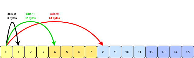
- Since each integer takes up 8 bytes of memory (we’re using the
int64dtype), the stride value for each dimension is 8 times the number of values that we need to jump. For instance, to move along axis 1, four values (32 bytes) are jumped, and to move along axis 0, eight values (64 bytes) need to be jumped. - When we write
a.transpose(1, 0, 2), we are swapping axes 0 and 1. The transposed array looks like this:
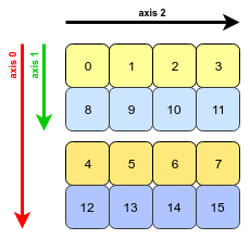
- All that NumPy needs to do is to swap the stride information for axis 0 and axis 1 (axis 2 is unchanged). Now we must jump further to move along axis 1 than axis 0:
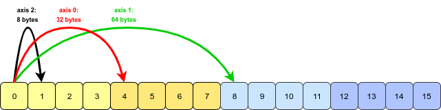
- This basic concept works for any permutation of an array’s axes. The actual code that handles the transpose is written in C and can be found here.
Reverse
- Reverse (or flip) the contents of an array along an axis.
- If
axisis not specified, it is assumedNone, which flips over all of the axes of the input array. - If axis is a tuple of ints, flipping is performed on all of the axes specified in the tuple.
import numpy as np

a = np.arange(8).reshape((2, 2, 2))

print(a)                  # Prints [[[0 1]
                          #          [2 3]]
                          #
                          #         [[4 5]
                          #          [6 7]]]

print(np.flip(a, 0))      # Prints [[[4 5]
                          #          [6 7]]
                          #
                          #         [[0 1]
                          #          [2 3]]]

print(np.flip(a, 1))      # Prints [[[2 3]
                          #          [0 1]]
                          #
                          #         [[6 7]
                          #          [4 5]]]

print(np.flip(a))         # Prints [[[7 6]
                          #          [5 4]]
                          #
                          #         [[3 2]
                          #          [1 0]]]

print(np.flip(a, (0, 2))) # Prints [[[5 4]
                          #          [7 6]]
                          #
                          #         [[1 0]
                          #          [3 2]]]
Flatten
- Return a copy of the array collapsed into one dimension.
import numpy as np

a = np.array([[1, 2, 3], [4, 5, 6]])
print(a.flatten()) # Prints [1 2 3 4 5 6]
Squeeze
- Remove single-dimensional axes from an input array.
- The “squeeze” nomenclature has been borrowed from MATLAB which removes axes of size one (singletons).
import numpy as np

a = np.array([[[0], [1], [2]]])

print(a.shape)             # Prints (1, 3, 1)
print(np.squeeze(a))       # Prints [0 1 2]
print(np.squeeze(a).shape) # Prints (3,)
print(a) # Prints [[[0]
         #          [1]
         #          [2]]]
- Note that unlike PyTorch, NumPy does not have offer an unsqueeze function, but similar functionality can be achieved using
np.newaxis.
Copy
- Return an array copy of the given object.
import numpy as np

a = np.array([[1, 2], [3, 4]])
b = a
c = np.copy(a)

a[0] = 10

print(a)     # Prints [[10 10]
             #         [ 3  4]]

a[0] == b[0] # Prints True
a[0] == c[0] # Prints False
- Note that
np.copy()performs a shallow copy and will not copy object elements within arrays. This is mainly important for arrays containing Python objects.
Element-wise sign
- Returns an element-wise sign of an array’s elements.
import numpy as np

a = np.array([[1, 2], [-3, -4]])

print(np.sign(a)) # Prints [[ 1  1]
                  #         [-1 -1]]
Sum
- Sum of an array’s elements.
import numpy as np

a = np.array([[1, 2], [3, 4]])

# Compute sum of each column
print(np.sum(a, axis=0)) # Prints [4 6]

# Compute sum of each row
print(np.sum(a, axis=1)) # Prints [3 7]
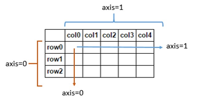
- The
axisargument specifies the axis along which the sum is performed. If axis is a tuple of ints, a sum is performed on all of the axes specified in the tuple instead of a single axis or all the axes as before. - Note that
np.sum()yields an array with the same shape as the original array with the specified axis removed (which implies that if you sum over the rows in a 2D matrix, you get as many entries in the output as the number of columns and vice versa). - In the above example, since
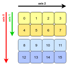
axis=0refers to the rows of the input matrix,np.sum()sums over all rows and in other words, computes the sum of each column. - As a visual description here’s how
np.sum()works under the hood (the arrows indicate the flow of summation foraxis=0oraxis=1):
- If
axisisn’t specified, it defaults toNone, in which casenp.sum()sums over all of the elements of the input array:
import numpy as np

a = np.array([[1, 2], [3, 4]])

# Compute sum of all elements
print(np.sum(a)) # Prints 10
- Some examples of
np.sum():
a = np.array([[1, 0], [0, 1]])

# Count number of 1s in the input array
print(np.sum(a)) # Prints 2

b = np.array([[1, 2], [2, 1]])

# Count number of 1s in the input array
print(np.sum(b == 1)) # Prints 2
Average/Mean
- Recall that the mean is the sum of the elements divided by the length of the vector.
import numpy as np

a = np.array([[1, -1], [2, -2], [3, -3]]) # Define a 3x2 matrix. Chosen to be a matrix with 0 mean.

# Get the mean for the whole matrix
print(np.mean(a)) # Prints 0.0

# Get the mean for each column. Returns 2 elements.
print(a, axis=0)  # Prints [ 2. -2.]

# Get the mean for each row. Returns 3 elements.
print(a, axis=1)  # Prints [0. 0. 0.]
Product
- Return the product of array elements over a given axis.
import numpy as np

a = np.array([[1, 2], [3, 4]])

print(np.prod(a)) # Prints 24
Len
len()returns the size of the first dimension of the input tensor, similar to PyTorch.
import numpy as np

a = np.array([[1, 2], [3, 4]])
print(a) # Prints [[1, 2],
         #         [3, 4]]
len(a)   # 2

b = np.array([1, 2, 3, 4])
print(b) # Prints [1 2 3 4]
len(b)   # 4
Dot Product
- Refer to the earlier section on dot product to learn the usage of
np.dot(). Note that the dot product (also called the inner/scalar product) yields a scalar.
Outer Product
- Return the outer product of two vectors. Note that the outer product yields a vector.
import numpy as np

a = np.ones((5,))
b = np.linspace(-2, 2, 5)

print(np.outer(a, b))
# Prints:
# [[-2. -1.  0.  1.  2.]
#  [-2. -1.  0.  1.  2.]
#  [-2. -1.  0.  1.  2.]
#  [-2. -1.  0.  1.  2.]
#  [-2. -1.  0.  1.  2.]]
Matrix Product
- Return matrix product of two arrays.
- The following rules dictate the behavior of
np.matmul()depending on the arguments:- If both arguments are 2D, they are multiplied like conventional matrices.
- If either argument is N-dimensional (with \(N > 2\)), it is treated as a stack of matrices residing in the last two indexes and broadcast accordingly.
- If the first argument is 1D (while the second is N-dimensional, where \(N \geq 2\)), it is promoted to a matrix by prepending a 1 to its dimensions. After matrix multiplication, the prepended 1 is removed.
- If the second argument is 1D (while the second is N-dimensional, where \(N \geq 2\)), it is promoted to a matrix by appending a 1 to its dimensions. After matrix multiplication, the appended 1 is removed.
import numpy as np

# For 2D arrays, np.matmul() is the conventional matrix product.
a = np.array([[1, 0], [0, 1]])
b = np.array([[4, 1], [2, 2]])

print(np.matmul(a, b)) # Prints [[4 1]
                       #         [2 2]]

# For 2D mixed with 1D, the result is the usual., np.matmul() is the conventional matrix product.
a = np.array([[1, 0], [0, 1]])
b = np.array([1, 2])

# The output matrices below are both 1D after the removal of the appended/prepended 1 dimension
print(np.matmul(a, b)) # Prints [1 2]
print(np.matmul(b, a)) # Prints [1 2]
np.matmul() vs. np.dot()
np.matmul()differs fromnp.dot()in two important ways:- Multiplication by scalars is not allowed, use
*instead. - Stacks of matrices (i.e., tensors) are broadcast together as if the matrices were elements, respecting the signature \((n, k) \times (k, m) \rightarrow (n, m)\):
- Multiplication by scalars is not allowed, use
import numpy as np

a = np.ones([9, 5, 7, 4])
c = np.ones([9, 5, 4, 3])
print(np.dot(a, c).shape)    # Prints (9, 5, 7, 9, 5, 3)
print(np.matmul(a, c).shape) # Prints (9, 5, 7, 3) / n is 7, k is 4, m is 3 per the stacked-matrices rule
Max
- Return the maximum element of an array or maximum along an axis.
import numpy as np

a = np.array([[1, 2, 3], [4, 5, 6]])

print(np.max(a)) # Prints 6
Element-wise max
- Compare two compatible arrays and return their element-wise maximum. Here, ‘compatible’ means that one array can be broadcast to the other.
import numpy as np

a = np.array([[1, 2, 3], [4, 5, 6]])
b = np.array([[7, 8, 9], [-2, -1, 0]])

print(np.maximum(a, b)) # Prints [[7 8 9]
                        #         [4 5 6]]
Argmax
- Return the indices of the maximum values along an axis.
import numpy as np

a = np.array([[1, 2, 3], [4, 5, 6]])

print(np.argmax(a))         # Prints 5
print(np.argmax(a, axis=0)) # Prints [1 1 1]
print(np.argmax(a, axis=1)) # Prints [2 2]
- Note that in case of multiple occurrences of the maximum values, only the index corresponding to the first occurrence is returned.
Argmin
- Return the indices of the minimum values along an axis.
import numpy as np

a = np.array([[1, 2, 3], [4, 5, 6]])

print(np.argmin(a))         # Prints 0
print(np.argmin(a, axis=0)) # Prints [0 0 0]
print(np.argmin(a, axis=1)) # Prints [0 0]
- Note that in case of multiple occurrences of the minimum values, only the index corresponding to the first occurrence is returned.
Where
np.where()accepts three arguments:(condition, x, y). If only theconditionargument is supplied,np.where()simply returns the indicies of the elements in the input array which satisfy the condition:
a = np.array([[1, 0], [0, 1]])

print(np.where(c == 1)) # Print (array([0, 1]), array([0, 1]))
- If all three arguments are supplied, it first evaluates the
conditionargument – if it returnsTrue, it returnsx, otherwise yieldsy.
import numpy as np

a = np.array([0, 1, 2, 3, 4, 5])

print(np.where(a < 3, a, 10*a)) # Prints [ 0  1  2 30 40 50]
Pad
- Pad an array.
np.pad()accepts three arguments:array, pad_width, mode='constant'.pad_widthspecifies the number of values padded to the edges of each axis. It accepts both an int and a tuple.(pad,)or simply apad(as an int) is a shortcut for before = after = pad width for all axes.((before_1, after_1), ... (before_N, after_N))specifies the padding widths for each axis.((before, after),)yields same before and after padding width for each axis.
- When
modeis set toconstant(which is the default), an optional parameterconstant_valueslet’s you specify the padding values for each axis, which has a default of0(i.e., zero padding). Rather than just an int,constant_valuesaccepts a tuple as well:(constant,)or simply aconstant(as an int) is a shortcut forbefore = after = constantfor all axes. Default is0.((before_1, after_1), ... (before_N, after_N))specifies the unique pad constants for each axis.((before, after),)yields same before and after constants for each axis.
import numpy as np

a = np.array([1, 2, 3, 4, 5])
print(np.pad(a, 1, 'constant'))                              # Prints [0 1 2 3 4 5 0]
print(np.pad(a, (2, 3), 'constant', constant_values=(4, 6))) # Prints [4 4 1 2 3 4 5 6 6 6]

a = np.array([[1, 2], [3, 4]])
print(np.pad(a, 1, 'constant', constant_values=(4, 6)))      # Prints [[4 4 4 6]
                                                             #         [4 1 2 6]
                                                             #         [4 3 4 6]
                                                             #         [4 6 6 6]]

# With pad_width = [(0, 1), (0, 1)], each tuple item in the pad_width list
# corresponds to a dimension and the item therein represents the padding
# before (first element) and after (second element). Graphically,
# [(0, 1), (0, 1)]
#          ^^^^^^------ padding for second dimension
#  ^^^^^^-------------- padding for first dimension
#
#   ^------------------ no padding at the beginning of the first axis
#      ^--------------- pad with one "value" at the end of the first axis.
a = np.ones(2, 2)
print(np.pad(a, [(0, 1), (0, 1)], mode='constant'))          # Prints [[1 2 0]
                                                             #         [3 4 0]
                                                             #         [0 0 0]]

# In this case the padding for the first and second axis are identical,
# so one could also just pass in the 2-tuple.
print(np.pad(a, (0, 1), mode='constant'))                    # Prints [[1 2 0]
                                                             #         [3 4 0]
                                                             #         [0 0 0]]

# In case the padding before and after is identical, one could even omit
# the tuple (not applicable in this case though):
print(np.pad(a, 1, mode='constant'))                         # Prints [[0 0 0 0]
                                                             #         [0 1 2 0]
                                                             #         [0 3 4 0]
                                                             #         [0 0 0 0]]

# Or if the padding before and after is identical but different for the axis, you could also omit the second argument in the inner tuples:
print(np.pad(a, [(1, ), (2, )], mode='constant'))            # Prints [[0 0 0 0 0 0]
                                                             #         [0 0 1 2 0 0]
                                                             #         [0 0 3 4 0 0]
                                                             #         [0 0 0 0 0 0]]
- However using the explicit
pad_widthspecification should be preferred because it’s just to easy to make mistakes, as in the case below:
# Here NumPy thinks you wanted to pad all axis with 1 element before and
# 2 elements after each axis!
# Even if you intended it to pad with 1 element in axis 1 and 2 elements for axis 2.
print(np.pad(a, [1, 2], mode='constant')) # Prints [[0 0 0 0 0]
                                          #         [0 1 2 0 0]
                                          #         [0 3 4 0 0]
                                          #         [0 0 0 0 0]
                                          #         [0 0 0 0 0]]
Ravel
- Return a contiguous flattened array.
- Note that
np.ravel()returns a view of the array when the elements are contiguous in memory (just likenp.reshape()). So modifying the result ofnp.ravel()would also modify the original array. However,np.ravel()returns a copy if, say the input array were made from slicing another array using a non-unit step size (for e.g.,a = x[::2]).
import numpy as np

a = np.array([[1, 2, 3], [4, 5, 6]])
print(np.ravel(a)) # Prints [1 2 3 4 5 6]
- Note that
np.ravel()is equivalent tonp.reshape(-1).
import numpy as np

a = np.array([[1, 2, 3], [4, 5, 6]])
print(np.reshape(a, -1)) # Prints [1 2 3 4 5 6])
Unravel Index
- Converts a “flat” index (i.e., an index into the flattened version of an array) into a tuple of coordinate arrays.
import numpy as np

# Passing an integer array whose elements are indices into the flattened version of an array
print(np.unravel_index([1, 2, 3], [4, 5])) # Prints (array([0, 0, 0]), array([1, 2, 3]))

# You're not limited to the 2-dimensional XY co-ordinate space
print(np.unravel_index(7, (1, 1, 7)))     # Prints (0, 0, 6)
Internals
- Computer memory is addressed linearly. Each memory cell corresponds to a number. A block of memory can be addressed in terms of a base, which is the memory address of its first element, and the item index. For example, assuming the base address is 10,000:
item index      0       1       2       3
memory address  10,000  10,001  10,002  10,003
- To store multi-dimensional blocks, their geometry must somehow be made to fit into linear memory. In C and NumPy, this is done row-by-row (which is known as the row-major order). A 2D example would be:
     | 0      1      2      3
   --+------------------------
   0 | 0      1      2      3
   1 | 4      5      6      7
   2 | 8      9     10     11
- So, for example, in this 3-by-4 block the 2D index \((1, 2)\) would correspond to the linear index 6 which is \(1 \times 4 + 2\). In general, the linear index is given by: \(\text{row index }\times\text{row length }+\text{ column index}\).
np.unravel_index()does the inverse. Given a linear index, it computes the corresponding coordinates. Since this depends on the block dimensions, these also have to be passed. So, in our example, we can get the original 2D index \((1, 2)\) back from the linear index 6:np.unravel_index(6, (3, 4))) # Prints (1, 2)
Exponential
- Calculate the exponential of all elements in the input array.
import numpy as np

a = np.array([[1, 2, 3], [4, 5, 6]])

print(np.exp(a)) # Prints [[   2.71828183    7.3890561    20.08553692]
                 #         [  54.59815003  148.4131591   403.42879349]]
Unique
- Find the unique elements of an array.
import numpy as np

a = np.array([[1, 1, 1], [2, 2, 2]])

print(np.unique(a)) # Prints [1 2]
np.unique()supports an optionalreturn_indexargument which returns the indices with unique elements in addition to the unique elements.
import numpy as np

a = np.array([[1, 1, 1], [2, 2, 2]])

unique_els, indices = np.unique(a, return_index=True)
unique_els # Prints array([1, 2])
indices    # Prints array([0, 3])
np.unique()also supports an optionalreturn_countsargument which returns the counts corresponding to the unique elements in addition to the unique elements.
import numpy as np

a = np.array([[1, 1, 1], [2, 2, 2]])

unique_els, counts = np.unique(a, return_counts=True)
unique_els # Prints array([1, 2])
counts     # Prints array([3, 3])
Bincount
- Count number of occurrences of each value in a one-dimensional array of non-negative integers.
import numpy as np

a = np.array([1, 1, 1, 2, 2, 2])

print(np.bincount(a)) # Prints [0 3 3]
Element-wise square
- Return the element-wise square of the input.
import numpy as np

a = np.array([[1, 2, 3], [4, 5, 6]])

print(np.square(a)) # Prints [[ 1   4  9]
                    #         [[16 25 36]]
Element-wise square root
- Return the element-wise non-negative square root of an array.
import numpy as np

a = np.array([[1, 4, 9], [16, 25, 36]])

print(np.sqrt(a)) # Prints [[1. 2. 3.]
                  #         [4. 5. 6.]]
Split
- Split an array into multiple sub-arrays.
import numpy as np

a = np.arange(8)

print(np.split(a, 2)) # Prints [array([0, 1, 2, 3]), array([4, 5, 6, 7])]
Swapaxes
- Interchange two axes of an array.
import numpy as np

a = np.zeros((2, 3, 5))
print(a.shape)                     # Prints (2, 3, 5)

print(np.swapaxes(a, 0, -1).shape) # Prints (5, 3, 2)
Moveaxis
- Compared to
np.transpose()for reordering axes which needs positions of all axes to be explicitly specified, moving one axis while keeping the relative positions of all others is a common enough use-case to warrant its own syntactic sugar. This is the functionality that is offered bynp.moveaxis().
import numpy as np

a = np.zeros((2, 3, 5))
print(a.shape)                     # Prints (2, 3, 5)

print(np.moveaxis(a, 0, -1).shape) # Prints (3, 5, 2)
Horizontal split
- Split an array into multiple sub-arrays horizontally (column-wise).
- Note that
np.hsplit()is equivalent tonp.splitwithaxis=1. Put simply, withnp.hsplit(), the array is always split along the second axis regardless of the array dimension.
import numpy as np

a = np.arange(4).reshape(2, 2)

print(a)               # Prints [[0 1]
                       #         [2 3]]

print(np.hsplit(a, 2)) # Prints [array([[0],
                       #                [2]]),
                       #        [array([[1],
                       #                [3]])]
Vertical split
- Split an array into multiple sub-arrays vertically (row-wise).
- Note that
np.vsplit()is equivalent tonp.splitwithaxis=0(which is the default fornp.split). Put simply, withnp.vsplit(), the array is always split along the second axis regardless of the array dimension.
import numpy as np

a = np.arange(4).reshape(2, 2)

print(a)               # Prints [[0 1]
                       #         [2 3]]

print(np.vsplit(a, 2)) # Prints [array([[0, 1]]), array([[2, 3]])]

# np.split() with axis=0 (which is the defauly) yields the same output as np.vsplit()
print(np.split(a, 2))  # Prints [array([[0, 1]]), array([[2, 3]])]
Append
- Append values to the end of an array. If the
axisargument is not given, both the input array and values are flattened before use.
import numpy as np

a = np.array([[1, 2, 3], [4, 5, 6]])
b = np.array([[7, 8, 9]])

print(np.append(a, b))         # Prints [1 2 3 4 5 6 7 8 9]
print(np.append(a, b, axis=0)) # Prints [[1 2 3]
                               #         [4 5 6]
                               #         [7 8 9]]
- As another example:
a = np.arange(4).reshape(2, 2) # Prints [[0 1]
                               #         [2 3]]
print(np.append(a, a))         # Prints [0 1 2 3 0 1 2 3]
print(np.append(a, a, axis=0)) # Prints [[0 1]
                               #         [2 3]
                               #         [0 1]
                               #         [2 3]]
- With
np.append(), it is important to note that both input arrays must have the same shape. However, ifaxisis not specified, the input arrays can be any shape (since they will be flattened before use).
import numpy as np

a = np.array([[1, 2, 3], [4, 5, 6]])
b = np.array([7, 8, 9])

print(np.append(a, b, axis=0)) # ValueError: all the input arrays must have same number of dimensions
print(np.append(a, b))         # Prints [1 2 3 4 5 6 7 8 9]
Stack
- Join a sequence of arrays along a new axis.
- The
axisparameter specifies the index of the new axis in the dimensions of the result. For e.g.,axis=0denotes the first dimension andaxis=-1denotes the last dimension. Note that by default,axisis set to 0.
import numpy as np

a = np.array([1, 2, 3])
b = np.array([4, 5, 6])

print((a, b))                   # Prints (array([1, 2, 3]), array([4, 5, 6]))

print(np.stack((a, b)))         # Prints [[1 2 3]
                                #         [4 5 6]]

# This is the same as above since axis is set to 0 by default
print(np.stack((a, b), axis=0)) # Prints [[1 2 3]
                                #         [4 5 6]]
- For the given input arrays
aandb, note thatnp.vstack()command yields the same output asnp.stack(), sincenp.vstack()simply stacks them vertically (row-wise) thereby implicitly creating a new dimension (since the input arrays are 1D and cannot be stacked without adding a dimension), whilenp.stack()adds a new dimension at index 0 explicitly and stacks them along that dimension.
import numpy as np

a = np.array([1, 2, 3])
b = np.array([4, 5, 6])

# This is the same as above since axis is set to 0 by default
print(np.stack((a, b), axis=0)) # Prints [[1 2 3]
                                #         [4 5 6]]

# np.vstack() yields the same output as np.stack()
# Note that np.vstack() is discussed in more detail below
print(np.vstack((a, b)))        # Prints [[1 2 3]
                                #         [4 5 6]]
- For the given input arrays
aandb, note thatnp.vstack()yields an output dissimilar tonp.stack(), sincenp.vstack()simply stacks them vertically (row-wise), whilenp.stack()adds a new dimension at index 0 explicitly and stacks them along that dimension.
import numpy as np

a = np.array([[1, 2], [3, 4]])
b = np.array([[5, 6], [7, 8]])

c = np.stack((a, b))
print(c)       # Prints [[[1 2]
               #          [3 4]]
               #
               #         [[5 6]
               #          [7 8]]]
print(c.shape) # Prints (2, 2, 2)

d = np.vstack((a, b))
print(d)       # Prints [[1 2]
               #         [3 4]
               #         [5 6]
               #         [7 8]]
print(d.shape) # Prints (4, 2)
- Joining arrays column-wise by doing horizontal stacking:
import numpy as np

a = np.array([1, 2, 3])
b = np.array([4, 5, 6])

print(np.stack((a, b), axis=1)) # Prints [[1 4]
                                #         [2 5]
                                #         [3 6]]

# Note np.hstack() does *not* match the output of np.stack()
print(np.hstack((a, b)))        # Prints [1 2 3 4 5 6]
- With
np.stack(), it is important to note that all input arrays must have exactly the same shape. Specifically, not only do the input arrays need to have the same number of dimensions (i.e., equal ranks), but also all the dimensions themselves should be equal-length. This is an important point of differentiation compared tonp.vstack()andnp.hstack()(which require only the concatenation axis to be equal-length).
import numpy as np

a = np.array([[[1, 2]]])
b = np.array([[3, 4]])

print(np.stack((a, b)))  # ValueError: all input arrays must have the same shape

a = np.array([[1, 2], [3, 4]])
b = np.array([[5, 6]])

print(np.stack((a, b)))  # ValueError: all input arrays must have the same shape
print(np.vstack((a, b))) # Prints [[1 2]
                         #         [3 4]
                         #         [5 6]]
- For arrays of rank \(\geq 2\) (i.e., tensors),
np.stack()works well too:
import numpy as np

arrays = [np.random.randn(3, 4) for _ in range(10)]
np.stack(arrays, axis=0).shape # Prints (10, 3, 4)
np.stack(arrays, axis=1).shape # Prints (3, 10, 4)
np.stack(arrays, axis=2).shape # Prints (3, 4, 10)
Vertical stack
- Stack arrays in sequence vertically (row-wise for 2D arrays). In general, for arrays of rank \(\geq 2\) (i.e., tensors), stack arrays along the first dimension.
- Note that
np.vstack()does not accept anaxisargument. np.vstack()is equivalent tonp.concatenate(<ndarray>, axis=0)along the first axis (after 1D arrays of shape(N,)have been reshaped to(1, N)).
import numpy as np

a = np.array([1, 2, 3])
b = np.array([4, 5, 6])

print(np.vstack((a, b))) # Prints [[1 2 3]
                         #         [4 5 6]]

a = np.array([[1], [2], [3]])
b = np.array([[4], [5], [6]])

print(np.vstack((a, b))) # Prints [[1]
                         #         [2]
                         #         [3]
                         #         [4]
                         #         [5]
                         #         [6]]
- With
np.vstack(), it is important to note that all input arrays must have:- The same number of dimensions (i.e., equal ranks), and
- Equal-length concatenation axes (in the case of 2D arrays, their respective second dimensions must be equal-length, i.e., the same number of columns). This is an important point of differentiation compared to
np.stack()andnp.hstack().
a = np.array([[1, 2], [3, 4]])
b = np.array([[5, 6]])

print(np.vstack((a, b))) # Prints [[1 2]
                         #         [3 4]
                         #         [5 6]]

a = np.array([[[1, 2]]])
b = np.array([[3, 4]])

print(np.vstack((a, b))) # ValueError: all the input arrays must have same number of dimensions

a = np.array([1, 2, 3])
b = np.array([4, 5])

print(np.vstack((a, b))) # ValueError: all the input array dimensions for the concatenation axis must match exactly
- For arrays of rank \(\geq 2\) (i.e., tensors),
np.vstack()works well too:
a = np.array([[[1, 2]]])
b = np.array([[[3, 4]]])
print(a.shape) # Prints (1, 1, 2)

c = np.vstack((a, b))
print(c)       # Prints [[[1 2]]
               #         [[3 4]]]

print(c.shape) # Prints (2, 1, 2)
Horizontal stack
- Stack arrays in sequence horizontally (column-wise for 2D arrays). In general, for arrays of rank \(\geq 2\) (i.e., tensors), stack arrays along the second dimension.
- Note that
np.hstack()does not accept anaxisargument. np.hstack()is equivalent tonp.concatenate(<ndarray>, axis=1), except for 1D arrays where it concatenates along the first axis.
import numpy as np

a = np.array([1, 2, 3])
b = np.array([4, 5, 6])

print(np.hstack((a, b))) # Prints [1 2 3 4 5 6]

a = np.array([[1], [2], [3]])
b = np.array([[4], [5], [6]])

print(np.hstack((a, b))) # Prints [[1 4]
                         #         [2 5]
                         #         [3 6]]
- With
np.hstack(), it is important to note that all input arrays must have:- The same number of dimensions (i.e., equal ranks), and
- Equal-length concatenation axes (in the case of 2D arrays, their respective first dimensions must be equal-length, i.e., the same number of rows). This is an important point of differentiation compared to
np.stack()andnp.vstack().
a = np.array([1, 2, 3])
b = np.array([4, 5])

print(np.hstack((a, b))) # Prints [1 2 3 4 5]

a = np.array([[[1, 2]]])
b = np.array([[3, 4]])

print(np.hstack((a, b))) # ValueError: all the input arrays must have same number of dimensions

a = np.array([[1, 2], [3, 4]])
b = np.array([[5, 6]])

print(np.hstack((a, b))) # ValueError: all the input array dimensions for the concatenation axis must match exactly
- For arrays of rank \(\geq 2\) (i.e., tensors),
np.hstack()works well too:
a = np.array([[[1, 2]]])
b = np.array([[[3, 4]]])
print(a.shape) # Prints (1, 1, 2)

c = np.hstack((a, b))
print(c)       # Prints [[[1 2]
               #          [3 4]]]

print(c.shape) # Prints (1, 2, 2)
Column Stack
- Take a sequence of 1D arrays and stack them as columns to make a single 2D array. 2D arrays are stacked as-is, just like with
np.hstack. 1D arrays are turned into 2D column vectors first.
import numpy as np

a = np.array([1, 2, 3])
b = np.array([4, 5, 6])

print(np.column_stack((a, b)))                       # Prints [[1 4]
                                                     #         [2 5]
                                                     #         [3 6]]

# The following np.stack() and np.hstack() commands
# return the same output as well
print(np.stack((a, b), axis=1))                      # Prints [[1 4]
                                                     #         [2 5]
                                                     #         [3 6]]
print(np.hstack(([[1], [2], [3]], [[4], [5], [6]]))) # Prints [[1 4]
                                                     #         [2 5]
                                                     #         [3 6]]
- Note that
np.column_stack()is equivalent tonp.vstack().T:
import numpy as np

a = np.array([1, 2, 3])
b = np.array([4, 5, 6])

# np.vstack().T returns the same output as np.column_stack()
print(np.vstack((a, b)).T) # Prints [[1 4]
                           #         [2 5]
                           #         [3 6]]
Concatenate
- Join a sequence of arrays along an existing axis.
- The
axisargument specifies the axis along which the arrays will be joined. If axis isNone, the arrays are flattened before use. The default is0(vertical/row-wise stacking). - Joining arrays row-wise by doing vertical stacking:
import numpy as np

a = np.array([[1, 2], [3, 4]])
b = np.array([[5, 6]])

print(np.concatenate((a, b)))         # Prints [[1 2]
                                      #         [3 4]
                                      #         [5 6]]

# The following np.vstack() command returns the same output
print(np.vstack((a, b)))              # Prints [[1 2]
                                      #         [3 4]
                                      #         [5 6]]
- Joining arrays column-wise by doing horizontal stacking:
print(np.concatenate((a, b.T), axis=1)) # Prints [[1 2 5]
                                        #         [3 4 6]]

# The following np.hstack() and np.column_stack() command
# return the same output as well
print(np.hstack((a, b.T)))              # Prints [[1 2 5]
                                        #         [3 4 6]]

print(np.column_stack((a, b.T)))        # Prints [[1 2 5]
                                        #         [3 4 6]]
- Joining arrays after flattening them:
print(np.concatenate((a, b), axis=None)) # Prints [1 2 3 4 5 6]

# The following np.append() command returns the same output as well
print(np.append(a, b))                   # Prints [1 2 3 4 5 6]
Concatenate vs. hstack/vstack vs. append vs. column_stack
- All the aforementioned functions, except
np.concatenate(), are written in Python and work by tweaking the dimensions of the input arrays, and then concatenating on the right axis. In other words, they are convenience functions since they’re just wrappers aroundnp.concatenate(). Here’s a summary of their code:
vstack:
# Turn all inputs into 2D (or more) and concatenate on first dimension
concatenate([atleast_2d(_m) for _m in tup], axis=0)
# Equivalent to np.concatenate(tup, axis=0) if input tuple contains arrays that are at least 2D

hstack:
concatenate([atleast_1d(_m) for _m in tup], axis=<0 or 1>)

column_stack:
if needed, transform arrays using array(arr, copy=False, subok=True, ndmin=2).T
concatenate([atleast_1d(_m) for _m in tup], axis=1)

append:
concatenate((asarray(arr), values), axis=axis)
- As a side note, with an IPython shell you can use
??to query the source code of a particular function.
Graphical treatment
- If you have two matrices,
np.hstack()stacks horizontally whilenp.vstack()stacks vertically:
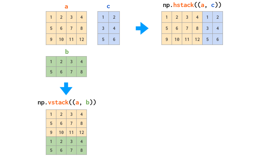
- If you’re stacking a matrix and a vector,
np.hstack()becomes tricky to use, sonp.column_stack()is a better option. The problem withnp.hstack()is that when you append a column, you need convert it from a 1D array to a 2D column vector first, because a 1D array is normally interpreted as a row vector in 2D context in NumPy:
a = np.ones(2)       # 2D, shape = (2, 2)
b = np.array([0, 0]) # 1D, shape = (2,)

np.hstack((a, b))    # Dimensions mismatch error
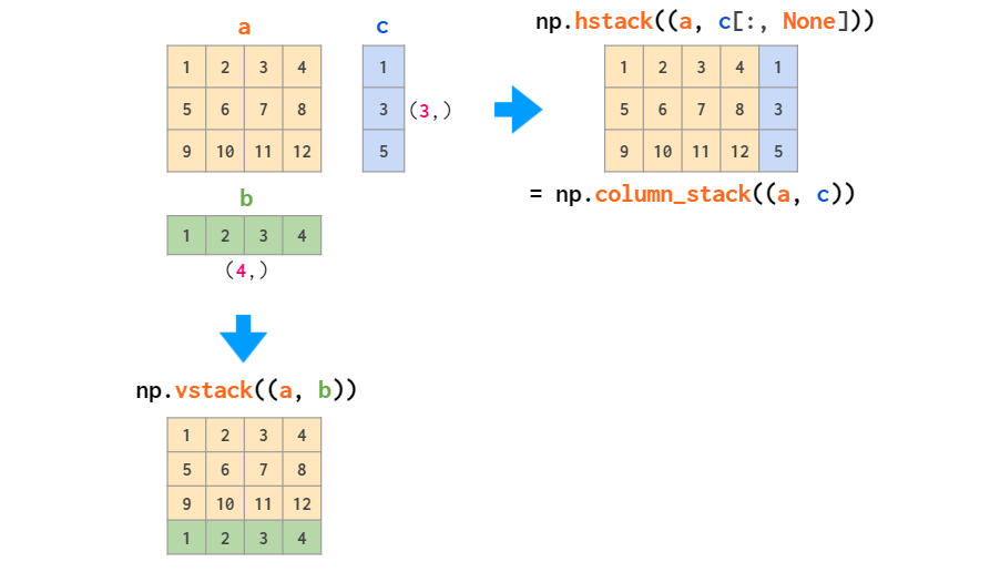
- If you’re stacking two vectors, you’ve got three options:
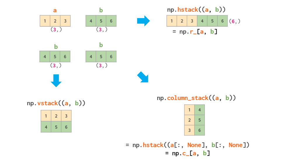
np.concatenate()in its raw form is useful for 3D arrays and above (i.e., tensors).
New axis
np.newaxisis used to increase the dimension of the existing array by an additional dimension, for e.g., a 1D array gets transformed to a 2D array, a 2D array gets transformed to a 3D array, and so on.- Essentially,
np.newaxisis a pseudo-index that allows the temporary addition of an axis into a multiarray. - Here is a visual illustration which depicts the promotion of a 1D array to a 2D array (row/column vector):
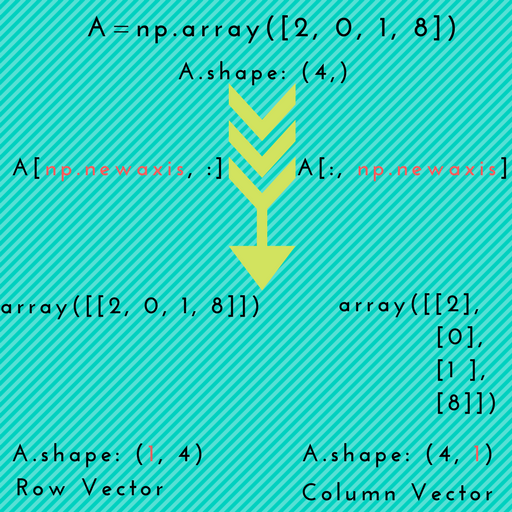
Usecase: 1D array -> 2D vector
np.newaxismight come in handy when you wish to explicitly convert a 1D array to either a 2D row or a column vector, as depicted in the above picture. The section on Transpose also describes this usecase. As an example:
# Define a 1D array
a = np.arange(4)
a.shape                    # Prints (4,)

# Make "a" a row vector by inserting an axis along the first dimension
row_vec = a[np.newaxis, :] # or a[None, :]
row_vec.shape              # Prints (1, 4)

# Make "a" a column vector by inserting an axis along the second dimension
col_vec = a[:, np.newaxis] # or arr[:, None]
col_vec.shape              # Prints (4, 1)
Usecase: During broadcasting
- When making use of broadcasting as part of some operation, for instance while doing addition of some arrays,
np.newaxisproves useful by inserting a new dimension with size 1 (which is one of the required conditions for broadcasting to work). As an example, let’s say you want to add the following two arrays:
import numpy as np

a = np.array([1, 2, 3, 4, 5])
b = np.array([5, 4, 3])
- If you try to add these 1D arrays just like that, NumPy will raise the following
ValueError:
# ValueError: operands could not be broadcast together with shapes (5,) (3,)
- To remedy this, you can use
np.newaxisto increase the dimension of one of the arrays so that NumPy can broadcast:
# Let's utilize np.newaxis with a
a_new = a[:, np.newaxis] # or a[:, None]
a_new.shape              # Prints (5, 1)
print(a_new)             # Prints [[1]
                         #         [2]
                         #         [3]
                         #         [4]
                         #         [5]]

# Now, add
print(a_new + b)         # Prints [[ 6  5  4]
                         #         [ 7  6  5]
                         #         [ 8  7  6]
                         #         [ 9  8  7]
                         #         [10  9  8]]

# Alternatively, you can also utilize np.newaxis with b
b_new = b[:, np.newaxis] # or b[:, None]
b_new.shape              # Prints (3, 1)
print(b_new)             # Prints [[5]
                         #         [4]
                         #         [3]]

# Now, add
print(a + b_new)         # Prints [[ 6  7  8  9 10]
                         #         [ 5  6  7  8  9]
                         #         [ 4  5  6  7  8]]

# Note that we get the same result in both cases (but one being the transpose of the other)
- In the example below, we inserted a temporary axis using
np.newaxisbetween the first and second axes of B to enable broadcasting.
import numpy as np

a = np.ones((3, 4, 5, 6))
b = np.ones((4, 6))

print((a + b[:, np.newaxis, :]).shape) # Prints (3, 4, 5, 6)
# or b[:, None, :]
Usecase: Promote to higher dimensions
- This is similar to Usecase: 1D array -> 2D vector with the only exception being that this usecase involves repeated use of
np.newaxismore than once to promote the input array to higher dimensions. Such an operation is sometimes needed for higher order arrays (i.e. Tensors).
import numpy as np

a = np.arange(5*5).reshape(5,5)
a.shape      # Prints (5, 5)

# Promoting 2D array to a 5D array
arr_5D = a[np.newaxis, ..., np.newaxis, np.newaxis] # or a[None, :, None, None]

arr_5D.shape # Prints (1, 5, 5, 1, 1)
np.newaxis vs. np.reshape()
np.newaxisuses the slicing operator to recreate the array whilenp.reshape()reshapes the array to the desired layout (assuming that the dimensions match; which is a must for a reshape to happen).- Using
np.reshape(), we can achieve a similar end result as withnp.newaxis:
import numpy as np

a = np.array([1, 2, 3])
print(a.shape)                              # Print (3,)
# Transform the 1D array to a row vector by reshaping with (1, -1), i.e., 1 row and 3 columns
print(a.reshape(1, -1).shape)               # Prints (1, 3)

a = np.array([1, 2, 3])
# Both of the np.newaxis commands yield the same output
print(a[np.newaxis, ...].shape)             # Prints (1, 3)
print(a[np.newaxis, :].shape)               # Prints (1, 3)

a = np.array([1, 2, 3])
# Transform the 1D array to a column vector by reshaping with (-1, 1), i.e., 3 rows and 1 column
print(a.reshape(-1, 1).shape)               # Prints (3, 1)

a = np.array([1, 2, 3])
# Both of the np.newaxis commands yield the same output
print(a[..., np.newaxis].shape)             # Prints (3, 1)
print(a[:, np.newaxis].shape)               # Prints (3, 1)

b = np.array([[1, 2, 3], [4, 5, 6]])
print(b.shape)                              # Print (2, 3)
# Transform the input array to dimensions (1, 2, 3, 1)
print(b.reshape(1, 2, 3, 1).shape)          # Prints (1, 2, 3, 1)

b = np.array([[1, 2, 3], [4, 5, 6]])
# Transform the input array to dimensions (1, 2, 3, 1)
print(b[np.newaxis, ..., np.newaxis].shape) # Prints (1, 2, 3, 1)
None as a shortcut for np.newaxis
- You can also use
Nonein place ofnp.newaxis; these are in fact the same objects.
np.newaxis is None # Prints True
Expand dims
- As an alternative to
np.newaxis, you can usenp.expand_dims():
import numpy as np

a = np.arange(5*5).reshape(5,5)

# Use np.expand_dims to add an axis at index position 1
b = np.expand_dims(a, axis=1)
print(b.shape) # Prints (6, 1)

# Use np.expand_dims to add an axis at index position 0
c = np.expand_dims(a, axis=0)
print(c.shape) # Prints (1, 6)

# Using the intuitive `axis` argument to add new axes at the
# 1st, 4th, and last (-1) dimension of the resulting array
arr_5D = np.expand_dims(a, axis=(0, 3, -1))
arr_5D.shape   # Prints (1, 5, 5, 1, 1)
Inverse
- Compute the inverse of a matrix.
import numpy as np
from numpy.linalg import inv

a = np.array([[1., 2.], [3., 4.]])

print(inv(a)) # Prints [[-2.   1. ]
              #         [ 1.5 -0.5]]
Solve
- Solve a linear matrix equation, or system of linear scalar equations.
import numpy as np
from numpy.linalg import solve

# Solve the system of equations:
# x0 + 2 * x1 = 1
# 3 * x0 + 5 * x1 = 2
a = np.array([[1, 2], [3, 5]])
b = np.array([1, 2])

print(np.linalg.solve(a, b)) # Prints [-1.  1.]
Test any
- Test whether any array element along a given axis evaluates to
True. - Returns a single boolean unless
axisis notNone(which is the default). - Note that not a number (NaN), \(\infty\) and \(-\infty\) all evaluate to
Truebecause these are not equal to 0.
import numpy as np

a = [[True, False], [True, True]]
print(np.any(a))                         # Prints True

a = [[True, False], [True, True]]
print(np.any(a, axis=0))                 # Prints [ True, True]

a = np.array([[1, 2], [3, 4]])
print(np.any(a))                         # Prints True

# A nifty use-case of np.any() is to select elements that satisfy
# atleast one condition from multiple given conditions
a = np.array([[1, 2], [3, 4]])
print(np.any([a > 1, a < 5], axis=0))    # Prints [[ True  True]
                                         #         [ True  True]]
print(a[np.any([a > 1, a < 5], axis=0)]) # Prints [1 2 3 4]

# If axis is None (default), np.any() yields a single boolean by performing
# a logical OR reduction over all the dimensions of the input array
print(np.any([a > 1, a < 5]))            # Prints True
Test all
- Test whether all array elements along a given axis evaluate to
True. - Similar to
np.any(),np.all()returns a single boolean unlessaxisis notNone(which is the default). - Again, similar to
np.any(), note that not a number (NaN), \(\infty\) and \(-\infty\) all evaluate toTruebecause these are not equal to 0.
import numpy as np

a = [[True, False], [True, True]]
print(np.all(a))                         # Prints True

a = [[True, False], [True, True]]
print(np.all(a, axis=0))                 # Prints [ True, False]

a = np.array([[1, 2], [3, 4]])
print(np.all(a))                         # Prints True

# A nifty use-case of np.all() is to select elements that satisfy
# all given conditions
a = np.array([[1, 2], [3, 4]])
print(np.all([a > 1, a < 5], axis=0))    # Prints [[False  True]
                                         #         [ True  True]]
print(a[np.all([a > 1, a < 5], axis=0)]) # Prints [2 3 4]

# Note that if only one condition is specified, np.any() and np.all()
# are equivalent, and have identical outputs
print(a[np.any([a > 1], axis=0)])        # Prints [2 3 4]
print(a[np.all([a > 1], axis=0)])        # Prints [2 3 4]

# If axis is None (default), np.all() yields a single boolean by performing
# a logical AND reduction over all the dimensions of the input array
print(np.all([a > 1, a < 5]))            # Prints False
Convert NumPy Array to Python List
<ndarray>.tolist()returns the NumPy array as a nested list of Python scalars.
import numpy as np

a = np.arange(9).reshape(3, 3)

a.tolist() # Prints [[0, 1, 2], [3, 4, 5], [6, 7, 8]]
References
- Parts of this tutorial were originally contributed by Justin Johnson.
- Stanford CS231n Python/NumPy Tutorial served as a major inspiration for this tutorial.
- NumPy documentation: the absolute basics for beginners
- NumPy documentation: Broadcasting
- NumPy Illustrated: The Visual Guide to NumPy
- What is an intuitive explanation of np.unravel_index?
- When should I use hstack/vstack vs. append vs. concatenate vs. column_stack?
- What is the difference between NumPy’s array() and asarray() functions?
- What does -1 mean in NumPy reshape?
- Find the most frequent number in a NumPy vector
- NumPy: From ND to 1D arrays
- Difference between functions generating random numbers in NumPy
- How do I select elements of an array given condition?
- How does NumPy’s transpose() method permute the axes of an array?
- What is the difference between contiguous and non-contiguous arrays?
- When should I use hstack/vstack vs append vs concatenate vs column_stack?
- NumPy vstack vs. column_stack
- How does numpy.newaxis work and when to use it?
- What does numpy.concatenate do with a single argument?
- NumPy: Add new dimensions to ndarray (np.newaxis, np.expand_dims)
- How to pad NumPy array with zeros?
- NumPy: Slicing ndarray
Further Reading
Here are some (optional) link(s) you may find interesting:
Citation
If you found our work useful, please cite it as:
@article{Chadha2020NumPyPrimer,
  title   = {NumPy Primer},
  author  = {Chadha, Aman},
  journal = {Distilled AI},
  year    = {2020},
  note    = {\url{https://aman.ai}}
}