Natural Language Processing • Word Vectors/Embeddings
- Overview
- Motivation
- Word Embeddings
- Conceptual Framework of Word Embeddings
- Related: WordNet
- Background: Synonymy and Polysemy (Multi-Sense)
- Word Embedding Techniques
- Bag of Words (BoW)
- Term Frequency-Inverse Document Frequency (TF-IDF)
- Best Match 25 (BM25)
- Key Components of BM25
- Example
- BM25: Evolution of TF-IDF
- Limitations of BM25
- Parameter Sensitivity
- Non-Handling of Semantic Similarities
- Ineffectiveness with Short Queries or Documents
- Length Normalization Challenges
- Query Term Independence
- Difficulty with Rare Terms
- Performance in Specialized Domains
- Ignoring Document Quality
- Vulnerability to Keyword Stuffing
- Incompatibility with Complex Queries
- Word2Vec
- Motivation behind Word2Vec: The Need for Context-based Semantic Understanding
- Core Idea
- Word2Vec Architectures
- Training and Optimization
- Embedding and Semantic Relationships
- Distinction from Traditional Models
- Semantic Nature of Word2Vec Embeddings
- Key Limitations and Advances in Word2Vec and Word Embeddings
- Further Learning Resources
- Global Vectors for Word Representation (GloVe)
- fastText
- BERT Embeddings
- Handling Polysemous Words – Key Limitation of BoW, TF-IDF, BM25, Word2Vec, GloVe, and fastText
- Example: BoW, TF-IDF, BM25, Word2Vec, GloVe, fastText, and BERT Embeddings
- Summary: Types of Embeddings
- Comparative Analysis of BoW, TF-IDF, BM25, Word2Vec, GloVe, fastText, and BERT Embeddings
- FAQs
- Related: Matryoshka Representation Learning
- References
- Citation
Overview
- Word embeddings are a fascinating aspect of modern computational linguistics, particularly in the domain of Natural Language Processing (NLP). These embeddings serve as the foundation for interpreting and processing human language in a format that computers can understand and utilize. Here, we delve into an overview of word embeddings, focusing on their conceptual framework and practical applications.
Motivation
- J.R. Firth’s Insight and Distributional Semantics: The principle of distributional semantics is encapsulated in J.R. Firth’s famous quote (below), which highlights the significance of contextual information in determining word meaning and captures the importance of contextual information in defining word meanings. This principle is a cornerstone in the development of word embeddings.
“You shall know a word by the company it keeps.”
- Role in AI and NLP: Situated at the heart of AI, NLP aims to bridge the gap between human language and machine understanding. The primary motivation for developing word embeddings within NLP is to create a system where computers can not only recognize but also understand and interpret the subtleties and complexities of human language, thus enabling more natural and effective human-computer interactions.
- Advancements in NLP: The evolution of NLP, especially with the integration of deep learning methods, has led to significant enhancements in various language-related tasks, underscoring the importance of continuous innovation in this field.
- Historical Context and Evolution: With over 50 years of development, originating from linguistics, NLP has grown to embrace sophisticated models that generate word embeddings. The motivation for this evolution stems from the desire to more accurately capture and represent the nuances and complexities of human language in digital form.
- Word embeddings as a lens for nuanced language interpretation: Word embeddings, underpinned by the concept of distributional semantics, represent word meanings through vectors of real numbers. While not perfect, this method provides a remarkably effective means of interpreting and processing language in computational systems. The ongoing developments in this field continue to enhance our ability to model and understand natural language in a digital context.
Word Embeddings
- Word embeddings, also known as word vectors, provide a dense, continuous, and compact representation of words, encapsulating their semantic and syntactic attributes. They are essentially real-valued vectors, and the proximity of these vectors in a multidimensional space is indicative of the linguistic relationships between words.
An embedding is a point in an \(N\)-dimensional space, where \(N\) represents the number of dimensions of the embedding.
-
This concept is rooted in the Distributional Hypothesis, which posits that words appearing in similar contexts are likely to bear similar meanings. Consequently, in a high-dimensional vector space, vectors representing semantically related words (e.g., ‘apple’ and ‘orange’, both fruits) are positioned closer to each other compared to those representing semantically distant words (e.g., ‘apple’ and ‘dog’).
-
Word embeddings are constructed by forming dense vectors for each word, chosen in such a way that they resemble vectors of contextually similar words. This process effectively embeds words in a high-dimensional vector space, with each dimension contributing to the representation of a word’s meaning. For example, the concept of ‘banking’ is distributed across all dimensions of its vector, with its entire semantic essence embedded within this multidimensional space.
- The term ‘embedding’ in this context refers to the transformation of discrete words into continuous vectors, achieved through word embedding algorithms. These algorithms are designed to convert words into vectors that encapsulate a significant portion of their semantic content. A classic example of the effectiveness of these embeddings is the vector arithmetic that yields meaningful analogies, such as
'king' - 'man' + 'woman' ≈ 'queen'. The figure below (source) shows distributional vectors represented by a \(\mathbf{D}\)-dimensional vector where \(\mathbf{D}<<\mathbf{V}\), where \(\mathbf{V}\) is size of the vocabulary.

-
The term ‘embedding’ in this context refers to the transformation of discrete words into continuous vectors, achieved through word embedding algorithms. These algorithms are designed to convert words into vectors that encapsulate a significant portion of their semantic content. A classic example of the effectiveness of these embeddings is the vector arithmetic that yields meaningful analogies, such as
'king' - 'man' + 'woman' ≈ 'queen'. -
Word embeddings are typically pre-trained on large, unlabeled text corpora. This training often involves optimizing auxiliary objectives, like predicting a word based on its contextual neighbors, as demonstrated in Word2Vec by Mikolov et al. (2013). Through this process, the resultant word vectors encapsulate both syntactic and semantic properties of words.
-
The effectiveness of word embeddings lies in their ability to capture similarities between words, making them invaluable in NLP tasks. This is typically done by using similarity measures such as cosine similarity to quantify how close or distant the meanings of different words are in a vector space.
-
Over the years, the creation of word embeddings has generally relied on shallow neural networks rather than deep ones. However, these embeddings have become a fundamental layer in deep learning-based NLP models. This use of embeddings is a key difference between traditional word count models and modern deep learning approaches, contributing to state-of-the-art performance across a variety of NLP tasks (Bengio and Usunier, 2011; Socher et al., 2011; Turney and Pantel, 2010; Cambria et al., 2017).
-
In summary, word embeddings not only efficiently encapsulate the semantic and syntactic nuances of language but also play a pivotal role in enhancing the computational efficiency of numerous natural language processing tasks.
Conceptual Framework of Word Embeddings
- Continuous Knowledge Representation:
- Nature of LLM Embeddings:
- LLM embeddings are essentially dense, continuous, real-valued vectors situated within a high-dimensional space. For instance, in the case of BERT, these vectors are 768-dimensional. This concept can be analogized to geographical coordinates on a map. Just as longitude and latitude offer specific locational references on a two-dimensional plane, embeddings provide approximations of positions within a multi-dimensional semantic space. This space is constructed from the interconnections among words across vast internet resources.
- Characteristics of Embedding Vectors:
- Since these vectors are continuous, they permit an infinite range of values within specified intervals. This continuity results in a certain ‘fuzziness’ in the embeddings’ coordinates, allowing for nuanced and context-sensitive interpretation of word meanings.
- Example of LLM Embedding Functionality:
- Consider the LLM embedding for a phrase like ‘Jennifer Aniston’. This embedding would be a multi-dimensional vector leading to a specific location in a vast ‘word-space’, comprising several billion parameters. Adding another concept, such as ‘TV series’, to this vector could shift its position towards the vector representing ‘Friends’, illustrating the dynamic and context-aware nature of these embeddings. However, this sophisticated mechanism is not without its challenges, as it can sometimes lead to unpredictable or ‘hallucinatory’ outputs.
Related: WordNet
- One of the initial attempts to digitally encapsulate a word’s meaning was through the development of WordNet. WordNet functioned as an extensive thesaurus, encompassing a compilation of synonym sets and hypernyms, the latter representing a type of hierarchical relationship among words.
- Despite its innovative approach, WordNet encountered several limitations:
- Inefficacy in capturing the full scope of word meanings.
- Inadequacy in reflecting the subtle nuances associated with words.
- An inability to incorporate evolving meanings of words over time.
- Challenges in maintaining its currency and relevance in an ever-changing linguistic landscape.
- Moreover, WordNet employed the principles of distributional semantics, which posits that a word’s meaning is largely determined by the words that frequently appear in close proximity to it.
- Subsequently, the field of NLP witnessed a paradigm shift with the advent of word embeddings. These embeddings marked a significant departure from the constraints of traditional lexical databases like WordNet. Unlike its predecessors, word embeddings provided a more dynamic and contextually sensitive approach to understanding language. By representing words as vectors in a continuous vector space, these embeddings could capture a broader array of linguistic relationships, including semantic similarity and syntactic patterns.
- Today, word embeddings continue to be a cornerstone technology in NLP, powering a wide array of applications and tasks. Their ability to efficiently encode word meanings into a dense vector space has not only enhanced the performance of various NLP tasks but also has laid the groundwork for more advanced language processing and understanding technologies.
Background: Synonymy and Polysemy (Multi-Sense)
- Synonymy deals with words that share similar meanings, while polysemy refers to a single word that carries multiple related meanings. Both phenomena play critical roles in language structure and use, contributing to its richness and adaptability.
Synonymy
- Synonymy refers to the linguistic phenomenon where two or more words have the same or very similar meanings. Synonyms are words that can often be used interchangeably in many contexts, although subtle nuances, connotations, or stylistic preferences might make one more appropriate than another in specific situations.
Characteristics of Synonymy
- Complete Synonymy: This is when two words mean exactly the same thing in all contexts, with no differences in usage or connotation. However, true cases of complete synonymy are extremely rare.
- Example: car and automobile.
- Partial Synonymy: In most cases, synonyms share similar meanings but might differ slightly in terms of usage, formality, or context.
- Example: big and large are generally synonymous but might be preferred in different contexts (e.g., “big mistake” vs. “large building”).
- Different Nuances: Even if two words are synonyms, one might carry different emotional or stylistic undertones.
- Example: childish vs. childlike. Both relate to behaving like a child, but childish often has a negative connotation, while childlike tends to be more positive.
- Dialects and Variations: Synonyms can vary between regions or dialects.
- Example: elevator (American English) and lift (British English).
- Synonymy is a vital aspect of language as it provides speakers with a choice of words, adding richness, variety, and flexibility to expression.
Polysemy (Multi-Sense)
Polysemy occurs when a single word or expression has multiple meanings or senses that are related by extension. Unlike homonyms, where words have the same spelling or pronunciation but unrelated meanings (like bat – the animal, and bat – the sporting equipment), polysemous words have senses that are conceptually or historically linked.
Characteristics of Polysemy
- Multiple Related Meanings: A polysemous word can have different meanings that share a common origin or conceptual link.
- Example: The word bank can refer to:
- a financial institution (e.g., “I deposited money in the bank”),
- the side of a river (e.g., “We had a picnic on the river bank”). These meanings, though different, share a root concept of accumulation or collection (of money or land).
- Example: The word bank can refer to:
- Semantic Extension: Often, the different meanings of a polysemous word arise from metaphorical or functional extensions of its original sense.
- Example: Head:
- A physical part of the body (literal meaning),
- The leader of an organization (metaphorical extension, as the head is seen as the top or control center of the body),
- The top or front of something (e.g., “the head of the line”).
- Example: Head:
- Context-Dependent Interpretation: The correct meaning of a polysemous word is usually determined by its context.
- Example: The word run can mean:
- Moving quickly on foot (“She runs every morning”),
- Operating a machine (“The car runs smoothly”),
- Managing something (“He runs the business”).
- Example: The word run can mean:
- Cognitive Efficiency: Polysemy allows for efficient use of language by reusing existing words in new, related ways rather than inventing entirely new terms for each concept.
Key Differences Between Synonymy and Polysemy
- Synonymy involves different words that have similar or identical meanings.
- Example: happy and joyful.
- Polysemy involves one word that has multiple related meanings.
- Example: bright (meaning both intelligent and full of light).
Why Are Synonymy and Polysemy Important?
- Synonymy enriches the language by giving speakers choices in expression, allowing for stylistic variety, precision, and emotional nuance.
- Polysemy reflects the natural evolution and flexibility of language. Words develop multiple meanings over time, often through metaphorical or cultural associations, making language more adaptable to new contexts.
Challenges
- Ambiguity: Both synonymy and polysemy can create ambiguity in communication.
- For example, in polysemy, a sentence like “She banked by the river” could cause confusion without proper context (financial transaction or sitting by the river bank?).
- Disambiguation in Language Processing: In fields like natural language processing (NLP) and linguistics, distinguishing between different senses of polysemous words or selecting the correct synonym for a given context is a key challenge.
Word Embedding Techniques
- Accurately representing the meaning of words is a crucial aspect of NLP. This task has evolved significantly over time, with various techniques being developed to capture the nuances of word semantics.
-
Count-based methods like TF-IDF and BM25 focus on word frequency and document uniqueness, offering basic information retrieval capabilities. Co-occurrence based techniques such as Word2Vec, GloVe, and fastText analyze word contexts in large corpora, capturing semantic relationships and morphological details. Contextualized models like BERT and ELMo provide dynamic, context-sensitive embeddings, significantly enhancing language understanding by generating varied representations for words based on their usage in sentences. Details of the aforementioned taxonomy are as follows:
-
Count-Based Techniques (TF-IDF and BM25): With their roots in the field of information retrieval, these methods focus on the frequency of words in documents. TF-IDF emphasizes words that are unique to a document in a corpus, while BM25 refines this approach with probabilistic modeling, considering document length and term saturation. They are foundational in information retrieval but lack semantic richness.
-
Co-occurrence Based/Static Embedding Techniques (Word2Vec, GloVe, fastText): These techniques generate embeddings by analyzing how words co-occur in large text corpora. Word2Vec and GloVe create word vectors that capture semantic relationships, while fastText extends this by considering subword information, enhancing understanding of morphological structures.
-
Contextualized/Dynamic Representation Techniques (BERT, ELMo): BERT and ELMo represent advanced embedding techniques, providing context-sensitive word representations. Unlike static embeddings, they generate different vectors for a word based on its surrounding context, leading to a deeper understanding of language nuances and ambiguities. These models have significantly improved performance in a wide range of NLP tasks.
-
Bag of Words (BoW)
Concept
- Bag of Words (BoW) is a simple and widely used technique for text representation in natural language processing (NLP). It represents text data (documents) as vectors of word counts, disregarding grammar and word order but keeping multiplicity. Each unique word in the corpus is a feature, and the value of each feature is the count of occurrences of the word in the document.
Steps to Create BoW Embeddings
- Tokenization:
- Split the text into words (tokens).
- Vocabulary Building:
- Create a vocabulary list of all unique words in the corpus.
- Vector Representation:
- For each document, create a vector where each element corresponds to a word in the vocabulary. The value is the count of occurrences of that word in the document.
Example
- Consider a corpus with the following two documents:
- “The cat sat on the mat.”
- “The dog sat on the log.”
-
Steps:
- Tokenization:
- Document 1:
["the", "cat", "sat", "on", "the", "mat"] - Document 2:
["the", "dog", "sat", "on", "the", "log"]
- Document 1:
- Vocabulary Building:
- Vocabulary:
["the", "cat", "sat", "on", "mat", "dog", "log"]
- Vocabulary:
- Vector Representation:
- Document 1:
[2, 1, 1, 1, 1, 0, 0] - Document 2:
[2, 0, 1, 1, 0, 1, 1]
- Document 1:
- The resulting BoW vectors are:
- Document 1:
[2, 1, 1, 1, 1, 0, 0] - Document 2:
[2, 0, 1, 1, 0, 1, 1]
- Document 1:
- Tokenization:
Limitations of BoW
- Bag of Words (BoW) embeddings, despite their simplicity and effectiveness in some applications, have several significant limitations. These limitations can impact the performance and applicability of BoW in more complex natural language processing (NLP) tasks. Here’s a detailed explanation of these limitations:
Lack of Contextual Information
- Word Order Ignored:
- BoW embeddings do not take into account the order of words in a document. This means that “cat sat on the mat” and “mat sat on the cat” will have the same BoW representation, despite having different meanings.
- Loss of Syntax and Semantics:
- The embedding does not capture syntactic and semantic relationships between words. For instance, “bank” in the context of a financial institution and “bank” in the context of a riverbank will have the same representation.
High Dimensionality
- Large Vocabulary Size:
- The dimensionality of BoW vectors is equal to the number of unique words in the corpus, which can be extremely large. This leads to very high-dimensional vectors, resulting in increased computational cost and memory usage.
- Sparsity:
- Most documents use only a small fraction of the total vocabulary, resulting in sparse vectors with many zero values. This sparsity can make storage and computation inefficient.
Lack of Handling of Polysemy and Synonymy
- Polysemy:
- Polysemous words (same word with multiple meanings) are treated as a single feature, failing to capture their different senses based on context. Traditional word embedding algorithms assign a distinct vector to each word, which makes them unable to account for polysemy. For instance, the English word “bank” translates to two different words in French—”banque” (financial institution) and “banc” (riverbank)—capturing its distinct meanings.
- Synonymy:
- Synonyms (different words with similar meaning) are treated as completely unrelated features. For example, “happy” and “joyful” will have different vector representations even though they have similar meanings.
Fixed Vocabulary
- OOV (Out-of-Vocabulary) Words: BoW cannot handle words that were not present in the training corpus. Any new word encountered will be ignored or misrepresented, leading to potential loss of information.
Feature Independence Assumption
- No Inter-Feature Relationships: BoW assumes that the presence or absence of a word in a document is independent of other words. This independence assumption ignores any potential relationships or dependencies between words, which can be crucial for understanding context and meaning.
Scalability Issues
- Computational Inefficiency: As the size of the corpus increases, the vocabulary size also increases, leading to scalability issues. High-dimensional vectors require more computational resources for processing, storing, and analyzing the data.
No Weighting Mechanism
- Equal Importance: In its simplest form, BoW treats all words with equal importance, which is not always appropriate. Common but less informative words (e.g., “the”, “is”) are treated the same as more informative words (e.g., “cat”, “bank”).
Lack of Generalization
- Poor Performance on Short Texts: BoW can be particularly ineffective for short texts or documents with limited content, where the lack of context and the sparse nature of the vector representation can lead to poor performance.
Examples of Limitations
- Example of Lack of Contextual Information:
- Consider two sentences: “Apple is looking at buying a U.K. startup.” and “Startup is looking at buying an Apple.” Both would have similar BoW representations but convey different meanings.
- Example of High Dimensionality and Sparsity:
- A corpus with 100,000 unique words results in BoW vectors of dimension 100,000, most of which would be zeros for any given document.
Summary
- While BoW embeddings provide a straightforward and intuitive way to represent text data, their limitations make them less suitable for complex NLP tasks that require understanding context, handling large vocabularies efficiently, or dealing with semantic and syntactic nuances. More advanced techniques like TF-IDF, word embeddings (e.g., Word2Vec, GloVe, fastText), and contextual embeddings (e.g., ELMo, BERT) address many of these limitations by incorporating context, reducing dimensionality, and capturing richer semantic information.
Term Frequency-Inverse Document Frequency (TF-IDF)
- Term Frequency-Inverse Document Frequency (TF-IDF) is a statistical measure used to evaluate the importance of a word to a document in a collection or corpus. It is a fundamental technique in text processing that ranks the relevance of documents to a specific query, commonly applied in tasks such as document classification, search engine ranking, information retrieval, and text mining.
- The TF-IDF value increases proportionally with the number of times a word appears in the document, but this is offset by the frequency of the word in the corpus, which helps to control for the fact that some words (e.g., “the”, “is”, “and”) are generally more common than others.
Term Frequency (TF)
- Term Frequency measures how frequently a term occurs in a document. Since every document is different in length, it is possible that a term would appear much more times in long documents than shorter ones. Thus, the term frequency is often divided by the document length (the total number of terms in the document) as a way of normalization:
Inverse Document Frequency (IDF)
- Inverse Document Frequency measures how important a term is. While computing TF, all terms are considered equally important. However, certain terms, like “is”, “of”, and “that”, may appear a lot of times but have little importance. Thus, we need to weigh down the frequent terms while scaling up the rare ones, by computing the following:
Example
Steps to Calculate TF-IDF
- Step 1: TF (Term Frequency): Number of times a word appears in a document divided by the total number of words in that document.
- Step 2: IDF (Inverse Document Frequency): Calculated as
log(N / df), where:Nis the total number of documents in the collection.dfis the number of documents containing the word.
- Step 3: TF-IDF: The product of TF and IDF.
Document Collection
- Doc 1: “The sky is blue.”
- Doc 2: “The sun is bright.”
- Total documents (
N): 2
Calculate Term Frequency (TF)
| Word | TF in Doc 1 ("The sky is blue") | TF in Doc 2 ("The sun is bright") |
|---|---|---|
| the | 1/4 | 1/5 |
| sky | 1/4 | 0/5 |
| is | 1/4 | 1/5 |
| blue | 1/4 | 0/5 |
| sun | 0/4 | 1/5 |
| bright | 0/4 | 1/5 |
Calculate Document Frequency (DF) and Inverse Document Frequency (IDF)
| Word | DF (in how many docs) | IDF (log(N/DF)) |
|---|---|---|
| the | 2 | log(2/2) = 0 |
| sky | 1 | log(2/1) ≈ 0.693 |
| is | 2 | log(2/2) = 0 |
| blue | 1 | log(2/1) ≈ 0.693 |
| sun | 1 | log(2/1) ≈ 0.693 |
| bright | 1 | log(2/1) ≈ 0.693 |
Calculate TF-IDF for Each Word
| Word | TF in Doc 1 | IDF | TF-IDF in Doc 1 | TF in Doc 2 | IDF | TF-IDF in Doc 2 |
|---|---|---|---|---|---|---|
| the | 1/4 | 0 | 0 | 1/5 | 0 | 0 |
| sky | 1/4 | log(2) ≈ 0.693 | (1/4) * 0.693 ≈ 0.173 | 0/5 | log(2) ≈ 0.693 | 0 |
| is | 1/4 | 0 | 0 | 1/5 | 0 | 0 |
| blue | 1/4 | log(2) ≈ 0.693 | (1/4) * 0.693 ≈ 0.173 | 0/5 | log(2) ≈ 0.693 | 0 |
| sun | 0/4 | log(2) ≈ 0.693 | 0 | 1/5 | log(2) ≈ 0.693 | (1/5) * 0.693 ≈ 0.139 |
| bright | 0/4 | log(2) ≈ 0.693 | 0 | 1/5 | log(2) ≈ 0.693 | (1/5) * 0.693 ≈ 0.139 |
Explanation of Table
- The TF column shows the term frequency for each word in each document.
- The IDF column shows the inverse document frequency for each word.
- The TF-IDF columns for Doc 1 and Doc 2 show the final TF-IDF score for each word, calculated as
TF * IDF.
Key Observations
- Words like “the” and “is” have an IDF of 0 because they appear in both documents, making them less distinctive.
- Words like “blue,” “sun,” and “bright” have higher TF-IDF values because they appear in only one document, making them more distinctive for that document.
- The TF-IDF score for “blue” in Doc 1 is thus a measure of its importance in that document, within the context of the given document collection. This score would be different in a different document or a different collection, reflecting the term’s varying importance.
Limitations of TF-IDF
- While TF-IDF is a powerful tool for certain applications, the limitations highlighted below make it less suitable for tasks that require deep understanding of language, such as semantic search, word sense disambiguation, or processing of very short or dynamically changing texts. This has led to the development and adoption of more advanced techniques like word embeddings and neural network-based models in natural language processing.
Lack of Context and Word Order
- TF-IDF treats each word in a document independently and does not consider the context in which a word appears. This means it cannot capture the meaning of words based on their surrounding words or the overall semantic structure of the text. The word order is also ignored, which can be crucial in understanding the meaning of a sentence.
Does Not Account for Polysemy
- Words with multiple meanings (polysemy) are treated the same regardless of their context. For example, the word “bank” would have the same representation in “river bank” and “savings bank”, even though it has different meanings in these contexts.
Lack of Semantic Understanding
- TF-IDF relies purely on the statistical occurrence of words in documents, which means it lacks any understanding of the semantics of the words. It cannot capture synonyms or related terms unless they appear in similar documents within the corpus.
Bias Towards Rare Terms
- While the IDF component of TF-IDF aims to balance the frequency of terms, it can sometimes overly emphasize rare terms. This might lead to overvaluing words that appear infrequently but are not necessarily more relevant or important in the context of the document.
Vocabulary Limitation
- The TF-IDF model is limited to the vocabulary of the corpus it was trained on. It cannot handle new words that were not in the training corpus, making it less effective for dynamic content or languages that evolve rapidly.
Normalization Issues
- The normalization process in TF-IDF (e.g., dividing by the total number of words in a document) may not always be effective in balancing document lengths and word frequencies, potentially leading to skewed results.
Requires a Large and Representative Corpus
- For the IDF part of TF-IDF to be effective, it needs a large and representative corpus. If the corpus is not representative of the language or the domain of interest, the IDF scores may not accurately reflect the importance of the words.
No Distinction Between Different Types of Documents
- TF-IDF treats all documents in the corpus equally, without considering the type or quality of the documents. This means that all sources are considered equally authoritative, which may not be the case.
Poor Performance with Short Texts
- In very short documents, like tweets or SMS messages, the TF-IDF scores can be less meaningful because of the limited word occurrence and context.
Best Match 25 (BM25)
- BM25 is a ranking function used in information retrieval systems, particularly in search engines, to rank documents based on their relevance to a given search query. It’s a part of the family of probabilistic information retrieval models and is an extension of the TF-IDF (Term Frequency-Inverse Document Frequency) approach, though it introduces several improvements and modifications.
Key Components of BM25
-
Term Frequency (TF): BM25 modifies the term frequency component of TF-IDF to address the issue of term saturation. In TF-IDF, the more frequently a term appears in a document, the more it is considered relevant. However, this can lead to a problem where beyond a certain point, additional occurrences of a term don’t really indicate more relevance. BM25 addresses this by using a logarithmic scale for term frequency, which allows for a point of diminishing returns, preventing a term’s frequency from having an unbounded impact on the document’s relevance.
-
Inverse Document Frequency (IDF): Like TF-IDF, BM25 includes an IDF component, which helps to weight a term’s importance based on how rare or common it is across all documents. The idea is that terms that appear in many documents are less informative than those that appear in fewer documents.
-
Document Length Normalization: BM25 introduces a sophisticated way of handling document length. Unlike TF-IDF, which may unfairly penalize longer documents, BM25 normalizes for length in a more balanced manner, reducing the impact of document length on the calculation of relevance.
-
Tunable Parameters: BM25 includes parameters like
k1andb, which can be adjusted to optimize performance for specific datasets and needs.k1controls how quickly an increase in term frequency leads to term saturation, andbcontrols the degree of length normalization.
Example
-
Imagine you have a collection of documents and a user searches for “solar energy advantages”.
- Document A is 300 words long and mentions “solar energy” 4 times and “advantages” 3 times.
- Document B is 1000 words long and mentions “solar energy” 10 times and “advantages” 1 time.
- Using BM25:
- Term Frequency: The term “solar energy” appears more times in Document B, but due to term saturation, the additional occurrences don’t contribute as much to its relevance score as the first few mentions.
- Inverse Document Frequency: If “solar energy” and “advantages” are relatively rare in the overall document set, their appearances in these documents increase the relevance score more significantly.
- Document Length Normalization: Although Document B is longer, BM25’s length normalization ensures that it’s not unduly penalized simply for having more words. The relevance of the terms is balanced against the length of the document.
- So, despite Document B having more mentions of “solar energy”, BM25 will calculate the relevance of both documents in a way that balances term frequency, term rarity, and document length, potentially ranking them differently based on how these factors interplay. The final relevance scores would then determine their ranking in the search results for the query “solar energy advantages”.
BM25: Evolution of TF-IDF
- BM25 is a ranking function used by search engines to estimate the relevance of documents to a given search query. It’s part of the probabilistic information retrieval model and is considered an evolution of the TF-IDF (Term Frequency-Inverse Document Frequency) model. Both are used to rank documents based on their relevance to a query, but they differ in how they calculate this relevance.
BM25
- Term Frequency Component: Like TF-IDF, BM25 considers the frequency of the query term in a document. However, it adds a saturation point to prevent a term’s frequency from disproportionately influencing the document’s relevance.
- Length Normalization: BM25 adjusts for the length of the document, penalizing longer documents less harshly than TF-IDF.
- Tuning Parameters: It includes two parameters,
k1andb, which control term saturation and length normalization, respectively. These can be tuned to suit specific types of documents or queries.
TF-IDF
- Term Frequency: TF-IDF measures the frequency of a term in a document. The more times the term appears, the higher the score.
- Inverse Document Frequency: This component reduces the weight of terms that appear in many documents across the corpus, assuming they are less informative.
- Simpler Model: TF-IDF is generally simpler than BM25 and doesn’t involve parameters like
k1orb.
Example
-
Imagine a search query “chocolate cake recipe” and two documents:
- Document A: 100 words, “chocolate cake recipe” appears 10 times.
- Document B: 1000 words, “chocolate cake recipe” appears 15 times.
Using TF-IDF:
- The term frequency for “chocolate cake recipe” would be higher in Document A.
- Document B, being longer, might get a lower relevance score due to less frequency of the term.
Using BM25:
- The term frequency component would reach a saturation point, meaning after a certain frequency, additional occurrences of “chocolate cake recipe” contribute less to the score.
- Length normalization in BM25 would not penalize Document B as heavily as TF-IDF, considering its length.
- The tuning parameters
k1andbcould be adjusted to optimize the balance between term frequency and document length.
-
In essence, while both models aim to determine the relevance of documents to a query, BM25 offers a more nuanced and adjustable approach, especially beneficial in handling longer documents and ensuring that term frequency doesn’t disproportionately affect relevance.
Limitations of BM25
- Understanding the limitations below is crucial when implementing BM25 in a search engine or information retrieval system, as it helps in identifying cases where BM25 might need to be supplemented with other techniques or algorithms for better performance.
Parameter Sensitivity
- BM25 includes parameters like
k1andb, which need to be fine-tuned for optimal performance. This tuning process can be complex and is highly dependent on the specific nature of the document collection and queries. Inappropriate parameter settings can lead to suboptimal results.
Non-Handling of Semantic Similarities
- BM25 primarily relies on exact keyword matching. It does not account for the semantic relationships between words. For instance, it would not recognize “automobile” and “car” as related terms unless explicitly programmed to do so. This limitation makes BM25 less effective in understanding the context or capturing the nuances of language.
Ineffectiveness with Short Queries or Documents
- BM25’s effectiveness can decrease with very short queries or documents, as there are fewer words to analyze, making it harder to distinguish relevant documents from irrelevant ones.
Length Normalization Challenges
- While BM25’s length normalization aims to prevent longer documents from being unfairly penalized, it can sometimes lead to the opposite problem, where shorter documents are unduly favored. The balance is not always perfect, and the effectiveness of the normalization can vary based on the dataset.
Query Term Independence
- BM25 assumes independence between query terms. It doesn’t consider the possibility that the presence of certain terms together might change the relevance of a document compared to the presence of those terms individually.
Difficulty with Rare Terms
- Like TF-IDF, BM25 can struggle with very rare terms. If a term appears in very few documents, its IDF (Inverse Document Frequency) component can become disproportionately high, skewing results.
Performance in Specialized Domains
- In specialized domains with unique linguistic features (like legal, medical, or technical fields), BM25 might require significant customization to perform well. This is because standard parameter settings and term-weighting mechanisms may not align well with the unique characteristics of these specialized texts.
Ignoring Document Quality
- BM25 focuses on term frequency and document length but doesn’t consider other aspects that might indicate document quality, such as authoritativeness, readability, or the freshness of information.
Vulnerability to Keyword Stuffing
- Like many other keyword-based algorithms, BM25 can be susceptible to keyword stuffing, where documents are artificially loaded with keywords to boost relevance.
Incompatibility with Complex Queries
- BM25 is less effective for complex queries, such as those involving natural language questions or multi-faceted information needs. It is designed for keyword-based queries and may not perform well with queries that require understanding of context or intent.
Word2Vec
- Proposed in Efficient Estimation of Word Representations in Vector Space by Mikolov et al. (2013), the Word2Vec algorithm marked a significant advancement in the field of NLP as a notable example of a word embedding technique.
- Word2Vec is renowned for its effectiveness in learning word vectors, which are then used to decode the semantic relationships between words. It utilizes a vector space model to encapsulate words in a manner that captures both semantic and syntactic relationships. This method enables the algorithm to discern similarities and differences between words, as well as to identify analogous relationships, such as the parallel between “Stockholm” and “Sweden” and “Cairo” and “Egypt.”
- Word2Vec’s methodology of representing words as vectors in a semantic and syntactic space has profoundly impacted the field of NLP, offering a robust framework for capturing the intricacies of language and its usage.
Motivation behind Word2Vec: The Need for Context-based Semantic Understanding
-
TF-IDF and BM25 are methods used in information retrieval to rank documents based on their relevance to a query. While they provide useful measures for text analysis, they do not offer context-based “semantic” embeddings (in the same way that Word2Vec or BERT embeddings do). Here’s why:
-
TF-IDF: This method calculates a weight for each word in a document, which increases with the number of times the word appears in the document but decreases based on the frequency of the word across all documents. TF-IDF is good at identifying important words in a document but doesn’t capture the meaning of the words or their relationships with each other. It’s more about word importance than word meaning.
-
BM25: An extension of TF-IDF, BM25 is a ranking function used by search engines to estimate the relevance of documents to a given search query. While it improves upon TF-IDF by incorporating probabilistic understanding of term occurrence and handling of term saturation, it still fundamentally operates on term frequency and inverse document frequency. Like TF-IDF, BM25 doesn’t inherently capture semantic relationships between words.
-
- In contrast, semantic embeddings (like those from Word2Vec, BERT, etc.) are designed to capture the meanings of words and their relationships to each other. These embeddings represent words as vectors in a way that words with similar meanings are located close to each other in the vector space, enabling the capture of semantic relationships and nuances in language.
- Therefore, while TF-IDF and BM25 are valuable tools for information retrieval and determining document relevance, they do not provide semantic embeddings of words or phrases. They are more focused on word occurrence and frequency rather than on capturing the underlying meanings and relationships of words.
Core Idea
- Word2Vec employs a shallow neural network, trained on a large textual corpus, to predict the context surrounding a given word. The essence of Word2Vec lies in its ability to convert words into high-dimensional vectors. This representation allows the algorithm to capture the meaning, semantic similarity, and relationships with surrounding text. A notable feature of Word2Vec is its capacity to perform arithmetic operations with these vectors to reveal linguistic patterns, such as the famous analogy
king - man + woman = queen.
Word2Vec Architectures
-
Word2Vec offers two distinct architectures for training:
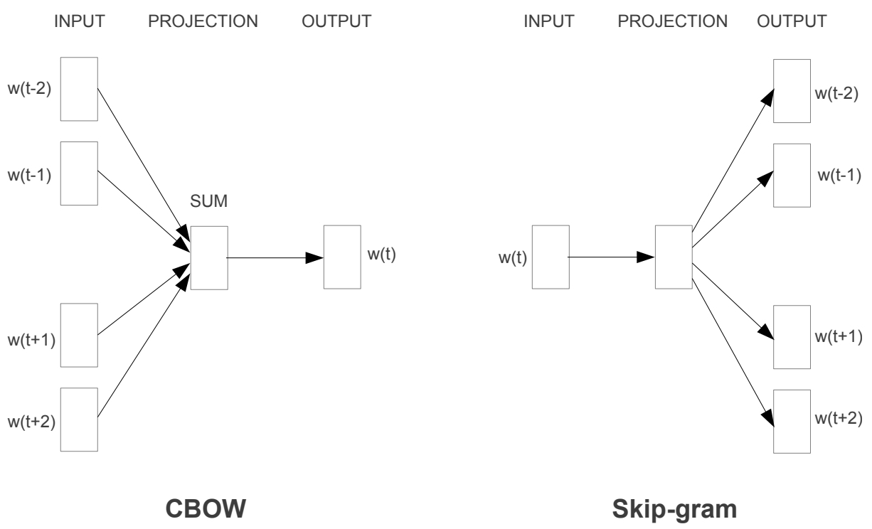
- Continuous Bag-of-Words (CBOW):
- This model predicts a target word based on its context words. CBOW computes the conditional probability of a target word given the context words surrounding it across a window of size k. The input is a summation of the word vectors of the surrounding context words, with the output being the current word.
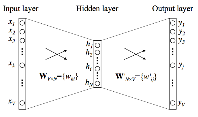
- Referring to the figure above (source), the CBOW model is a simple fully connected neural network with one hidden layer. The input layer, which takes the one-hot vector of context words, has \(\mathbf{V}\) neurons, while the hidden layer has \(\mathbf{N}\) neurons. The output layer is a softmax of all words in the vocabulary. The layers are connected by weight matrices \(\mathbf{W} \in \mathcal{R}^{V \times N}\) and \(\mathbf{W}^{\prime} \in \mathcal{R}^{N \times V}\). Each word from the vocabulary is finally represented as two learned vectors, \(\mathbf{v}_{\mathbf{c}}\) and \(\mathbf{v}_{\mathbf{w}}\), corresponding to context and target word representations, respectively. Thus, the \(k^{\text{th}}\) word in the vocabulary will have:
- Overall, for any word \(w_i\) with a given context word \(c\) as input:
- The parameters \(\theta=\left\{\mathbf{V}_{\mathbf{w}}, \mathbf{V}_{\mathbf{c}}\right\}\) are learned by defining the objective function as the log-likelihood and finding its gradient as:
- In the general CBOW model, all the one-hot vectors of context words are taken as input simultaneously, i.e.,
- This model predicts a target word based on its context words. CBOW computes the conditional probability of a target word given the context words surrounding it across a window of size k. The input is a summation of the word vectors of the surrounding context words, with the output being the current word.
- Continuous Skip-gram: Conversely, the Skip-gram model predicts the surrounding context words from a given target word. The input is the target word, and the output is a softmax classification over the entire vocabulary to predict the context words. Skip-gram does the exact opposite of the CBOW model by predicting the surrounding context words given the central target word. The context words are assumed to be located symmetrically to the target word within a distance equal to the window size in both directions.
- Continuous Bag-of-Words (CBOW):
-
The following figure from the paper shows the two Word2Vec model architectures. The CBOW architecture predicts the current word based on the context, and the skip-gram predicts surrounding words given the current word.
Training and Optimization
- The training of Word2Vec involves representing every word in a fixed vocabulary by a vector and then optimizing these vectors to predict surrounding words accurately. This is achieved through stochastic gradient descent, minimizing a loss function that indicates the discrepancy between predicted and actual context words. The algorithm uses a sliding window approach to maximize the probability of context words given a center word, as illustrated in the accompanying diagram:
Embedding and Semantic Relationships
- Through the training process, Word2Vec places words with similar meanings in proximity within the high-dimensional vector space. For example, ‘bread’ and ‘croissant’ would have closely aligned vectors, just as ‘woman’, ‘king’, and ‘man’ would demonstrate meaningful relationships through vector arithmetic:
Distinction from Traditional Models
- A key differentiation between Word2Vec and traditional count-based language models is its reliance on embeddings. Deep learning-based NLP models, including Word2Vec, represent words, phrases, and even sentences using these embeddings, which encode much richer contextual and semantic information.
Semantic Nature of Word2Vec Embeddings
- Word2Vec embeddings are considered semantic in the sense that they capture semantic relationships between words based on their usage in the text. The key idea behind Word2Vec is that words used in similar contexts tend to have similar meanings. This is often summarized by the phrase “a word is characterized by the company it keeps.”
- When Word2Vec is trained on a large corpus of text, it learns vector representations (embeddings) for words such that words with similar meanings have similar embeddings. This is achieved through either of two model architectures: Continuous Bag-of-Words (CBOW) or Skip-Gram.
- CBOW Model: This model predicts a target word based on context words. For example, in the sentence “The cat sat on the ___”, the model tries to predict the word ‘mat’ based on the context provided by the other words.
- Skip-Gram Model: This model works the other way around, where it uses a target word to predict context words. For instance, given the word ‘cat’, it tries to predict ‘the’, ‘sat’, ‘on’, and ‘mat’.
- These embeddings capture various semantic relationships, such as:
- Similarity: Words with similar meanings have embeddings that are close in the vector space.
- Analogy: Relationships like “man is to woman as king is to queen” can often be captured through vector arithmetic (e.g.,
vector('king') - vector('man') + vector('woman')is close tovector('queen')). - Clustering: Words with similar meanings tend to cluster together in the vector space.
- However, it’s important to note that while Word2Vec captures many semantic relationships, it also has limitations. For example, it doesn’t capture polysemy well (the same word having different meanings in different contexts) and sometimes the relationships it learns are more syntactic than semantic. More advanced models like BERT and GPT have since been developed to address some of these limitations.
Key Limitations and Advances in Word2Vec and Word Embeddings
-
Word2Vec, a pivotal development in natural language processing, has significantly advanced our understanding of semantic relationships between words through vector embeddings. However, despite its breakthrough status, Word2Vec and traditional word embeddings are not without limitations, many of which have been addressed in subsequent developments within the field.
- Static, Non-Contextualized Nature:
- Single Vector Per Word: Word2Vec assigns a unique vector to each word, which remains static regardless of the word’s varying context in different sentences. This results in a representation that cannot dynamically adapt to different usages of the same word.
- Combination of Contexts: In cases where a word like “bank” appears in multiple contexts (“river bank” vs. “financial bank”), Word2Vec does not generate distinct embeddings for each scenario. Instead, it creates a singular, averaged representation that amalgamates all the contexts in which the word appears, leading to a generalized semantic representation.
- Lack of Disambiguation: The model’s inability to differentiate between the multiple meanings of polysemous words means that words like “bank” are represented by a single vector, irrespective of the specific meaning in a given context.
- Context Window Limitation: Word2Vec employs a fixed-size context window, capturing only local co-occurrence patterns without a deeper understanding of the word’s role in the broader sentence or paragraph.
- Training Process and Computational Intensity:
- Adjustments During Training: Throughout the training process, the word vectors are continually adjusted, not to switch between meanings but to refine the word’s placement in the semantic space based on an aggregate of its various uses.
- Resource Demands: Training Word2Vec, particularly for large vocabularies, requires significant computational resources and time. Techniques like negative sampling were introduced to alleviate some of these demands, but computational intensity remains a challenge.
- Handling of Special Cases:
- Phrase Representation: Word2Vec struggles with representing phrases or idioms where the meaning is not simply an aggregation of the meanings of individual words. For instance, idioms like “hot potato” or named entities such as “Boston Globe” cannot be accurately represented by the combination of individual word embeddings. One solution, as explored by Mikolov et al. (2013), is to identify such phrases based on word co-occurrence and train embeddings for them separately. More recent methods have explored directly learning n-gram embeddings from unlabeled data.
- Out-of-Vocabulary Words: The model faces challenges with unknown or out-of-vocabulary (OOV) words. This issue is better addressed in models that treat words as compositions of characters, such as character embeddings, which are especially beneficial for languages with non-segmented scripts.
- Global Vector Representation Limitations:
- Uniform Representation Across Contexts: Word2Vec, like other traditional methods, generates a global vector representation for each word, which does not account for the various meanings a word can have in different contexts. For example, the different senses of “bank” in diverse sentences are not captured distinctively. This results in embeddings that are less effective in tasks requiring precise contextual understanding, such as sentiment analysis.
- Sentiment Polarity Issues: Learning embeddings based only on a small window of surrounding words can lead to words with opposing sentiment polarities (e.g., “good” and “bad”) sharing almost the same embedding. This is problematic in tasks such as sentiment analysis, where it is crucial to distinguish between these sentiments. Tang et al. (2014) addressed this issue by proposing sentiment-specific word embeddings (SSWE), which incorporate the supervised sentiment polarity of text in their loss functions while learning the embeddings.
- Resulting Embedding Compromises:
- The resulting vector for words with distinct meanings is a compromise that reflects its diverse uses, leading to less precise representations for tasks requiring accurate contextual understanding.
- These limitations of Word2Vec and traditional word embeddings have spurred advancements in the field, leading to the development of more sophisticated language models like BERT and ELMo. These newer models address issues of context sensitivity, polysemy, computational efficiency, and handling of OOV words, marking a significant progression in natural language processing.
Further Learning Resources
- For those interested in a deeper exploration of Word2Vec, the following resources provide comprehensive insights into the foundational aspects of Word2Vec:
Global Vectors for Word Representation (GloVe)
Overview
- Proposed in GloVe: Global Vectors for Word Representation by Pennington et al. (2014), Global Vectors for Word Representation (GloVe) embeddings are a type of word representation used in NLP. They are designed to capture not just the local context of words but also their global co-occurrence statistics in a corpus, thus providing a rich and nuanced word representation.
- By blending these approaches, GloVe captures a fuller picture of word meaning and usage, making it a valuable tool for various NLP tasks, such as sentiment analysis, machine translation, and information retrieval.
- Here’s a detailed explanation along with an example:
How GloVe Works
-
Co-Occurrence Matrix: GloVe starts by constructing a large matrix that represents the co-occurrence statistics of words in a given corpus. This matrix has dimensions of
[vocabulary size] x [vocabulary size], where each entry \((i, j)\) in the matrix represents how often word i occurs in the context of word j. -
Matrix Factorization: The algorithm then applies matrix factorization techniques to this co-occurrence matrix. The goal is to reduce the dimensions of each word into a lower-dimensional space (the embedding space), while preserving the co-occurrence information.
-
Word Vectors: The end result is that each word in the corpus is represented by a vector in this embedding space. Words with similar meanings or that often appear in similar contexts will have similar vectors.
-
Relationships and Analogies: These vectors capture complex patterns and relationships between words. For example, they can capture analogies like “man is to king as woman is to queen” by showing that the vector ‘king’ - ‘man’ + ‘woman’ is close to ‘queen’.
Example
- Imagine a simple corpus with the following sentences:
- “The cat sat on the mat.”
- “The dog sat on the log.”
- From this corpus, a co-occurrence matrix is constructed. For instance, ‘cat’ and ‘mat’ will have a higher co-occurrence score because they appear close to each other in the sentences. Similarly, ‘dog’ and ‘log’ will be close in the embedding space.
- After applying GloVe, each word (like ‘cat’, ‘dog’, ‘mat’, ‘log’) will be represented as a vector. The vector representation captures the essence of each word, not just based on the context within its immediate sentence, but also based on how these words co-occur in the entire corpus.
- In a large and diverse corpus, GloVe can capture complex relationships. For example, it might learn that ‘cat’ and ‘dog’ are both pets, and this will be reflected in how their vectors are positioned relative to each other and to other words like ‘pet’, ‘animal’, etc.
Significance of GloVe
- GloVe is powerful because it combines the benefits of two major approaches in word representation:
- Local Context Window Methods (like Word2Vec): These methods look at the local context, but might miss the broader context of word usage across the entire corpus.
- Global Matrix Factorization Methods: These methods, like Latent Semantic Analysis (LSA), consider global word co-occurrence but might miss the nuances of local word usage.
Limitations of GloVe
- While GloVe has been widely used and offers several rich word representations, it may not be the optimal choice for every NLP application, especially those requiring context sensitivity, handling of rare words, or efficient handling of computational resources as detailed below.
Lack of Context-Sensitivity
- Issue: GloVe generates a single, static vector for each word, regardless of the specific context in which the word is used. This can be a significant limitation, especially for words with multiple meanings (polysemy).
- Example: The word “bank” will have the same vector representation whether it refers to the side of a river or a financial institution, potentially leading to confusion in downstream tasks where context matters.
- Comparison: Modern models like BERT and GPT address this limitation by creating context-sensitive embeddings, where the meaning of a word can change based on the sentence or context in which it appears.
Inefficient for Rare Words
- Issue: GloVe relies on word co-occurrence statistics from large corpora, which means it may not generate meaningful vectors for rare words or words that don’t appear frequently enough in the training data.
- Example: Words that occur infrequently in a corpus will have less reliable vector representations, potentially leading to poor performance on tasks that involve rare or domain-specific vocabulary.
- Comparison: Subword-based models like FastText handle this limitation more effectively by creating word representations based on character n-grams, allowing even rare words to have meaningful embeddings.
Corpus Dependence
- Issue: The quality of the GloVe embeddings is highly dependent on the quality and size of the training corpus. If the corpus lacks diversity or is biased, the resulting word vectors will reflect these limitations.
- Example: A GloVe model trained on a narrow or biased dataset may fail to capture the full range of meanings or relationships between words, especially in domains or languages not well-represented in the corpus.
- Comparison: This issue is less pronounced in models like transformer-based architectures, where transfer learning allows fine-tuning on specific tasks or domains, reducing the dependence on a single corpus.
Computational Cost
- Issue: Training GloVe embeddings on large corpora involves computing and factorizing large co-occurrence matrices, which can be computationally expensive and memory-intensive.
- Example: The memory requirement for storing the full co-occurrence matrix grows quadratically with the size of the vocabulary, which can be prohibitive for very large datasets.
- Comparison: While Word2Vec also has computational challenges, GloVe’s matrix factorization step tends to be more resource-intensive than the shallow neural networks used by Word2Vec.
Limited to Word-Level Representation
- Issue: GloVe embeddings operate at the word level and do not directly handle subword information such as prefixes, suffixes, or character-level nuances.
- Example: Morphologically rich languages, where words can take many forms based on tense, gender, or plurality, may not be well-represented in GloVe embeddings.
- Comparison: FastText, in contrast, incorporates subword information into its word vectors, allowing it to better represent words in languages with complex morphology or in cases where a word is rare but its root form is common.
Inability to Handle OOV (Out-of-Vocabulary) Words
- Issue: Since GloVe produces fixed embeddings for words during the training phase, it cannot generate embeddings for words that were not present in the training corpus, known as Out-of-Vocabulary (OOV) words.
- Example: If a new or domain-specific word is encountered during testing or inference, GloVe cannot generate a meaningful vector for it.
- Comparison: Subword-based models like FastText or context-based models like BERT can mitigate this problem by creating embeddings dynamically, even for unseen words.
fastText
Overview
- Proposed in Enriching Word Vectors with Subword Information by Bojanowski et al. (2017), fastText is an advanced word representation and sentence classification library developed by Facebook AI Research (FAIR). It’s primarily used for text classification and word embeddings in NLP. fastText differs from traditional word embedding techniques through its unique approach to representing words, which is particularly beneficial for understanding morphologically complex languages or handling rare words.
- Specifically, fastText’s innovative approach of using subword information makes it a powerful tool for a variety of NLP tasks, especially in dealing with languages that have extensive word forms and in situations where the dataset contains many rare words. By learning embeddings that incorporate subword information, fastText provides a more nuanced and comprehensive understanding of language semantics compared to traditional word embedding methods.
- Here’s a detailed look at fastText with an example.
Core Features of fastText
-
Subword Information: Unlike traditional models that treat words as the smallest unit for training, fastText breaks down words into smaller units - subwords or character n-grams. For instance, for the word “fast”, with a chosen n-gram range of 3 to 6, some of the subwords would be “fas”, “fast”, “ast”, etc. This technique helps in capturing the morphology of words.
-
Handling of Rare Words: Due to its subword approach, fastText can effectively handle rare words or even words not seen during training. It generates embeddings for these words based on their subword units, allowing it to infer some meaning from these subcomponents.
-
Efficiency in Learning Word Representations: fastText is efficient in learning representations for words that appear infrequently in the corpus, which is a significant limitation in many other word embedding techniques.
-
Applicability to Various Languages: Its subword feature makes it particularly suitable for languages with rich word formations and complex morphology, like Turkish or Finnish.
-
Word Embedding and Text Classification: fastText can be used both for generating word embeddings and for text classification purposes, providing versatile applications in NLP tasks.
Example
- Consider the task of building a sentiment analysis model using word embeddings for an input sentence like “The movie was breathtakingly beautiful”. In traditional models like Word2Vec, each word is treated as a distinct unit, and if words like “breathtakingly” are rare in the training dataset, the model may not have a meaningful representation for them.
- With fastText, “breathtakingly” is broken down into subwords (e.g., “breat”, “eathtaking”, “htakingly”, etc.). fastText then learns vectors for these subwords. When computing the vector for “breathtakingly”, it aggregates the vectors of its subwords. This approach allows fastText to handle rare words more effectively, as it can utilize the information from common subwords to understand less common or even out-of-vocabulary words.
Limitations of fastText
- Despite its many strengths, fastText has several limitations that users should be aware of. These limitations can influence the effectiveness and appropriateness of fastText for certain NLP tasks, and understanding them can help users make more informed decisions when choosing word embedding models.
Limited Contextual Awareness
fastText operates on the principle of learning word embeddings by breaking down words into subwords. However, it does not consider the broader context in which a word appears within a sentence. This is because fastText, like Word2Vec, generates static embeddings, meaning that each word or subword is represented by the same vector regardless of its surrounding context.
For instance, the word “bank” in the sentences “He went to the bank to withdraw money” and “He sat by the river bank” will have the same embedding, even though the meanings are different in each case. More advanced models like BERT or GPT address this limitation by generating dynamic, context-sensitive embeddings.
Sensitivity to Subword Granularity
While fastText’s subword approach is one of its key strengths, it can also be a limitation depending on the language and task. The choice of n-grams (i.e., the length of subwords) can have a significant impact on the quality of embeddings. Selecting the wrong subword granularity may lead to suboptimal performance, as shorter n-grams might capture too much noise, while longer n-grams may fail to generalize effectively.
Furthermore, fastText might overemphasize certain subwords, leading to biases in word embeddings. For example, frequent subword combinations (e.g., prefixes and suffixes) might dominate the representation, overshadowing the contributions of other meaningful subword units.
Inability to Model Long-Distance Dependencies
fastText’s reliance on local subword features means it struggles to capture long-distance dependencies between words in a sentence. For instance, in sentences where key information is spread out over several words (e.g., “The man, who was wearing a red jacket, crossed the street”), fastText cannot effectively model relationships between the subject and the predicate when they are far apart. Models like LSTMs or transformers are more suited for handling such dependencies.
Scalability and Resource Requirements
While fastText is designed to be efficient, it still requires significant computational resources, especially when dealing with large corpora or many languages. Training models with large n-grams can increase both the memory and time required for training. In addition, the storage requirements for embeddings can grow substantially, particularly when generating embeddings for extensive vocabularies with numerous subwords.
Lack of Language-Specific Optimizations
Although fastText is well-suited for morphologically rich languages, it lacks the language-specific optimizations that some newer NLP models (like multilingual BERT) offer. fastText treats all languages uniformly, which can be a limitation for languages with unique syntactic or semantic characteristics that require specialized treatment. For example, languages with complex agreement systems or non-concatenative morphology might benefit from more tailored approaches than fastText provides.
Limited Performance in Highly Context-Dependent Tasks
fastText performs well in tasks where morphology and subword information play a key role, such as text classification or simple sentiment analysis. However, for highly context-dependent tasks such as machine translation, nuanced sentiment detection, or question-answering systems, fastText may not provide enough context sensitivity. More sophisticated models like transformers, which are designed to capture nuanced semantic and syntactic relationships, generally perform better in such scenarios.
BERT Embeddings
- For more details about BERT embeddings, please refer the BERT primer.
Handling Polysemous Words – Key Limitation of BoW, TF-IDF, BM25, Word2Vec, GloVe, and fastText
- BoW, TF-IDF, BM25, Word2Vec, GloVe, and fastText each have distinct ways of representing words and their meanings. However, all of these methods generate a single embedding per word, leading to a blended representation of different senses for polysemous words. This approach averages the contexts, which can dilute the specific meanings of polysemous words. Put simply, a major challenge across several of these methods is their inability to handle polysemous words (words with multiple meanings) effectively, often resulting in a single representation that blends different senses of the word. While later methods such as fastText provide some improvements by leveraging subword information, none fully resolves the issue of distinguishing between different senses of a word based on its context.
- BERT, on the other hand, overcomes this limitation by generating contextualized embeddings that adapt to the specific meaning of a word based on its surrounding context. This allows BERT to differentiate between multiple senses of a polysemous word, providing a more accurate representation.
- Below is a detailed examination of how each method deals with polysemy.
Bag of Words (BoW)
- Description:
- BoW is a simple method that represents text as a collection of words without considering grammar or word order. It counts the frequency of each word in a document.
- Handling Polysemy:
- Word Frequency:
- BoW does not create embeddings; instead, it treats each word as an individual token. Therefore, it cannot distinguish between different meanings of a word in different contexts.
- Context Insensitivity:
- The method cannot differentiate between polysemous meanings, as each occurrence of a word contributes equally to its frequency count, regardless of its meaning in context.
- Limitations:
- Since BoW lacks context sensitivity, polysemous words are treated as if they have only one meaning, which limits its effectiveness in capturing semantic nuances.
- Word Frequency:
TF-IDF (Term Frequency-Inverse Document Frequency)
- Description:
- TF-IDF refines BoW by considering how important a word is in a document relative to the entire corpus. It assigns higher weights to words that appear frequently in a document but less often in the corpus.
- Handling Polysemy:
- Term Weighting:
- TF-IDF improves over BoW by emphasizing less common but important words. However, it still treats each word as a unique token without considering its multiple meanings in different contexts.
- Context-Agnostic:
- Like BoW, TF-IDF does not distinguish between the different senses of polysemous words, as it focuses on term frequency without leveraging context.
- Limitations:
- While TF-IDF addresses term relevance, it remains unable to handle polysemous words accurately due to its single-representation approach.
- Term Weighting:
BM25
- Description:
- BM25 is an extension of TF-IDF, often used in information retrieval, which ranks documents based on the frequency of query terms but also considers document length and term saturation.
- Handling Polysemy:
- Rank-based Approach:
- BM25 assigns relevance scores to documents based on keyword matches, but like BoW and TF-IDF, it does not account for polysemy since it treats each occurrence of a word the same way.
- Context-Agnostic:
- While BM25 improves retrieval effectiveness through sophisticated term weighting, it still represents polysemous words as a single entity.
- Limitations:
- BM25 struggles with polysemy as it relies on exact word matches rather than distinguishing between different meanings of a word in different contexts.
- Rank-based Approach:
Word2Vec
- Description:
- Word2Vec includes two model architectures: Continuous Bag of Words (CBOW) and Skip-gram. Both learn word embeddings by predicting target words from context words (CBOW) or context words from a target word (Skip-gram).
- Handling Polysemy:
- Single Vector Representation:
- Word2Vec generates a single embedding for each word in the vocabulary, regardless of its context. This means that all senses of a polysemous word are represented by the same vector.
- Context Averaging:
- The embedding of a polysemous word is an average representation of all the contexts in which the word appears. For example, the word “bank” will have a single vector that averages contexts from both financial institutions and river banks.
- Limitations:
- This single-vector approach fails to capture distinct meanings accurately, leading to less precise embeddings for polysemous words.
- Single Vector Representation:
GloVe
- Description:
- GloVe is a count-based model that constructs word embeddings using global word-word co-occurrence statistics from a corpus. It learns embeddings by factorizing the co-occurrence matrix.
- Handling Polysemy:
- Single Vector Representation:
- Like Word2Vec, GloVe assigns a single embedding to each word in the vocabulary.
- Global Context:
- The embedding captures the word’s overall statistical context within the corpus. Thus, the different senses of polysemous words are combined into one vector.
- Limitations:
- Similar to Word2Vec, this blending of senses can dilute the quality of embeddings for polysemous words.
- Single Vector Representation:
fastText
- Description:
- fastText, developed by Facebook, extends Word2Vec by incorporating subword information. It represents words as bags of character n-grams, which allows it to generate embeddings for words based on their subword units.
- Handling Polysemy:
- Single Vector Representation:
- Although fastText incorporates subword information and can better handle rare words and morphologically rich languages, it still produces a single vector for each word.
- Subword Information:
- The inclusion of character n-grams can capture some nuances of polysemy, especially when different meanings have distinct morphological patterns. However, this is not a complete solution for polysemy.
- Limitations:
- While slightly better at representing polysemous words than Word2Vec and GloVe due to subword information, fastText still merges multiple senses into a single embedding.
- Single Vector Representation:
BERT
- Description:
- BERT is a transformer-based model that generates contextual embeddings by considering both the left and right context of a word in a sentence. Unlike Word2Vec and GloVe, BERT produces different embeddings for the same word depending on the surrounding context.
- Handling Polysemy:
- Contextualized Embeddings:
- BERT addresses the limitations of previous models by creating unique embeddings for polysemous words based on their specific usage within a sentence. For example, the word “bank” in the sentence “I went to the river bank” will have a different embedding than “I deposited money at the bank.”
- Dynamic Representation:
- BERT captures the different meanings of polysemous words by analyzing the entire sentence, thereby generating representations that are highly sensitive to context.
- Advancements Over Single-Vectors:
- Unlike Word2Vec, GloVe, or fastText, BERT is not constrained to a single-vector representation for polysemous words. It dynamically adapts to the specific sense of a word in each context, offering a significant improvement in handling polysemy.
- Limitations:
- Although BERT excels in handling polysemy, its computational complexity is higher, requiring more resources for both training and inference. Additionally, it requires large amounts of data to fine-tune effectively for domain-specific applications.
- Contextualized Embeddings:
Example: BoW, TF-IDF, BM25, Word2Vec, GloVe, fastText, and BERT Embeddings
- Let’s expand on the example involving the word “cat” to illustrate how different embedding techniques (BoW, TF-IDF, BM25, Word2Vec, GloVe, fastText, and BERT) might represent it. We’ll consider the same documents as before:
- Document 1: “Cat sat on the mat.”
- Document 2: “Dog sat on the log.”
- Document 3: “Cat chased the dog.”
Bag of Words (BoW) Representation for “Cat”
- Bag of Words is one of the simplest forms of word representation. In this method, each document is represented as a vector of word counts. The position of each word in the vector corresponds to the presence or absence (or count) of the word in the document, regardless of the word order.
- For example, consider a vocabulary consisting of the words {cat, sat, on, the, mat, dog, log, chased}. The BoW vectors for each document would be:
- Document 1:
[1, 1, 1, 1, 1, 0, 0, 0](because the words “cat”, “sat”, “on”, “the”, and “mat” each appear once). - Document 2:
[0, 1, 1, 1, 0, 1, 1, 0](because “dog”, “sat”, “on”, “the”, and “log” appear). - Document 3:
[1, 0, 0, 1, 0, 1, 0, 1](because “cat”, “the”, “dog”, and “chased” appear).
- Document 1:
- BoW Representation for “Cat”:
[1, 0, 1](the word “cat” appears once in Document 1 and once in Document 3, but not in Document 2).
TF-IDF Embedding for “Cat”
- In TF-IDF, each word in a document is assigned a weight. This weight increases with the number of times the word appears in the document but is offset by the frequency of the word in the corpus.
- TF-IDF assigns a weight to a word in each document, reflecting its importance. The steps are:
- Calculate Term Frequency (TF): Count of “cat” in each document divided by the total number of words in that document.
- Calculate Inverse Document Frequency (IDF): Logarithm of the total number of documents divided by the number of documents containing “cat”.
- Multiply TF by IDF for each document.
- For instance, the TF-IDF weight for the word “cat” in Document 1 would be calculated as follows (simplified calculation):
- Term Frequency (TF) of “cat” in Document 1 = 1/5 (it appears once out of five words).
- Inverse Document Frequency (IDF) of “cat” = log(3/2) (it appears in 2 out of 3 documents, and we use the logarithm to dampen the effect).
- TF-IDF for “cat” in Document 1 = TF * IDF = (1/5) * log(3/2).
- Final TF-IDF Embedding for “Cat”:
[0.18, 0, 0.18](assuming normalized values for simplicity).
BM25 Embedding for “Cat”
- BM25 builds on top of TF-IDF and thus is more complex than TF-IDF. It considers term frequency, document frequency, document length, and two parameters: k1 and b. The final BM25 score for “cat” in each document might look like this (assuming certain values for \(k1\) and \(b\)):
- Final BM25 Score for “Cat”:
[2.5, 0, 2.3](hypothetical values).
Word2Vec Embedding for “Cat”
- Word2Vec provides a dense vector for each word. This vector is learned based on the context in which the word appears across the entire corpus, not just our three documents as in the example above.
- The model might represent the word “cat” as a vector, such as
[0.76, -0.21, 0.58, ...](assuming a 3-dimensional space for simplicity, but in reality, these vectors often have hundreds of dimensions).
GloVe Embedding for “Cat”
- GloVe, like Word2Vec, provides a dense vector for each word based on the aggregate global word-word co-occurrence statistics from a corpus.
- Hypothetical GloVe Embedding for “Cat”: In a 3-dimensional space,
[0.81, -0.45, 0.30]. As with Word2Vec, real-world GloVe embeddings would have a much higher dimensionality.
In these examples, it’s important to note that the BoW, TF-IDF, and BM25 scores depend on the context of the specific documents, whereas the Word2Vec and GloVe embeddings are more general, trained on a larger corpus and representing the word’s meaning in a broader context. On the flip side, Word2Vec, GloVe, and fastText embeddings, lack contextualized representations (so they cannot represent polysemous works effectively), however, models such as ELMo and BERT overcome that limitation using contextualized embeddings. The specific values used here for TF-IDF, BM25, Word2Vec, and GloVe are illustrative and would vary based on the actual computation and dimensions used.
fastText Embedding for “Cat”
- fastText, like Word2Vec and GloVe, is a method for learning word embeddings, but it differs in its treatment of words. fastText treats each word as a bag of character n-grams, which allows it to better represent rare words or words not seen during training by breaking them down into smaller units.
- Hypothetical fastText Embedding for “Cat”: Assuming a 3-dimensional space,
[0.72, -0.25, 0.63]. Like the others, real fastText embeddings typically have a much higher dimensionality. - In this expanded example, the key addition of fastText is its ability to handle out-of-vocabulary words by breaking them down into n-grams, offering a more flexible representation, especially for languages with rich morphology or a lot of word forms. The specific values for fastText, like the others, are illustrative and depend on the actual corpus and training setup.
BERT Embedding for “Cat”
-
BERT (Bidirectional Encoder Representations from Transformers) is a transformer-based model that generates contextualized word embeddings, meaning the representation of a word depends on the surrounding words in the sentence. Unlike static embeddings (Word2Vec, GloVe, fastText), BERT captures the various meanings (polysemy) of a word based on its context. This makes BERT powerful for handling ambiguous or polysemous words like “cat,” whose meaning might change depending on how it’s used in a sentence.
- For example, BERT would generate different embeddings for “cat” in the following contexts:
- Document 1: “Cat sat on the mat.”
- Document 3: “Cat chased the dog.”
-
Here, the word “cat” in Document 1 might be represented as a vector like
[0.65, -0.34, 0.77, ...], indicating a relaxed or neutral context, while in Document 3, where “cat” is involved in an action (“chased”), it might generate a different embedding like[0.78, -0.10, 0.89, ...]. -
Unlike traditional word embeddings, BERT’s ability to incorporate both the left and right context enables a nuanced understanding of each occurrence of “cat.” These vectors would be different not only based on the sentence but also based on the larger document context in which the word appears.
- BERT Embedding for “Cat”: Instead of a static embedding like
[0.76, -0.21, 0.58](as in Word2Vec or GloVe), BERT might output[0.65, -0.34, 0.77]in one sentence and a different vector[0.78, -0.10, 0.89]for “cat” in another, demonstrating its strength in understanding word meaning based on context.
BERT embeddings are useful in tasks like question answering, text classification, and named entity recognition, where understanding the specific meaning of a word in its context is critical. By leveraging bidirectional attention, BERT improves significantly over previous models that treat words in isolation or with limited context.
Summary: Types of Embeddings
- In the field of NLP, a variety of embedding techniques have been developed, each suited to specific applications and use cases. This article categorizes and delves into different types of word embeddings and their functionalities.
Bag-of-Words-based Embeddings
- These embeddings do not consider the order of words.
- Bag of Words (BoW): The simplest text representation method, BoW is a count-based approach that tallies the occurrences of each word in a document. However, it disregards any information about the order or structure of words, treating the text as a mere “bag” of words. It focuses only on the presence or absence of words, not their positioning within the document.
- TF-IDF (Term Frequency-Inverse Document Frequency): An advanced version of count vectors, TF-IDF considers the frequency of words in a document as well as their overall frequency in the corpus. Common words like “the” have lower TF-IDF scores, while unique or rare words have higher scores, reflecting their relative importance.
Predictive Word Embeddings
- These models predict words based on their context.
- Word2Vec: A neural network-based model that learns to represent words as vectors in a high-dimensional space. Words with similar meanings are represented by proximate vectors. Word2Vec facilitates capturing meanings, semantic similarities, and relationships within text, exemplified by analogies like
king - man + woman = queen.
- Word2Vec: A neural network-based model that learns to represent words as vectors in a high-dimensional space. Words with similar meanings are represented by proximate vectors. Word2Vec facilitates capturing meanings, semantic similarities, and relationships within text, exemplified by analogies like
Contextual and Sequential Data Embeddings
- Representing order and context of words, and suited for sequential data like text.
- Recurrent Neural Networks (RNNs): RNNs, and their advanced variants like LSTMs (Long Short-Term Memory), are adept at handling sequential data. They process inputs in a sequence, with each step’s output feeding into the next, capturing information from previous steps.
- Transformer: A model that revolutionized NLP with its encoder-decoder architecture, leveraging self-attention mechanisms. Transformers excel in learning long-range dependencies, allowing them to focus on specific parts of the input sequence and better understand sentence meanings.
Contextual Embeddings
-
These consider the order and context of words.
- ELMo (Embeddings from Language Models): Generates contextual embeddings from the internal states of a bi-directional LSTM.
- BERT (Bidirectional Encoder Representations from Transformers) Embeddings: Provides contextual embeddings based on the entire context of word usage.
Sentence/Document Embeddings
-
For broader textual units like sentences or documents.
- Doc2Vec: Extends Word2Vec to represent entire documents.
- Sentence-BERT: Adapts BERT for sentence-level embeddings.
- Universal Sentence Encoder: Encodes sentences into vectors for various tasks.
Positional Embeddings
-
Encodes the position of words within sequences.
- Absolute Positional Embeddings: Used in Transformers to encode the absolute position of words.
- Relative Positional Embeddings: Focuses on relative distances between words, beneficial in models like Transformer-XL and T5.
- Rotary Positional Embeddings/RoPE (Rotary Positional Encoding): Employs rotational operations to encode relative positions.
Relative Embeddings
-
Capture relative positions between word pairs in sequences.
- Relative Positional Embeddings: Encodes the relative positioning of words, like in the sentence “Alice threw the ball to Bob,” where “ball” has a relative position to other words. In Transformer models, the difference between positions \(i\) and \(j\) in the input sequence is used to retrieve corresponding embedding vectors, enhancing the model’s ability to generalize to new sequence lengths.
-
This categorization of embedding techniques underscores the diversity and evolution of approaches in representing linguistic elements in NLP, each with distinct advantages and suited for specific applications.
Comparative Analysis of BoW, TF-IDF, BM25, Word2Vec, GloVe, fastText, and BERT Embeddings
- Each of these techniques represents a different approach to encoding text data for tasks like search, document classification, sentiment analysis, and more. Each method has its strengths and weaknesses, making them suitable for different tasks based on the trade-offs of simplicity vs. semantic richness and computational efficiency. Let’s break them down one by one, comparing their approaches, advantages, disadvantages, and use cases.
Bag of Words (BoW)
- Description:
- BoW is the simplest form of text representation where a document is represented as a vector of word counts, without any regard to word order or meaning.
- It creates a vocabulary of unique words from the corpus and then encodes each document based on the frequency of these words.
- How it works:
- Create a vocabulary of all unique words.
- For each document, count the occurrence of each word in the vocabulary and represent the document as a vector of these counts.
- Advantages:
- Simple and easy to implement.
- Works well when word order and semantics are not important.
- Disadvantages:
- Ignores semantics and word order (no understanding of the meaning or relationships between words).
- High dimensionality (especially with large vocabularies).
- Sparsity of vectors (most values are zero since many words will not appear in every document).
- Use Cases:
- Text classification, simple document similarity tasks, and basic Natural Language Processing (NLP) problems.
Term Frequency-Inverse Document Frequency (TF-IDF)
- Description:
- TF-IDF improves upon BoW by weighting words based on their frequency in a document (Term Frequency, TF) and the rarity of the word across the corpus (Inverse Document Frequency, IDF). Words that are common in many documents receive lower weights.
- How it works:
- TF is the frequency of a term in a document.
- IDF is calculated as the logarithm of the total number of documents divided by the number of documents that contain the term.
- The final TF-IDF score is the product of TF and IDF.
- Advantages:
- Reduces the importance of common words (like “the,” “and”) that provide little discriminative power.
- More informative than BoW by highlighting rare but significant words.
- Disadvantages:
- Still ignores the word order and contextual relationships.
- Suffers from sparsity and high dimensionality like BoW.
- Does not capture deep semantics or relationships between words.
- Use Cases:
- Information retrieval, text ranking, document classification, and keyword extraction.
BM25 (Best Matching 25)
- Description:
- BM25 is a ranking function used by search engines, building on the TF-IDF concept but incorporating additional factors like term saturation and document length normalization. It ranks documents based on how relevant they are to a given query.
- How it works:
- Similar to TF-IDF, but uses a non-linear saturation function for term frequency and adjusts based on document length. It considers term frequency more naturally, as the contribution of a term to the score increases but saturates after a certain point.
- Advantages:
- A more sophisticated version of TF-IDF that captures term importance more naturally.
- Handles variations in document length and term frequency saturation better than TF-IDF.
- Disadvantages:
- Still based on a bag-of-words model, so it does not capture word semantics or order.
- Limited to ranking tasks and cannot be directly used for other tasks like word embeddings.
- Use Cases:
- Search engines, information retrieval, query-document ranking.
Word2Vec
Description:
- Word2Vec is a neural network-based model that creates dense word embeddings. It maps words into a continuous vector space such that words with similar meanings are close to each other in the vector space.
-
It comes in two flavors: CBOW (Continuous Bag of Words) and Skip-gram.
- How it works:
- CBOW predicts a word given its surrounding context.
- Skip-gram predicts the surrounding context given a word.
- Both models learn vector representations for words based on co-occurrence patterns in large corpora.
- Advantages:
- Captures semantic relationships between words (e.g., “king” - “man” + “woman” ≈ “queen”).
- Dense vectors with much lower dimensionality compared to BoW or TF-IDF.
- Captures analogy relations (e.g., “Paris is to France as Berlin is to Germany”).
- Disadvantages:
- Context-independent: the same word always has the same vector regardless of its meaning in different contexts.
- Requires large amounts of data to train good embeddings.
- Use Cases:
- Semantic similarity, analogy reasoning, clustering, and as input for downstream NLP models.
GloVe (Global Vectors for Word Representation)
- Description:
- GloVe is also a word embedding model, but it is based on matrix factorization of the co-occurrence matrix of words in a corpus. It attempts to capture both local context and global word statistics.
- How it works:
- First, a word co-occurrence matrix is built, which records how often words appear together in a corpus.
- Then, this matrix is factorized to obtain word embeddings. The objective is to predict the ratio of probabilities of word co-occurrence.
- Advantages:
- Combines the benefits of co-occurrence statistics (global context) and local context-based methods like Word2Vec.
- Dense embeddings, capturing semantic relationships.
- Disadvantages:
- Like Word2Vec, it generates context-independent embeddings.
- Requires large corpora to learn good-quality embeddings.
- Use Cases:
- Similar to Word2Vec: used in semantic similarity tasks, text classification, and input embeddings for other NLP models.
fastText
- Description:
- fastText is an extension of the Word2Vec model, developed by Facebook AI Research, that incorporates subword information into word embeddings. This allows fastText to create better representations of rare words and handle words with typos or variations. It represents each word as a bag of character n-grams, allowing it to capture morphology and word structure.
- How it works:
- fastText breaks down words into character-level n-grams and learns vector representations for both the words and their n-grams. The final word vector is the sum of its constituent n-grams. This approach captures word morphology and helps in generating meaningful embeddings even for unseen words or rare words.
- Advantages:
- Handles rare words, typos, and out-of-vocabulary (OOV) words by leveraging subword information.
- Dense and low-dimensional embeddings, similar to Word2Vec, but with more robustness for morphologically rich languages.
- Faster to train and can generate embeddings on-the-fly for unseen words.
- Disadvantages:
- Like Word2Vec and GloVe, fastText produces context-independent embeddings, meaning the same word has the same vector regardless of the sentence it appears in.
- It still operates primarily at the word level, so while it captures subword information, it does not account for the full sentence context like BERT.
- Use Cases:
- Useful in tasks involving rare or morphologically complex words, such as text classification, named entity recognition, and search in languages with rich word forms or frequent misspellings. It is also used for tasks like language modeling, sentence classification, and similarity detection.
BERT (Bidirectional Encoder Representations from Transformers)
Description:
-
BERT is a transformer-based deep learning model that creates contextualized embeddings for words. It differs from Word2Vec and GloVe by considering the full context of a word (both left and right) rather than just local context.
- How it works:
- Uses a transformer architecture to learn embeddings from large-scale unsupervised text data (such as Wikipedia).
- BERT is pre-trained on two tasks: Masked Language Modeling (MLM) and Next Sentence Prediction (NSP).
- MLM trains BERT to predict missing words in a sentence, while NSP helps it understand sentence relationships.
- Advantages:
- Contextual embeddings: the representation of a word changes depending on the context in which it appears.
- Handles polysemy effectively (e.g., different meanings of the word “bank” are represented differently based on the sentence).
- Captures deep semantic and syntactic relationships.
- Disadvantages:
- Computationally expensive and requires significant resources for training and inference.
- Large model size, making it harder to deploy in resource-constrained environments.
- Use Cases:
- Question answering, text classification, named entity recognition, and other advanced NLP tasks.
Comparative Summary
Count-Based Techniques (TF-IDF and BM25)
Pros
- Simplicity and Efficiency: Easy to implement and computationally efficient, suitable for basic information retrieval tasks.
- Effectiveness in Document Retrieval: Particularly good at identifying documents relevant to specific terms, thanks to their focus on term frequency.
Cons
- Lack of Semantic Understanding: They don’t capture deeper semantic relationships between words, leading to limited contextual interpretation.
- Sparse Representations: Can result in high-dimensional and sparse vectors, which are less efficient for complex NLP tasks.
Co-occurrence Based/Static Embedding Techniques (Word2Vec, GloVe, fastText)
Pros
- Semantic Relationship Modeling: Capable of capturing complex semantic relationships between words, offering richer representations.
- Subword Information (fastText): fastText’s consideration of subword elements aids in understanding morphology and handling out-of-vocabulary words.
Cons
- Fixed Context: Static embeddings assign a single, context-independent representation to each word, limiting their effectiveness in contextually varied scenarios.
- Computational Intensity: Requires significant computational resources for training on large corpora.
Contextualized Representation Techniques (BERT, ELMo)
Pros
- Context-Sensitive: They provide dynamic word representations based on context, leading to a more nuanced understanding of language.
- State-of-the-Art Performance: Excel in a wide range of NLP tasks, offering superior performance compared to previous models.
Cons
- Computational Requirements: Demand extensive computational power and larger datasets for training.
- Complexity in Implementation: More complex to implement and integrate into applications compared to simpler models like TF-IDF.
| Method | Type | Captures Semantics? | Dimensionality | Contextual? | Computational Complexity | Pros | Cons |
|---|---|---|---|---|---|---|---|
| BoW | Frequency-based | No | High | No | Low | - Simple and easy to implement. - Fast for small datasets. |
- Ignores word order and semantics. - Very high-dimensional and sparse. |
| TF-IDF | Frequency-based | Limited | High | No | Low | - Reduces impact of common words. - Simple and interpretable. |
- Still high-dimensional and sparse. - No deep semantic understanding. |
| BM25 | Frequency-based | Limited | High | No | Moderate | - More effective ranking than TF-IDF. - Considers document length and term saturation. |
- Complex for non-ranking tasks. - Still a bag-of-words model with no semantics. |
| Word2Vec | Embedding-based | Yes (basic) | Low | No | Moderate | - Dense, low-dimensional vectors. - Captures basic semantic relationships. |
- Context-independent embeddings. - Requires large corpora for good results. |
| GloVe | Embedding-based | Yes (basic) | Low | No | Moderate | - Combines local and global context. - Dense vectors and efficient embeddings. |
- Context-independent like Word2Vec. - Requires pre-training on large datasets. |
| fastText | Embedding-based | Yes (basic) | Low | No | Moderate | - Captures subword information. - Works well with rare words or misspellings. |
- Context-independent embeddings. - Limited to word-level representations. |
| BERT | Embedding-based | Yes (rich) | Low | Yes | High | - Contextualized embeddings capture deep meaning. - Handles polysemy effectively. |
- Computationally expensive and slow. - Large model size, hard to deploy on scale. |
Key Takeaways
- BoW and TF-IDF are simple, interpretable, and fast but fail to capture meaning and relationships between words.
- BM25 refines TF-IDF for better ranking performance but shares similar limitations.
- Word2Vec and GloVe generate dense embeddings that capture semantic relationships but are context-independent.
- fastText builds on Word2Vec by incorporating subword information, making it more robust to rare words, misspellings, and morphologically rich languages, though it remains context-independent.
- BERT is a state-of-the-art model that generates contextualized embeddings, making it the most powerful for complex NLP tasks but at the cost of high computational resources.
FAQs
What does the “Continuous” in Word2Vec’s Continuous Bag of Words and Continuous Skipgram refer to?
- The term “continuous” in Word2Vec’s Continuous Bag of Words (CBOW) and Continuous Skipgram models refers to the continuous and distributed representation of words in the vector space. This is in contrast to traditional bag-of-words models, which represent words using discrete and sparse vectors.
Traditional Bag of Words
- Discrete Representation:
- In a traditional Bag of Words model, each word is represented as a unique index in a vocabulary, creating a sparse and high-dimensional vector. For example, in a vocabulary of 10,000 words, “cat” might be represented as a vector with a 1 in the position corresponding to “cat” and 0s elsewhere.
- Sparse Vectors:
- These vectors are sparse because most elements are zero. Each word vector is orthogonal to every other word vector, meaning there is no inherent similarity between words represented in this way.
- No Context:
- BoW models do not capture the context in which words appear. They only consider word frequencies within documents, ignoring word order and contextual relationships.
Continuous Bag of Words
- Continuous and Distributed Representation:
- The “continuous” in CBOW refers to the use of continuous and dense vectors to represent words. Instead of sparse vectors, each word is mapped to a dense vector of real numbers. These vectors are typically of much lower dimensionality (e.g., 100 or 300 dimensions) and are learned through training on a large corpus.
- Contextual Embeddings:
- CBOW captures the context of a word by considering its surrounding words. Given a context (the words surrounding a target word), CBOW predicts the target word. For example, in the sentence “The cat sat on the mat,” the context for “sat” might be
["The", "cat", "on", "the", "mat"].
- CBOW captures the context of a word by considering its surrounding words. Given a context (the words surrounding a target word), CBOW predicts the target word. For example, in the sentence “The cat sat on the mat,” the context for “sat” might be
- Training Process:
- The model learns to maximize the probability of the target word given its context. This is done using a neural network that adjusts the word vectors to make similar words (words that appear in similar contexts) have similar vector representations.
- Dense Vectors:
- Each word is associated with a dense vector that captures various syntactic and semantic properties. These vectors are “continuous” in that they can take on any value in the real-number space, unlike the discrete indices used in traditional BoW models.
- Example:
- Suppose “cat” is represented by a 100-dimensional vector like
[0.25, -0.1, 0.75, ...]. This vector is learned from the contexts in which “cat” appears, and words that appear in similar contexts (like “dog”) will have similar vectors.
- Suppose “cat” is represented by a 100-dimensional vector like
Continuous Skipgram
- Continuous and Distributed Representation:
- Similar to CBOW, the “continuous” in the Continuous Skipgram model refers to the continuous and dense word vectors used to represent words. These vectors are also of lower dimensionality and are learned from large corpora.
- Reverse Prediction:
- Unlike CBOW, which predicts the target word from its context, Skipgram does the reverse: it predicts the context words given a target word. For example, in the sentence “The cat sat on the mat,” Skipgram would take “sat” as the input and try to predict words like “cat,” “on,” “the,” and “mat.”
- Training Process:
- The Skipgram model learns to predict the surrounding words of a given target word by adjusting the word vectors during training. The objective is to maximize the probability of context words given the target word, ensuring that words appearing in similar contexts end up with similar vector representations.
- Dense Vectors:
- Like CBOW, Skipgram also uses dense vectors to represent words. These vectors are continuous and can capture intricate relationships between words based on their context in a corpus.
- Example:
- If “sat” is represented by a 100-dimensional vector
[0.12, -0.3, 0.58, ...], the Skipgram model would adjust this vector during training to maximize the likelihood of predicting context words like “cat” and “on” when “sat” is the input.
- If “sat” is represented by a 100-dimensional vector
Key Advantages of CBOW and Skipgram
- Captures Contextual Information:
- Both models capture contextual relationships between words, leading to more meaningful word representations. CBOW does this by predicting the target word from its context, while Skipgram predicts the context from the target word.
- Dense and Low-Dimensional Vectors:
- The use of dense, continuous vectors reduces the dimensionality of the word representation, making it computationally more efficient and enabling the model to generalize better.
- Semantic Similarity:
- Words with similar meanings or that appear in similar contexts will have similar embeddings, allowing for better semantic understanding.
- Efficient Training:
- CBOW is generally faster to train than Skipgram because it uses the entire context to predict the target word, while Skipgram can better capture rare word associations by focusing on predicting the context from the target word.
Summary
- The “continuous” in both CBOW and Skipgram highlights the transition from discrete, sparse word representations to continuous, dense vector representations. This shift allows these models to capture contextual information and semantic relationships between words more effectively, leading to more powerful and meaningful word embeddings. CBOW excels in efficiency, while Skipgram often provides richer representations for rare words due to its reverse prediction approach.
How are Word2Vec, GloVe, and fastText Co-occurrence-based Embedding Techniques?
- Word2Vec, GloVe, and FastText are all co-occurrence-based embedding techniques, but they differ in their approaches to leveraging co-occurrence information to learn word embeddings. Here’s a detailed explanation of each method and how they utilize co-occurrence information:
Word2Vec
- Description:
- Word2Vec, developed by Google, includes two model architectures: Continuous Bag of Words (CBOW) and Skip-gram.
- Co-occurrence Information:
- CBOW: Predicts a target word based on the context words (words surrounding the target word within a fixed window size). This approach implicitly leverages word co-occurrence within the context window to learn embeddings.
- Skip-gram: Predicts context words given a target word. This method also relies on co-occurrence information within a fixed window around the target word.
- Training Objective: Both CBOW and Skip-gram use neural networks to optimize the embeddings so that words appearing in similar contexts have similar vectors.
- The models learn embeddings by maximizing the probability of predicting context words given a target word (Skip-gram) or predicting a target word given context words (CBOW).
GloVe
- Description:
- GloVe, developed by researchers at Stanford, is explicitly designed to capture global statistical information from a corpus by factorizing the word-word co-occurrence matrix.
- Co-occurrence Information:
- Co-occurrence Matrix: GloVe constructs a large sparse matrix where each cell represents the co-occurrence frequency of a pair of words within a specific context window.
- Objective Function: GloVe’s training objective is to factorize this co-occurrence matrix to produce word vectors. It aims to ensure that the dot product of word vectors approximates the logarithm of the words’ co-occurrence probabilities.
- Global Context: Unlike Word2Vec, which focuses on local context within a sliding window, GloVe captures global co-occurrence statistics across the entire corpus.
FastText
- Description:
- FastText, developed by Facebook, extends Word2Vec by incorporating subword information, representing words as bags of character n-grams.
- Co-occurrence Information:
- Subword Level Co-occurrence: FastText builds on the Skip-gram model of Word2Vec but adds a layer of granularity by considering subwords (character n-grams). This means that it leverages co-occurrence information at both the word level and the subword level.
- Training Objective: Similar to Skip-gram, FastText predicts context words from a target word, but it enriches the embeddings with subword information, allowing it to better handle rare and morphologically rich words.
- Enhanced Co-occurrence Handling: By incorporating subword information, FastText captures more detailed co-occurrence patterns, especially beneficial for languages with rich morphology or for handling out-of-vocabulary words.
Summary of Co-occurrence Based Techniques
- Word2Vec: Uses local co-occurrence information within a context window around each word. It learns embeddings by optimizing the prediction of target-context word pairs through neural networks (CBOW and Skip-gram models).
- GloVe: Utilizes global co-occurrence statistics from the entire corpus by factorizing a co-occurrence matrix. It explicitly captures how frequently words co-occur across the corpus, aiming to directly model the co-occurrence probabilities.
-
FastText: Extends the Skip-gram model to include subword information, leveraging both word-level and subword-level co-occurrence information. This approach helps to capture more fine-grained co-occurrence patterns and improves handling of rare or complex words.
- Each of these methods leverages co-occurrence information to learn word embeddings, but they do so in different ways and with varying levels of granularity, ranging from local context windows (Word2Vec) to global co-occurrence matrices (GloVe) and subword-level details (FastText).
Does Word2Vec use word-level or sub-word-level tokenization?
- Word2Vec uses word-level tokenization, meaning that it treats each word as a distinct unit or token, while other models like FastText use subword tokenization to overcome some of the limitations of Word2Vec. The Word2Vec model is designed to create embeddings for individual words based on their co-occurrence with other words in a large corpus. It does not natively break words down into smaller units, such as subwords, prefixes, or suffixes.
Key Points
- Word-level tokenization: In Word2Vec, each word is treated as an atomic entity, and embeddings are learned for each unique word in the vocabulary. This means words like “run” and “running” would have separate embeddings, without any explicit shared representation of the “run” root.
- Vocabulary limitations: One drawback of word-level tokenization in Word2Vec is that it doesn’t handle out-of-vocabulary (OOV) words well. If a word is not in the training corpus, the model won’t have an embedding for it. Similarly, it cannot generalize across words with similar morphological structures.
Sub-word-level Tokenization
- Sub-word tokenization (breaking words into smaller units like character n-grams, morphemes, or subwords) is handled by models like FastText or Byte Pair Encoding (BPE) in models such as BERT. For example, FastText builds on Word2Vec by learning embeddings not just for words but for character n-grams, enabling it to generalize better to unseen words and handle morphological variations.
Related: Matryoshka Representation Learning
- Proposed in Matryoshka Representation Learning by Kusupati et al. from UW, Matryoshka Representation Learning (MRL) is a novel approach for adaptive and efficient representation learning. This technique, adopted in OpenAI’s latest embedding update, text-embedding-3-large, is characterized by its ability to encode information at multiple granularities within a single high-dimensional vector. Drawing an analogy from the Russian Matryoshka dolls, MRL encapsulates details at various levels within a single embedding structure, allowing for adaptability to the computational and statistical needs of different tasks.
- The essence of MRL lies in its ability to create coarse-to-fine representations, where earlier dimensions in the embedding vector store more crucial information, and subsequent dimensions add finer details. You can understand how this works by the analogy of trying to classify an image at multiple resolutions – the lower resolutions give high-level info and the higher resolutions add finer details – human perception of the natural world also has a naturally coarse-to-fine granularity, as shown in the animation below.

- MRL achieves this by modifying the loss function in the model, where the total loss is the sum of losses over individual vector dimension ranges: \(Loss_{Total} = L(\text{upto 8d}) + L(\text{upto 16d}) + L(\text{upto 32d}) + \ldots + L(\text{upto 2048d})\). As a result, MRL incentivizes the model to capture essential information in each subsection of the vector. Notably, this technique allows for the use of any subset of the embedding dimensions, offering flexibility beyond fixed dimension slices like 8, 16, 32, etc.
- The figure below from the paper shows that MRL is adaptable to any representation learning setup and begets a Matryoshka Representation \(z\) by optimizing the original loss \(L(.)\) at \(O(\log(d))\) chosen representation sizes. Matryoshka Representation can be utilized effectively for adaptive deployment across environments and downstream tasks.
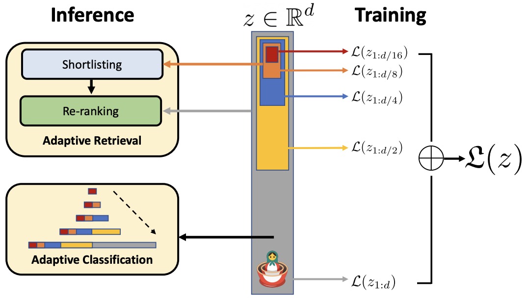
- MRL’s adaptability extends to a wide range of modalities, including vision, vision+language, and language models (such as ViT, ResNet, ALIGN, and BERT). The method has shown remarkable results in various applications, such as adaptive classification and retrieval, robustness evaluations, few-shot and long-tail learning, and analyses of model disagreement. In practical terms, MRL facilitates up to 14x smaller embedding sizes for tasks like ImageNet-1K classification without compromising accuracy, up to 14x real-world speed-ups for large-scale retrieval, and up to 2% accuracy improvements in long-tail few-shot classification.
- One of the striking outcomes of using MRL is demonstrated in OpenAI’s text-embedding-3-large model, which, when trimmed to 256 dimensions, outperforms the full-sized text-embedding-ada-002 with 1536 dimensions on the MTEB benchmark. This indicates a significant reduction in size (to about 1/6th) while maintaining or even enhancing performance.
- Importantly, MRL integrates seamlessly with existing representation learning pipelines, requiring minimal modifications and imposing no additional costs during inference and deployment. Its flexibility and efficiency make it a promising technique for handling web-scale datasets and tasks. OpenAI has made the pretrained models and code for MRL publicly available, underlining the method’s potential as a game-changer in the field of representation learning.
- Code; OpenAI Blog
References
Citation
If you found our work useful, please cite it as:
@article{Chadha2021DistilledWordVectors,
  title   = {Word Vectors},
  author  = {Jain, Vinija and Chadha, Aman},
  journal = {Distilled AI},
  year    = {2021},
  note    = {\url{https://aman.ai}}
}