ML/AI Fundamental Concepts
- To Add
- Overview
- What are a few ways to help your model deal with outliers in data?
- What are Ensemble Models and why are they better than individual trees?
- What is Group Normalization vs Batch Normalization?
- Batch SGD vs Minibatch SGD vs SGD
- Batch Inference vs Online Inference
- Learning rate schedules
- What do you do when you have a low amount of data and large amount of features
- Sample size
- How many attention layers do I need if I leverage a Transformer?
- Data diversity
- Balancing data:
- Params, Weights, and Features
- Vanishing Gradients
- Residual Connections/ Skip Connections
- Methods to assess the quality and suitability of a model architecture
- Generate Embeddings
- Multicollinearity
- Randomness
- Data leaks
- Underfitting
- Overfitting
- Not performing one-hot encoding when using categorical_crossentropy
- Small dataset for complex algorithms
- Failure to detect outliers in data
- Failure to verify model assumptions
- Failure to utilize a validation set for hyperparameter tuning
- Less data for training
- Accuracy metric used to evaluate models with data imbalance
- Omitting data normalization
- Using excessively large batch sizes
- Neglecting to apply regularization techniques
- Selecting an incorrect learning rate
- Using an incorrect activation function for the output layer
- Data Drift And Semantic Shift
- Continuous Training Continuous Testing - remove data drift
- how to debug when online and offline results are inconsistent
- Regarding the question about the model file being very large, it could be caused by various factors:
- What are some drawbacks of the Transformer?
- Why do we initialize weights randomly? / What if we initialize the weights with the same values?
- Describe learning rate schedule/annealing.
- Explain mean/average in terms of attention.
- What is convergence in k-means clustering?
- List some debug steps/reasons for your ML model underperforming on the test data.
- Popular machine learning models: Pros and Cons.
- Define correlation
- What is a Correlation Coefficient?
- Explain Pearson’s Correlation Coefficient
- Explain Spearman’s Correlation Coefficient
- Compare Pearson and Spearman coefficients
- Explain the central limit theorem and give examples of when you can use it in a real-world problem?
- Describe the motivation behind random forests and mention two reasons why they are better than individual decision trees?
- Mention three ways to make your model robust to outliers?
- Given two arrays, write a python function to return the intersection of the two. For example, X = [1,5,9,0] and Y = [3,0,2,9] it should return [9,0]
- Given an array, find all the duplicates in this array for example: input: [1,2,3,1,3,6,5] output: [1,3]
- What are the differences and similarities between gradient boosting and random forest? and what are the advantage and disadvantages of each when compared to each other?
- Small file and big file problem in Big data
- What are L1 and L2 regularization? What are the differences between the two?
- What are the Bias and Variance in a Machine Learning Model and explain the bias-variance trade-off?
- Feature Scaling
- Briefly explain the A/B testing and its application? What are some common pitfalls encountered in A/B testing?
- Best practices for A/B Testing
- Mention three ways to handle missing or corrupted data in adataset?
- How do you avoid #overfitting? Try one (or more) of the following:
- Order of execution of an SQL Query in Detail
- Explain briefly the logistic regression model and state an example of when you have used it recently?
- Describe briefly the hypothesis testing and p-value in layman’s terms? And give a practical application for them?
- What is an activation function and discuss the use of an activation function? Explain three different types of activation functions?
- If you roll a dice three times, what is the probability to get two consecutive threes?
- You and your friend are playing a game with a fair coin. The two of you will continue to toss the coin until the sequence HH or TH shows up. If HH shows up first, you win, and if TH shows up first your friend win. What is the probability of you winning the game?
- Dimensionality reduction techniques
- Active learning
- What is the independence assumption for a Naive Bayes classifier?
- Explain briefly batch gradient descent, stochastic gradient descent, and mini-batch gradient descent? List the pros and cons of each.
- Explain what is information gain and entropy in the context of decision trees?
- What are some applications of RL beyond gaming and self-driving cars?
- Explain the linear regression model and discuss its assumption?
- Explain briefly the K-Means clustering and how can we find the best value of K?
- Given an integer array, return the maximum product of any three numbers in the array.
- What are joins in SQL and discuss its types?
- Why should we use Batch Normalization?
- What is weak supervision?
- What is active learning?
- What are the types of active learning?
- What is the difference between online learning and active learning?
- Why is active learning not frequently used with deep learning?
- What does active learning have to do with explore-exploit?
- What are the differences between a model that minimizes squared error and the one that minimizes the absolute error? and in which cases each error metric would be more appropriate?
- Define tuples and lists in Python What are the major differences between them?
- Given a left-skewed distribution that has a median of 60, what conclusions can we draw about the mean and the mode of the data?
- Explain the kernel trick in SVM and why we use it and how to choose what kernel to use?
- Can you explain the parameter sharing concept in deep learning?
- What is the difference between BETWEEN and IN operators in SQL?
- What is the meaning of selection bias and how to avoid it?
- Given two python series, write a function to compute the euclidean distance between them?
- Define the cross-validation process and the motivation behind using it?
- What is the difference between the Bernoulli and Binomial distribution?
- Given an integer \(n\) and an integer \(K\), output a list of all of the combinations of \(k\) numbers chosen from 1 to \(n\). For example, if \(n=3\) and \(k=2\), return \([1,2],[1,3],[2,3]\).
- Explain the long-tailed distribution and provide three examples of relevant phenomena that have long tails. Why are they important in classification and regression problems?
- You are building a binary classifier and found that the data is imbalanced, what should you do to handle this situation?
- What to do with imbalance class
- If there are 30 people in a room, what is the probability that everyone has different birthdays?
- What is the Vanishing Gradient Problem and how do you fix it?
- What are Residual Networks? How do they help with vanishing gradients?
- How does ResNet-50 solve the vanishing gradients problem of VGG-16?
- How do you run a deep learning model efficiently on-device?
- When are tress not useful?
- Misc
- Explain the advantages of the parquet data format and how you can achieve the best data compression with it?
- What is Redis?
- MLOps
- Data Science Workflow for Machine Learning
- MLOps level 0: Manual process
- MLOps level 1: ML pipeline automation
- MLOps level 2: CI/CD pipeline automation
- Bagging vs Boosting
- Batch size
- Step or Iteration
- Epoch
- Loss
- Sparsity
- How to add Sparsity
- When to remove Sparsity and how?
- Inference
- Reducing loss
- References
- Citation
To Add
- have issues ready that exist on the team
Overview
- From virtual personal assistants to recommendation systems, self-driving cars, and medical diagnostics, AI and ML are powering a new era of intelligent systems that exhibit remarkable capabilities.
- In this article, we’ll go over the fundamental concepts that underpin these remarkable technologies.
What are a few ways to help your model deal with outliers in data?
- Regularization: this will help reduce variance with L1 or L2. These techniques introduce penalty terms to the model’s loss function, encouraging it to minimize the coefficients of outlier-influenced features. By reducing the model’s sensitivity to outliers, regularization can improve its generalization ability.
- Tree based models: such as random forest or gradient boosting are not as perturbed by outliers. Since these models make decisions based on hierarchical splits, outliers are less likely to significantly affect the final predictions. Tree-based models can handle outliers by isolating them in separate branches, minimizing their impact on the overall model.
- Log Transformation: you can transform via log transformation which is a data transformation method in which it replaces each variable x with a log(x). Note this is applicable when your response variable follows an exponential distribution. Taking the logarithm of the values can help reduce the influence of extreme values, making the data more suitable for modeling. However, it’s important to note that this approach is applicable in specific cases where the data distribution aligns with the assumptions of logarithmic transformation.
- Robust metrics: instead of using traditional metrics like Mean Squared Error (MSE), consider utilizing more robust metrics like Mean Absolute Error (MAE). MAE is less sensitive to outliers because it measures the average absolute difference between predicted and actual values, rather than the squared differences. Using robust metrics can provide a more accurate evaluation of model performance in the presence of outliers.
- Remove outliers: lastly, removing outliers from the data set originally is also a option if the outliers are not relevant to the model.
What are Ensemble Models and why are they better than individual trees?
- “Ensembles and cascades are related approaches that leverage the advantages of multiple models to achieve a better solution. Ensembles execute multiple models in parallel and then combine their outputs to make the final prediction.” source
- Ensemble models are combine the predictions of multiple individual models, called base models or weak learners, to make more accurate and robust predictions. The idea behind ensemble modeling is that the aggregation of multiple models can often outperform a single model, leading to better predictive performance.
- Random Forest and Gradient Boosting are examples of ensemble decision trees. These ensemble models have proven to be highly effective in various domains and have several advantages over individual trees:
- Improved Accuracy: Ensemble models can achieve higher accuracy compared to individual trees. By combining the predictions of multiple trees, ensemble models can capture a wider range of patterns and dependencies in the data, leading to more accurate predictions. Each individual tree may have its limitations or biases, but the ensemble can overcome these limitations and provide a more comprehensive prediction.
- Reduced Overfitting: Individual decision trees are prone to overfitting, where they memorize the training data and perform poorly on unseen data. Ensemble models help mitigate overfitting by combining the predictions of multiple trees. The ensemble’s collective decision-making reduces the impact of outliers and noise in the data, leading to better generalization and reduced overfitting.
- Increased Robustness: Ensemble models are more robust to changes in the data and less sensitive to individual instances or outliers. While a single decision tree can be highly influenced by a single outlier, an ensemble model considers the collective decisions of multiple trees, making it more resilient to individual data points.
- Feature Importance: Ensemble models provide valuable insights into feature importance. They can measure the contribution of each feature in the ensemble’s decision-making process. This information can be helpful in understanding the underlying patterns in the data and identifying the most influential features.
- Flexibility and Versatility: Ensemble models can be applied to a wide range of problem domains and data types. They can handle both classification and regression tasks and are effective in handling high-dimensional datasets. Ensemble models can also be easily parallelized, allowing for efficient computation on large datasets.
What is Group Normalization vs Batch Normalization?
- Batch Normalization and Group Normalization are both used to improve the training of DNN and both address the problem of internal covariate shift.
- Internal covariate shift refers to the change in the distribution of the input to a layer, which can hinder the training process. Both normalization methods aim to stabilize and improve the training of DNNs by normalizing the inputs to each layer.
- During training, as the network learns and updates its parameters, the distribution of the input to each layer can change. This means that the statistical properties, such as mean and variance, of the input data to a layer may vary as the training progresses. This change in distribution is known as internal covariate shift.
- In a typical recommender system, the input data consists of user-item interactions, such as ratings or viewing history. The model learns to map these interactions to feature representations that capture the characteristics of the movies.
- During training, as the model updates its parameters based on the training data, the distributions of the feature representations can change. This means that the statistical properties, such as mean and variance, of the feature representations may vary across different layers of the model.
- For example, in the early layers of the model, the feature representations may capture basic attributes of the movies, such as genre, release year, or director. As we go deeper into the layers, the feature representations become more abstract and may capture higher-level features, such as latent factors or complex patterns in user preferences.
- The internal covariate shift can occur when the distributions of the feature representations change significantly between the early and later layers. This shift in distributions can make it challenging for the model to learn stable and meaningful representations of the movies.
- Internal covariate shift can lead to several challenges. First, it can make it difficult for the network to converge as the changing distributions of the inputs create a moving target for the subsequent layers. Second, it can require more careful tuning of the learning rate and other hyperparameters to ensure stable training. Finally, it can result in slower convergence and the need for longer training times.
- Internal covariate shift refers to the change in the distribution of the inputs to a layer as we go deeper into the network, which can hinder the training process.
- Batch normalization computes the mean and variance of a batch of inputs and normalizes the inputs using these statistics.
- This technique is applied independently to each feature dimension, and the resulting normalized values are then scaled and shifted using learnable parameters.
- The normalization is performed over the entire batch, which means that the statistics are computed across all examples in the batch.
- Batch normalization computes the mean and variance of a batch of inputs and uses these statistics to normalize the inputs. It operates on each feature dimension independently, and the resulting normalized values are then scaled and shifted using learnable parameters. This normalization process is performed across the entire batch, considering all examples together.
- On the other hand, group normalization divides the channels of a layer into groups and computes the mean and variance separately for each group. It also normalizes the inputs, but the normalization is performed independently for each group of channels. Group normalization is particularly useful when the batch size is small or when the examples in the batch exhibit diversity.
- This technique is also used to normalize the inputs, but the normalization is performed independently for each group of channels.
- Group normalization is designed to work better than batch normalization when the batch size is small or when the examples in the batch are diverse in nature.
- In summary, while both techniques aim to address internal covariate shift, batch normalization operates over the entire batch while group normalization divides the channels of a layer into groups and normalizes them independently.
- Which technique is best to use depends on the specifics of the problem being addressed, as well as the size and diversity of the input data.
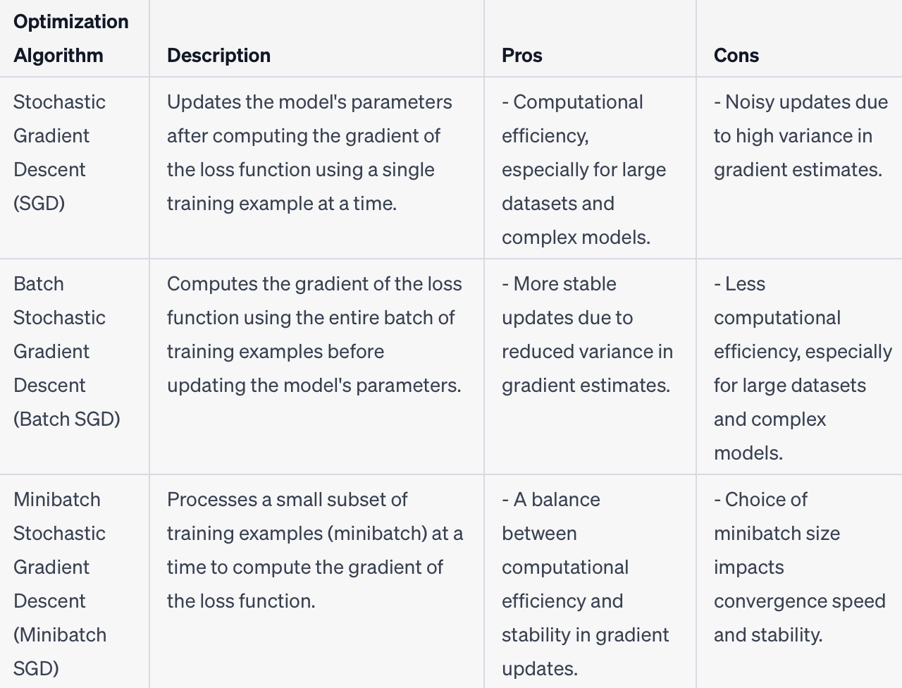
Batch SGD vs Minibatch SGD vs SGD
- The image below (source) shows the illustrated depiction of SGD and how it tries to find the local optima.
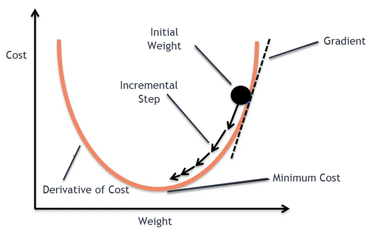
- Stochastic Gradient Descent (SGD):
- In traditional SGD, the model parameters are updated after processing each individual training example.
- It randomly selects one training example at a time and computes the gradient of the loss function with respect to the parameters based on that single example.
- The model parameters are then updated using this gradient estimate, and the process is repeated for the next randomly selected example.
- SGD has the advantage of being computationally efficient, as it only requires processing one example at a time.
- However, the updates can be noisy and may result in slower convergence since the gradient estimate is based on a single example.
- Batch Stochastic Gradient Descent (Batch SGD):
- Batch SGD is a variation of SGD where instead of processing one example at a time, it processes a small batch of training examples simultaneously.
- The model computes the gradient of the loss function based on this batch of examples and updates the parameters accordingly.
- The batch size is typically chosen to be larger than one but smaller than the total number of training examples.
- Batch SGD provides a balance between the computational efficiency of SGD and the stability of traditional Batch Gradient Descent.
- It reduces the noise in the gradient estimates compared to SGD and can result in faster convergence.
- Batch SGD is commonly used in practice as it combines the benefits of efficient parallelization and more stable updates.
- Minibatch SGD:
- In minibatch SGD, instead of processing one training example (SGD) or a full batch of examples (Batch SGD) at a time, a small subset of training examples, called a minibatch, is processed.
- The minibatch size is typically larger than one but smaller than the total number of training examples. It is chosen based on the computational resources and the desired trade-off between computational efficiency and stability of updates.
- The model computes the gradient of the loss function based on the minibatch examples and updates the parameters accordingly.
- This process is repeated iteratively, with different minibatches sampled from the training data, until all examples have been processed (one pass over the entire dataset is called an epoch).
- Minibatch SGD provides a balance between the noisy updates of SGD and the stability of Batch SGD.
- It reduces the noise in the gradient estimates compared to SGD and allows for better utilization of parallel computation resources compared to Batch SGD.
- Minibatch SGD is widely used in practice as it offers a good compromise between computational efficiency and convergence stability.
Batch Inference vs Online Inference
- Batch Inference:
- Batch inference refers to the process of making predictions or running inference on a batch of input data simultaneously.
- In this approach, multiple input examples are processed together, typically in parallel, to obtain predictions in a batch-wise manner.
- Batch inference is suitable when there is a need to process a large volume of data efficiently, as it takes advantage of parallel processing and can leverage hardware optimizations.
- It is commonly used in scenarios where real-time predictions are not required, such as offline data processing, batch jobs, or situations where latency is not a critical factor.
- Online Inference:
- Online inference, also known as real-time inference or serving, refers to making predictions or running inference on individual or small batches of input data in real-time as they arrive.
- In this approach, predictions are generated for each input instance or a small group of instances as they come in, without waiting for a complete batch.
- Online inference is commonly used in applications where low latency is crucial, such as recommendation systems, chatbots, fraud detection, and other real-time prediction tasks.
- It requires efficient and responsive systems that can handle individual or small batches of requests quickly, often leveraging techniques like caching, load balancing, and efficient serving infrastructure.
Learning rate schedules
- “The amount that the weights are updated during training is referred to as the step size or the “learning rate.” Specifically, the learning rate is a configurable hyperparameter used in the training of neural networks that has a small positive value, often in the range between 0.0 and 1.0.” (source)
- The image below (source) depicts the effects of the learning rate depending on it’s value:
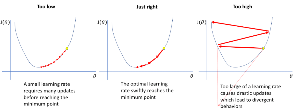
- “It is a scale of how big your model should update it’s weights and biases after every step. Normally, at the beginning of the training, you would want to gradients to update fast. Then, after a certain amount of step, you should decrease the learning rate.” (source)
- In the training process of a machine learning model, it is common to start with a relatively large learning rate to allow the model to quickly explore different areas of the parameter space and find a set of weights that yield reasonably good performance. This initial phase helps the model to escape from poor local optima.
- As the training progresses, the learning rate is typically reduced gradually or dynamically. This allows the model to make smaller adjustments to the weights, fine-tuning them to improve accuracy and converge towards the optimal solution. The smaller learning rate helps to make smaller, more precise updates and avoid overshooting the optimal weights.
- Constant learning rate:
- Constant learning rate involves using a fixed learning rate throughout the entire training process.
- This approach is commonly used when the dataset is relatively small and the learning problem is relatively simple.
- It can also be effective when the training data is consistent and the model is not prone to getting stuck in local optima.
- Constant learning rate is straightforward to implement and may converge quickly if the learning rate is appropriately set.
- Cosine decay:
- Cosine decay involves gradually reducing the learning rate over time following a cosine function.
- This approach is often employed when training deep neural networks or complex models with a large amount of data.
- Cosine decay helps the model to converge more smoothly by gradually reducing the learning rate.
- It allows the model to make smaller and more refined weight updates as the training progresses, which can improve the accuracy and generalization of the model.
- The choice of cosine decay can also be motivated by the desire to avoid overshooting the optimal solution and achieving better convergence.
- One such learning rate scheduling strategy can be, starting with an increased learning rate, followed by a constant hold, and then applying cosine decay, can be a valid approach in certain scenarios. Here’s a breakdown of each stage:
- Increasing the learning rate: Starting with a relatively high learning rate can help the model make larger initial weight updates and explore the parameter space more quickly. This can be beneficial in the early stages of training when the model needs to find a reasonable solution faster.
- Constant hold: After the initial increase, you may choose to keep the learning rate constant for a certain number of epochs or until a specific condition is met. This allows the model to stabilize and fine-tune its performance based on the knowledge gained during the initial high learning rate phase.
- Cosine decay: Once the model has reached a relatively stable state, applying cosine decay gradually reduces the learning rate over time. This schedule helps the model make smaller and more precise weight updates, allowing it to converge towards an optimal solution more smoothly. The cosine decay can prevent overshooting and improve the model’s accuracy and generalization.
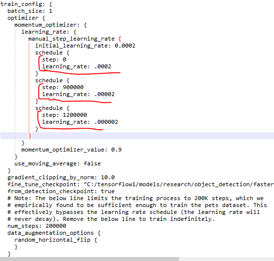
- When fine-tuning a pre-trained model, it is often recommended to lower the learning rate compared to the initial training phase. Fine-tuning involves taking a pre-trained model and further training it on a new task or dataset. Lowering the learning rate during this stage helps to ensure that the model does not make drastic updates to its parameters and instead focuses on refining its learned representations to better fit the new data.
- Use techniques such as learning rate schedules, grid search, or adaptive learning rate methods to find an optimal learning rate.
- Pros: An appropriate learning rate helps the model converge faster and achieve better performance.
- Cons: Choosing an incorrect learning rate can lead to slow convergence, instability, or suboptimal results.
What do you do when you have a low amount of data and large amount of features
- Data augmentation
- Data augmentation is a common technique used to address the problem of limited data by artificially increasing the size and diversity of the training dataset. It is particularly useful when the available data is limited but the number of features is relatively high. However, the effectiveness of data augmentation in such cases depends on the nature of the data and the specific task at hand.
Data augmentation involves applying a set of predefined transformations or perturbations to the existing data samples to create new, synthetic samples. These transformations introduce variations in the data while preserving the underlying patterns and characteristics. Some common data augmentation techniques include:
-
Geometric transformations: These involve applying operations such as rotations, translations, scaling, flipping, or cropping to the data. For example, in image data, you can rotate or flip images to create new training samples.
-
Noise injection: Adding random noise to the data can help create additional variations. For instance, in audio data, you can introduce background noise or random distortions.
-
Feature perturbations: Modifying specific features or attributes of the data can create diverse instances. For example, in text data, you can replace words with synonyms or introduce small modifications to sentence structure.
By augmenting the available data, you can effectively increase the size of the training dataset and expose the model to a broader range of variations, helping it generalize better to unseen data.
However, it’s important to note that data augmentation is not universally applicable and may not always be effective, especially if the available data is highly unique or if the specific domain or task requires a large amount of data for training. Additionally, the choice and extent of augmentation techniques should be carefully considered, as excessive or inappropriate augmentation can introduce artificial patterns or distortions that degrade model performance.
In summary, data augmentation can be a helpful strategy when dealing with low data and many features. It can expand the training dataset, introduce variations, and improve the generalization capability of models. However, its effectiveness depends on the nature of the data, the task, and the appropriate selection and application of augmentation techniques.
- Curse of dimensionality: The curse of dimensionality refers to the phenomenon where the data becomes more sparse and the distance between samples becomes less informative as the number of features increases. With limited data, this can result in difficulty in estimating reliable statistics, making it harder to identify meaningful patterns or relationships within the data.
- Dimensionality Reduction: Dimensionality reduction techniques are commonly used to address the curse of dimensionality and handle a large number of features. These techniques aim to reduce the feature space while retaining important information.
- Feature Selection: Selecting the most relevant features from the large feature set can help mitigate the impact of having low data. By focusing on the most informative features, you can reduce noise and improve the model’s ability to generalize.
- Feature Selection: This approach selects a subset of the original features based on certain criteria, such as their relevance to the target variable or their correlation with other features. Feature selection methods aim to retain the most informative features while discarding less important or redundant ones.
- Feature Extraction: In this approach, new features are derived from the original set of features using mathematical transformations. These new features, called latent variables or components, are constructed in such a way that they capture the essential information in the data. Principal Component Analysis (PCA) and Linear Discriminant Analysis (LDA) are examples of feature extraction techniques.
- Reduced Overfitting: High-dimensional feature spaces can increase the risk of overfitting, particularly when data is limited. By reducing the number of features, you can reduce the complexity of the model and improve its ability to generalize to unseen data.
- Improved Computational Efficiency: Having a large number of features can significantly increase the computational requirements for training and inference. Dimensionality reduction techniques help reduce the computational burden by reducing the feature space, making the model training process more efficient.
- Considerations:
- Data Quality: When dealing with limited data, it becomes crucial to ensure the quality and reliability of the available data. Noisy or inconsistent data can adversely impact the effectiveness of dimensionality reduction or feature selection techniques.
- Loss of Information: When reducing the dimensionality or selecting features, there is a risk of losing some important information or potentially relevant features. Careful consideration and evaluation are required to ensure that critical information is not discarded.
- Feature Engineering: In scenarios with low data, feature engineering becomes even more critical. By creating meaningful derived features or incorporating domain knowledge, you can enrich the dataset and provide more useful information to the model.
- Validation and Generalization: Due to the limited amount of data, it is essential to perform rigorous validation and testing to assess the model’s performance and generalization capability. Cross-validation and other evaluation techniques are important to ensure reliable results.
- Use models that can handle high-dimensional data efficiently, such as deep neural networks or ensemble methods.
- Pros: These models can capture complex patterns and relationships in the data, potentially leading to improved performance.
- Cons: High-dimensional data can increase the risk of overfitting, and the models may require more computational resources.
- Decorrelate features with Pearson correlation (linear correlation) and Spearman (monotonic, good with outliers) correlation can be used as measures to identify and remove decorrelated features when dealing with a large number of features and relatively less data. These correlation measures can provide insights into the linear or monotonic relationships between pairs of features.
- Here’s how you can use Pearson correlation or Spearman correlation for feature selection:
- Compute Correlation: Calculate the correlation coefficients between each pair of features in your dataset using either Pearson correlation (for continuous variables) or Spearman correlation (for ordinal or non-linear relationships).
- Set a Threshold: Determine a threshold value for correlation that defines the level of correlation beyond which features are considered strongly correlated. You can set a threshold based on domain knowledge or by observing the correlation distribution in your data.
- Identify Decorrelated Features: Identify pairs of features that have correlation coefficients below the threshold. These features are considered decorrelated or weakly correlated with each other.
- Remove Features: Remove one of the features from each pair of decorrelated features. This step helps in reducing redundancy and dimensionality in the feature space.
- By using Pearson or Spearman correlation to identify decorrelated features, you can effectively reduce the number of features in your dataset, eliminating those that are highly correlated with each other. This can help in mitigating the curse of dimensionality and improve the performance and interpretability of your models, especially when you have limited data.
- However, it’s important to note that correlation measures alone may not capture all types of relationships or interactions between features. It’s recommended to combine correlation-based feature selection with other techniques like domain knowledge, feature importance, or dimensionality reduction to ensure a comprehensive and effective feature engineering process.
- The choice between using Pearson correlation or Spearman correlation for feature selection depends on the nature of your data and the types of relationships you want to capture. Here’s a comparison between the two:
- Pearson Correlation:
- Measures the linear relationship between two continuous variables.
- Assumes that the relationship between variables is linear and follows a Gaussian distribution.
- Useful for identifying linear dependencies between features.
- Not suitable for capturing non-linear relationships or relationships involving ordinal variables.
- Spearman Correlation:
- Measures the monotonic relationship between variables, regardless of whether it is linear or not.
- Does not assume any specific distribution of data.
- Useful for identifying monotonic relationships or capturing non-linear dependencies between features.
- Can handle ordinal variables and is more robust to outliers.
- So, if you have continuous variables and want to capture linear relationships, Pearson correlation can be a good choice. On the other hand, if you have ordinal variables, non-linear relationships, or want a more robust measure, Spearman correlation is a better option.
- In some cases, it may be beneficial to use both correlation measures and compare the results. You can start with Pearson correlation to identify linear relationships and then use Spearman correlation to capture additional non-linear dependencies. This approach provides a more comprehensive understanding of the relationships between features.
- Ultimately, the choice of correlation measure depends on your specific data and the goals of your analysis. It’s recommended to consider the nature of your variables and the types of relationships you expect to find when deciding which correlation measure to use for feature selection.
Sample size
- Sample size refers to the number of data points or observations in the entire dataset. It represents the total amount of data available for training, validation, and testing. The sample size is a characteristic of the dataset itself and remains fixed throughout the training process.
- Population size: Consider the size of the population you are trying to make inferences about. If the population is small, you may need a larger sample size to obtain reliable estimates. Conversely, if the population is large, a smaller sample size might be sufficient.
- Desired level of precision: Determine the level of precision or margin of error that you are willing to tolerate in your estimates. A smaller margin of error requires a larger sample size.
- Confidence level: Specify the desired level of confidence in your estimates. Commonly used confidence levels are 95% or 99%. Higher confidence levels generally require larger sample sizes.
- Variability of the data: Consider the variability or dispersion of the data you are working with. If the data points are highly variable, you may need a larger sample size to capture the underlying patterns accurately.
- Statistical power: If you are conducting hypothesis tests or performing statistical analyses, you need to consider the statistical power of your study. Higher statistical power often necessitates a larger sample size to detect meaningful effects or differences.
- Available resources: Take into account the resources available to collect and analyze data. If there are limitations in terms of time, cost, or manpower, you may need to make trade-offs and choose a sample size that is feasible within those constraints.
- Prior research or pilot studies: If prior research or pilot studies have been conducted on a similar topic, they can provide insights into the expected effect sizes and variability, which can guide sample size determination.
- Nonlinear algorithms (ANN, SVN, Random Forest), which have the ability to learn complex relationships between input and output features, often require a larger amount of training data compared to linear algorithms. These nonlinear algorithms, such as random forests or artificial neural networks, are more flexible and have higher variance, meaning their predictions can vary based on the specific data used for training.
- For example, if a linear algorithm achieves good performance with a few hundred examples per class, a nonlinear algorithm may require several thousand examples per class to achieve similar performance. Deep learning methods, a type of nonlinear algorithm, can benefit from even larger amounts of data, as they have the potential to further improve their performance with more training examples
- Also note, more data never hurts!
How many attention layers do I need if I leverage a Transformer?
- The original Transformer model, as introduced in the “Attention is All You Need” paper by Vaswani et al., consists of six identical layers for both the encoder and decoder. However, this is not a strict rule, and the number of layers can be adjusted based on the requirements of the task.
- In general, increasing the number of attention layers can enhance the model’s capacity to capture complex patterns and dependencies in the data. However, a higher number of layers also increases computational requirements and may lead to overfitting if the dataset is not sufficiently large.
- It is common to start with a smaller number of attention layers, such as 4-6 layers, and then incrementally increase or decrease the number based on empirical evaluation and performance on validation data. Ultimately, the optimal number of attention layers is determined through experimentation and careful tuning specific to the task at hand.
Data diversity
- Regular updates: As your application or problem domain evolves, it’s important to regularly update and expand your dataset to maintain diversity. New data sources can be added, and existing data can be refreshed to reflect changes in the target population.
Balancing data:
- Balancing data refers to adjusting the class distribution in a dataset to ensure that each class or category is represented fairly. This is often done when there is a significant class imbalance, meaning some classes have significantly fewer samples compared to others. Balancing the data can help prevent bias and improve the performance of machine learning models.
- Here are some common techniques for balancing data:
- Oversampling: Increase the number of samples in the minority class by randomly replicating existing samples or generating synthetic samples using techniques like SMOTE (Synthetic Minority Over-sampling Technique). This helps to create a more balanced representation of classes.
- Undersampling: Decrease the number of samples in the majority class by randomly removing instances. This method aims to reduce the dominance of the majority class and increase the influence of the minority class.
- Stratified Sampling: During the dataset splitting process (e.g., train-test split or cross-validation), ensure that the ratio of different classes remains consistent in each subset. This helps maintain the class distribution across the training and evaluation phases.
- Ensemble Methods: Utilize ensemble learning techniques that combine multiple models trained on balanced subsets of the data. Each model focuses on a different subset or variation of the data to capture diverse representations.
- Cost-sensitive Learning: Assign different costs or weights to different classes during model training. This gives higher importance to underrepresented classes, forcing the model to pay more attention to them.
- Data Augmentation: Generate additional samples by applying transformations or perturbations to existing data. This technique can help increase the number of samples in the minority class, providing more training data without collecting new data.
Params, Weights, and Features
- Features:
- Features are the individual measurable characteristics or attributes that describe the entities in a given problem. In a recommendation system, features represent properties or characteristics of users and items (movies in this case). Features can include genre, director, release year, actors, user demographics, previous movie ratings, and so on. These features provide quantitative or categorical information that helps to represent and differentiate the entities being considered.
- Weights:
- Weights are parameters associated with each feature in a machine learning model. These weights determine the relative importance or contribution of each feature towards the final prediction or output of the model. In a recommendation system, the weights associated with features represent the significance or influence of those features in determining user preferences or item recommendations.
- During the training process, the model learns these weights by adjusting their values based on the input data and the desired output. The objective is to find the optimal combination of feature weights that minimize the prediction error or loss function.
- In a recommendation system using collaborative filtering, the weights associated with user features indicate how much importance is given to each feature in capturing user preferences. Similarly, the weights associated with movie features indicate the significance of each feature in representing the characteristics of movies. By learning and updating these weights, the model can capture the relationships and patterns between features and make accurate predictions or recommendations.
- Assume we have the following simplified movie recommendation model with the following parameters:
- User-Feature Matrix Parameters:
- Each user is represented by a feature vector capturing their preferences across different movie genres (comedy, action, romance).
- For example, let’s say we have User 1 with the following feature vector: [0.8, 0.2, 0.6].
- The associated parameters for User 1’s feature vector could be: [1.2, 0.9, 0.6].
- These parameters represent the weights or preferences of User 1 towards comedy, action, and romance genres, respectively.
- Movie-Feature Matrix Parameters:
- Each movie is represented by a feature vector describing its attributes, such as genre, director, and actors.
- Let’s consider a movie, Movie A, with the following feature vector: [0.5, 0.7, 0.9].
- The associated parameters for Movie A’s feature vector could be: [0.9, 0.5, 1.0].
- These parameters represent the weights or importance of each feature for Movie A, such as the significance of genre, director, and actors in determining its characteristics.
- During the training phase, these parameters are learned by adjusting their values to minimize the prediction error or loss. The model updates the parameters based on user ratings or preferences for movies and iteratively refines them to improve the recommendation accuracy.
- Once the parameters are learned, the model uses them to make personalized recommendations. For example, the model may calculate the similarity between User 1’s feature vector and the feature vectors of unseen movies, combining the associated parameters to predict the user’s rating for each movie. Based on these predictions, the model can recommend the top-rated movies to User 1.
Vanishing Gradients
- The vanishing gradient problem occurs when the gradients used to update the weights during backpropagation diminish exponentially as they propagate through deep layers of a neural network. This can make it difficult for the network to learn and update the weights of early layers effectively.
- When gradients become extremely small, the learning process slows down, and the network may struggle to converge or learn useful representations. The issue commonly arises in deep networks with many layers, such as recurrent neural networks (RNNs) or deep feedforward networks.
- To mitigate the vanishing gradient problem, various techniques have been developed, including:
- Activation functions: Replacing the sigmoid or hyperbolic tangent activation functions, which have a limited range of derivatives, with activation functions like ReLU (Rectified Linear Unit) that do not suffer from vanishing gradients.
- Weight initialization: Properly initializing the weights of the network, such as using techniques like Xavier or He initialization, to ensure that the gradients neither vanish nor explode during backpropagation.
- Gradient clipping: Limiting the magnitude of gradients during training to prevent them from becoming too large or too small.
Residual Connections/ Skip Connections
- Residual connections, also known as skip connections, are a technique introduced in the “Deep Residual Learning for Image Recognition” paper by He et al. (2015). They address the problem of information degradation or loss in deep neural networks.
- In a residual connection, the output of one layer (or a group of layers) is directly connected to the input of a subsequent layer. This creates a “shortcut” path that bypasses some of the layers. The key idea is to enable the network to learn residual functions that capture the difference between the desired output and the current representation.
- By allowing the network to learn residual functions, the gradients have a shorter path to propagate through the network during backpropagation. This helps in mitigating the vanishing gradient problem and facilitates the training of very deep networks.
- Residual connections have proven effective in improving the training and performance of deep neural networks, particularly in tasks such as image recognition, object detection, and natural language processing.
Methods to assess the quality and suitability of a model architecture
- Validation metrics: Measure the performance of the model on a validation dataset using appropriate evaluation metrics. The choice of metrics depends on the problem at hand, such as accuracy, precision, recall, F1 score, mean squared error (MSE), or mean absolute error (MAE). Compare these metrics with baseline models or industry standards to gauge the model’s effectiveness.
- Learning curves: Plot the learning curves to assess the convergence and performance of the model during training. Learning curves depict the model’s training and validation performance as the number of training iterations or epochs increases. A well-performing architecture should show convergence with both training and validation metrics improving over time.
- Cross-validation: Employ cross-validation techniques, such as k-fold cross-validation, to assess the model’s generalization performance. This involves splitting the data into multiple subsets and training the model on different combinations of training and validation sets. By averaging the performance across these iterations, you can obtain a more reliable estimate of the model’s performance.
- Overfitting and underfitting analysis: Check for signs of overfitting or underfitting. Overfitting occurs when the model performs well on the training data but poorly on unseen data, while underfitting implies the model’s inability to capture the underlying patterns in the data. Analyze the learning curves, validation metrics, and perform model diagnostics to identify these issues.
- Model complexity: Assess the complexity of the architecture and consider whether it aligns with the problem’s complexity. Very simple architectures may underfit the data, while overly complex architectures may overfit or be computationally inefficient. Strive for a balance by considering the problem’s complexity, available data, and computational resources.
- Comparative analysis: Compare your model’s performance with other state-of-the-art models or benchmark datasets in the field. This helps you understand if your architecture is achieving competitive or superior results. Participating in machine learning competitions or referring to literature can provide insights into the expected performance of different architectures.
- Real-world evaluation: Deploy the model in a real-world setting and evaluate its performance under practical conditions. Monitor key performance indicators (KPIs) and collect feedback from users or stakeholders. This allows you to assess how well the architecture addresses the specific needs and requirements of the application.
- Interpretability and explainability: Evaluate the interpretability and explainability of the model. Complex architectures may provide accurate predictions but lack transparency, making it challenging to understand the reasoning behind the model’s decisions. Ensuring a balance between model complexity and interpretability is crucial, especially in domains where explainability is essential.
Generate Embeddings
- TF-IDF (Term Frequency-Inverse Document Frequency):
- TF-IDF is a popular technique used for text-based recommender systems. It represents the importance of a term (word) in a document within a corpus. Here’s how it works:
- Corpus Preparation: Collect a corpus of textual data, such as product descriptions, user reviews, or item attributes.
- Text Preprocessing: Clean the text data by removing punctuation, stopwords, and applying techniques like stemming or lemmatization.
- Term Frequency (TF): Calculate the frequency of each term (word) in each document (item) within the corpus. This represents how often a term appears in a document.
- Inverse Document Frequency (IDF): Measure the rarity of each term across the entire corpus. This is done by calculating the logarithm of the inverse of the term’s document frequency (number of documents containing the term divided by the total number of documents).
- TF-IDF Calculation: Multiply the term frequency (TF) with the inverse document frequency (IDF) to obtain the TF-IDF score for each term in each document. This score represents the importance of the term in the document compared to its frequency in the corpus.
- Embedding Representation: Treat each document (item) as a vector, where each dimension corresponds to a term in the corpus. The TF-IDF score of a term in a document becomes the value in the corresponding dimension of the vector. These vectors serve as embeddings for the documents.
- TF (Term Frequency) helps capture the importance of a term within a specific movie description. It indicates how frequently a term appears in the movie’s content and helps identify the prominent themes or topics within the description. High TF values for certain terms suggest their significance in describing the movie.
- However, TF alone may not be sufficient to differentiate between common terms and those that are truly informative or distinctive. This is where IDF (Inverse Document Frequency) comes into play. IDF measures the rarity or uniqueness of a term across the entire movie corpus. It helps identify terms that are less common across movies but hold more discriminative power.
- By combining TF and IDF through the TF-IDF approach, the resulting scores reflect both the local importance of terms within a movie’s description (TF) and the global distinctiveness of those terms across the movie collection (IDF). This allows the recommendation system to highlight terms that are both prominent within a movie and unique compared to other movies, enabling more accurate content-based filtering.
- BM-25
- While both BM25 and TF-IDF are term weighting schemes used in information retrieval and text mining, they have some fundamental differences in how they calculate the importance or relevance of terms in a document.
- Calculation:
- TF-IDF (Term Frequency-Inverse Document Frequency) calculates the weight of a term based on its frequency within a document (TF) and its rarity across the entire document collection (IDF).
- BM25 (Best Match 25) also takes into account the term frequency within a document but uses a more sophisticated scoring function that considers factors like document length, average document length, and term frequency in the entire collection.
- Document Length:
- TF-IDF treats all documents as having equal length and does not explicitly account for differences in document length.
- BM25 incorporates the document length by penalizing the weight of terms based on the document length. Longer documents tend to have higher term frequencies, so BM25 compensates for this effect.
- Term Frequency Saturation:
- TF-IDF can suffer from term frequency saturation, where the importance of a term plateaus after a certain frequency threshold.
- BM25 addresses this issue by using a term frequency saturation function that prevents excessive term weight for high frequencies.
- Word Embeddings:
- Word embeddings capture the semantic meaning of words by representing them as dense, low-dimensional vectors. These embeddings are trained using neural network models, such as Word2Vec, GloVe, or FastText, on large corpora. Here’s a general process:
- Corpus Preparation: Gather a large corpus of text data, such as news articles, social media posts, or web documents.
- Tokenization: Split the text into individual words or subword units, known as tokens.
- Neural Network Training: Train a neural network model, such as Word2Vec, on the corpus. This model learns to predict the context (surrounding words) of a given word or vice versa.
- Embedding Extraction: Extract the learned weights from the trained model for each word. These weights form the word embeddings, where each word is represented by a dense vector.
- Pre-trained Embeddings: Alternatively, you can use pre-trained word embeddings that are trained on large external corpora, such as Google’s Word2Vec or Stanford’s GloVe. These pre-trained embeddings can be directly used in recommender systems without training on a specific corpus.
- Collaborative Filtering Embeddings:
- Collaborative filtering techniques consider user-item interactions to generate embeddings. Two common approaches are:
- Matrix Factorization: Factorize a user-item interaction matrix into lower-dimensional matrices representing user and item embeddings. The latent factors capture the underlying preferences or characteristics of users and items.
- Neural Collaborative Filtering: Utilize neural networks, such as Multi-Layer Perceptrons (MLPs) or Deep Neural Networks (DNNs), to learn user and item embeddings from interaction data. These embeddings can capture complex patterns and non-linear relationships.
- Hybrid Approaches:
- Hybrid recommender systems combine multiple types of embeddings to leverage both content and collaborative information. These embeddings can be concatenated, combined using weighted averages, or passed through additional layers to learn a joint representation.
- The choice of embedding method depends on the nature of the data and the specific goals of the recommender system. It is common to experiment with different approaches and evaluate their performance using metrics like precision, recall, or mean average precision (MAP
import pandas as pd
from scipy.sparse import csr_matrix
from sklearn.decomposition import TruncatedSVD

# Load the movie ratings data
ratings_data = pd.read_csv("ratings.csv")

# Create a sparse user-item matrix
user_item_matrix = ratings_data.pivot(index="user_id", columns="movie_id", values="rating").fillna(0)
sparse_matrix = csr_matrix(user_item_matrix.values)

# Apply Singular Value Decomposition (SVD)
svd = TruncatedSVD(n_components=100)
movie_embeddings = svd.fit_transform(sparse_matrix)

# Print the movie embeddings
print(movie_embeddings)
Multicollinearity
- Multicollinearity refers to the high correlation between input features in a dataset, which can adversely affect the performance of machine learning models. To identify multicollinearity, one can calculate the Pearson correlation coefficient or the Spearman correlation coefficient between the input features. The Pearson correlation coefficient measures the linear relationship between variables, while the Spearman correlation coefficient assesses the monotonic relationship between variables.
- Creating a heatmap by visualizing the correlation coefficients of input features can effectively reveal multicollinearity. In the heatmap, lighter colors indicate a high correlation, while darker colors indicate a low correlation.
- To mitigate multicollinearity, one approach is to employ Principal Component Analysis (PCA) as a data preprocessing step. PCA leverages the existing correlations among input features to combine them into a new set of uncorrelated features. By applying PCA, multicollinearity can be automatically addressed. After PCA transformation, a new heatmap can be generated to confirm the reduced correlation among the transformed features.
- For a practical demonstration of removing multicollinearity using PCA, you may refer to the article “How do you apply PCA to Logistic Regression to remove Multicollinearity?” to gain hands-on experience in its application.
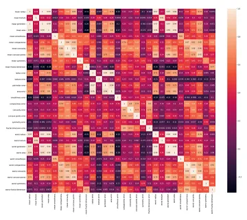
- (Source image)
Randomness
- Randomness plays a role in machine learning models, and the random state is a hyperparameter used to control the randomness within these models. By using an integer value for the random state, we can ensure consistent results across different executions. However, relying solely on a single random state can be risky because it can significantly affect the model’s performance.
- For instance, consider the train_test_split() function, which splits a dataset into training and testing sets. The random_state hyperparameter in this function determines the shuffling process prior to the split. Depending on the random state value, different train and test sets will be generated, and the model’s performance is highly influenced by these sets.
- To illustrate this, let’s look at the root mean squared error (RMSE) scores obtained from three linear regression models, where only the random state value in the train_test_split() function was changed:
- Random state = 0 → RMSE: 909.81
- Random state = 35 → RMSE: 794.15
- Random state = 42 → RMSE: 824.33
- As observed, the RMSE values vary significantly depending on the random state.
- To mitigate this issue, it is recommended to run the model multiple times with different random state values and calculate the average RMSE score. However, performing this manually can be tedious. Instead, cross-validation techniques can be employed to automate this process and obtain a more reliable estimate of the model’s performance.
- Relying on a single random state in machine learning models can yield inconsistent results, and it is advisable to leverage cross-validation methods to mitigate this issue.
Data leaks
- Data leakage occurs when preprocessing and transforming data, leading to biased and unreliable results. Two common scenarios where data leakage can occur are during feature standardization and when applying transformations to the data.
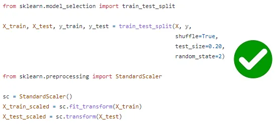
- In the case of feature standardization, data leakage happens when the entire dataset is standardized before splitting into training and test sets. This is problematic because the test set, which is derived from the full dataset, is used to calculate the mean and standard deviation for standardization. To prevent data leakage, it is recommended to perform feature standardization separately on the training and test sets after the data split.
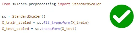
- Similarly, data leakage can occur when applying transformations to the data, such as using functions like StandardScaler or PCA. If the fit() method of these functions is called twice, once on the training set and again on the test set, new values are computed based on the test set, leading to biased results. To avoid data leakage, it is essential to call the fit() method only on the training set.
- By addressing these issues and avoiding data leakage, we can ensure the integrity and reliability of machine learning models.
- Data leakage can compromise the accuracy and generalizability of machine learning models. It is crucial to be cautious during preprocessing and transformation steps to prevent unintentional data leakage. By adhering to best practices and following proper procedures, we can minimize the risk of data leakage and obtain more robust and trustworthy results.
Underfitting
- Underfitting occurs when a model is too simple and fails to learn essential patterns in the training data. It results in poor performance on both the training data and new, unseen data. Underfitting can be identified by analyzing the learning curve, where the model’s performance remains consistently low.
- To avoid underfitting, the following techniques can be employed:
- Increase the complexity of the model.
- Increase the number of input features.
- Allow the model to train for a longer duration.
Overfitting
- Overfitting happens when a model is overly complex and tries to memorize the training data instead of learning underlying patterns. It performs well on the training data but fails to generalize to new, unseen data. Overfitting can be detected through the learning curve, which shows a significant gap between the performance on the training set and the performance on the validation or test set.
- To avoid overfitting, the following techniques can be employed:
- Increase the number of training examples.
- Use techniques such as feature selection, creating ensembles, dimensionality reduction, regularization, cross-validation, and early stopping.
- Utilize neural network-specific techniques like dropout, L1 and L2 regularization, early stopping, data augmentation, and noise regularization.
Not performing one-hot encoding when using categorical_crossentropy
- When utilizing the categorical_crossentropy loss function, it is essential to apply one-hot encoding to scalar value labels. Failure to do so will result in an error. The error arises because the categorical_crossentropy function expects one-hot encoded labels as input.
- To avoid this error, you can take the following measures:
- Use the sparse_categorical_crossentropy loss function instead of categorical_crossentropy. This function does not require one-hot encoding.
- Perform one-hot encoding on the labels and continue using the categorical_crossentropy loss function. One-hot encoding transforms scalar labels into n-element vectors, where n represents the number of classes. The to_categorical() function can be employed for this purpose.
- By adhering to these guidelines and ensuring proper one-hot encoding, you can effectively prevent errors and employ the categorical_crossentropy loss function accurately in your deep learning models.
Small dataset for complex algorithms
- Deep learning algorithms, such as neural networks, are primarily designed to excel when working with large datasets comprising millions or thousands of millions of training instances. In the case of small datasets, their performance is considerably limited.
- In fact, there are instances where deep learning algorithms perform even worse than conventional machine learning algorithms when applied to small datasets.
Failure to detect outliers in data
- Outliers are often present in real-world datasets, representing data points that deviate significantly from the majority of other data points. These outliers can be visually identified when plotting the data, as they appear distinctly separate from the rest.
- Methods for outlier detection:
- Z-Score or Standard Deviation Method: This method calculates the z-score for each data point based on its deviation from the mean and standard deviation of the dataset. Points with a z-score above a certain threshold (e.g., 3) are considered outliers.
- Several techniques can be employed to detect outliers, including:
- IQR-based detection
- Elliptic envelope
- Isolation forest
- One-class SVM
- Local outlier factor (LOF)
- Handling outliers:
- When dealing with outliers, it is crucial to carefully consider their significance. Simply removing outliers without understanding their underlying story is not recommended. If an outlier carries valuable information relevant to the problem at hand, it should be retained and accounted for in subsequent analysis. However, outliers resulting from data collection errors can be safely removed. Neglecting to address unnecessary outliers can introduce bias to the model and potentially lead to the omission of important patterns within the data.
Failure to verify model assumptions
- When constructing models, we often work under specific assumptions. These assumptions serve as the foundation for accurate predictions, provided they are not violated. Therefore, it is crucial to validate the underlying assumptions once the model is built.
- Examples of validating model assumptions:
- Normality assumption in linear regression: One assumption is that the residuals (the differences between observed and predicted values) in a linear regression model follow a normal distribution with a mean of zero and a fixed standard deviation. To verify this, we can create a histogram of the residuals and ensure they approximate a normal distribution. Additionally, calculating the mean of the residuals and confirming its proximity to zero reinforces this assumption.
- Histogram depicting the distribution of residuals (Image by author)
- Independence assumption in linear regression: Another assumption is that the residuals in a linear regression model are uncorrelated or independent. We can verify this assumption by generating a residual plot, examining the pattern of the residuals to ensure no systematic correlation exists between them.
Failure to utilize a validation set for hyperparameter tuning
- In the process of hyperparameter tuning, it is essential to employ a distinct dataset known as the validation set, in addition to the training and testing datasets. Utilizing the same training data for hyperparameter tuning can result in data leakage, undermining the model’s ability to generalize to new, unseen data.
- To ensure an effective approach, the training set is utilized for fitting the model parameters, the validation set is dedicated to fine-tuning the model’s hyperparameters, and the test set is employed to evaluate the model’s performance. By adhering to this methodology, we can enhance the model’s overall effectiveness and robustness.
- Using a validation set for hyperparameter tuning is crucial for several reasons:
- Preventing Overfitting: Hyperparameter tuning involves adjusting the settings of the model to optimize its performance. Without a validation set, tuning is performed on the same data used for training, which can lead to overfitting. Overfitting occurs when the model becomes too specific to the training data and performs poorly on new, unseen data. By utilizing a separate validation set, we can assess the model’s performance on unseen data and make more informed decisions during hyperparameter tuning.
- Evaluating Generalization: The primary goal of machine learning is to build models that can generalize well to unseen data. A validation set allows us to evaluate the model’s performance on data it hasn’t encountered during training. By tuning the hyperparameters based on the validation set’s performance, we increase the chances of the model’s ability to generalize and perform well on new data.
- Avoiding Data Leakage: Data leakage refers to situations where information from the test or validation set unintentionally leaks into the training process, leading to overly optimistic performance estimates. If the same data is used for both training and hyperparameter tuning, the model can indirectly “learn” about the validation data and bias the tuning process. By using a separate validation set, we ensure that the tuning process remains independent and unbiased.
Less data for training
- Allocating an adequate amount of data for the training set is crucial for effective model learning and generalization. The following points highlight the importance of allocating a sufficient portion of the dataset for training:
- Enhanced Learning: A larger training set allows the model to access a wider range of examples, enabling it to capture diverse patterns and relationships present in the data. With more data, the model can learn more robust representations and make better predictions. Therefore, it is advisable to allocate a significant portion of the data for training.
- Generalization Improvement: A well-trained model should be capable of performing well on unseen data. By providing a substantial training set, the model has a better chance of learning the underlying patterns that generalize to new instances. This helps in improving the model’s ability to make accurate predictions on real-world data.
- Additionally, here are some guidelines for choosing the training set size:
- For small datasets containing hundreds or thousands of samples, it is recommended to allocate approximately 70%-80% of the data for training. This ensures that the model has access to a sufficient number of examples to learn meaningful patterns and relationships.
- For large datasets with millions or billions of samples, a higher allocation, such as 96%-98% of the data, can be used for training. The abundance of data allows the model to effectively capture complex patterns and make accurate predictions.
- Remember that the specific allocation percentages may vary based on the nature of the dataset and the specific problem at hand. It is important to strike a balance between the training set size and the availability of data for validation and testing purposes.
- By allocating a substantial amount of data for the training set, we provide the model with ample opportunities to learn and generalize effectively, leading to improved performance on unseen data.
Accuracy metric used to evaluate models with data imbalance
- When dealing with class imbalance, where one class has a significantly larger number of instances than the other, using accuracy as an evaluation metric can be misleading. It is important to consider the following points:
- Imbalanced Class Distribution: In datasets with class imbalance, the majority class dominates the overall distribution, while the minority class is underrepresented. For instance, in a spam email detection dataset, there may be 9900 instances of the “Not spam” class and only 100 instances of the “Spam” class.
- Accuracy Bias: Accuracy alone is not a reliable metric in the presence of class imbalance. A model trained on such data may achieve a high accuracy score by simply predicting the majority class (i.e., “Not spam”). However, this accuracy does not reflect the model’s performance in capturing the minority class (i.e., “Spam”).
- Failure to Capture Minority Class: Due to the imbalanced nature of the dataset, the model may struggle to learn the patterns and characteristics of the minority class. Consequently, it may perform poorly in predicting instances belonging to the minority class, leading to false negatives or misclassifications.
- To properly evaluate models with class imbalance, it is recommended to use evaluation metrics that provide a more comprehensive understanding of the model’s performance. Some commonly used metrics in this context include:
- Precision and Recall: Precision measures the proportion of correctly predicted positive instances (e.g., “Spam”) out of all instances predicted as positive. Recall, on the other hand, calculates the proportion of correctly predicted positive instances out of all actual positive instances. These metrics are more informative about the model’s performance on the minority class.
- F1-Score: The F1-score is the harmonic mean of precision and recall. It provides a balanced evaluation of the model’s performance by considering both precision and recall. This metric is useful for assessing models in imbalanced datasets.
- Area Under the Receiver Operating Characteristic Curve (AUC-ROC): The AUC-ROC score quantifies the model’s ability to discriminate between the classes across different classification thresholds. It provides a holistic view of the model’s performance, taking into account both true positive and false positive rates.
- By using these metrics, we can obtain a more accurate assessment of the model’s performance, specifically in capturing the minority class and mitigating the bias introduced by class imbalance.
Omitting data normalization
- Neglecting to normalize the input and output data can have adverse effects on the performance of neural networks.
- It is crucial to ensure that the data is distributed with a mean close to zero and a standard deviation of approximately one before feeding it into the network.
Using excessively large batch sizes
- Employing a very large batch size can hinder the model’s ability to generalize well and may negatively impact the accuracy during training.
- This is due to reduced stochasticity in the gradient descent process, which can prevent the network from effectively navigating the optimization landscape.
Neglecting to apply regularization techniques
- Regularization serves a dual purpose of preventing overfitting and aiding in handling noise and outliers in the data.
- For efficient and stable training, it is important to incorporate appropriate regularization techniques into the model.
Selecting an incorrect learning rate
- The choice of learning rate plays a critical role in training the network. An improper learning rate can make the training process challenging or even infeasible.
- It is essential to find an appropriate learning rate that facilitates effective convergence and avoids issues such as slow training or unstable optimization.
Using an incorrect activation function for the output layer
- Employing an inappropriate activation function for the output layer can result in the network failing to produce the desired range of values.
- For instance, using ReLU activation on the output layer may restrict the network to only positive output values. It is important to select an activation function that aligns with the desired output behavior.
Employing an excessively deep network or an incorrect number of hidden units
- Deeper networks are not always better, and using an incorrect number of hidden units can impede training progress. In some cases, a very small number of units may lack the capacity to express the desired objective, while an excessively large number of units can lead to slow and computationally intensive training, making it challenging to remove residual noise during the training process.
- Finding the right balance in terms of the depth of the network and the number of hidden units involves a combination of experimentation, analysis, and validation. Here are some approaches that can help in finding the optimal balance:
- Start with simpler architectures: It is often recommended to start with a simpler architecture and gradually increase its complexity. Begin with a shallow network and a moderate number of hidden units. Train and evaluate the model’s performance to establish a baseline.
- Evaluate performance on validation data: Use a separate validation dataset to assess the model’s performance as you modify its architecture. Monitor key performance metrics such as accuracy, loss, or other relevant metrics specific to your problem domain. This can provide insights into how the changes in architecture affect the model’s ability to generalize.
- Explore different architectures: Experiment with different network architectures, varying the depth and number of hidden units. Consider increasing the depth of the network gradually, adding more hidden units to specific layers, or even exploring different layer configurations (e.g., convolutional layers, recurrent layers). Evaluate each architecture on the validation set to compare their performance.
- Regularization techniques: Apply regularization techniques such as dropout, L1/L2 regularization, or batch normalization to control overfitting and improve generalization. Regularization can help prevent the network from becoming overly complex and reduce the risk of overfitting, especially when dealing with larger architectures.
- Cross-validation: Perform cross-validation, particularly when the dataset size is limited. This involves splitting the data into multiple folds, training the model on different combinations of training and validation sets, and evaluating its performance. Cross-validation helps in obtaining a more robust estimate of the model’s performance and can guide the selection of the optimal architecture.
- Consider computational constraints: Take into account the available computational resources and time constraints. Deep networks with a large number of parameters can be computationally expensive to train, especially with limited resources. Ensure that the chosen architecture strikes a balance between performance and computational feasibility.
- Domain expertise and intuition: Leverage your domain knowledge and intuition to guide the architectural choices. Consider the specific characteristics of your problem and the nature of the data. For example, in image processing tasks, convolutional neural networks (CNNs) are commonly used due to their ability to capture spatial features.
- Remember that finding the right balance is an iterative process. It may require several rounds of experimentation, evaluation, and fine-tuning. It is important to assess the trade-offs between model complexity, computational requirements, and the desired performance on both training and validation/test data.
Data Drift And Semantic Shift
- Data drift refers to the phenomenon where the statistical properties of the data change over time, leading to a discrepancy between the training data and the real-time data the model encounters during deployment. Ignoring data drift can significantly degrade the performance and accuracy of AI models.
- To address data shift and semantic shift, organizations should consider the following practices:
- Continuous data monitoring: Implement a robust data monitoring system to track and analyze changes in the input data distribution. This involves regularly collecting and analyzing new data points to identify any significant shifts or deviations from the training data. Data monitoring can be done through statistical analysis, visualization techniques, or by using specialized tools and platforms.
- Data preprocessing and feature engineering: As new data streams in, it is crucial to preprocess and engineer features to ensure compatibility with the existing model. This may involve adapting existing preprocessing steps or introducing new techniques to handle changes in data formats, data types, or feature distributions.
- Retraining and updating models: When significant data drift is detected, it may be necessary to retrain or update the AI models to capture the evolving patterns in the data. This can be done by incorporating new labeled data into the training set or by using techniques such as transfer learning, where a pre-trained model is fine-tuned with the new data. Regular model reevaluation and refinement are essential to ensure models remain accurate and effective over time.
- Ensemble modeling: Ensemble modeling involves combining predictions from multiple models to enhance performance and robustness. By training and maintaining multiple models with different architectures or trained on different datasets, organizations can leverage diversity in model predictions to mitigate the impact of data drift.
- Feedback loops and user feedback: Establish feedback mechanisms that allow users or domain experts to provide insights, flag issues, and highlight areas where the model’s predictions may be deviating from the expected behavior. User feedback can provide valuable information for understanding data shift and addressing potential problems in model performance.
- Human-in-the-loop approach: Incorporate human expertise and intervention into the model’s decision-making process. Human reviewers or validators can play a role in ensuring the model’s predictions align with domain knowledge and handle cases where the model’s performance may be affected by data drift.
- Regular model audits and performance evaluations: Conduct periodic audits and evaluations of the model’s performance to identify any degradation or deviation from the desired accuracy. This can involve comparing model predictions with ground truth data, conducting A/B testing, or employing external evaluation techniques.
- Data governance and documentation: Implement robust data governance practices to track and document changes in data sources, transformations, and preprocessing steps. Maintaining a comprehensive record of data shifts and the corresponding model updates can aid in understanding the impact of data drift and ensuring transparency and accountability.
- There are several techniques commonly used to detect data drift in machine learning applications. I’ll explain a few of them:
-
Statistical Measures: Statistical measures can be used to detect changes in the distribution of data. This can include measures like mean, standard deviation, skewness, and kurtosis. By comparing these measures between different time periods or datasets, you can identify potential drift.
-
Drift Detection Algorithms: There are specific algorithms designed to detect data drift, such as the Drift Detection Method (DDM) and the Page-Hinkley test. These algorithms monitor the incoming data stream and look for statistically significant changes that indicate drift.
-
Hypothesis Testing: Hypothesis testing can be used to formally test whether the distribution of data has changed. Techniques like the Kolmogorov-Smirnov test or the chi-square test can be applied to compare the distributions of different datasets or time periods.
-
Monitoring Performance Metrics: Monitoring performance metrics of your machine learning model can also help detect data drift. By regularly evaluating the model’s performance on new data and comparing it to a baseline, you can identify when the model’s accuracy or other metrics start to decline significantly, indicating potential drift.
-
Model Drift Detection: Another approach is to monitor the drift in the model’s predictions directly. This can involve comparing the model’s predictions on new data to the ground truth labels or comparing the predictions of multiple models trained on different time periods or datasets.
It’s worth noting that no single technique is universally applicable in all scenarios, and the choice of method depends on the specific problem, available resources, and data characteristics. It’s often beneficial to combine multiple techniques to gain a more comprehensive understanding of data drift in machine learning applications.
- One common technique to detect data drift in machine learning applications is to compare the statistical properties of different data distributions over time. Here are a few techniques commonly used to detect data drift:
-
Monitoring Descriptive Statistics: Track key descriptive statistics, such as mean, standard deviation, or skewness, for relevant features in the dataset. Any significant changes in these statistics over time can indicate data drift.
-
Statistical Hypothesis Testing: Apply statistical tests to compare the distributions of different datasets. For example, you can use the Kolmogorov-Smirnov test, the Anderson-Darling test, or the Mann-Whitney U test to check if the data distributions are significantly different.
-
Drift Detection Methods: There are specific drift detection methods designed to identify changes in data distributions. Examples include the Drift Detection Method (DDM), the Page-Hinkley Test, the Sequential Probability Ratio Test (SPRT), and the Cumulative Sum (CUSUM) algorithm. These methods analyze incoming data incrementally and raise an alarm when a significant change is detected.
-
Machine Learning Model Monitoring: Track the performance of your machine learning models over time. Monitor metrics such as accuracy, precision, recall, or the area under the ROC curve (AUC-ROC). A significant drop in performance can indicate a drift in the data.
-
Feature Importance Analysis: Use feature importance techniques to assess which features have the most impact on model predictions. If the importance of certain features changes significantly over time, it suggests that those features may be drifting.
-
Domain Expert Knowledge: Incorporate domain expertise to identify potential sources of data drift. Experts can provide insights into changes in the data-generating process, external factors impacting the data, or shifts in user behavior that might affect the data distribution.
It’s important to note that data drift detection is an ongoing process, and there is no one-size-fits-all solution. Different techniques may be more suitable depending on the specific problem, the nature of the data, and the available resources. Combining multiple methods and continuously monitoring the data can help you identify and address data drift in machine learning applications.
Continuous Training Continuous Testing - remove data drift
- Data validation
- You need to monitor the data your model is ingesting in the upstream pipeline because ‘garbage in, garbage out’. Your model is sensitive to the input data it receives. If there’s a change in the statistical distribution of the trained data from the data in production, model performance will decline significantly.
- Major data quality issues to monitor:
- Data schema
- Before retraining your model, you need to validate that your input data complies with the expected schema upstream. This means that your downstream pipeline steps, including data processing and model training, should be exactly the same with the schema from the production data. You can make use of the Python Assertion method to validate your schema against the expected schema.
- If the schema doesn’t comply with the expected schema, the data science team can update the pipeline to handle these changes. This might mean retraining a new model from scratch to accommodate the new features, or it might only mean renaming the features.
- Data Drift
- Another data quality issue to watch out for is data drift. This simply means that there’s a change in the statistical properties of data.
- Model validation
- After successfully validating your data pipeline, you need to also validate your model pipeline. The model pipeline is validated before it’s deployed to production.-
- Model validation steps include:
- Testing model performance using an adopted metric with a chosen threshold. It’s important to monitor model performance in production. If it falls below the threshold, a retraining job can be triggered. The re-trained model can be tested.
- Model metadata and versioning. Monitoring what works well in production is important. After running a series of experiments when retraining your machine learning model, you need to save all the model metadata for reproducibility. Your retraining pipeline should log different model versions and metadata to a metadata store alongside model performance metrics. A very good tool for managing your model metadata is neptune.ai.
- Concerted adversaries. As the field of machine learning is evolving, businesses are beginning to employ machine learning applications as the central decision maker. It’s important to monitor the security of models in production. Some machine learning models, like credit risk models, are susceptible to adversarial attacks. Fraudsters are always looking for different ways to trick a model poised with the task to identify suspicious credit card transactions.
- Model Infrastructure. You also need to monitor your model infrastructure compatibility and consistency with the prediction service API before you deploy into production.
- What is Continuous Training?
- Continuous training is an aspect of machine learning operations that automatically and continuously retrains machine learning models to adapt to changes in the data before it is redeployed. The trigger for a re-build can be data change, model change, or code change.
- Why is continuous training important?
- We’re going to explore the reasons why you still need to change your model in production after spending so much time training and deploying it in the first place.
- Machine learning models get stale with time
- As soon as you deploy your machine learning model in production, the performance of your model degrades. This is because your model is sensitive to changes in the real world, and user behaviour keeps changing with time. Although all machine learning models decay, the speed of decay varies with time. This is mostly caused by data drift, concept drift, or both.
- Data drift (covariate shift) is a change in the statistical distribution of production data from the baseline data used to train or build the model. Data from real-time serving can drift from the baseline data due to:
- Changes in the real world,
- Training data not being a representation of the population,
- Data quality issues like outliers in the dataset.
- For example, if you built a model with temperature data collected from a sensor in Celsius degrees, but the unit changed to Fahrenheit – it means there’s been a change in your input data, so the data has drifted.
- How to monitor data drift in production
- The best approach to handling data drift is to continuously monitor your data with advanced MLOps tools instead of using traditional rule-based methods. Rule based methods, like calculating the data range or comparing data attributes to detect alien values, can be time-consuming and are susceptible to error.
- Steps you can take to detect data drift:
- Take advantage of the JS-Divergence algorithm to identify prediction drift in real-time model output and compare it with training data.
- Compare the data distribution from both upstream and downstream data to view the actual difference.
- As mentioned above, you can also take advantage of the Fiddler AI platform to monitor data drift in production.
- What is concept drift?
- Concept drift is a phenomenon where the statistical properties of the target variable you’re trying to predict changes over time. This means that the concept has changed but the model doesn’t know about the change.
- Concept drift happens when the original idea your model had about the target class changes. For example, you build a model to classify positive and negative sentiment of tweets around certain topics, and over time people’s sentiment about these topics changes. Tweets belonging to positive sentiment may evolve over time to be negative.
- In simple terms, the concept of sentiment analysis has drifted. Unfortunately, your model will keep predicting positive sentiments as negative sentiments.
how to debug when online and offline results are inconsistent
- One way to deal with the situation is to investigate the differences between the training and A/B testing. Here a couple of common differences:
- The modeling training process optimizes a machine learning loss function. A/B test optimizes a business value. The loss function and business value could diverge.
- Data distributions are different. The machine learning model is trained on older data. The A/B test is on newer data. The older and newer data come from different distributions.
- When facing inconsistencies between online and offline results in a machine learning system, it can be challenging to identify and resolve the underlying issues. Here are some approaches to debug such inconsistencies:
-
Data Discrepancies: Start by investigating any differences in the data used for offline training and online inference. Check if the data preprocessing steps, feature engineering, or data sampling techniques differ between the two environments. Look for variations in data sources, data collection processes, or data pipelines that might contribute to the inconsistencies.
-
Feature Drift: Analyze the feature distributions and monitor for feature drift over time. Changes in the feature distributions between offline and online data can impact model performance. Ensure that the feature extraction and transformation processes are consistent and aligned in both training and inference stages.
-
Model Versioning: Verify that the correct model versions are deployed for online inference. Check for any discrepancies between the model used during offline training and the model deployed in the online system. Ensure that the model serialization, deployment process, and any associated dependencies are consistent between offline and online environments.
-
Serving Infrastructure: Investigate the serving infrastructure and deployment pipeline for potential issues. Check for inconsistencies in model serving frameworks, deployment configurations, or server-side processing steps. Ensure that the serving infrastructure accurately reflects the offline training pipeline to minimize discrepancies.
-
Real-Time Factors: Consider real-time factors that might impact online results, such as network latency, system load, or external dependencies. Issues like network delays, timing differences in data availability, or fluctuating external factors can lead to inconsistencies. Monitor and measure these factors to identify any potential discrepancies.
-
Logging and Monitoring: Implement comprehensive logging and monitoring mechanisms in both offline and online systems. Log important metrics, predictions, and system events to trace the execution flow and identify any discrepancies. Utilize monitoring tools to track key performance indicators, model metrics, and system health in real-time.
-
A/B Testing: Conduct A/B testing experiments to compare different system configurations, models, or data preprocessing methods. By comparing the performance of different variants in controlled experiments, you can identify factors that contribute to inconsistencies and make data-driven decisions to address them.
Remember that debugging inconsistencies between offline and online results requires a systematic approach and thorough analysis. It may involve a combination of data analysis, system profiling, experimentation, and close collaboration between data scientists, engineers, and domain experts.
Regarding the question about the model file being very large, it could be caused by various factors:
- Model Architecture: If the model architecture is complex and contains many layers or parameters, it can contribute to a large model size. Techniques like wide and deep learning, which combine deep neural networks with wide linear models, can result in larger model sizes compared to simpler architectures.
- Embeddings or Feature Representations: If the model relies on extensive embeddings or high-dimensional feature representations, it can increase the size of the model file. Embeddings can capture rich information about users, businesses, or contextual features but can also lead to larger model sizes.
- Data and Model Complexity: The size of the model file can also be influenced by the size and complexity of the training data. If the dataset used for training is large, contains high-dimensional features, or has a high level of detail, it can contribute to a larger model size.
- Model Serialization and Storage: The serialization and storage format used for the model file can impact its size. Some serialization formats may introduce additional overhead or compression techniques that affect the file size.
-
To address the issue of a large model file, you can consider the following approaches:
- Model Compression: Apply model compression techniques such as pruning, quantization, or knowledge distillation to reduce the size of the model without significantly sacrificing performance. These techniques aim to remove redundant or less important parameters from the model.
- Transfer Learning: Utilize pre-trained models and transfer learning to leverage existing knowledge and reduce the need for training large models from scratch. Transfer learning allows you to build on pre-trained models and fine-tune them for specific tasks, potentially reducing the overall model size.
- Model Optimization: Optimize the model architecture and design to strike a balance between model complexity and performance. Consider using simpler architectures or alternative model architectures
What are some drawbacks of the Transformer?
- The runtime of Transformer architecture is quadratic in the length of the input sequence, which means it can be slow when processing long documents or taking characters as inputs. In other words, computing all pairs of interactions during self-attention means our computation grows quadratically with the sequence length, i.e., \(O(T^2 d)\), where \(T\) is the sequence length, and \(d\) is the dimensionality. Note that for recurrent models, it only grew linearly!
- Say, \(d = 1000\). So, for a single (shortish) sentence, \(T \leq 30 \Rightarrow T^{2} \leq 900 \Rightarrow T^2 d \approx 900K\). Note that in practice, we set a bound such as \(T=512\). Imagine working on long documents with \(T \geq 10,000\)!?
- Wouldn’t it be nice for Transformers if we didn’t have to compute pair-wise interactions between each word pair in the sentence? Recent studies such as:
- Synthesizer: Rethinking Self-Attention in Transformer Models
- Linformer: Self-Attention with Linear Complexity
- Rethinking Attention with Performers
- Big Bird: Transformers for Longer Sequences
- … show that decent performance levels can be achieved without computing interactions between all word-pairs (such as by approximating pair-wise attention).
- Compared to CNNs, the data appetite of transformers is obscenely high. CNNs are still sample efficient, which makes them great candidates for low-resource tasks. This is especially true for image/video generation tasks where an exceptionally large amount of data is needed, even for CNN architectures (and thus implies that Transformer architectures would have a ridiculously high data requirement). For example, the recent CLIP architecture by Radford et al. was trained with CNN-based ResNets as vision backbones (and not a ViT-like transformer architecture). While transformers do offer accuracy bumps once their data requirement is satisfied, CNNs offer a way to deliver decent accuracy performance in tasks where the amount of data available is not exceptionally high. Both architectures thus have their usecases.
- The runtime of the Transformer architecture is quadratic in the length of the input sequence. Computing attention over all word-pairs requires the number of edges in the graph to scale quadratically with the number of nodes, i.e., in an \(n\) word sentence, a Transformer would be doing computations over \(n^{2}\) pairs of words. This implies a large parameter count (implying high memory footprint) and thereby high computational complexity. More in the section on What Would We Like to Fix about the Transformer?
- High compute requirements has a negative impact on power and battery life requirements, especially for portable device targets.
- Overall, a transformer requires higher computational power, more data, power/battery life, and memory footprint, for it to offer better performance (in terms of say, accuracy) compared to its conventional competitors.
Why do we initialize weights randomly? / What if we initialize the weights with the same values?
- If all weights are initialized with the same values, all neurons in each layer give you the same outputs (and thus redundantly learn the same features) which implies the model will never learn. This is the reason that the weights are initialized with random numbers.
- Detailed explanation:
- The optimization algorithms we usually use for training neural networks are deterministic. Gradient descent, the most basic algorithm, that is a base for the more complicated ones, is defined in terms of partial derivatives
-
A partial derivative tells you how does the change of the optimized function is affected by the \(\theta_j\) parameter. If all the parameters are the same, they all have the same impact on the result, so will change by the same quantity. If you change all the parameters by the same value, they will keep being the same. In such a case, each neuron will be doing the same thing, they will be redundant and there would be no point in having multiple neurons. There is no point in wasting your compute repeating exactly the same operations multiple times. In other words, the model does not learn because error is propagated back through the weights in proportion to the values of the weights. This means that all hidden units connected directly to the output units will get identical error signals, and, since the weight changes depend on the error signals, the weights from those units to the output units will be the same.
-
When you initialize the neurons randomly, each of them will hopefully be evolving during the optimization in a different “direction”, they will be learning to detect different features from the data. You can think of early layers as of doing automatic feature engineering for you, by transforming the data, that are used by the final layer of the network. If all the learned features are the same, it would be a wasted effort.
-
The Lottery Ticket Hypothesis: Training Pruned Neural Networks by Frankle and Carbin explores the hypothesis that the big neural networks are so effective because randomly initializing multiple parameters helps our luck by drawing the lucky “lottery ticket” parameters that work well for the problem.
Describe learning rate schedule/annealing.
- Am optimizer is typically used with a learning rate schedule that involves a short warmup phase, a constant hold phase and an exponential decay phase. The decay/annealing is typically done using a cosine learning rate schedule over a number of cycles (Loshchilov & Hutter, 2016).
Explain mean/average in terms of attention.
- Averaging is equivalent to uniform attention.
What is convergence in k-means clustering?
- In case of \(k\)-means clustering, the word convergence means the algorithm has successfully completed clustering or grouping of data points in \(k\) number of clusters. The algorithm determines that it has grouped/clustered the data points into correct clusters if the centroids (\(k\) values) in the last two consequent iterations are same then the algorithm is said to have converged. However, in practice, people often use a less strict criteria for convergence, for e.g., the difference in the values of last two iterations needs to be less than a low threshold.
List some debug steps/reasons for your ML model underperforming on the test data.
- Insufficient quantity of training data: Machine learning algorithms need a large amount of data to be able to learn the underlying statistics from the data and work properly. Even for simple problems, the models will typically need thousands of examples.
- Nonrepresentative training data: In order for the model to generalize well, your training data should be representative of what is expected to be seen in the production. If the training data is nonrepresentative of the production data or is different this is known as data mismatch.
- Poor quality data: Since the learning models will use the data to learn the underlying pattern and statistics from it. It is critical that the data are rich in information and be of good quality. Having training data that are full of outliers, errors, noise, and missing data will decrease the ability of the model to learn from data, and then the model will act poorly on new data.
- Irrelevant features: As the famous quote says “garbage in, garbage out”. Your machine learning model will be only able to learn if the data contains relevant features and not too many irrelevant features.
- Overfitting the training data: Overfitting happens when the model is too complex relative to the size of the data and its quality, which will result in learning more about the pattern in the noise of the data or very specific patterns in the data which the model will not be able to generalize for new instances.
- Underfitting the training data: Underfitting is the opposite of overfitting, the model is too simple to learn any of the patterns in the training data. This could be known when the training error is large and also the validation and test error is large.
Popular machine learning models: Pros and Cons.
Linear Regression
Pros
- Simple to implement and efficient to train.
- Overfitting can be reduced by regularization.
- Performs well when the dataset is linearly separable.
Cons
- Assumes that the data is independent which is rare in real life.
- Prone to noise and overfitting.
- Sensitive to outliers.
Logistic Regression
Pros
- Less prone to over-fitting but it can overfit in high dimensional datasets.
- Efficient when the dataset has features that are linearly separable.
- Easy to implement and efficient to train.
Cons
- Should not be used when the number of observations are lesser than the number of features.
- Assumption of linearity which is rare in practice.
- Can only be used to predict discrete functions.
Support Vector Machines
Pros
- Good at high dimensional data.
- Can work on small dataset.
- Can solve non-linear problems.
Cons
- Inefficient on large data.
- Requires picking the right kernal.
Decision Trees
- Decision Trees can be used for both classication and regression.
- For classification, you can simply return the majority vote of the trees.
- For regression, you can return the averaged values of the trees.
Pros
- Can solve non-linear problems.
- Can work on high-dimensional data with excellent accuracy.
- Easy to visualize and explain.
Cons
- Overfitting. Might be resolved by random forest.
- A small change in the data can lead to a large change in the structure of the optimal decision tree.
- Calculations can get very complex.
k-Nearest Neighbor
- k-Nearest Neighbor (kNN) can be used for both classification and regression.
- For classification, you can simply return the majority vote of the nearest neighbors.
- For regression, you can return the averaged values of the nearest neighbors.
Pros
- Can make predictions without training.
- Time complexity is \(O(n)\).
- Can be used for both classification and regression.
Cons
- Does not work well with large dataset.
- Sensitive to noisy data, missing values and outliers.
- Need feature scaling.
- Choose the correct \(K\) value.
k-Means Clustering
- k-Means Clustering (kMC) is a classifier.
Pros
- Simple to implement.
- Scales to large data sets.
- Guarantees convergence.
- Easily adapts to new examples.
- Generalizes to clusters of different shapes and sizes.
Cons
- Sensitive to the outliers.
- Choosing the k values manually is tough.
- Dependent on initial values.
- Scalability decreases when dimension increases.
Principal Component Analysis
- Principal Component Analysis (PCA) is a dimensionality reduction technique that reduces correlated (features that show co-variance) features and projects them to a lower-dimensional space.
Pros
- Reduce correlated features.
- Improve performance.
- Reduce overfitting.
Cons
- Principal components are less interpretable.
- Information loss.
- Must standardize data before implementing PCA.
Naive Bayes
Pros
- Training period is less.
- Better suited for categorical inputs.
- Easy to implement.
Cons
- Assumes that all features are independent which is rarely happening in real life.
- Zero Frequency.
- Estimations can be wrong in some cases.
ANN
Pros
- Have fault tolerance.
- Have the ability to learn and model non-linear and complex relationships.
- Can generalize on unseen data.
Cons
- Long training time.
- Non-guaranteed convergence.
- Black box. Hard to explain solution.
- Hardware dependence.
- Requires user’s ability to translate the problem.
Adaboost
Pros
- Relatively robust to overfitting.
- High accuracy.
- Easy to understand and to visualize.
Cons
- Sensitive to noise data.
- Affected by outliers.
- Not optimized for speed.
Define correlation
- Correlation is the degree to which two variables are linearly related. This is an important step in bi-variate data analysis. In the broadest sense correlation is actually any statistical relationship, whether causal or not, between two random variables in bivariate data.
An important rule to remember is that Correlation doesn’t imply causation.
- Let’s understand through two examples as to what it actually implies.
- The consumption of ice-cream increases during the summer months. There is a strong correlation between the sales of ice-cream units. In this particular example, we see there is a causal relationship also as the extreme summers do push the sale of ice-creams up.
- Ice-creams sales also have a strong correlation with shark attacks. Now as we can see very clearly here, the shark attacks are most definitely not caused due to ice-creams. So, there is no causation here.
- Hence, we can understand that the correlation doesn’t ALWAYS imply causation!
What is a Correlation Coefficient?
- A correlation coefficient is a statistical measure of the strength of the relationship between the relative movements of two variables. The values range between -1.0 and 1.0. A correlation of -1.0 shows a perfect negative correlation, while a correlation of 1.0 shows a perfect positive correlation. A correlation of 0.0 shows no linear relationship between the movement of the two variables.
Explain Pearson’s Correlation Coefficient
-
Wikipedia Definition: In statistics, the Pearson correlation coefficient also referred to as Pearson’s r or the bivariate correlation is a statistic that measures the linear correlation between two variables X and Y. It has a value between +1 and −1. A value of +1 is a total positive linear correlation, 0 is no linear correlation, and −1 is a total negative linear correlation.
-
Important Inference to keep in mind: The Pearson correlation can evaluate ONLY a linear relationship between two continuous variables (A relationship is linear only when a change in one variable is associated with a proportional change in the other variable)
-
Example use case: We can use the Pearson correlation to evaluate whether an increase in age leads to an increase in blood pressure.
-
Below is an example (source: Wikipedia) of how the Pearson correlation coefficient (r) varies with the strength and the direction of the relationship between the two variables. Note that when no linear relationship could be established (refer to graphs in the third column), the Pearson coefficient yields a value of zero.
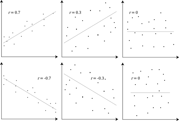
Explain Spearman’s Correlation Coefficient
-
Wikipedia Definition: In statistics, Spearman’s rank correlation coefficient or Spearman’s ρ, named after Charles Spearman is a nonparametric measure of rank correlation (statistical dependence between the rankings of two variables). It assesses how well the relationship between two variables can be described using a monotonic function.
-
Important Inference to keep in mind: The Spearman correlation can evaluate a monotonic relationship between two variables — Continous or Ordinal and it is based on the ranked values for each variable rather than the raw data.
-
What is a monotonic relationship?
- A monotonic relationship is a relationship that does one of the following:
- As the value of one variable increases, so does the value of the other variable, OR,
- As the value of one variable increases, the other variable value decreases.
- But, not exactly at a constant rate whereas in a linear relationship the rate of increase/decrease is constant.
- A monotonic relationship is a relationship that does one of the following:
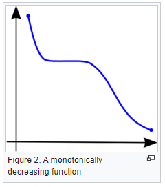
- Example use case: Whether the order in which employees complete a test exercise is related to the number of months they have been employed or correlation between the IQ of a person with the number of hours spent in front of TV per week.
Compare Pearson and Spearman coefficients
- The fundamental difference between the two correlation coefficients is that the Pearson coefficient works with a linear relationship between the two variables whereas the Spearman Coefficient works with monotonic relationships as well.
- One more difference is that Pearson works with raw data values of the variables whereas Spearman works with rank-ordered variables.
- Now, if we feel that a scatterplot is visually indicating a “might be monotonic, might be linear” relationship, our best bet would be to apply Spearman and not Pearson. No harm would be done by switching to Spearman even if the data turned out to be perfectly linear. But, if it’s not exactly linear and we use Pearson’s coefficient then we’ll miss out on the information that Spearman could capture.
-
Let’s look at some examples (source: A comparison of the Pearson and Spearman correlation methods):
- Pearson = +1, Spearman = +1:
- Pearson = +0.851, Spearman = +1 (This is a monotonically increasing relationship, thus Spearman is exactly 1)
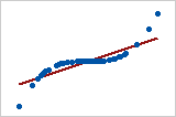
- Pearson = −0.093, Spearman = −0.093
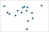
- Pearson = −1, Spearman = −1
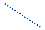
- Pearson = −0.799, Spearman = −1 (This is a monotonically decreasing relationship, thus Spearman is exactly 1)
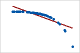
- Note that both of these coefficients cannot capture any other kind of non-linear relationships. Thus, if a scatterplot indicates a relationship that cannot be expressed by a linear or monotonic function, then both of these coefficients must not be used to determine the strength of the relationship between the variables.
How to choose between Pearson and Spearman correlation?
-
If you want to explore your data it is best to compute both, since the relation between the Spearman (S) and Pearson (P) correlations will give some information. Briefly, \(S\) is computed on ranks and so depicts monotonic relationships while \(P\) is on true values and depicts linear relationships.
-
As an example, if you set:
x=(1:100);
y=exp(x);                         % then,
corr(x,y,'type','Spearman');      % will equal 1, and
corr(x,y,'type','Pearson');       % will be about equal to 0.25
- This is because \(y\) increases monotonically with \(x\) so the Spearman correlation is perfect, but not linearly, so the Pearson correlation is imperfect.
corr(x,log(y),'type','Pearson'); % will equal 1
- Doing both is interesting because if you have \(S > P\), that means that you have a correlation that is monotonic but not linear. Since it is good to have linearity in statistics (it is easier) you can try to apply a transformation on \(y\) (such a log).
Explain the central limit theorem and give examples of when you can use it in a real-world problem?
- The center limit theorem states that if any random variable, regardless of the distribution, is sampled a large enough times, the sample mean will be approximately normally distributed. This allows for studying the properties of any statistical distribution as long as there is a large enough sample size.
Describe the motivation behind random forests and mention two reasons why they are better than individual decision trees?
- The motivation behind random forest or ensemble models in general in layman’s terms, Let’s say we have a question/problem to solve we bring 100 people and ask each of them the question/problem and record their solution. Next, we prepare a solution which is a combination/ a mixture of all the solutions provided by these 100 people. We will find that the aggregated solution will be close to the actual solution. This is known as the “Wisdom of the crowd” and this is the motivation behind Random Forests. We take weak learners (ML models) specifically, Decision Trees in the case of Random Forest & aggregate their results to get good predictions by removing dependency on a particular set of features. In regression, we take the mean and for Classification, we take the majority vote of the classifiers.
- A random forest is generally better than a decision tree, however, you should note that no algorithm is better than the other it will always depend on the use case & the dataset [Check the No Free Lunch Theorem in the first comment]. Reasons why random forests allow for stronger prediction than individual decision trees: 1) Decision trees are prone to overfit whereas random forest generalizes better on unseen data as it is using randomness in feature selection as well as during sampling of the data. Therefore, random forests have lower variance compared to that of the decision tree without substantially increasing the error due to bias. 2) Generally, ensemble models like Random Forest perform better as they are aggregations of various models (Decision Trees in the case of Random Forest), using the concept of the “Wisdom of the crowd.”
Mention three ways to make your model robust to outliers?
-
Investigating the outliers is always the first step in understanding how to treat them. After you understand the nature of why the outliers occurred you can apply one of the several methods mentioned below.
-
Add regularization that will reduce variance, for example, L1 or L2 regularization.
-
Use tree-based models (random forest, gradient boosting ) that are generally less affected by outliers.
-
Winsorize the data. Winsorizing or winsorization is the transformation of statistics by limiting extreme values in the statistical data to reduce the effect of possibly spurious outliers. In numerical data, if the distribution is almost normal using the Z-score we can detect the outliers and treat them by either removing or capping them with some value. If the distribution is skewed using IQR we can detect and treat it by again either removing or capping it with some value. In categorical data check for value_count in the percentage if we have very few records from some category, either we can remove it or can cap it with some categorical value like others.
-
Transform the data, for example, you do a log transformation when the response variable follows an exponential distribution or is right-skewed.
-
Use more robust error metrics such as MAE or Huber loss instead of MSE.
-
Remove the outliers, only do this if you are certain that the outliers are true anomalies that are not worth adding to your model. This should be your last consideration since dropping them means losing information.
Given two arrays, write a python function to return the intersection of the two. For example, X = [1,5,9,0] and Y = [3,0,2,9] it should return [9,0]
- A1 (The most repeated one):
set(X).intersect(set(Y))
- A2:
set(X) & set(Y)
-
Using sets is a very good way to do it since it utilizes a hash map implementation underneath it.
-
A3:
def common_func(X, Y):
Z=[]
for i in X:
for j in Y:
if i==j and i not in Z:
Z.append(i)
return Z
- This is also a simple way to do it, however, it leads to the time complexity of O(N*M) so it is better to use sets.
- Some other answers were mentioned that will work for the mentioned case but will return duplicates for other cases, for example, if X = [1,0,9,9] and Y = [3,0,9,9] it will return [0, 9, 9] not [0,9].
A1:
Res=[i for i in x if i in Y]
A2:
Z = [value for value in X if value in Y]
print(Z)
A3:
d = {}
for value in y:
if value not in d:
d[value] = 1
intersection = []
for value in x:
if value in d:
intersection.append(value)

print(intersection)
- The time complexity for this is O(n + m) and the space complexity is O(m), the problem of it is that it returns duplicates.
Given an array, find all the duplicates in this array for example: input: [1,2,3,1,3,6,5] output: [1,3]
- Approach 1:
set1=set()
res=[]
for i in list:
if i in set1:
res.append(i)
else:
set1.add(i)
print(res)
- Approach 2:
arr1=np.array([1,2,3,1,3,6,5])
nums,index,counts=np.unique(arr1,return_index=True,return_counts=True)
print(nums,index,counts)
nums[counts!=1]
- Approach 3:
a=[1,2,3,1,3,6,5]
j=[i for (i,v) in Counter(a).items() if v>1]
Approach 4: Use map (dict), and get the frequency count of each element. Iterate the map, and print all keys whose values are > 1.
What are the differences and similarities between gradient boosting and random forest? and what are the advantage and disadvantages of each when compared to each other?
- Similarities:
- Both these algorithms are decision-tree based algorithms
- Both these algorithms are ensemble algorithms
- Both are flexible models and do not need much data preprocessing.
- Differences:
- Random forests (Uses Bagging): Trees are arranged in a parallel fashion where the results of all trees are aggregated at the end through averaging or majority vote. Gradient boosting (Uses Boosting): Trees are arranged in a series sequential fashion where every tree tries to minimize the error of the previous tree.
- Radnom forests: Every tree is constructed independently of the other trees. Gradient boosting: Every tree is dependent on the previous tree.
- Advantages of gradient boosting over random forests:
- Gradient boosting can be more accurate than Random forests because we train them to minimize the previous tree’s error.
- Gradient boosting is capable of capturing complex patterns in the data.
- Gradient boosting is better than random forest when used on unbalanced data sets.
- Advantages of random forests over gradient boosting :
- Random forest isless prone to overfit as compared to gradient boosting.
- Random forest has faster training as trees are created parallelly & independent of each other.
- The disadvantage of GB over RF:
- Gradient boosting is more prone to overfitting than random forests due to their focus on mistakes during training iterations and the lack of independence in tree building.
- If the data is noisy the boosted trees might overfit and start modeling the noise.
- In GB training might take longer because every tree is created sequentially.
- Tunning the hyperparameters of gradient boosting is harder than those of random forest.
Small file and big file problem in Big data
- The “small file problem” is kind of notorious in the big data space.
- Did you know there’s also the “Big/large file problem”?
- Say you have a billion records. The small file problem would be like.. 10 records per file and 100 million files. Combining all these files is slow, terrible, and has made many data engineers cry.
- The large file problem would be the opposite problem. 1 billion records in 1 file. This is also a huge problem because how do you parallelize 1 file? You can’t without splitting it up first.
- To avoid crying, the solution is sizing your files the right way. Aiming for between 100-200 MBs for file is usually best. In this contrived example, you’d have a 1000 files each with 1 million records.
- It is worth seeing the spread of files and the size and understanding what optimal file size works out best.
- Too low and you have the risk of more files, too high and the parallelism isn’t going to be effective.
- It is recommended to understand up parallelism, and block size and seeing how the distribution of your data (in files) is before adding an arbitrary default file size value.
What are L1 and L2 regularization? What are the differences between the two?
- Regularization is a technique used to avoid overfitting by trying to make the model more simple. One way to apply regularization is by adding the weights to the loss function. This is done in order to consider minimizing unimportant weights. In L1 regularization we add the sum of the absolute of the weights to the loss function. In L2 regularization we add the sum of the squares of the weights to the loss function.
- So both L1 and L2 regularization are ways to reduce overfitting, but to understand the difference it’s better to know how they are calculated:
- Loss (L2) : Cost function + \(L\) * \(weights^2\)
- Loss (L1) : Cost function + \(L\) * \(\|weights\|\)
- Where \(L\) is the regularization parameter
- L2 regularization penalizes huge parameters preventing any of the single parameters to get too large. But weights never become zeros. It adds parameters square to the loss. Preventing the model from overfitting on any single feature.
- L1 regularization penalizes weights by adding a term to the loss function which is the absolute value of the loss. This leads to it removing small values of the parameters leading in the end to the parameter hitting zero and staying there for the rest of the epochs. Removing this specific variable completely from our calculation. So, It helps in simplifying our model. It is also helpful for feature selection as it shrinks the coefficient to zero which is not significant in the model.
What are the Bias and Variance in a Machine Learning Model and explain the bias-variance trade-off?
-
The goal of any supervised machine learning model is to estimate the mapping function (f) that predicts the target variable (y) given input (x). The prediction error can be broken down into three parts:
-
Bias: The bias is the simplifying assumption made by the model to make the target function easy to learn. Low bias suggests fewer assumptions made about the form of the target function. High bias suggests more assumptions made about the form of the target data. The smaller the bias error the better the model is. If the bias error is high, this means that the model is underfitting the training data.
-
Variance: Variance is the amount that the estimate of the target function will change if different training data was used. The target function is estimated from the training data by a machine learning algorithm, so we should expect the algorithm to have some variance. Ideally, it should not change too much from one training dataset to the next, meaning that the algorithm is good at picking out the hidden underlying mapping between the inputs and the output variables. If the variance error is high this indicates that the model overfits the training data.
-
Irreducible error: It is the error introduced from the chosen framing of the problem and may be caused by factors like unknown variables that influence the mapping of the input variables to the output variable. The irreducible error cannot be reduced regardless of what algorithm is used.
-
-
The goal of any supervised machine learning algorithm is to achieve low bias and low variance. In turn, the algorithm should achieve good prediction performance. The parameterization of machine learning algorithms is often a battle to balance out bias and variance.
- For example, if you want to predict the housing prices given a large set of potential predictors. A model with high bias but low variance, such as linear regression will be easy to implement, but it will oversimplify the problem resulting in high bias and low variance. This high bias and low variance would mean in this context that the predicted house prices are frequently off from the market value, but the value of the variance of these predicted prices is low.
- On the other side, a model with low bias and high variance such as a neural network will lead to predicted house prices closer to the market value, but with predictions varying widely based on the input features.
Feature Scaling
- Feature scaling is a preprocessing step in machine learning that aims to bring all features or variables to a similar scale or range. It is essential because many machine learning algorithms perform better when the features are on a similar scale. Here are some common techniques for feature scaling:
1) Standardization (Z-score normalization): This technique scales the features to have zero mean and unit variance. It transforms the data so that it follows a standard normal distribution. Standardization is useful when the features have different scales and the algorithm assumes a Gaussian distribution.
2) Normalization (Min-Max scaling): This technique scales the features to a specific range, usually between 0 and 1. It preserves the relative relationships between data points. Normalization is suitable when the data does not follow a Gaussian distribution and the algorithm does not make assumptions about the distribution.
3) Logarithmic Transformation: This technique applies a logarithmic function to the data. It is useful when the data is skewed or has a wide range of values. Logarithmic transformation can help in reducing the impact of outliers and making the data more normally distributed.
4) Robust Scaling: This technique scales the features based on their interquartile range (IQR). It is similar to standardization but uses the median and IQR instead of the mean and standard deviation. Robust scaling is more resistant to outliers compared to standardization.
When working with AWS, you can use the following toolings for feature scaling:
-
Amazon SageMaker Data Wrangler: It provides built-in transformations for feature scaling, including standardization and normalization. You can preprocess your data using Data Wrangler’s visual interface or through its Python SDK.
-
AWS Glue: It is a fully managed extract, transform, and load (ETL) service. Glue allows you to create and execute data transformation jobs using Apache Spark. You can leverage Spark’s capabilities to perform feature scaling along with other preprocessing steps.
-
Amazon Athena: Athena is an interactive query service that allows you to query data directly from your data lake. You can use SQL queries to perform feature scaling operations within your queries, applying functions like standardization or normalization.
-
These tools provide efficient ways to preprocess and scale your features, enabling you to prepare your data for machine learning tasks effectively.
Briefly explain the A/B testing and its application? What are some common pitfalls encountered in A/B testing?
- A/B testing helps us to determine whether a change in something will cause a change in performance significantly or not. So in other words you aim to statistically estimate the impact of a given change within your digital product (for example). You measure success and counter metrics on at least 1 treatment vs 1 control group (there can be more than 1 XP group for multivariate tests).
- You should rely on experimentation to guide product development not only because it validates or invalidates your hypotheses, but, more important, because it helps create a mentality around building a minimum viable product (MVP) and exploring the terrain around it.
- With experimentation, when you make a strategic bet to bring about a drastic, abrupt change, you test to map out where you’ll land.
- So even if the abrupt change takes you to a lower point initially, you can be confident that you can hill climb from there and reach a greater height
- Used Split.io for NuAIg
- We have guardrail metrics as well to make sure the new release is not causing friction:
- Total revenue per user
- Opt out selected
- Percentage of unique users
- check every KPI and metric important to business
- Applications:
-
Consider the example of a general store that sells bread packets but not butter, for a year. If we want to check whether its sale depends on the butter or not, then suppose the store also sells butter and sales for next year are observed. Now we can determine whether selling butter can significantly increase/decrease or doesn’t affect the sale of bread.
-
While developing the landing page of a website you create 2 different versions of the page. You define a criteria for success eg. conversion rate. Then define your hypothesis,
- Null hypothesis (H): No difference between the performance of the 2 versions.
- Alternative hypothesis (H’): version A will perform better than B.
-
-
Note that you will have to split your traffic randomly (to avoid sample bias) into 2 versions. The split doesn’t have to be symmetric, you just need to set the minimum sample size for each version to avoid undersample bias.
-
Now if version A gives better results than version B, we will still have to statistically prove that results derived from our sample represent the entire population. Now one of the very common tests used to do so is 2 sample t-test where we use values of significance level (alpha) and p-value to see which hypothesis is right. If p-value<alpha, H is rejected.
- Common pitfalls:
- Wrong success metrics inadequate to the business problem
- Lack of counter metric, as you might add friction to the product regardless along with the positive impact
- Sample mismatch: heterogeneous control and treatment, unequal variances
- Underpowered test: too small sample or XP running too short 5. Not accounting for network effects (introduce bias within measurement)
Best practices for A/B Testing
- Taken from here
- Measure one change at a time.
- This is not to say that you can only test one thing at a time, but that you have to design your experiment properly so that you are able to measure one change at a time. At LinkedIn, a product launch usually involves multiple features/components. One big upgrade to LinkedIn Search in 2013 introduced unified search across different product categories. With this functionality, the search box is smart enough to figure out query intent without explicit input on categories such as “People,” or “Jobs,” or “Companies.”
- However, that was not all. Almost every single component on the search landing-page was touched, from the left rail navigation to snippets and action buttons. The first experiment was run with all changes lumped together. To our surprise, many key metrics tanked. It was a lengthy process to bring back one feature at a time in order to figure out the true culprit. In the end, we realized that several small changes, not the unified search itself, were responsible for bringing down clicks and revenue. After restoring these features, unified search was shown to be positive to user experience and deployed to everyone.
- Decide on triggered users, but report on all users.
- It is very common that an experiment only impacts a small fraction of your user base. For example, we want to automatically help people fill in their patents on their LinkedIn profiles, but not every member has a patent. So the experiment would only be affecting those ~5% of members who have filed patents. To measure how much benefit this is bringing to our members, we have to focus on this small subsegment, the “triggered” users. Otherwise, the signal from that 5% of users would be lost in the 95% noise. However, once we determined that patents are a beneficial feature, we needed to have a “realistic” estimate of the overall impact. How is LinkedIn’s bottom line going to change once this feature is rolled out universally? Having such a “site-wide” impact not only makes it possible to compare impacts across experiments, but also easy to quantify ROI.
- The experimental group should not be influenced by the experiment outcomes.
- The fundamental assumption of A/B testing is that the difference between the A and B groups is only caused by the treatment we impose. It may be obvious that we need to make sure the users in A and B are similar enough to begin with. The standard approach to check for any pre-existing differences is to run an A/A test before the actual A/B test, where both groups of users receive identical treatments. However, it is equally important to make sure the user groups stay “similar” during the experiment especially in the online world because the experimental population is usually “dynamic”. As an example, we tested a new feature where members received a small banner on their LinkedIn profile page to encourage them to explore our new homepage. Only users who had not visited the homepage recently were eligible to be in the experiment, and the eligibility was dynamically updated after a user visited the homepage. Because the banner brought more users in the treatment group to visit the homepage, more treatment users became ineligible over time. Because these “additionally” removed users tend to be more active than the rest, we artificially created a difference between users in A and B as the test continued. In general, if the experimental population is directly influenced by the experiment outcomes, we are likely to see a bias. Such bias could void the experiment results because it usually overwhelms any real signal resulting from the treatment itself.
- Avoid coupling a marketing campaign with an A/B test.
- We have recently revamped the Who Viewed My Profile page. The product team wanted to measure through an A/B test if the changes are indeed better, and if so, by how much. The marketing team wanted to create buzz around the new page with an email campaign. This is a very common scenario, but how can the A/B test and the email campaign coexist? Clearly, we can only send campaign emails to the treatment group, since there is nothing new for members in control. However, such a campaign would contaminate the online A/B test because it encourages more members from the treatment to visit. These additional users tend to be less engaged, therefore we are likely to see an artificial drop in key metrics. It is best to measure the A/B test first before launching the campaign.
- Use a simple rule of thumb to address multiple testing problems.
- Multiple testing problems are extremely prevalent in online A/B testing. The symptom is that irrelevant metrics appear to be statistically significant. The root cause is usually because too many metrics are examined simultaneously (keep in mind that we compute over 1000 metrics for each experiment). Even though we have tried to educate people on the topic of multiple testing, many are still clueless about what they should do when a metric is unexpectedly significant. Should they trust it or treat it as noise? Instead, we have found it very effective to introduce a simple rule of thumb: Use the standard 0.05 p-value cutoff for metrics that are expected to be impacted, but use a smaller cutoff, say 0.001, for metrics that are not. The rule-of-thumb is based on an interesting Bayesian interpretation. It boils down to how much we believe a metric will be impacted before we even run the experiment. In particular, if using 0.05 reflects a prior probability of 50%, then using 0.001 means a much weaker belief - at about 2%.
- These are only a few best practices for experimentation, but they’ve proven crucial for product development at LinkedIn. As I’ve said before, A/B testing and making data driven decisions through experimentation is an extremely important part of the culture at LinkedIn. It guides how and why we build products for our users by giving us crucial data on how they actually use our services. By following these five lessons, developers across all companies and industries can not only make more informed decisions about their products, but also create a better experience for the people using them.
Mention three ways to handle missing or corrupted data in adataset?
-
In general, real-world data often has a lot of missing values. The cause of missing values can be data corruption or failure to record data. The handling of missing data is very important during the preprocessing of the dataset as many machine learning algorithms do not support missing values. However, you should start by asking the data owner/stakeholder about the missing or corrupted data. It might be at the data entry level, because of file encoding, etc. which if aligned, can be handled without the need to use advanced techniques.
-
There are different ways to handle missing data, we will discuss only three of them:
-
Deleting the row with missing values
- The first method to handle missing values is to delete the rows or columns that have null values. This is an easy and fast method and leads to a robust model, however, it will lead to the loss of a lot of information depending on the amount of missing data and can only be applied if the missing data represent a small percentage of the whole dataset.
-
Using learning algorithms that support missing values
- Some machine learning algorithms are robust to missing values in the dataset. The K-NN algorithm can ignore a column from a distance measure when there are missing values. Naive Bayes can also support missing values when making a prediction. Another algorithm that can handle a dataset with missing values or null values is the random forest model and Xgboost (check the post in the first comment), as it can work on non-linear and categorical data. The problem with this method is that these models’ implementation in the scikit-learn library does not support handling missing values, so you will have to implement it yourself.
-
Missing value imputation
- Data imputation means the substitution of estimated values for missing or inconsistent data in your dataset. There are different ways to estimate the values that will replace the missing value. The simplest one is to replace the missing value with the most repeated value in the row or the column. Another simple way is to replace it with the mean, median, or mode of the rest of the row or the column. This advantage of this is that it is an easy and fast way to handle the missing data, but it might lead to data leakage and does not factor the covariance between features. A better way is to use a machine learning model to learn the pattern between the data and predict the missing values, this is a very good method to estimate the missing values that will not lead to data leakage and will factor the covariance between the feature, the drawback of this method is the computational complexity especially if your dataset is large.
-
How do you avoid #overfitting? Try one (or more) of the following:
-
Training with more data, which makes the signal stronger and clearer, and can enable the model to detect the signal better. One way to do this is to use #dataaugmentation strategies
-
Reducing the number of features in order to avoid the curse of dimensionality (which occurs when the amount of data is too low to support highly-dimensional models), which is a common cause for overfitting
-
Using cross-validation. This technique works because the model is unlikely to make the same mistake on multiple different samples, and hence, errors will be evened out
-
Using early stopping to end the training process before the model starts learning the noise
-
Using regularization and minimizing the adjusted loss function. Regularization works because it discourages learning a model that’s overly complex or flexible
-
Using ensemble learning, which ensures that the weaknesses of a model are compensated by the other ones
Data science /#MLinterview are hard - regardless which side of the table you are on.
-
As a jobseeker, it can be really hard to shine, especially when the questions asked have little to no relevance to the actual job. How are you supposed to showcase your ability to build models when the entire interview revolves are binary search trees?
-
As a hiring manager, it’s close to impossible to evaluate modeling skills by just talking to someone, and false positives are really frequent. A question that dramatically reduces the noise on both sides:
“What is the most machine learning complex concept you came across, and how would you explain it to yourself that would have made it easier for you to understand it before you learned it?”
-
The answer will tell you a lot more about the candidate than you might think:
- 90% of candidates answer “overfitting”. If they’re junior and explain it really well and they’re junior, it means they’re detailed-oriented and try to gain a thorough understanding of the field, but they sure could show more ambition; if they don’t, it means their understanding of the fundamentals is extremely basic.
- If they answer back-propagation, and they can explain it well, it means they’re more math-oriented than the average and will probably be a good candidate for a research role as an applied DS role.
- If their answer has something to do with a brand-new ML concept, , and they can explain it well, it means they’re growth-oriented and well-read.
- Generally speaking, if they answer something overly complicated and pompous, but can’t explain it well, it means they’re trying to impress but have an overall shallow understanding - a good rule of thumb is not hire them.
- Now, if you are a candidate, or an ML professional, keep asking yourself that question: “What is the most sophisticated concept, model or architecture you know of?” If you keep giving the same answer, maybe you’ve become complacent, and it’s time for you to learn something new.
- How would you explain it to a newbie? As Einstein said, if “you can’t explain it simply, you don’t understand it well enough”.
Order of execution of an SQL Query in Detail
-
Each query begins with finding the data that we need in a database, and then filtering that data down into something that can be processed and understood as quickly as possible.
-
Because each part of the query is executed sequentially, it’s important to understand the order of execution so that you know what results are accessible where.
-
Consider the below mentioned query :
SELECT DISTINCT column, AGG_FUNC(column_or_expression), …
FROM mytable
JOIN another_table
ON mytable.column = another_table.column
WHERE constraint_expression
GROUP BY column
HAVING constraint_expression
ORDER BY column ASC/DESC
LIMIT count OFFSET COUNT;
- Query order of execution:
1.FROMandJOINs
- TheFROMclause, and subsequentJOINs are first executed to determine the total working set of data that is being queried. This includes subqueries in this clause, and can cause temporary tables to be created under the hood containing all the columns and rows of the tables being joined.
2.WHERE
- Once we have the total working set of data, the first-passWHEREconstraints are applied to the individual rows, and rows that do not satisfy the constraint are discarded. Each of the constraints can only access columns directly from the tables requested in theFROMclause. Aliases in theSELECTpart of the query are not accessible in most databases since they may include expressions dependent on parts of the query that have not yet executed.
3.GROUP BY
- The remaining rows after theWHEREconstraints are applied are then grouped based on common values in the column specified in theGROUP BYclause. As a result of the grouping, there will only be as many rows as there are unique values in that column. Implicitly, this means that you should only need to use this when you have aggregate functions in your query.
4.HAVING
- If the query has aGROUP BYclause, then the constraints in theHAVINGclause are then applied to the grouped rows, discard the grouped rows that don’t satisfy the constraint. Like theWHEREclause, aliases are also not accessible from this step in most databases.
5.SELECT
- Any expressions in theSELECTpart of the query are finally computed.
6.DISTINCT
- Of the remaining rows, rows with duplicate values in the column marked asDISTINCTwill be discarded.
7.ORDER BY
- If an order is specified by theORDER BYclause, the rows are then sorted by the specified data in either ascending or descending order. Since all the expressions in theSELECTpart of the query have been computed, you can reference aliases in this clause.
8.LIMIT/OFFSET
- Finally, the rows that fall outside the range specified by theLIMITandOFFSETare discarded, leaving the final set of rows to be returned from the query.
Explain briefly the logistic regression model and state an example of when you have used it recently?
- Logistic regression is used to calculate the probability of occurrence of an event in the form of a dependent output variable based on independent input variables. Logistic regression is commonly used to estimate the probability that an instance belongs to a particular class. If the probability is bigger than 0.5 then it will belong to that class (positive) and if it is below 0.5 it will belong to the other class. This will make it a binary classifier.
- It is important to remember that the Logistic regression isn’t a classification model, it’s an ordinary type of regression algorithm, and it was developed and used before machine learning, but it can be used in classification when we put a threshold to determine specific categories.
- There is a lot of classification applications to it: classify email as spam or not, identify whether the patient is healthy or not, etc.
Describe briefly the hypothesis testing and p-value in layman’s terms? And give a practical application for them?
- In Layman’s terms:
- Hypothesis test is where you have a current state (null hypothesis) and an alternative state (alternative hypothesis). You assess the results of both of the states and see some differences. You want to decide whether the difference is due to the alternative approach or not.
- You use the p-value to decide this, where the p-value is the likelihood of getting the same results the alternative approach achieved if you keep using the existing approach. It’s the probability to find the result in the gaussian distribution of the results you may get from the existing approach.
- The rule of thumb is to reject the null hypothesis if the p-value < 0.05, which means that the probability to get these results from the existing approach is <95%. But this % changes according to task and domain.
- To explain the hypothesis testing in layman’s term with an example, suppose we have two drugs A and B, and we want to determine whether these two drugs are the same or different. This idea of trying to determine whether the drugs are the same or different is called hypothesis testing. The null hypothesis is that the drugs are the same, and the p-value helps us decide whether we should reject the null hypothesis or not.
- p-values are numbers between 0 and 1, and in this particular case, it helps us to quantify how confident we should be to conclude that drug A is different from drug B. The closer the p-value is to 0, the more confident we are that the drugs A and B are different.
What is an activation function and discuss the use of an activation function? Explain three different types of activation functions?
- In mathematical terms, the activation function serves as a gate between the current neuron input and its output, going to the next level. Basically, it decides whether neurons should be activated or not. It is used to introduce non-linearity into a model.
- Activation functions are added to introduce non-linearity to the network, it doesn’t matter how many layers or how many neurons your net has, the output will be linear combinations of the input in the absence of activation functions. In other words, activation functions are what make a linear regression model different from a neural network. We need non-linearity, to capture more complex features and model more complex variations that simple linear models can not capture.
- There are a lot of activation functions:
- Sigmoid function: \(f(x) = 1/(1+exp(-x))\).
- The output value of it is between 0 and 1, we can use it for classification. It has some problems like the gradient vanishing on the extremes, also it is computationally expensive since it uses exp.
- ReLU: \(f(x) = max(0,x)\).
- it returns 0 if the input is negative and the value of the input if the input is positive. It solves the problem of vanishing gradient for the positive side, however, the problem is still on the negative side. It is fast because we use a linear function in it.
- Leaky ReLU:
- Sigmoid function: \(f(x) = 1/(1+exp(-x))\).
- It solves the problem of vanishing gradient on both sides by returning a value “a” on the negative side and it does the same thing as ReLU for the positive side.
- Softmax: it is usually used at the last layer for a classification problem because it returns a set of probabilities, where the sum of them is 1. Moreover, it is compatible with cross-entropy loss, which is usually the loss function for classification problems.
If you roll a dice three times, what is the probability to get two consecutive threes?
- The answer is 11/216.
- There are different ways to answer this question:
- If we roll a dice three times we can get two consecutive 3’s in three ways:
- The first two rolls are 3s and the third is any other number with a probability of 1/6 * 1/6 * 5/6.
- The first one is not three while the other two rolls are 3s with a probability of 5/6 * 1/6 * 1/6.
- The last one is that the three rolls are 3s with probability 1/6 ^ 3.
- So the final result is \(2 * (5/6 * (1/6)^2) + (1/6)*3 = 11/216\).
- By Inclusion-Exclusion Principle:
- Probability of at least two consecutive threes: = Probability of two consecutive threes in first two rolls + Probability of two consecutive threes in last two rolls - Probability of three consecutive threes = 2Probability of two consecutive threes in first two rolls - Probability of three consecutive threes = 21/61/6 - 1/61/6*1/6 = 11/216
- It can be seen also like this:
- The sample space is made of (x, y, z) tuples where each letter can take a value from 1 to 6, therefore the sample space has 6x6x6=216 values, and the number of outcomes that are considered two consecutive threes is (3,3, X) or (X, 3, 3), the number of possible outcomes is therefore 6 for the first scenario (3,3,1) till (3,3,6) and 6 for the other scenario (1,3,3) till (6,3,3) and subtract the duplicate (3,3,3) which appears in both, and this leaves us with a probability of 11/216.
- If we roll a dice three times we can get two consecutive 3’s in three ways:
You and your friend are playing a game with a fair coin. The two of you will continue to toss the coin until the sequence HH or TH shows up. If HH shows up first, you win, and if TH shows up first your friend win. What is the probability of you winning the game?
- If T is ever flipped, you cannot then reach HH before your friend reaches TH. Therefore, the probability of you winning this is to flip HH initially. Therefore the sample space will be {HH, HT, TH, TT} and the probability of you winning will be (1/4) and your friend (3/4).
Dimensionality reduction techniques
-
Dimensionality reduction techniques help deal with the curse of dimensionality. Some of these are supervised learning approaches whereas others are unsupervised. Here is a quick summary:
- PCA - Principal Component Analysis is an unsupervised learning approach and can Handle skewed data easily for dimensionality reduction.
- LDA - Linear Discriminant Analysis is also a dimensionality reduction technique based on eigenvectors but it also maximizes class separation while doing so. Moreover, it is a supervised Learning approach and it performs better with uniformly distributed data.
- ICA - Independent Component Analysis aims to maximize the statistical independence between variables and is a Supervised learning approach.
- MDS - Multi dimensional scaling aims to preserve the Euclidean pairwise distances. It is an Unsupervised learning approach.
- ISOMAP - Also known as Isometric Mapping is another dimensionality reduction technique which preserves geodesic pairwise distances. It is an unsupervised learning approach. It can handle noisy data well.
- t-SNE - Called the t-distributed stochastic neighbor embedding preserves local structure and is an Unsupervised learning approach.
Active learning
- Active learning is a semi-supervised ML training paradigm which, like all semi-supervised learning techniques, relies on the usage of partially labeled data.
- Active Learning consists of dynamically selecting the most relevant data by sequentially:
- selecting a sample of the raw (unannotated) dataset (the algorithm used for that selection step is called a querying strategy).
- getting the selected data annotated.
- training the model with that sample of annotated training data.
- running inference on the remaining (unannotated) data.
- That last step is used to evaluate which records should be then selected for the next iteration (called a loop). However, since there is no ground truth for the data used in the inference step, one cannot simply decide to feed the – data where the model failed to make the correct prediction, and has instead to use metadata (such as the confidence level of the prediction) to make that decision.
- The easiest and most common querying strategy used for selecting the next batch of useful data consists of picking the records with the lowest confidence level; this is called the least-confidence querying strategy, which is one of many possible querying strategies.
What is the independence assumption for a Naive Bayes classifier?
- Naive bayes assumes that the feature probabilities are independent given the class \(c\), i.e., the features do not depend on each other are totally uncorrelated.
- This is why the Naive Bayes algorithm is called “naive”.
-
Mathematically, the features are independent given class:
\[\begin{aligned} P\left(X_{1}, X_{2} \mid Y\right) &=P\left(X_{1} \mid X_{2}, Y\right) P\left(X_{2} \mid Y\right) \\ &=P\left(X_{1} \mid Y\right) P\left(X_{2} \mid Y\right) \end{aligned}\]- More generally: \(P\left(X_{1} \ldots X_{n} \mid Y\right)=\prod_{i} P\left(X_{i} \mid Y\right)\)
Explain briefly batch gradient descent, stochastic gradient descent, and mini-batch gradient descent? List the pros and cons of each.
- Gradient descent is a generic optimization algorithm capable for finding optimal solutions to a wide range of problems. The general idea of gradient descent is to tweak parameters iteratively in order to minimize a cost function.
- Batch Gradient Descent:
- In Batch Gradient descent the whole training data is used to minimize the loss function by taking a step towards the nearest minimum by calculating the gradient (the direction of descent).
- Pros:
- Since the whole data set is used to calculate the gradient it will be stable and reach the minimum of the cost function without bouncing around the loss function landscape (if the learning rate is chosen correctly).
- Cons:
- Since batch gradient descent uses all the training set to compute the gradient at every step, it will be very slow especially if the size of the training data is large.
- Stochastic Gradient Descent:
- Stochastic Gradient Descent picks up a random instance in the training data set at every step and computes the gradient-based only on that single instance.
- Pros:
- It makes the training much faster as it only works on one instance at a time.
- It become easier to train using large datasets.
- Cons:
- Due to the stochastic (random) nature of this algorithm, this algorithm is much less stable than the batch gradient descent. Instead of gently decreasing until it reaches the minimum, the cost function will bounce up and down, decreasing only on average. Over time it will end up very close to the minimum, but once it gets there it will continue to bounce around, not settling down there. So once the algorithm stops, the final parameters would likely be good but not optimal. For this reason, it is important to use a training schedule to overcome this randomness.
- Mini-batch Gradient:
- At each step instead of computing the gradients on the whole data set as in the Batch Gradient Descent or using one random instance as in the Stochastic Gradient Descent, this algorithm computes the gradients on small random sets of instances called mini-batches.
- Pros:
- The algorithm’s progress space is less erratic than with Stochastic Gradient Descent, especially with large mini-batches.
- You can get a performance boost from hardware optimization of matrix operations, especially when using GPUs.
- Cons:
- It might be difficult to escape from local minima.
- Batch Gradient Descent:
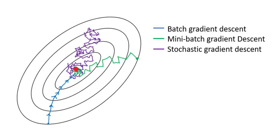
Explain what is information gain and entropy in the context of decision trees?
- Entropy and Information Gain are two key metrics used in determining the relevance of decision making when constructing a decision tree model and to determine the nodes and the best way to split.
- The idea of a decision tree is to divide the data set into smaller data sets based on the descriptive features until we reach a small enough set that contains data points that fall under one label.
- Entropy is the measure of impurity, disorder, or uncertainty in a bunch of examples. Entropy controls how a Decision Tree decides to split the data. Information gain calculates the reduction in entropy or surprise from transforming a dataset in some way. It is commonly used in the construction of decision trees from a training dataset, by evaluating the information gain for each variable, and selecting the variable that maximizes the information gain, which in turn minimizes the entropy and best splits the dataset into groups for effective classification.
What are some applications of RL beyond gaming and self-driving cars?
- Reinforcement learning is NOT just used in gaming and self-driving cars, here are three common use cases you should know in 2022:
-
Multi-arm bandit testing (MAB)
- A little bit about reinforcement learning (RL): you train an agent to interact with the environment and figure out the optimum policy which maximizes the reward (a metric you select).
- MAB is a classic reinforcement learning problem that can be used to help you find a best options out of a lot of treatments in experimentation.
- Unlike A/B tests, MAB tries to maximizes a metric (reward) during the course of the test. It usually has a lot of treatments to select from. The trade-off is that you can draw causal inference through traditional A/B testing, but it’s hard to analyze each treatment through MAB; however, because it’s dynamic, it might be faster to select the best treatment than A/B testing.
-
Recommendation engines
- While traditional matrix factorization works well for recommendation engines, using reinforcement learning can help you maximize metrics like customer engagement and metrics that measure downstream impact.
- For example, social media can use RL to maximize ‘time spent’ or ‘review score’ when recommending content; so this way, instead of just recommending similar content, you might also help customers discover new content or other popular content they like.
-
Portfolio Management
- RL has been used in finance recently as well. Data scientist can train the agent to interact with a trading environment to maximize the return of the portfolio. For example, if the agent selects an allocation of 70% stock, 10% Cash, and 20% bond, the agent gets a positive or negative reward for this allocation. Through iteration, the agent finds out the best allocation.
- Robo-advisers can also use RL to learn investors risk tolerance.
- Of course, self-driving cars, gaming, robotics use RL heavily, but I’ve seen data scientists from industries mentioned above (retail, social media, finance) start to use more RL in their day-to-day work.
You are using a deep neural network for a prediction task. After training your model, you notice that it is strongly overfitting the training set and that the performance on the test isn’t good. What can you do to reduce overfitting?
- To reduce overfitting in a deep neural network changes can be made in three places/stages: The input data to the network, the network architecture, and the training process:
- The input data to the network:
- Check if all the features are available and reliable
- Check if the training sample distribution is the same as the validation and test set distribution. Because if there is a difference in validation set distribution then it is hard for the model to predict as these complex patterns are unknown to the model.
- Check for train / valid data contamination (or leakage)
- The dataset size is enough, if not try data augmentation to increase the data size
- The dataset is balanced
- Network architecture:
- Overfitting could be due to model complexity. Question each component:
- can fully connect layers be replaced with convolutional + pooling layers?
- what is the justification for the number of layers and number of neurons chosen? Given how hard it is to tune these, can a pre-trained model be used?
- Add regularization - ridge (l1), lasso (l2), elastic net (both)
- Add dropouts
- Add batch normalization
- The training process:
- Improvements in validation losses should decide when to stop training. Use callbacks for early stopping when there are no significant changes in the validation loss and restore_best_weights.
Explain the linear regression model and discuss its assumption?
- Linear regression is a supervised statistical model to predict dependent variable quantity based on independent variables.
- Linear regression is a parametric model and the objective of linear regression is that it has to learn coefficients using the training data and predict the target value given only independent values.
- Some of the linear regression assumptions and how to validate them:
- Linear relationship between independent and dependent variables
- Independent residuals and the constant residuals at every \(x\): We can check for 1 and 2 by plotting the residuals(error terms) against the fitted values (upper left graph). Generally, we should look for a lack of patterns and a consistent variance across the horizontal line.
- Normally distributed residuals: We can check for this using a couple of methods: -Q-Q-plot(upper right graph): If data is normally distributed, points should roughly align with the 45-degree line. -Boxplot: it also helps visualize outliers -Shapiro–Wilk test: If the p-value is lower than the chosen threshold, then the null hypothesis (Data is normally distributed) is rejected.
- Low multicollinearity
- You can calculate the VIF (Variable Inflation Factors) using your favorite statistical tool. If the value for each covariate is lower than 10 (some say 5), you’re good to go.
- The figure below summarizes these assumptions.
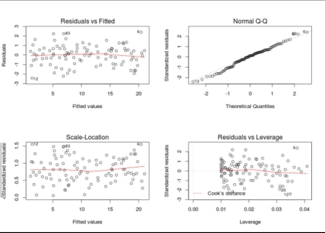
Explain briefly the K-Means clustering and how can we find the best value of K?
- K-Means is a well-known clustering algorithm. K-Means clustering is often used because it is easy to interpret and implement. It starts by partitioning a set of data into \(K\) distinct clusters and then arbitrary selects centroids of each of these clusters. It iteratively updates partitions by first assigning the points to the closet cluster and then updating the centroid and then repeating this process until convergence. The process essentially minimizes the total inter-cluster variation across all clusters.
- The elbow method is a well-known method to find the best value of \(K\) in K-means clustering. The intuition behind this technique is that the first few clusters will explain a lot of the variation in the data, but past a certain point, the amount of information added is diminishing. Looking at the graph below of the explained variation (on the y-axis) versus the number of cluster \(K\) (on the x-axis), there should be a sharp change in the y-axis at some level of \(K\). For example in the graph below the drop-off is at \(k=3\).
- The explained variation is quantified by the within-cluster sum of squared errors. To calculate this error notice, we look for each cluster at the total sum of squared errors using Euclidean distance.
- Another popular alternative method to find the value of \(K\) is to apply the silhouette method, which aims to measure how similar points are in its cluster compared to other clusters. It can be calculated with this equation: \((x-y)/max(x,y)\), where \(x\) is the mean distance to the examples of the nearest cluster, and \(y\) is the mean distance to other examples in the same cluster. The coefficient varies between -1 and 1 for any given point. A value of 1 implies that the point is in the right cluster and the value of -1 implies that it is in the wrong cluster. By plotting the silhouette coefficient on the y-axis versus each \(K\) we can get an idea of the optimal number of clusters. However, it is worthy to note that this method is more computationally expensive than the previous one.
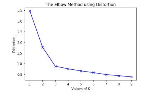
Given an integer array, return the maximum product of any three numbers in the array.
- For example:
A = [1, 5, 3, 4] it should return 60
B = [-2, -4, 5, 3] it should return 40
- If all the numbers are positive, then the solution will be finding the max 3 numbers, if they have negative numbers then it will be the result of multiplying the smallest two negative numbers with the maximum positive number.
- We can use the
heapqlibrary to sort and find the maximum numbers in one step. As shown in the image below.
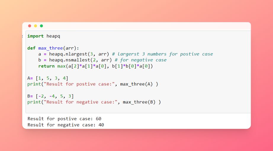
What are joins in SQL and discuss its types?
- A JOIN clause is used to combine rows from two or more tables, based on a related column between them. It is used to merge two tables or retrieve data from there. There are 4 types of joins: inner join left join, right join, and full join.
- Inner join: Inner Join in SQL is the most common type of join. It is used to return all the rows from multiple tables where the join condition is satisfied.
- Left Join: Left Join in SQL is used to return all the rows from the left table but only the matching rows from the right table where the join condition is fulfilled.
- Right Join: Right Join in SQL is used to return all the rows from the right table but only the matching rows from the left table where the join condition is fulfilled.
- Full Join: Full join returns all the records when there is a match in any of the tables. Therefore, it returns all the rows from the left-hand side table and all the rows from the right-hand side table.
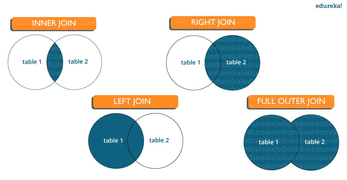
Why should we use Batch Normalization?
- Batch normalization is a technique for training very deep neural networks that standardizes the inputs to a layer for each mini-batch.
- Usually, a dataset is fed into the network in the form of batches where the distribution of the data differs for every batch size. By doing this, there might be chances of vanishing gradient or exploding gradient when it tries to backpropagate. In order to combat these issues, we can use BN (with irreducible error) layer mostly on the inputs to the layer before the activation function in the previous layer and after fully connected layers.
- Batch Normalisation has the following effects on the Neural Network:
- Robust Training of the deeper layers of the network.
- Better covariate-shift proof NN Architecture.
- Has a slight regularization effect.
- Centered and controlled values of Activation.
- Tries to prevent exploding/vanishing gradient.
- Faster training/convergence.
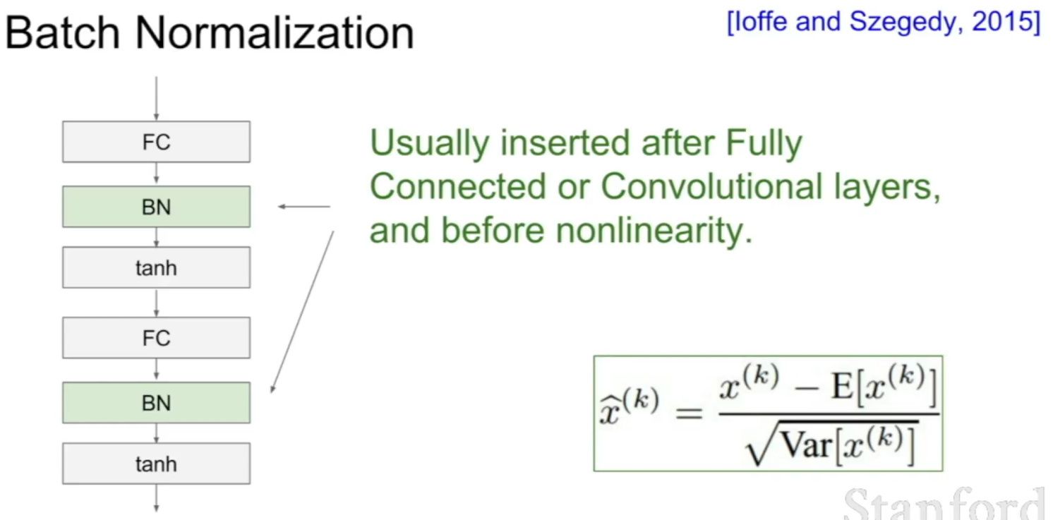
What is weak supervision?
- Weak Supervision (which most people know as the Snorkel algorithm) is an approach designed to help annotate data at scale, and it’s a pretty clever one too.
- Imagine that you have to build a content moderation system that can flag LinkedIn posts that are offensive. Before you can build a model, you’ll first have to get some data. So you’ll scrape posts. A lot of them, because content moderation is particularly data-greedy. Say, you collect 10M of them. That’s when trouble begins: you need to annotate each and every one of them - and you know that’s gonna cost you a lot of time and a lot of money!
- So you want to use autolabeling (basically, you want to apply a pre-trained model) to generate ground truth. The problem is that such a model doesn’t just lie around, as this isn’t your vanilla object detection for autonomous driving use case, and you can’t just use YOLO v5.
- Rather than seek the budget to annotate all that data, you reach out to subject matter experts you know on LinkedIn, and you ask them to give you a list of rules of what constitutes, according to each one of them, an offensive post.
Person 1's rules:
- The post is in all caps
- There is a mention of Politics

Person 2's rules:
- The post is in all caps
- It uses slang
- The topic is not professional

...

Person 20's rules:
- The post is about religion
- The post mentions death
- You then combine all rules into a mega processing engine that functions as a voting system: if a comment is flagged as offensive by at least X% of those 20 rule sets, then you label it as offensive. You apply the same logic to all 10M records and are able to annotate then in minutes, at almost no costs.
- You just used a weakly supervised algorithm to annotate your data.
- You can of course replace people’s inputs by embeddings, or some other automatically generated information, which comes handy in cases when no clear rules can be defined (for example, try coming up with rules to flag a cat in a picture).
What is active learning?
- When you don’t have enough labeled data and it’s expensive and/or time consuming to label new data, active learning is the solution. Active learning is a semi-supervised ML training paradigm which, like all semi-supervised learning techniques, relies on the usage of partially labeled data. Active Learning helps to select unlabeled samples to label that will be most beneficial for the model, when retrained with the new sample.
- Active Learning consists of dynamically selecting the most relevant data by sequentially:
- selecting a sample of the raw (unannotated) dataset (the algorithm used for that selection step is called a querying strategy)
- getting the selected data annotated
- training the model with that sample of annotated training data
- running inference on the remaining (unannotated) data.
- That last step is used to evaluate which records should be then selected for the next iteration (called a loop). However, since there is no ground truth for the data used in the inference step, one cannot simply decide to feed the data where the model failed to make the correct prediction, and has instead to use metadata (such as the confidence level of the prediction) to make that decision.
- The easiest and most common querying strategy used for selecting the next batch of useful data consists of picking the records with the lowest confidence level; this is called the least-confidence querying strategy, which is one of many possible querying strategies. (Technically, those querying strategies are usually brute-force, arbitrary algorithms which can be replaced by actual ML models trained on metadata generated during the training and inference phases for more sophistication).
- Thus, the most important criterion is selecting samples with maximum prediction uncertainty. You can use the model’s prediction confidence to ascertain uncertain samples. Entropy is another way to measure such uncertainty. Another criterion could be diversity of the new sample with respect to exiting training data. You could also select samples close to labeled samples in the training data with poor performance. Another option could be selecting samples from regions of the feature space where better performance is desired. You could combine all the strategies in your active learning decision making process.
- The training is an iterative process. With active learning you select new sample to label, label it and retrain the model. Adding one labeled sample at a time and retraining the model could be expensive. There are techniques to select a batch of samples to label. For deep learning the most popular active learning technique is entropy with is Monte Carlo dropout for prediction probability.
- The process of deciding the samples to label could also be implemented with Multi Arm Bandit. The reward function could be defined in terms of prediction uncertainty, diversity, etc.
- Let’s go deeper and explain why the vanilla form of Active Learning, “uncertainty-based”/”least-confidence” Active Learning, actually perform poorly via real-life datasets:
- Let’s take the example of a binary classification model identifying toxic content in tweets, and let’s say we have 100,000 tweets as our dataset.
- Here is how uncertainty-based AL would work:
- We pick 1,000 (or another number, depending on how we tune the process) records - at that stage, randomly.
- We annotate that data as toxic / not-toxic.
- We train our model with it and get a (not-so-good) model.
- We use the model to infer the remaining 99,000 (unlabeled) records.
- We don’t have ground truth for those 99,000, so we can’t select which records are incorrectly predicted, but we can use metadata, such as the confidence level, as a proxy to detect bad predictions. With least confidence Active Learning, we would pick the 1,000 records predicted with the lowest confidence level as our next batch.
- Go to (2) and repeat the same steps, until we’re happy with the model.
- What we did here, is assume that confidence was a good proxy for usefulness, because it is assumed that low confidence records are the hardest for the model to learn, and hence that the model needs to see them to learn more efficiently.
- Let’s consider a scenario where it is not. Assume now that this training data is not clean, and 5% of the data is actually in Spanish. If the model (and the majority of the data) was meant to be for English, then chances are, the Spanish tweets will be inferred with a low confidence: you will actually pollute the dataset with data that doesn’t belong there. In other words, low confidence can happen for a variety of different reasons. That’s what happens when you do active learning with messy data.
- To resolve this, one solution is to stop using confidence level alone: confidence levels are just one meta-feature to evaluate usefulness.
- In a nutshell, active learning is an incremental semi-supervised learning paradigm where training data is selected incrementally and the model is sequentially retrained (loop after loop), until either the model reaches a specific performance or labeling budget is exhausted.
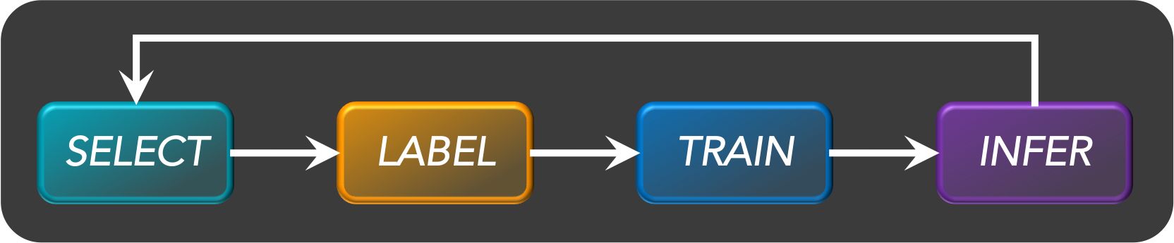
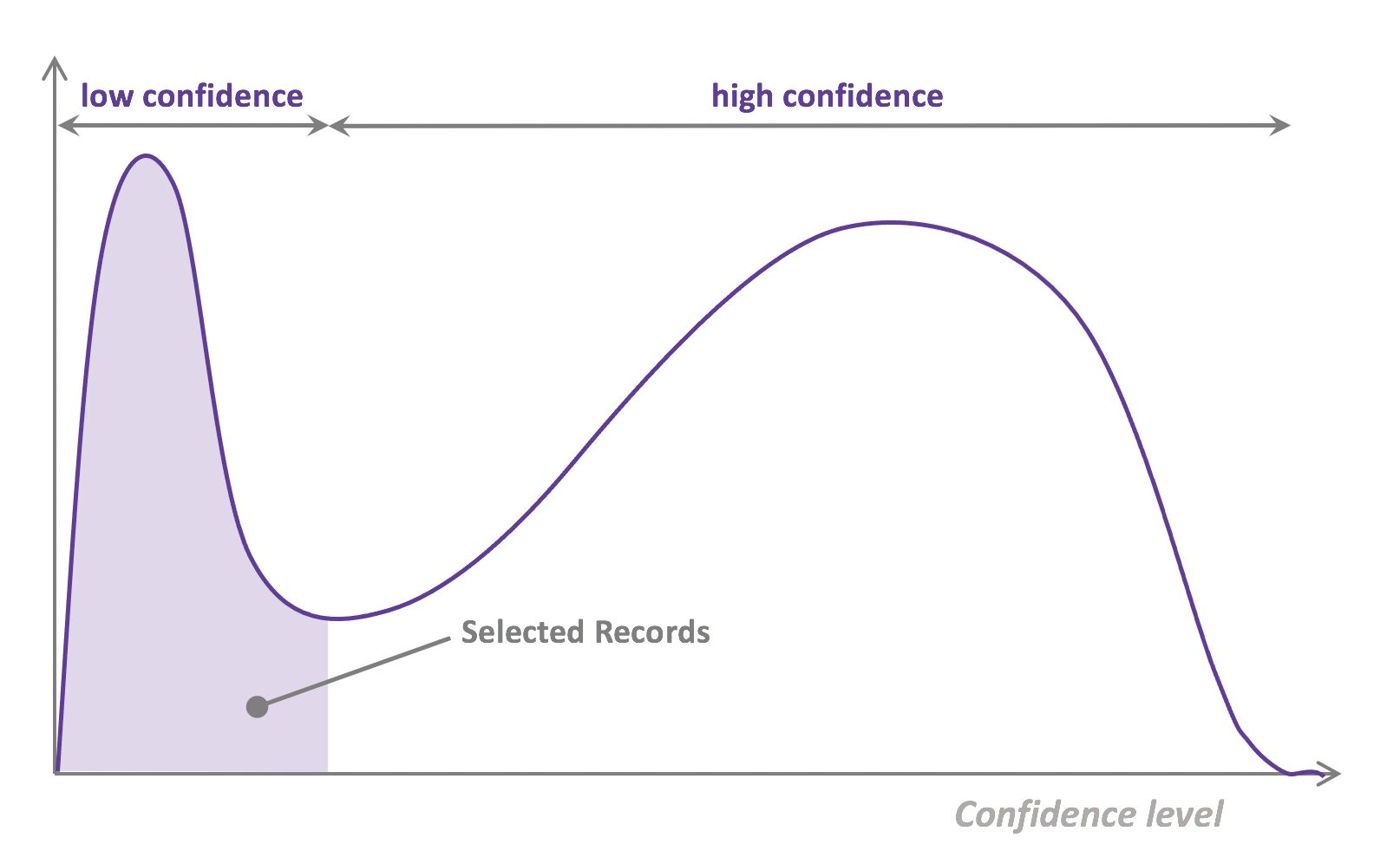
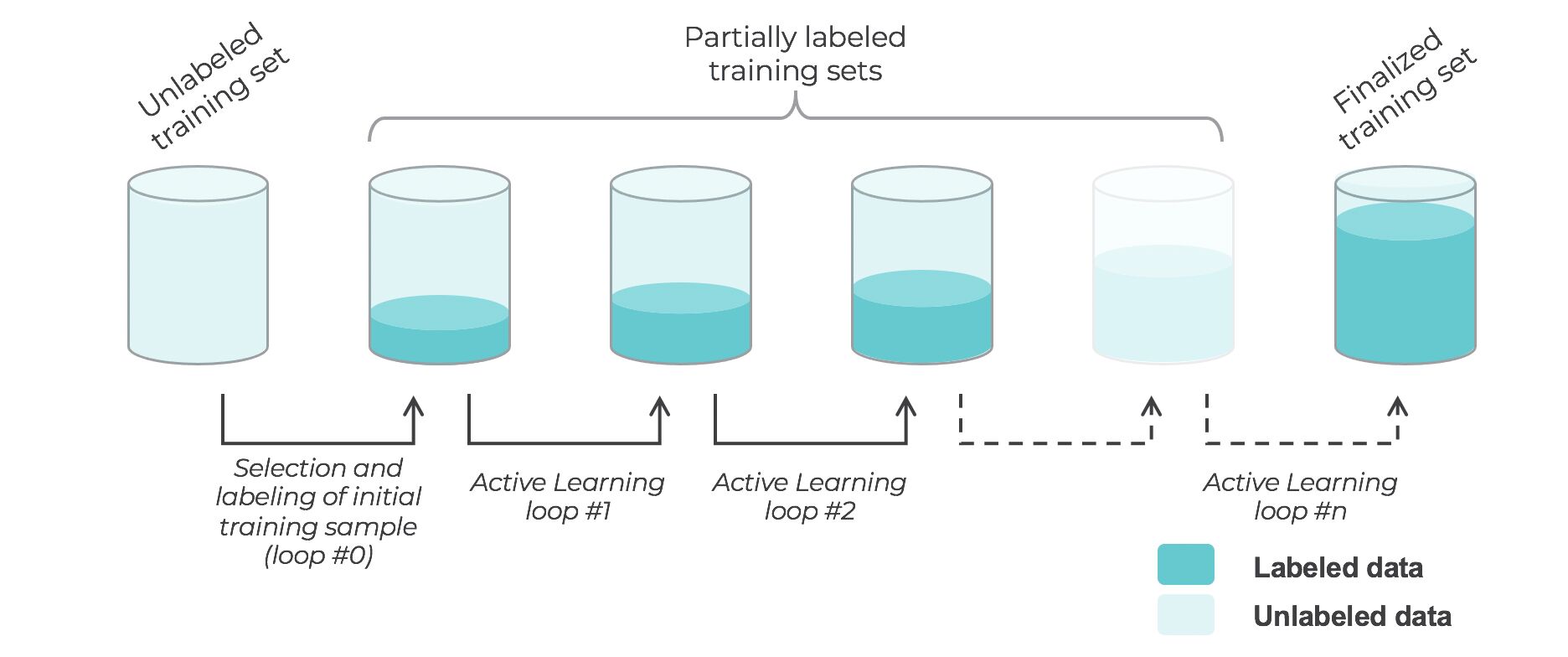
What are the types of active learning?
- There are many different “flavors” of active learning, but did you know that active learning could be broken down into two main categories, “streaming active learning”, and “pooling (batch) active learning”?
- Pooling Active Learning, is when all records available for training data have to be evaluated before a decision can be made about the ones to keep. For example, if your querying strategy is least-confidence, you goal is to select the N records that were predicted with the lowest confidence level in the previous loop, which means all records have to be ranked accordingly to their confidence level. Pooling Active Learning hence requires more compute resources for inference (the entire remainder of the dataset, at each loop, needs to be inferred), but provides a better control of loop sizes and the process as a whole.
- Streaming Active Learning, is when a decision is made “on the fly”, record by record. If your selection strategy was to select all records predicted with a confidence level lower than X% for the previous loop, you’d be doing Streaming AL. This technique obviously requires less compute, and can be used in combination with Online Learning, but it comes with a huge risk: there is no guarantee regarding the amount of data that will be selected. Set the threshold too low, and you won’t select any data for the next loop. Set the threshold too high, and all the remaining data gets selected, and you lose the benefit of AL.
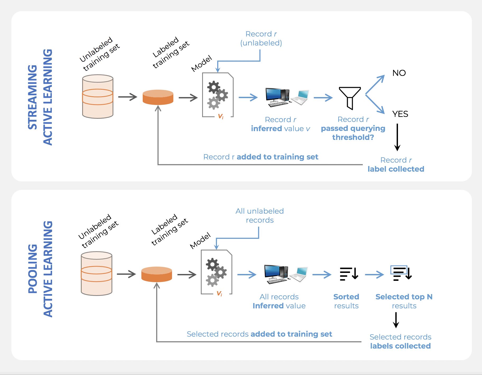
What is the difference between online learning and active learning?
- Online learning is essentially the concept of training a machine learning model on streaming data. In that case, data arrives little-by-little, sequentially, and the model is updated as opposed to be trained entirely from scratch.
- Active learning also consists in training a model sequentially, but the difference is that the training dataset is already fully available. Active learning simply selects small samples of data incrementally; the model is either retrained with the totality of selected records at a given point in time, or updated with the newly selected data.
- Online learning is required when models are to be trained at the point of collection (e.g, on the edge of a device), but active learning, just like supervised learning, usually involves the model being trained offline.
Why is active learning not frequently used with deep learning?
-
Active Learning was relatively popular among ML scientists during the pre-Deep Learning era, and somehow fell out of favor afterwards.
-
The reason why is actually relatively simple: Active Learning usually doesn’t work as well with Deep Learning Models (at least the most common querying strategies don’t). So people gave up on Deep Active Learning pretty quickly. The two most important reasons are the following:
-
The least-confidence, by far the most popular querying strategy, requires the computation of a confidence score. However, the softmax technique which most ML scientists rely on, is relatively unreliable (see this article for details to learn about a better way to compute confidence: https://arxiv.org/pdf/1706.04599.pdf)
-
Active learning, as a process, is actually meant to “grow” a better dataset dynamically. At each loop, more records are selected, which means the same model is retrained with incrementally larger data. However, many hyperparameters in neural nets are very sensitive to the amount of data used. For example, a certain number of epochs might lead to overfitting with early loops and underfitting later on. The proper way of doing Deep Active Learning would be to do hyperparameter tuning dynamically, which is rarely done.
What does active learning have to do with explore-exploit?
- Using the “uncertainty-based”/”least/lowest-confidence” querying strategy as a selection criteria in an active learning process could cause issues when working with a real-life (messy) dataset, as indicated above.
- Uncertainty-based active learning aims at selecting records based on how “certain” (or confident) the model already is about what it knows. Assuming the model can be trusted to self-evaluate properly, then:
- Selecting low confidence records is about picking what the model seems not to know yet; it is a pure exploration process.
- Selecting high confidence records is about picking what the model seems to already know, and that would be about reinforcing that knowledge; it is a pure exploitation process.
- While the “uncertainty-based”/”least/lowest-confidence” querying strategy strategy is the most common using active learning, it might be better to balance exploration and exploitation, and that active learning can and should, in fact, be formulated as a reinforcement learning problem.
What are the differences between a model that minimizes squared error and the one that minimizes the absolute error? and in which cases each error metric would be more appropriate?
- Both mean square error (MSE) and mean absolute error (MAE) measures the distances between vectors and express average model prediction in units of the target variable. Both can range from 0 to infinity, the lower they are the better the model.
- The main difference between them is that in MSE the errors are squared before being averaged while in MAE they are not. This means that a large weight will be given to large errors. MSE is useful when large errors in the model are trying to be avoided. This means that outliers affect MSE more than MAE (because large errors have a greater influence than small errors), that is why MAE is more robust to outliers.
- Computation-wise MSE is easier to use as the gradient calculation will be more straightforward than MAE, since MAE requires linear programming to calculate it.
Define tuples and lists in Python What are the major differences between them?
- Lists:
- In Python, a list is created by placing elements inside square brackets
[], separated by commas. A list can have any number of items and they may be of different types (integer, float, string, etc.). A list can also have another list as an item. This is called a nested list.- Lists are mutable (we can change, add, delete and modify stuff).
- Lists are better for performing operations, such as insertion and deletion.
- Lists consume more memory.
- Lists have several built-in methods.
- In Python, a list is created by placing elements inside square brackets
- Tuples:
- A tuple is a collection of objects which ordered and immutable. Tuples are sequences, just like lists. The differences between tuples and lists are, the tuples cannot be changed unlike lists and tuples use parentheses, whereas lists use square brackets.
- Tuples are immutable (we cannot change, add, delete and modify stuff).
- Tuple data type is appropriate for accessing the elements.
- Tuples consume less memory as compared to the list.
- Tuple does not have many built-in methods.
- A tuple is a collection of objects which ordered and immutable. Tuples are sequences, just like lists. The differences between tuples and lists are, the tuples cannot be changed unlike lists and tuples use parentheses, whereas lists use square brackets.
Given a left-skewed distribution that has a median of 60, what conclusions can we draw about the mean and the mode of the data?
- Left skewed distribution means the tail of the distribution is to the left and the tip is to the right. So the mean which tends to be near outliers (very large or small values) will be shifted towards the left or in other words, towards the tail.
- While the mode (which represents the most repeated value) will be near the tip and the median is the middle element independent of the distribution skewness, therefore it will be smaller than the mode and more than the mean.
- Thus,
- Mean < 60
- Mode > 60
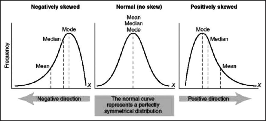
Explain the kernel trick in SVM and why we use it and how to choose what kernel to use?
- Kernels are used in SVM to map the original input data into a particular higher dimensional space where it will be easier to find patterns in the data and train the model with better performance.
- For e.g.: If we have binary class data which form a ring-like pattern (inner and outer rings representing two different class instances) when plotted in 2D space, a linear SVM kernel will not be able to differentiate the two classes well when compared to a RBF (radial basis function) kernel, mapping the data into a particular higher dimensional space where the two classes are clearly separable.
- Typically without the kernel trick, in order to calculate support vectors and support vector classifiers, we need first to transform data points one by one to the higher dimensional space, and do the calculations based on SVM equations in the higher dimensional space, then return the results. The ‘trick’ in the kernel trick is that we design the kernels based on some conditions as mathematical functions that are equivalent to a dot product in the higher dimensional space without even having to transform data points to the higher dimensional space. i.e we can calculate support vectors and support vector classifiers in the same space where the data is provided which saves a lot of time and calculations.
- Having domain knowledge can be very helpful in choosing the optimal kernel for your problem, however in the absence of such knowledge following this default rule can be helpful: For linear problems, we can try linear or logistic kernels and for nonlinear problems, we can use RBF or Gaussian kernels.
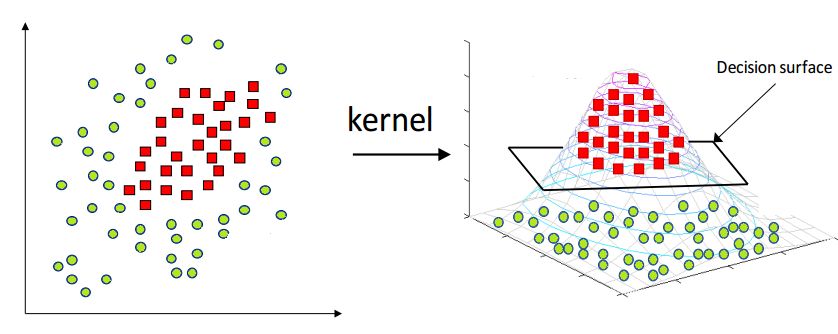
Can you explain the parameter sharing concept in deep learning?
- Parameter sharing is the method of sharing weights by all neurons in a particular feature map. Therefore helps to reduce the number of parameters in the whole system, making it computationally cheap. It basically means that the same parameters will be used to represent different transformations in the system. This basically means the same matrix elements may be updated multiple times during backpropagation from varied gradients. The same set of elements will facilitate transformations at more than one layer instead of those from a single layer as conventional. This is usually done in architectures like Siamese that tend to have parallel trunks trained simultaneously. In that case, using shared weights in a few layers (usually the bottom layers) helps the model converge better. This behavior, as observed, can be attributed to more diverse feature representations learned by the system. Since neurons corresponding to the same features are triggered in varied scenarios. Helps to model to generalize better.
- Note that sometimes the parameter sharing assumption may not make sense. This is especially the case when the input images to a ConvNet have some specific centered structure, where we should expect, for example, that completely different features should be learned on one side of the image than another.
- One practical example is when the input is faces that have been centered in the image. You might expect that different eye-specific or hair-specific features could (and should) be learned in different spatial locations. In that case, it is common to relax the parameter sharing scheme, and instead, simply call the layer a Locally-Connected Layer.
What is the difference between BETWEEN and IN operators in SQL?
BETWEEN–> range between two elements including themselves);IN–> elements in a set(list)- As an simple example:
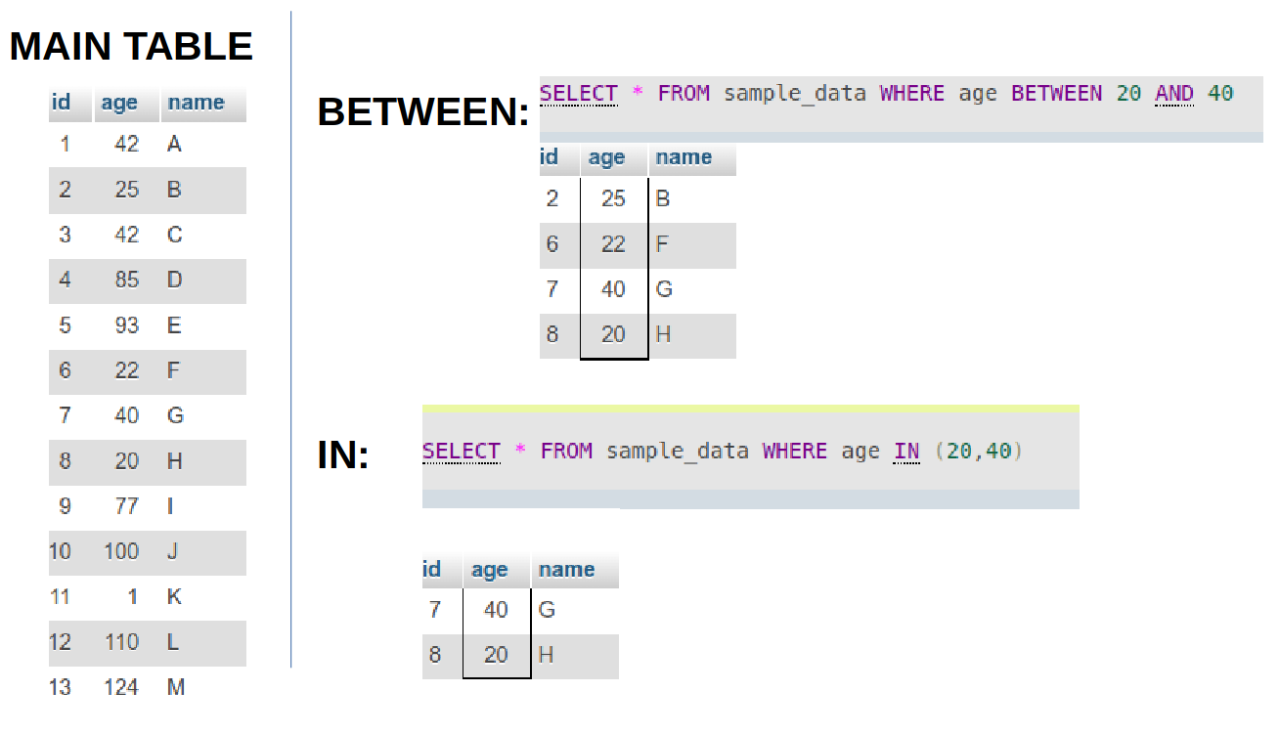
What is the meaning of selection bias and how to avoid it?
-
Sampling bias is the phenomenon that occurs when a research study design fails to collect a representative sample of a target population. This typically occurs because the selection criteria for respondents failed to capture a wide enough sampling frame to represent all viewpoints.
- The cause of sampling bias almost always owes to one of two conditions.
- Poor methodology: In most cases, non-representative samples pop up when researchers set improper parameters for survey research. The most accurate and repeatable sampling method is simple random sampling where a large number of respondents are chosen at random. When researchers stray from random sampling (also called probability sampling), they risk injecting their own selection bias into recruiting respondents.
- Poor execution: Sometimes data researchers craft scientifically sound sampling methods, but their work is undermined when field workers cut corners. By reverting to convenience sampling (where the only people studied are those who are easy to reach) or giving up on reaching non-responders, a field worker can jeopardize the careful methodology set up by data scientists.
- The best way to avoid sampling bias is to stick to probability-based sampling methods. These include simple random sampling, systematic sampling, cluster sampling, and stratified sampling. In these methodologies, respondents are only chosen through processes of random selection—even if they are sometimes sorted into demographic groups along the way.
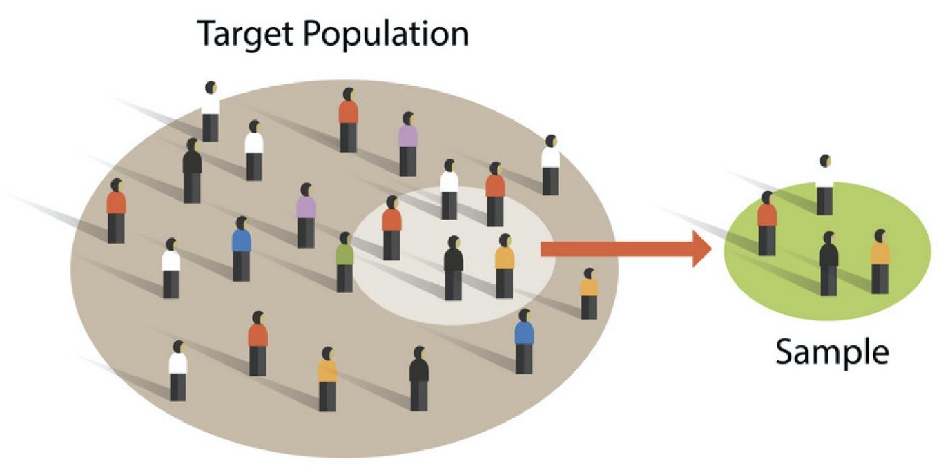
Given two python series, write a function to compute the euclidean distance between them?
- There are different ways to solve this question. The notebook snippet below shows various ways (along with credits to the respetive individual authors) and also shows the computation time for each method. Furthermore, the computation time for each method is calculated depending on whether the input was a NumPy array vs. Python Series and as shown using a NumPy array decreases the computation time.
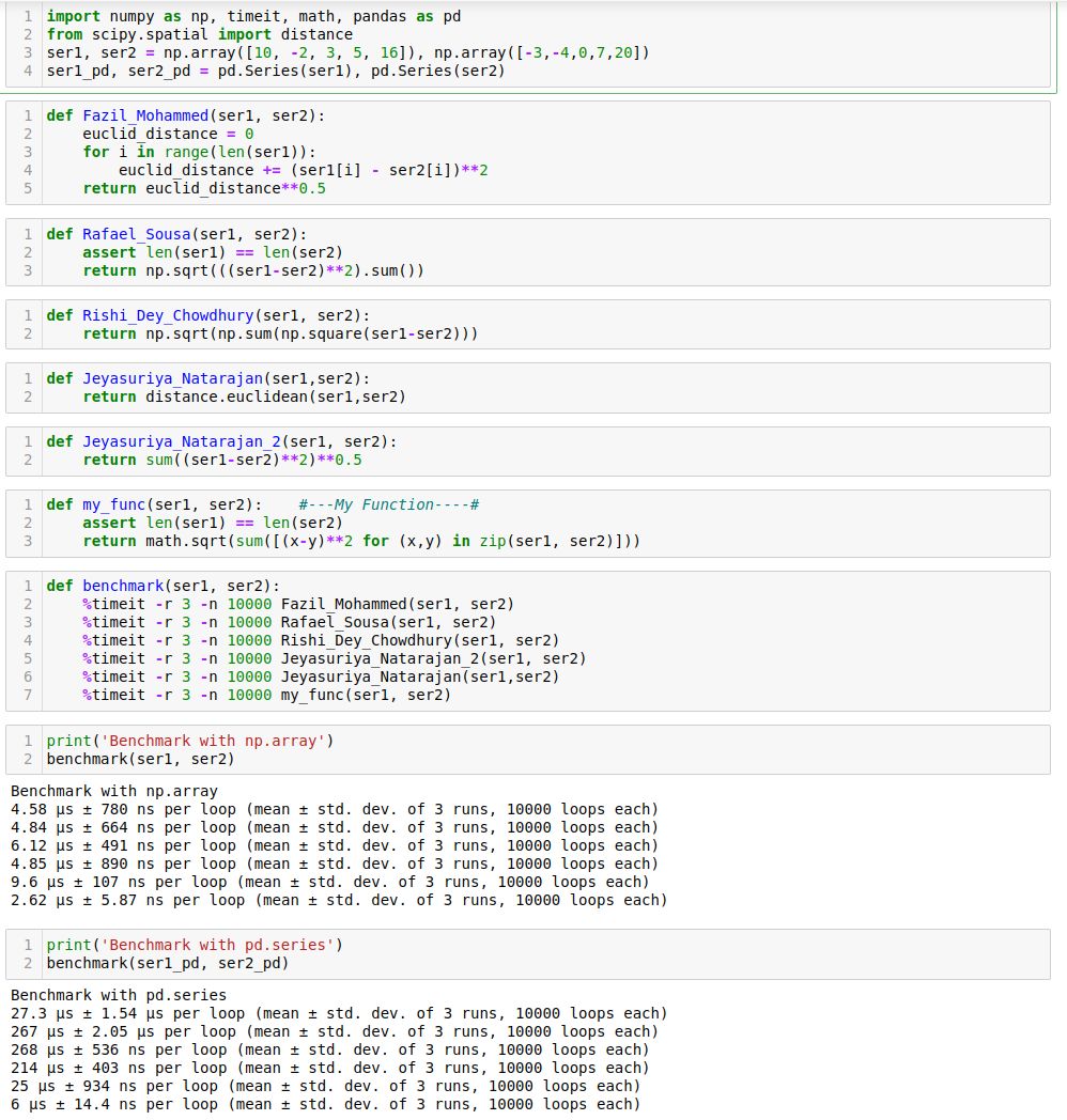
Define the cross-validation process and the motivation behind using it?
-
Cross-validation is a technique used to assess the performance of a learning model in several subsamples of training data. In general, we split the data into train and test sets where we use the training data to train our model and the test data to evaluate the performance of the model on unseen data and validation set for choosing the best hyperparameters. Now, a random split in most cases (for large datasets) is fine. But for smaller datasets, it is susceptible to loss of important information present in the data in which it was not trained. Hence, cross-validation though computationally bit expensive combats this issue.
-
The process of cross-validation is as the following:
- Define \(k\) or the number of folds.
- Randomly shuffle the data into \(k\) equally-sized blocks (folds).
- For each \(i\) in fold (1 to \(k\)), train the data using all the folds except for fold \(i\) and test on the fold \(i\).
- Average the \(k\) validation/test error from the previous step to get an estimate of the error.
- This process aims to accomplish the following:
- Prevent overfitting during training by avoiding training and testing on the same subset of the data points
- Avoid information loss by using a certain subset of the data for validation only. This is important for small datasets.
- Cross-validation is always good to be used for small datasets, and if used for large datasets the computational complexity will increase depending on the number of folds.
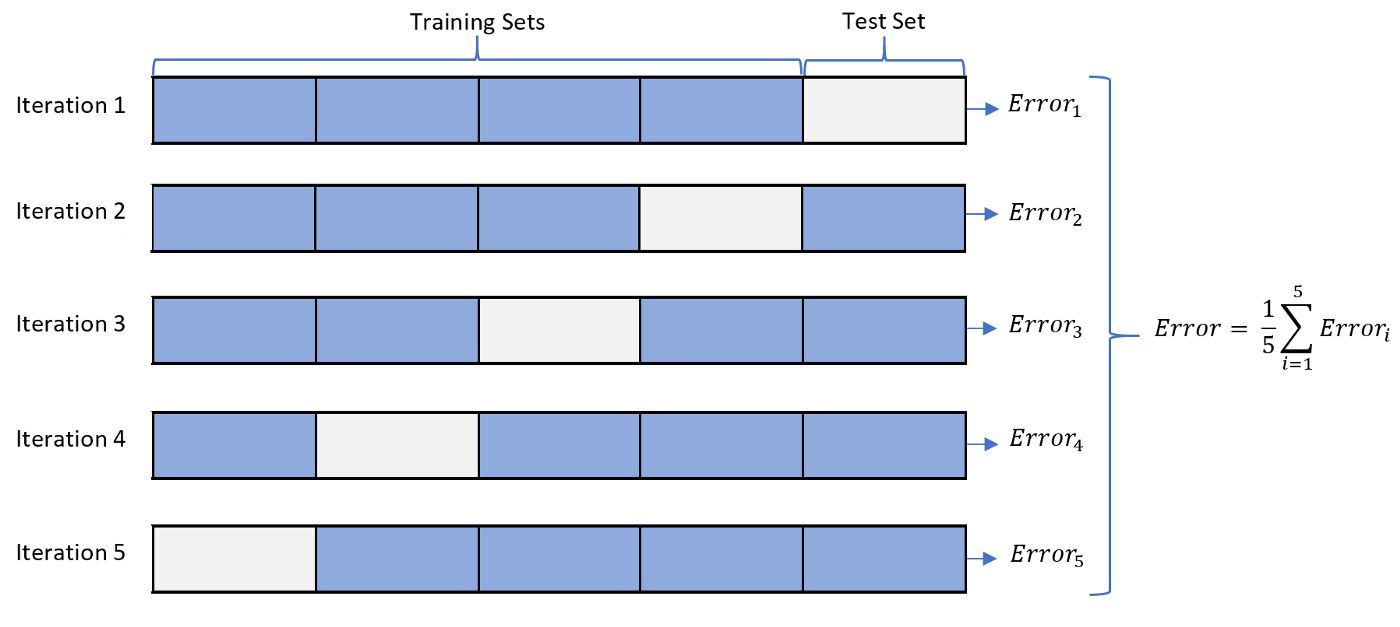
What is the difference between the Bernoulli and Binomial distribution?
- Bernoulli and Binomial are both types of probability distributions.
-
The function of Bernoulli is given by
\[p(x) =p^x * q^(1-x), x=[0,1]\]- where,
- Mean is \(p\).
- Variance \(p*(1-p)\).
- where,
-
The function Binomial is given by:
\[p(x) = nCx p^x q^(n-x) x=[0,1,2...n]\]- where,
- Mean: \(np\).
- Variance: \(npq\). Where p and q are the probability of success and probability of failure respectively, n is the number of independent trials and x is the number of successes.
- where,
- As we can see sample space (\(x\)) for Bernoulli distribution is Binary (2 outcomes), and just a single trial.
- For e.g., a loan sanction for a person can be either a success or a failure, with no other possibility. (Hence single trial).
- Whereas for Binomial the sample space (\(x\)) ranges from \(0-n\).
- As an example, tossing a coin 6 times, what is the probability of getting 2 or a few heads?
- Here sample space is \(x=[0,1,2]\) and more than 1 trial and \(n=6\) (finite).
- In short, Bernoulli Distribution is a single trial version of Binomial Distribution.
Given an integer \(n\) and an integer \(K\), output a list of all of the combinations of \(k\) numbers chosen from 1 to \(n\). For example, if \(n=3\) and \(k=2\), return \([1,2],[1,3],[2,3]\).
- There are different solutions one of them is the one below, there are other solutions in the comments of the original post and also the benchmarking between them thanks to Behnam Hedayat
from itertools import combinations
def find_combintaion(k, n):
	list_num = []
	comb = combinations([k for x in range (1, n+1)], k)
	for i in comb:
		list_num.append(i)

	print("(k: {}, n: {}):".format(k, n))
	print(list_num, "\n")
Explain the long-tailed distribution and provide three examples of relevant phenomena that have long tails. Why are they important in classification and regression problems?
- A long-tailed distribution is a type of heavy-tailed distribution that has a tail (or tails) that drop off gradually and asymptotically.
- Three examples of relevant phenomena that have long tails:
- Frequencies of languages spoken
- Population of cities
- Pageviews of articles
- All of these follow something close to the 80-20 rule: 80% of outcomes (or outputs) result from 20% of all causes (or inputs) for any given event. This 20% forms the long tail in the distribution.
- It’s important to be mindful of long-tailed distributions in classification and regression problems because the least frequently occurring values make up the majority of the population. This can ultimately change the way that you deal with outliers, and it also conflicts with some machine learning techniques with the assumption that the data is normally distributed.
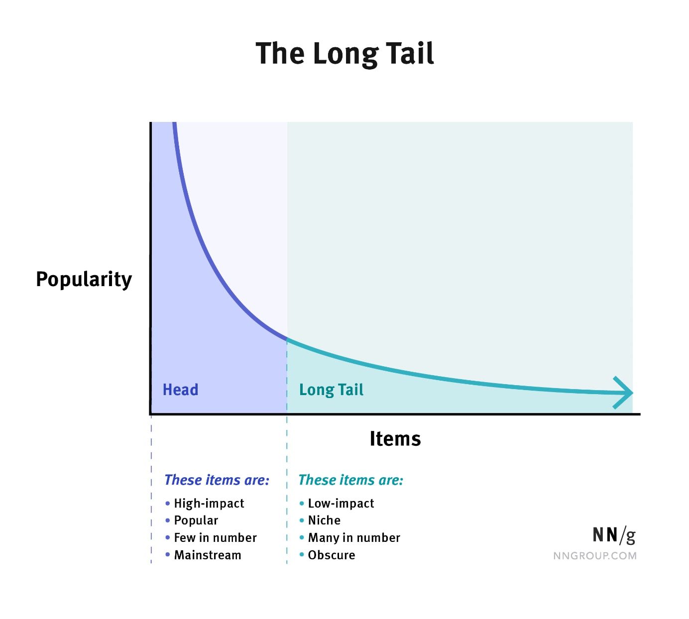
You are building a binary classifier and found that the data is imbalanced, what should you do to handle this situation?
- If there is a data imbalance there are several measures we can take to train a fairer binary classifier:
- Pre-Processing:
- Check whether you can get more data or not.
- Use sampling techniques (Up-sample minority class, downsample majority class, can take the hybrid approach as well). We can also use data augmentation to add more data points for the minority class but with little deviations/changes leading to new data points which are similar to the ones they are derived from. The most common/popular technique is SMOTE (Synthetic Minority Oversampling technique)
- Suppression: Though not recommended, we can drop off some features directly responsible for the imbalance.
- Learning Fair Representation: Projecting the training examples to a subspace or plane minimizes the data imbalance.
- Re-Weighting: We can assign some weights to each training example to reduce the imbalance in the data.
- In-Processing:
- Regularizaion: We can add score terms that measure the data imbalance in the loss function and therefore minimizing the loss function will also minimize the degree of imbalance with respect to the score chosen which also indirectly minimizes other metrics which measure the degree of data imbalance.
- Adversarial Debiasing: Here we use the adversarial notion to train the model where the discriminator tries to detect if there are signs of data imbalance in the predicted data by the generator and hence the generator learns to generate data that is less prone to imbalance.
- Post-Processing:
- Odds-Equalization: Here we try to equalize the odds for the classes w.r.t. the data is imbalanced for correct imbalance in the trained model. Usually, the F1 score is a good choice, if both precision and recall scores are important
- Choose appropriate performance metrics. For example, accuracy is not a correct metric to use when classes are imbalanced. Instead, use precision, recall, F1 score, and ROC curve.
- Pre-Processing:
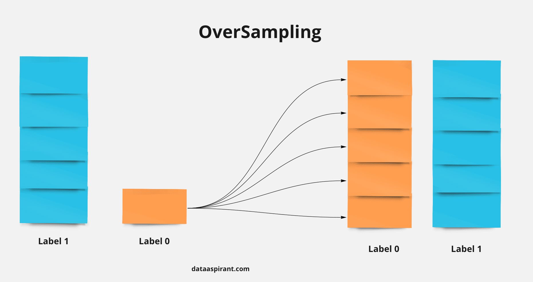
What to do with imbalance class
- Dealing with imbalanced classes is a common challenge in machine learning, where the number of instances in one class significantly outweighs the number of instances in another class. This issue can negatively impact the performance and accuracy of the machine learning model, as it tends to favor the majority class.
- Some common issues associated with imbalanced classes are:
- Biased Model: The model may favor the majority class, leading to low recall or sensitivity for the minority class, which can be problematic in scenarios where detecting the minority class is critical.
- Poor Generalization: Imbalanced data can hinder the model’s ability to generalize well to unseen data, as it may not adequately capture the underlying patterns of the minority class.
- Evaluation Metrics: Traditional accuracy may not be an appropriate evaluation metric, as a model predicting only the majority class can still achieve high accuracy in an imbalanced setting. Alternative metrics like precision, recall, F1-score, and area under the Receiver Operating Characteristic (ROC) curve are more suitable.
- Resampling Techniques:
- Undersampling: Randomly remove samples from the majority class to balance the class distribution.
- Oversampling: Create synthetic samples in the minority class to increase its representation.
- SMOTE (Synthetic Minority Over-sampling Technique): Generate synthetic samples by interpolating between existing minority class samples.
- ADASYN (Adaptive Synthetic Sampling): Similar to SMOTE, but gives more emphasis to difficult-to-learn minority samples.
- Class Weighting:
- Assign higher weights to the minority class during model training to penalize misclassifications and encourage better classification of the minority class.
- Ensemble Methods:
- Combine multiple models trained on different subsets of the data or using different algorithms to improve overall performance and handle class imbalance.
- Anomaly Detection:
- Treat the minority class as an anomaly and use techniques such as One-Class SVM or Isolation Forest to detect and classify instances of the minority class.
- Collect More Data:
- If possible, collect additional data for the minority class to improve its representation and address the class imbalance problem.
- Evaluation Metrics:
- Instead of solely relying on accuracy, consider using evaluation metrics that are robust to imbalanced classes, such as precision, recall, F1-score, area under the ROC curve (AUC-ROC), or precision-recall curve.
It’s important to note that the choice of approach depends on the specific problem, dataset, and the underlying reasons for class imbalance. Experimentation and careful evaluation of different techniques are necessary to find the most effective solution.
By employing these techniques and adapting them to the specific problem at hand, we can mitigate the impact of imbalanced classes and improve the overall performance and fairness of our machine learning models.
If there are 30 people in a room, what is the probability that everyone has different birthdays?
- The sample space is 365^30 and the number of events is \(365_p_30\) because we need to choose persons without replacement to get everyone to have a unique birthday therefore the Prob = \(365_p_30\) / 365^30 = 0.2936
- Interesting facts provided by Rishi Dey Chowdhury:
- With just 23 people there is over 50% chance of a birthday match and with 57 people the match probability exceeds 99%. One intuition to think of why with such a low number of people the probability of a match is so high. It’s because for a match we require a pair of people and 23 choose 2 is 23*11 = 253 which is a relatively big number and ya 50% sounds like a decent probability of a match for this case.
- Another interesting fact is if the assumption of equal probability of birthday of a person on any day out of 365 is violated and there is a non-equal probability of birthday of a person among days of the year then, it is even more likely to have a birthday match.
- A theoretical explanation is provided in the figure below thanks to Fazil Mohammed.
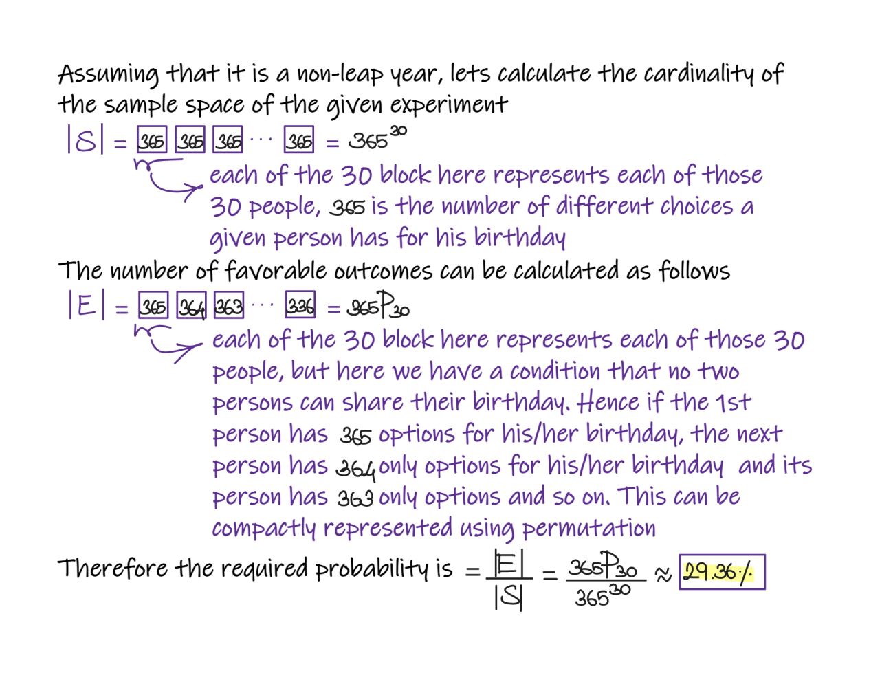
What is the Vanishing Gradient Problem and how do you fix it?
- The vanishing gradient problem is encountered in artificial neural networks with gradient-based learning methods and backpropagation. In these learning methods, each of the weights of the neural network receives an update proportional to the partial derivative of the error function with respect to the current weight in each iteration of training. Sometimes when gradients become vanishingly small, this prevents the weight to change value.
- When the neural network has many hidden layers, the gradients in the earlier layers will become very low as we multiply the derivatives of each layer. As a result, learning in the earlier layers becomes very slow. This can cause the network to stop learning. This problem of vanishing gradients happens when training neural networks with many layers because the gradient diminishes dramatically as it propagates backward through the network.
- Some ways to fix it are:
- Use skip/residual connections.
- Using ReLU or Leaky ReLU over sigmoid and tanh activation functions.
- Use models that help propagate gradients to earlier time steps such as GRUs and LSTMs.
What are Residual Networks? How do they help with vanishing gradients?
- Here is a concept that you should know whether you are trying to get a job in AI or you want to improve your knowledge of AI: residual networks.
- Skip connections or residual networks feed the output of a layer to the input of the subsequent layers, skipping intermediate operations.
- They appear in the Transformer architecture, which is the base of GPT4 and other language models, and in most computer vision networks.
- Residual connections have several advantages:
- They reduce the vanishing gradient since the gradient value is transferred through the network.
- They allow later layers to learn from features generated in the initial layers. Without the skip connection, that initial info would be lost.
- They help to maintain the gradient surface smooth and without too many saddle points.
- This keeps gradient descent to get stuck in local minima, in other words, the optimization process is more robust and then we can use deeper networks.
- ResNet paper was published at the end of 2015 and was very influential because, for the first time, a network with 152 layers surpassed the human performance in image classification.
- Deep learning is based on two competing forces: the more layers, the higher the generalization power of the network, however, the more layers, the more difficult is to optimize.
- In other words, the deeper the network, the better it models the real world in theory, however, it is very difficult to train in practice.
- ResNet was a very important step to solve this problem.
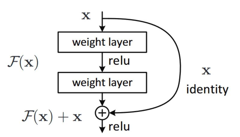
How does ResNet-50 solve the vanishing gradients problem of VGG-16?
- During the ImageNet Large Scale Visual Recognition Challenge (ILSVRC) that with the increase in the number of layers the deep learning models will perform better because of more parameters. However, because of more number of layers, there was a problem with vanishing gradients. In fact, the authors of ResNet, in the original paper, noticed that neural networks without residual connections don’t learn as well as ResNets, although they are using batch normalization, which, in theory, ensures that gradients should not vanish.
- Enter ResNet that utilize skip connections under-the-hood.
- The skip connections allow information to skip layers, so, in the forward pass, information from layer l can directly be fed into layer $l+t$ (i.e., the activations of layer $l$ are added to the activations of layer $l+t$, for $t >= 2$ and, during the forward pass, the gradients can also flow unchanged from layer $l+t$ to layer $l$. This prevents the vanishing gradient problem (VGP). Let’s explain how.
- The VGP occurs when the elements of the gradient (the partial derivatives with respect to the parameters of the network) become exponentially small, so that the update of the parameters with the gradient becomes almost insignificant (i.e., if you add a very small number $0 < \epsilon « 1$ to another number $d$, $d+\epsilon$ is almost the same as d and, consequently, the network learns very slowly or not at all (considering also numerical errors).
- Given that these partial derivatives are computed with the chain rule, this can easily occur, because you keep on multiplying small (finite-precision) numbers.
- The deeper the network, the more likely the VGP can occur. This should be quite intuitive if you are familiar with the chain rule and the back-propagation algorithm (i.e. the chain rule).
- By allowing information to skip layers, layer l+t receives information from both layer $l+t−1$ and layer $l$ (unchanged, i.e., you do not perform multiplications).
- From the paper: “Our results reveal one of the key characteristics that seem to enable the training of very deep networks: Residual networks avoid the vanishing gradient problem by introducing short paths which can carry gradient throughout the extent of very deep networks.”
How do you run a deep learning model efficiently on-device?
- Let’s take the example of LLaMA, a ChatGPT-like LLM by Meta.
- You can run one of the latest LLMs if you have a computer with 4Gb of RAM.
- The model is implemented in C++ (with Python wrappers) and uses several optimization techniques:
- Quantization
- Quantization represents the weights of the model in a low-precision data type like 4-bit integer (INT4) instead of the usual 32-bit floating precision (FP32).
- For example, the smallest LLaMA model has 7B parameters.
- The original model uses 13GB of RAM, while the optimized model uses 3.9GB.
- Faster weight loading
- Another optimization is to load the model weights using
mmap()instead of standard C++ I/O. - That enabled to load LLaMA 100x faster using half as much memory.
mmap()maps the read-only weights usingMAP_SHARED, which is the same technique that’s traditionally used for loading executable software.
- Another optimization is to load the model weights using
- Quantization
When are tress not useful?
- Use tree ensembles (random forest/gradient boosted trees) unless you have a reason not to.
- Here are some of the only reasons not to use tree ensembles for your supervised machine learning problem:
- You are working with unstructured data (text, image, audio, video)
- You are doing statistical inference on a parametric model to draw conclusions (for example, causal inference)
- You have strict interpretability requirements from a legal perspective
- You are trying to model a phenomenon with a known relationship in order to extrapolate the relationship (for example, logistic curves to model population growth scenarios)
- You have very restrictive latency and/or memory requirements (sparse linear models and SVMs are superior here)
- Ignoring these, tree ensembles are typically more adaptable and performant. Spend less time trying to beat them, and more time iterating on data quality, feature engineering, and MLOps best practices.

Misc
What is the difference between standardization and normalization?
- Normalization means rescaling the values into a range of (typically) [0,1].
- Standardization refers to centering the values around the mean with a unit standard deviation.
When do you standardize or normalize features?
- Rule of thumb:
- Standardization, when the data follows a Gaussian distribution and your algorithm assumes your data follows a Gaussian Distribution like Linear Regression.
- Normalization, when your data has varying scales and your algorithm doesn’t make assumptions about the distribution of your data like KNN.
Why is relying on the mean to make a business decision based on data statistics a problem?
- There is a famous joke in Statistics which says that, “if someone’s head is in the freezer and leg is in the oven, the average body temperature would be fine, but the person may not be alive”.
- Making decisions solely based on mean value is not advisable. The issue with mean is that it is affected significantly by the presence of outliers, and may not be the correct central representation of the dataset.
- It is thus advised that the mean should be used along with other measures and measures of variability for better understanding and explainability of the data.

Explain the advantages of the parquet data format and how you can achieve the best data compression with it?
-
The parquet format is something that every data person has to be aware about. Its a popular choice for data storage for faster query and better compression but do you know how the sorting order can be very important when we optimize for compression?
-
Parquet uses columnar storage, which means that data is stored by column rather than by row. This can lead to significant improvements in compression, because values in a column tend to be more homogeneous than values in a row. However, to achieve the best compression, it’s important to sort the data within each column in a specific way.
-
Parquet uses a technique called “run-length encoding” (RLE) to compress repetitive sequences of values within a column. RLE works by storing a value once, followed by a count of how many times that value is repeated. For example, if a column contains the values [1,1, 1, 1, 2, 2, 3, 3, 3, 3, 3], RLE would store it as [1, 4, 2, 2, 3, 5].
-
To take advantage of RLE, it’s important to sort the data within each column in a way that maximizes the number of repetitive sequences. For example, if a column contains the values [1, 2, 3, 4, 5, 1, 2, 3, 4, 5], sorting it as [1, 1, 2, 2, 3, 3, 4, 4, 5, 5] would result in better compression.
-
In addition to RLE, Parquet also uses other compression techniques such as dictionary encoding and bit-packing to achieve high compression ratios. These techniques also benefit from sorted data, as they can take advantage of the repetition and predictability of sorted values to achieve better compression.
-
What about the order of sorting when we sort on multiple columns, does that have an impact ? The asnwer is yes. Sorting the data by the most significant column(s) first can lead to better compression because it can group similar values together, allowing for better compression within each data page.
-
For example, consider a dataset with three columns: column1, column2 and column3. If most of the values in column1 are the same or similar (lower cardinality), then sorting the data by column1 first can help group together similar values and achieve better compression within each data page.
-
In summary, the sorting order of data can have a significant impact on data compression in Parquet and should be considered for data pipelines.
What is Redis?
- Redis is not just a key-value cache - it can be used as a database, as a pub-sub, and much more.
-
“Redis” actually stands for “Remote DIctionary Server”. Redis was originally designed as a key-value store database for remote access, with a focus on speed, simplicity, and versatility.
-
Since Redis’ code is open source, you can deploy Redis yourself. There are many ways of Redis deployment: standalone mode, cluster mode, sentinel mode, and replication mode.
-
In Redis, the most popular mode of deployment is cluster mode. Redis Cluster is a distributed implementation of Redis, in which data is partitioned and distributed across multiple nodes in a cluster.
-
In Redis Cluster, each node is responsible for a subset of the keyspace, and multiple nodes work together to form a distributed system that can handle large amounts of data and high traffic loads. The partitioning of data is based on hashing of the key, and each node is responsible for a range of hash slots.
-
The hash slot range is distributed evenly among the nodes in the cluster, and each node is responsible for storing and serving data for the hash slots assigned to it. When a client sends a request to a node, the node checks the hash slot of the requested key, and if the slot is owned by the node, the request is processed locally. Otherwise, the request is forwarded to the node that owns the slot.
-
Redis Cluster also provides features for node failover, in which if a node fails, its hash slot range is automatically taken over by another node in the cluster. This ensures high availability and fault tolerance in the system.
- Overall, in clustered Redis, data is arranged based on a consistent hashing algorithm, where each node is responsible for a subset of the keyspace and works together to form a distributed system that can handle large amounts of data and traffic loads.
MLOps
- Machine learning (ML) systems, like any software systems, require reliable development and operation practices to ensure scalability. However, ML systems possess distinctive characteristics that set them apart from traditional software systems (source):
- Team Skills: ML projects involve data scientists or ML researchers who focus on data analysis, model development, and experimentation. These team members may lack experience in building production-ready services as software engineers do.
- Development: ML is inherently experimental, necessitating the exploration of various features, algorithms, modeling techniques, and parameter configurations to identify optimal solutions promptly. The challenge lies in tracking successful approaches, maintaining reproducibility, and maximizing code reusability.
- Testing: Testing ML systems goes beyond typical unit and integration testing. It requires data validation, evaluation of trained model quality, and validation of the entire model. Additional efforts are needed to ensure the correctness and performance of ML models.
- Deployment: Deploying an ML system involves more than simply releasing an offline-trained model as a prediction service. It often requires deploying a multi-step pipeline that automates retraining and model deployment. This adds complexity and necessitates automating tasks that were previously performed manually by data scientists.
- Production: ML models can experience performance degradation due to suboptimal coding and evolving data profiles. Models can deteriorate in various ways, requiring tracking of data summary statistics and monitoring online model performance to detect deviations and take appropriate action.
- While ML and other software systems share common practices such as continuous integration, unit testing, integration testing, and continuous delivery, there are notable differences:
- Continuous integration (CI) expands beyond testing and validating code and components to encompass data, data schemas, and models.
- Continuous delivery (CD) involves not only deploying a single software package or service but also automating the deployment of an ML training pipeline and subsequent model prediction services.
- Continuous training (CT) is a unique aspect of ML systems that involves automatic retraining and serving of models.
Data Science Workflow for Machine Learning
- In every machine learning (ML) project, once the business use case is defined and success criteria are established, the process of delivering an ML model to production follows a set of steps. These steps can be performed manually or automated through a pipeline.(source)
- Data Extraction: Relevant data from various sources is selected and integrated for the ML task at hand.
- Data Analysis: Exploratory data analysis (EDA) is conducted to gain insights into the available data for building the ML model. This involves understanding the data schema and characteristics required by the model, as well as identifying necessary data preparation and feature engineering steps.
- Data Preparation: The data is prepared for the ML task, including data cleaning, splitting the data into training, validation, and test sets, and applying transformations and feature engineering specific to the target task. The output of this step is a set of prepared data splits.
- Model Training: Different algorithms are implemented and trained on the prepared data to create various ML models. Additionally, hyperparameter tuning is applied to optimize the performance of the implemented algorithms. The output of this step is a trained ML model.
- Model Evaluation: The trained model is evaluated on a holdout test set to assess its quality and performance. This step produces a set of metrics used to evaluate the model’s effectiveness.
- Model Validation: The model is validated to ensure it meets deployment requirements and exhibits predictive performance superior to a predetermined baseline.
- Model Serving: The validated model is deployed to a target environment to serve predictions. Deployment options include microservices with a REST API for online predictions, embedding the model into edge or mobile devices, or integrating it into a batch prediction system.
- Model Monitoring: The model’s predictive performance is continuously monitored to identify potential issues and trigger iterations within the ML process.
- The level of automation applied to these steps determines the maturity of the ML process and influences the ability to train new models using new data or implementations. Below, we will see different levels of MLOps architecture as represented in (Google’s blog.).
MLOps level 0: Manual process
- At the basic level of maturity (Level 0) in ML model development and deployment, many teams rely on the expertise of data scientists and ML researchers to manually build and deploy models.
- This manual process lacks automation and follows a workflow outlined in the image below (source).

MLOps level 1: ML pipeline automation
- The image below and the content here is inspired by (Google’s blog.)

- Characteristics of MLOps Level 1 Setup:
- Rapid experiment: ML experiment steps are automated, allowing for quick iteration and readiness for production deployment.
- Continuous training (CT) of the model in production: The model is automatically trained using fresh data triggered by the live pipeline, ensuring ongoing model improvement.
- Experimental-operational symmetry: The same pipeline implementation used in the development environment is used in the preproduction and production environments, aligning with MLOps practices for unifying DevOps.
- Modularized code for components and pipelines: ML pipelines require reusable and composable components. Source code for components should be modularized, allowing for easy sharing and containerization to decouple execution environments and ensure reproducibility.
- Continuous delivery of models: ML pipelines in production continuously deliver prediction services using newly trained models on updated data. The deployment of the trained and validated models as prediction services is automated.
- Pipeline deployment: In Level 1, the entire training pipeline is deployed to production, with the pipeline running automatically and recurrently to serve the trained model as the prediction service.
- Additional Components:
- Data and model validation: Automated data and model validation steps are included in the production pipeline. Data validation ensures the data meets the expected schema, identifying schema skews and data value skews that may require retraining. Model validation evaluates the performance and consistency of the newly trained model before promotion to production.
- Feature store: A feature store, as an optional component, centralizes the storage and access of features for training and serving. It helps with feature reuse, maintaining consistency, and avoiding training-serving skew by providing up-to-date feature values.
- Metadata management: ML metadata is recorded to track pipeline execution, aid reproducibility, debug errors, and compare performance. It includes pipeline and component versions, execution details, parameter arguments, intermediate outputs, and evaluation metrics.
- ML pipeline triggers: ML production pipelines can be triggered in different ways, including on-demand, scheduled, availability of new training data, model performance degradation, and significant changes in data distributions (concept drift).
- Challenges:
- While the Level 1 setup accommodates manual testing and deployment of new pipeline implementations, it becomes challenging when multiple ML pipelines need to be managed, and frequent deployment of new implementations and ML ideas is required. In such cases, adopting a CI/CD setup becomes essential to automate the build, testing, and deployment of ML pipelines.
MLOps level 2: CI/CD pipeline automation
- To ensure a fast and dependable update of production pipelines, the integration of a robust automated CI/CD system is crucial. This system empowers data scientists to quickly experiment with new concepts related to feature engineering, model architecture, and hyperparameters. They can implement these ideas and automate the process of building, testing, and deploying new pipeline components to the designated environment.
- The accompanying diagram illustrates the implementation of an ML pipeline using CI/CD, combining the characteristics of an automated ML pipeline setup with automated CI/CD routines.
- The image below and the content here is inspired by (Google’s blog.)

- “This MLOps setup includes the following components:
- Source control
- Test and build services
- Deployment services
- Model registry
- Feature store
- ML metadata store
- ML pipeline orchestrator” (source)
- The diagram presented below depicts the stages of the ML CI/CD automation pipeline: (source) illustrates these characteristics that we will look further into below.

- Stages of the CI/CD automated ML pipeline.
- The pipeline comprises the following stages:
- Development and experimentation: Iteratively exploring new ML algorithms and modeling techniques, where the experiment steps are coordinated. The result of this stage is the source code for the ML pipeline steps, which are then stored in a source repository.
- Pipeline continuous integration: Building the source code and conducting various tests. The outputs of this stage are pipeline components (packages, executables, and artifacts) to be utilized in subsequent stages.
- Pipeline continuous delivery: Deploying the artifacts generated in the CI stage to the target environment. The outcome of this stage is a deployed pipeline featuring the new model implementation.
- Automated triggering: Automatically executing the pipeline in production, either according to a predefined schedule or triggered by specific events. The output of this stage is a trained model that is stored in the model registry.
- Model continuous delivery: Serving the trained model as a prediction service for generating predictions. The outcome of this stage is a deployed model prediction service.
- Monitoring: Collecting statistics on the model’s performance based on live data. The output of this stage serves as a trigger for executing the pipeline or initiating a new cycle of experimentation.
- It’s important to note that the data analysis step is still a manual process for data scientists before the pipeline begins a new iteration of the experiment. Similarly, the model analysis step also requires manual intervention.
- The pipeline comprises the following stages:
- Continuous integration
- This involves building, testing, and packaging the ML pipeline and its components whenever new code is committed or pushed to the source code repository. This process includes unit testing for feature engineering logic, different methods implemented in the model, convergence of model training, prevention of NaN values, and verification of artifact production and pipeline integration.
- “Unit testing your feature engineering logic.
- Unit testing the different methods implemented in your model. For example, you have a function that accepts a categorical data column and you encode the function as a one-hot feature.
- Testing that your model training converges (that is, the loss of your model goes down by iterations and overfits a few sample records).
- Testing that your model training doesn’t produce NaN values due to dividing by zero or manipulating small or large values.
- Testing that each component in the pipeline produces the expected artifacts.
- Testing integration between pipeline components.”(source)
- Continuous delivery
- This focuses on continuously delivering new pipeline implementations to the target environment, which enables the delivery of prediction services for the newly trained model. It involves verifying model compatibility with the target infrastructure, testing the prediction service and its performance, validating data for retraining or batch prediction, ensuring models meet performance targets, and deploying to test, pre-production, and production environments.
- “Verifying the compatibility of the model with the target infrastructure before you deploy your model. For example, you need to verify that the packages that are required by the model are installed in the serving environment, and that the memory, compute, and accelerator resources that are available.
- Testing the prediction service by calling the service API with the expected inputs, and making sure that you get the response that you expect. This test usually captures problems that might occur when you update the model version and it expects a different input.
- Testing prediction service performance, which involves load testing the service to capture metrics such as queries per seconds (QPS) and model latency.
- Validating the data either for retraining or batch prediction.
- Verifying that models meet the predictive performance targets before they are deployed.
- Automated deployment to a test environment, for example, a deployment that is triggered by pushing code to the development branch.
- Semi-automated deployment to a pre-production environment, for example, a deployment that is triggered by merging code to the main branch after reviewers approve the changes.
- Manual deployment to a production environment after several successful runs of the pipeline on the pre-production environment.” (source)
- Implementing ML in a production environment goes beyond deploying a prediction API; it requires deploying an ML pipeline that automates retraining and deployment of new models. By setting up a CI/CD system, you can automate the testing and deployment of pipeline implementations, allowing you to adapt to changes in data and the business environment. You can gradually adopt these practices to enhance the automation of ML system development and production.
Bagging vs Boosting
- Bagging and boosting are two popular ensemble learning techniques used in machine learning to improve the performance of predictive models by combining multiple weaker models. While they have similar goals, they differ in their approach and how they create the ensemble.
- Ensemble learning is a powerful approach that combines multiple models to improve the predictive performance of machine learning algorithms. By leveraging the diversity of these models, ensemble learning helps mitigate the issues of bias, variance, and noise commonly encountered in individual models. It achieves this by training a set of classifiers or experts and allowing them to vote or contribute to the final prediction or classification.
- Bagging and boosting are two types of ensemble learning techniques that aim to decrease the variance and bias of a model, respectively. They combine multiple models to produce a more stable and accurate final model compared to a single classifier.
Bootstrapping
- Before diving into the specifics of bagging and boosting, let’s first understand bootstrapping. Bootstrapping is a sampling technique that involves creating subsets of observations from the original dataset with replacement.
- Each subset has the same size as the original dataset, and the random sampling allows us to better understand the bias and variance within the dataset. It helps estimate the mean and standard deviation by resampling from the dataset.
Bagging
- Bagging, short for Bootstrap Aggregation, is a straightforward yet powerful ensemble method. It applies the bootstrap procedure to high-variance machine learning algorithms, typically decision trees. The idea behind bagging is to combine the results of multiple models, such as decision trees, to obtain a more generalized and robust prediction. It creates subsets (bags) from the original dataset using random sampling with replacement, and each subset is used to train a base model or weak model independently. These models run in parallel and are independent of each other.
- The final prediction is determined by combining the predictions from all the models, often through averaging or majority voting.
Boosting
- Boosting is a sequential process where each subsequent model attempts to correct the errors made by the previous model. Unlike bagging, boosting involves training learners sequentially, with early learners fitting simple models to the data and subsequent learners analyzing the data for errors. The goal is to solve for net error from the prior model by adjusting the weights assigned to each data point. Boosting assigns higher weights to misclassified data points, so subsequent learners focus more on these difficult cases.
- Through this iterative process, boosting aims to convert a collection of weak learners into a stronger and more accurate model. The final model, often referred to as a strong learner, is a weighted combination of all the models.
Bagging vs Boosting
- Bagging and Boosting are both ensemble learning techniques used to improve the performance of machine learning models. However, they differ in their approach and objectives. Here are the key differences between Bagging and Boosting:
- Data Sampling:
- Bagging: In Bagging (short for Bootstrap Aggregating), multiple training datasets are created by randomly sampling from the original dataset with replacement. Each dataset is of the same size as the original dataset.
- Boosting: In Boosting, the training datasets are also created by random sampling with replacement. However, each new dataset gives more weight to the instances that were misclassified by previous models. This allows subsequent models to focus more on difficult cases.
- Model Independence:
- Bagging: In Bagging, each model is built independently of the others. They are trained on different subsets of the data and can be constructed in parallel.
- Boosting: In Boosting, models are built sequentially. Each new model is influenced by the performance of previously built models. Misclassified instances are given higher weights, and subsequent models try to correct those errors.
- Weighting of Models:
- Bagging: In Bagging, all models have equal weight when making predictions. The final prediction is often obtained by averaging the predictions of all models or using majority voting.
- Boosting: In Boosting, models are weighted based on their performance. Models with better classification results are given higher weights. The final prediction is obtained by combining the weighted predictions of all models.
- Objective:
- Bagging: Bagging aims to reduce the variance of a single model. It helps to improve stability and reduce overfitting by combining multiple models trained on different subsets of the data.
- Boosting: Boosting aims to reduce the bias of a single model. It focuses on difficult instances and tries to correct the model’s mistakes by giving more weight to misclassified instances. Boosting can improve the overall accuracy of the model but may be more prone to overfitting.
- Examples:
- Bagging: Random Forest is an extension of Bagging that uses decision trees as base models and combines their predictions to make final predictions.
- Boosting: Gradient Boosting is a popular Boosting algorithm that sequentially adds decision trees to the model, with each new tree correcting the mistakes of the previous ones.
- The image below (source) is an illustrated example of bagging and boosting.
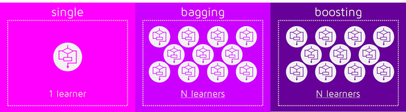
Batch size
- Outside the learning rate, the next important hyperparameter is batch size because it directly impacts on the model’s performance and training time.
- Deep learning models rely on large datasets for achieving high performance. However, when datasets contain millions or even billions of instances, fitting the entire dataset into memory becomes challenging. Additionally, performing a gradient update for each instance would be computationally expensive and time-consuming. To address these issues, batch training is utilized, where the dataset is divided into smaller parts called batches.
- The batch size refers to the number of training instances in each batch. In frameworks like Keras, the batch size is specified using the batch_size argument in the model.fit() method. The acceptable values for the batch size hyperparameter range from 1 to the size of the full training dataset, denoted as “m.” However, there are practical considerations when choosing the batch size.
- Typically, batch sizes that are powers of 2, such as 16, 32, 64, 128, 256, 512, and 1024, are preferred. This is because the batch size needs to fit the memory requirements of the GPU and the architecture of the CPU.
- There are three main variants of gradient descent optimization algorithms based on the batch size:
- Batch Gradient Descent: In this variant, the batch size is set to the size of the full training dataset (m). It involves computing the gradients and updating the model parameters based on the entire dataset. This method can be computationally expensive and memory-intensive but provides a more accurate estimate of the gradients.
- Stochastic Gradient Descent: Here, the batch size is set to 1, meaning that each training instance is considered individually to compute the gradients and update the model parameters. This approach introduces more noise due to the high variance of gradient estimates but allows for faster updates and potentially faster convergence.
- Mini-Batch Gradient Descent: This variant involves setting the batch size to a value greater than 1 and less than m. It strikes a balance between the computational efficiency of batch gradient descent and the faster convergence of stochastic gradient descent. Mini-batch gradient descent processes a subset of instances (a mini-batch) at each iteration.
- When choosing the right batch size, several guidelines can be followed:
- Start with the default batch size of 32 and experiment with other values if needed.
- Begin with smaller batch sizes and gradually increase if necessary.
- Larger batch sizes require more computational resources but converge faster, while smaller batch sizes require fewer resources but may need more epochs to converge.
- Adjust the number of epochs accordingly when using small batch sizes.
- The dataset’s characteristics, network architecture, and optimizer type influence the ideal batch size.
- The learning rate and batch size are often correlated, with larger batch sizes generally benefiting from higher learning rates and vice versa.
- Overall, selecting the appropriate batch size involves considering the trade-off between computational efficiency, training speed, and convergence accuracy, while also taking into account the specific characteristics of the dataset and the model architecture.
- The batch size refers to the number of samples or data points that are processed by the model in each training iteration.
- When training a recommender system, the dataset used for training can be quite large, consisting of millions or even billions of data points. Training on the entire dataset in a single step would be computationally expensive and may not fit into the memory of the training system.
- To overcome this, the data is divided into smaller groups or batches, and the model is trained on each batch sequentially. The batch size determines the number of samples in each batch.
- The choice of batch size can have an impact on the model’s performance and the duration of each training step.
- Larger batch sizes can lead to faster training as more samples are processed in parallel, utilizing the computational resources more efficiently. However, larger batch sizes may also require more memory and can potentially lead to overfitting or convergence issues.
- On the other hand, smaller batch sizes allow for better generalization as the model gets updated more frequently and can adapt to different patterns in the data. However, smaller batch sizes may result in longer training times due to increased overhead in processing smaller batches.
- The appropriate batch size for training a recommender system depends on factors such as the available computational resources, the complexity of the model, and the size of the dataset. It is often determined through experimentation and fine-tuning to find the optimal balance between training speed and model performance.
- The image below (source), displays the batch_size variable in the context of a training config.
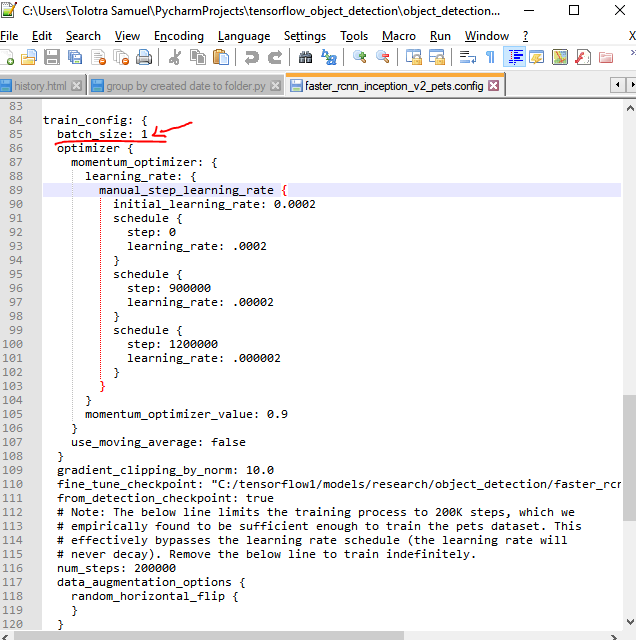
Step or Iteration
- During the training of a model, a training step refers to one gradient update where a certain number of examples, known as the batch size, are processed. The batch size determines how many examples are used to update the gradients of the model in a single step.
- For example, if the batch size is set to 20, it means that during one training step, 20 pictures or rows of data will be processed, and the gradients of the model will be updated based on these 20 examples.
- The duration of a training step is an important metric that is often logged during the training process. It represents the time it takes for the model to process the batch of examples and update the gradients. In the training logs, the step duration is usually displayed in brackets, indicating the time taken per step.
- By adjusting the batch size, it is possible to impact the step duration. Smaller batch sizes tend to result in shorter step durations as fewer examples are processed in each step. For instance, reducing the batch size to 1 (processing one picture per step) can lead to significantly shorter step durations, as shown in the example.
- However, it’s important to note that reducing the batch size does not necessarily reduce the overall training duration. This is because as the batch size decreases, the number of steps required to process the entire dataset increases. So while each step may be faster with a smaller batch size, more steps are needed to complete the training.
-
For instance, if a dataset contains 20,000 pictures and the batch size is set to 1, it would take 20,000 steps to process the entire dataset. On the other hand, if the batch size is increased to 20, it would only require 1,000 steps to process the entire dataset.
- \[Number of steps per EPOCH = Count of training examples / Batch Size\]
- The image below (source), displays a training step as logged by the model in the terminal
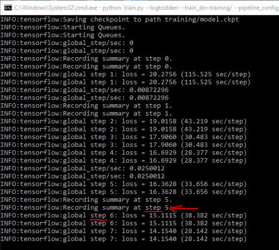
Epoch
- An epoch represents a complete cycle through the entire training dataset. During one epoch, the model processes and learns from all the available training examples.
- The number of epochs required to complete the training depends on various factors and there is no definitive answer. It is determined by the performance of the model and the convergence of the training process. Generally, more epochs can lead to better model performance, as the model has more opportunities to learn and adjust its parameters.
- However, it is important to be cautious of overfitting the model. Overfitting occurs when the model becomes too specialized to the training data and performs poorly on new, unseen data. Training for too many epochs can increase the risk of overfitting. Therefore, it is crucial to monitor the model’s performance on validation data and consider early stopping techniques to prevent overfitting. These techniques involve stopping the training process when the model’s performance on the validation set starts to degrade.
- Ultimately, the number of epochs to use in training is a hyperparameter that needs to be tuned based on experimentation and validation results. It is a balance between allowing the model to learn sufficiently from the data and preventing overfitting.
Loss
- “Loss is the penalty for a bad prediction. That is, loss is a number indicating how bad the model’s prediction was on a single example. If the model’s prediction is perfect, the loss is zero; otherwise, the loss is greater. The goal of training a model is to find a set of weights and biases that have low loss, on average, across all examples.” (source)
- The loss function is a critical metric to monitor during model training as it reflects the model’s performance in making predictions. The goal is to minimize the loss over time, indicating that the model is improving in its predictive capabilities. While occasional spikes in the loss may occur, it is generally expected that the loss should decrease steadily throughout the training process.
- If the loss fails to decrease or shows a consistent upward trend, it is essential to investigate and review the dataset. An increasing loss could indicate issues such as incorrect labeling, data quality problems, or insufficient data representation. By examining the dataset, you can identify potential issues that might be hindering the model’s performance.
- It is crucial to ensure the dataset is properly prepared and representative of the problem you are trying to solve. This includes verifying the correctness of labels, checking for missing or noisy data, and assessing the data distribution. By addressing any dataset-related issues, you can improve the training process and potentially achieve better model performance.
- Regularly monitoring the loss and taking necessary steps to review and refine the dataset will contribute to training a more effective and accurate model.
- The image below (source), shows the loss steadily decreasing and getting closer to convergence.
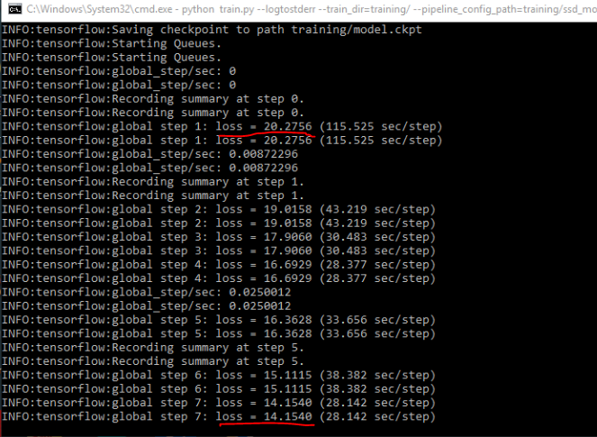
Sparsity
- “In AI inference and machine learning, sparsity refers to a matrix of numbers that includes many zeros or values that will not significantly impact a calculation.”(source)
- Improved model efficiency: Sparsity reduces the number of non-zero elements in the model, leading to more efficient computations and memory usage. By eliminating unnecessary parameters or features, sparse models can be faster and require less storage, making them more practical for deployment on resource-constrained devices or in large-scale systems.
- Feature selection and interpretability: Sparsity can help identify the most relevant features or inputs for a given task. By encouraging sparsity in the model’s weights or feature representation, less important or redundant features can be effectively ignored, leading to a more compact and interpretable model. This can facilitate better understanding and insights into the underlying patterns and relationships in the data.
- Regularization and generalization: Sparsity acts as a form of regularization, preventing overfitting by reducing model complexity. By encouraging sparsity, the model becomes more robust and less prone to fitting noise or irrelevant details in the training data. This regularization effect helps improve generalization, allowing the model to perform better on unseen data.
- Compressed model representation: Sparsity can be leveraged to compress models and reduce storage requirements. Sparse representations enable more efficient model storage and transmission, which is particularly valuable in scenarios where bandwidth or storage capacity is limited, such as mobile applications or distributed systems.
- Energy efficiency: Sparse models can consume less energy during both training and inference. The reduced number of operations required for sparse computations leads to lower power consumption, making sparse models more energy-efficient, especially in resource-constrained environments.
- Link to more information on sparsity on Aman.ai.
Why add sparsity
- Sparse vectors often have a large number of dimensions, and creating a feature cross can further increase the dimensionality. This can lead to a significant increase in model size and memory requirements.
- In high-dimensional sparse vectors, it would be beneficial to promote weights to become exactly zero whenever possible. A weight of zero essentially removes the corresponding feature from the model, resulting in memory savings and potentially reducing noise in the model
How to add Sparsity
- L1 Regularization: L1 regularization, also known as Lasso regularization, can encourage sparsity by adding a penalty term to the model’s loss function. This penalty term is proportional to the absolute values of the model’s weights. By minimizing the combined loss and penalty, L1 regularization tends to shrink less important weights to zero, effectively selecting a subset of features or parameters.
- Group Lasso: Group Lasso extends L1 regularization to encourage sparsity at the group level. It is particularly useful when dealing with structured data, such as images or text, where the features can be organized into groups. Group Lasso promotes sparsity by shrinking entire groups of features together, effectively selecting only a subset of groups.
- Elastic Net Regularization: Elastic Net combines both L1 and L2 regularization. It adds a penalty term that is a linear combination of the L1 and L2 norms of the model’s weights. This allows for both sparsity (through the L1 term) and shrinkage (through the L2 term), providing a balance between feature selection and model stability.
- Dropout: Dropout is a regularization technique commonly used in neural networks. It randomly sets a fraction of the neurons or connections to zero during each training iteration. By doing so, dropout encourages individual neurons to be less reliant on the presence of specific input features, promoting a more robust and sparse representation.
- Pruning: Pruning involves iteratively removing or setting small-weight connections to zero after training a model. It can be applied to various types of models, including neural networks. Pruning techniques identify and eliminate connections or weights that contribute less to the model’s performance, resulting in a sparser and more efficient model.
- Quantization: Quantization reduces the precision of the model’s weights or activations, typically from floating-point to fixed-point representation. This reduction in precision can lead to increased sparsity by setting many of the less significant bits to zero, resulting in a more compact and sparse model representation.
- Keep in mind, an excessively sparse models may sacrifice performance or miss important features.
When to remove Sparsity and how?
- There may be situations where removing sparsity is desired in order to improve model performance or address specific requirements. Here are a few scenarios:
- Dense Representations: Sparse vectors with many dimensions can be computationally expensive and memory-intensive, especially when dealing with large-scale datasets. In some cases, transforming sparse vectors into dense representations can be beneficial for efficient storage and faster computations.
- Dense Neural Networks: Sparsity can pose challenges when training deep neural networks that require dense connections. Some network architectures, such as fully connected layers, may require dense representations to propagate information effectively across all dimensions.
- Domain-specific Considerations: Certain domains or applications may have specific requirements that necessitate dense representations. For example, in computer vision tasks, dense feature maps may be required for precise spatial information or detailed visual analysis.
- To remove sparsity and convert sparse vectors into dense representations, you can employ techniques such as:
- Embeddings: Utilize embedding layers to transform high-dimensional sparse input into lower-dimensional dense representations. These embeddings can capture meaningful relationships between features and provide dense vector outputs.
- Dimensionality Reduction: Apply dimensionality reduction techniques like Principal Component Analysis (PCA) or t-SNE to reduce the dimensionality of sparse vectors while preserving important information. This can result in denser representations with reduced computational complexity.
- Feature Engineering: Identify and engineer new features that capture important patterns or interactions within the data. By combining or transforming sparse features, you can create denser feature representations that capture relevant information for the task at hand.
- It’s important to note that the decision to remove sparsity and the techniques used to achieve it should be based on the specific problem, data characteristics, and performance goals of the model.
Inference
- Inference in a model refers to the process of applying a trained model to make predictions or draw conclusions on new, unseen data. During inference, the model takes input data and produces output predictions based on the patterns it has learned from the training data.
- In the context of machine learning and deep learning models, inference involves feeding new input data into the trained model and obtaining the model’s output or predictions. The model applies its learned weights, biases, and activation functions to transform the input data and produce meaningful results.
- During inference, the model’s parameters are typically fixed, and no further training or adjustment of the model takes place. The goal is to leverage the trained model’s knowledge to make accurate predictions or perform specific tasks on unseen data.
- The inference process can vary depending on the type of model and the specific task it is designed for. It could involve processing individual data instances or batches of data, depending on the requirements and efficiency considerations. The output of inference could be a class label, a probability distribution, a regression value, or any other relevant result based on the specific problem the model is addressing.
- In summary, inference is the stage where a trained model is utilized to make predictions or draw conclusions on new, unseen data based on the knowledge it has gained during the training phase.
Reducing loss
- To reduce loss in a machine learning model, you can consider the following techniques:
- Adjust Learning Rate: The learning rate determines the step size taken during model optimization. A higher learning rate may cause overshooting, while a lower learning rate may result in slow convergence. Experimenting with different learning rates can help find an optimal balance that minimizes the loss.
- Regularization: Regularization techniques like L1 or L2 regularization can help prevent overfitting by adding a penalty term to the loss function. This encourages the model to prioritize simpler and more generalizable solutions.
- Increase Training Data: Providing more diverse and representative training data can improve the model’s ability to generalize and reduce overfitting. Augmenting the existing data or collecting additional samples can help achieve this.
- Feature Engineering: Carefully selecting or engineering relevant features can enhance the model’s performance. Feature scaling, dimensionality reduction, or transforming variables can be effective strategies to improve the model’s ability to learn meaningful patterns.
- Model Architecture: Experimenting with different model architectures, such as adding or removing layers, adjusting the number of units per layer, or exploring different activation functions, can impact the model’s performance. Choosing an architecture that suits the complexity of the problem can help in reducing loss.
- Early Stopping: Monitoring the validation loss during training and stopping the training process when the loss starts to increase can prevent overfitting. This ensures that the model is not trained for too long, leading to better generalization.
- Batch Normalization: Applying batch normalization to the model can help stabilize and accelerate the training process. It normalizes the activations of each layer, making the optimization more effective and reducing the likelihood of getting stuck in suboptimal solutions.
- Gradient Clipping: Limiting the magnitude of gradients during backpropagation can prevent exploding gradients, especially in deep neural networks. This can help stabilize the training process and improve convergence.
References
- Why is it bad idea to initialize all weight to same value?
- Why doesn’t backpropagation work when you initialize the weights the same value?
- What is convergence in k-means?
- Clearly explained: Pearson v/s Spearman Correlation Coefficient
- How to choose between Pearson and Spearman correlation?
- Aman Prabhakar on LinkedIn
- Google Cloud’s MLOps topics
Citation
If you found our work useful, please cite it as:
@article{Chadha2020DistilledInterviewQuestions,
  title   = {Interview Questions},
  author  = {Chadha, Aman and Jain, Vinija},
  journal = {Distilled AI},
  year    = {2020},
  note    = {\url{https://aman.ai}}
}