CS229 • Gaussian Discriminant Analysis

• Generative learning algorithms
• Gaussian discriminant analysis
  • The multivariate Gaussian distribution
  • The Gaussian discriminant analysis (GDA) model
  • Making predictions using GDA
• Visualization of generative vs. discriminative learning algorithms
  • GDA
  • Logistic regression
  • Logistic regression vs. GDA
• Why two separate means, but a single covariance matrix?
• Discussion: GDA and logistic regression
• So when would we prefer one model over another?
  • GDA
  • Logistic regression
  • Practical advice on choosing the right algorithm
• Appendix: How do you figure out if your data is Gaussian?
• Other generative learning algorithms
• Further reading
• Citation

Generative learning algorithms

• We’ve mainly looked at learning algorithms that model \(P(y \mid x ; \theta)\), the conditional distribution of \(y\) given \(x\). For instance, logistic regression modeled \(P(y \mid x ; \theta)\) as \(h_{\theta}(x)=g(\theta^{T} x)\) where \(g(\cdot)\) is the sigmoid function. In this section, we’ll talk about a different type of learning algorithm.
• Let’s use a binary classification problem as the motivation behind our discussion. Consider a classification problem in which we want to learn to distinguish between malignant \((y=1)\) and benign \((y=0)\) tumors.
  • Given a training set, an algorithm like logistic regression, the perceptron algorithm or a generalized linear model initially starts with randomly initialized parameters. Over the course of learning, the algorithm performs gradient descent where the straight line hyperplane (or decision boundary) evolves until you obtain a boundary that separates the positive-negative examples – in this case, the malignant and benign tumors.
  • Then, to classify a new sample as either malignant or benign, it checks on which side of the decision boundary the new sample falls in, and makes its prediction accordingly.
• There’s a different class of algorithms which aren’t trying to maximize the likelihood \(P(y \mid x)\), or looking at both classes and searching for the separation boundary. Instead, these algorithms look at the classes one at a time.
  • First, looking at the malignant tumors, we can learn features of what malignant tumors look like. Then, looking at benign tumors, we can build a separate model of what benign tumors look like.
  • Finally, to classify a new tumor, we can match the new sample against the malignant tumor model and the benign tumor model, to see whether the new tumor looks more like a malignant or benign tumor we had seen in the training set.
• Algorithms that try to learn \(P(y \mid x)\) directly (such as logistic regression), or algorithms that try to learn the mapping from the input space \(\mathcal{X}\) to the labels (such as the perceptron algorithm) are called discriminative learning algorithms.
• In this section, we’ll talk about algorithms that instead try to model \(P(x \mid y)\) (and \(P(y)\)). These algorithms are called generative learning algorithms.
  • For instance, if \(y\) indicates whether an example is a benign tumor \((0)\) or an malignant tumor \((1)\), then \(P(x \mid y=0)\) models the distribution of benign tumors’ features, while \(P(x \mid y=1)\) models the distribution of malignant tumors’ features.
  • The model also learns the class prior \(P(y)\) (or the independent probability on \(y\)). To illustrate the concept of a class prior using a practical example – when a patient walks into a hospital, before the doctor’s even seen them, the odds that their tumor is malignant versus benign is referred to the class prior.
  • Thus, a generative learning algorithm builds a model of features for each of the classes in isolation. At test time, the algorithm evaluates a new sample against each of these models, identifies the model it matches most closely against and returns that as the prediction.

• After modeling \(P(y)\) (called the class priors) and \(P(x \mid y)\), our algorithm can then use Bayes’ rule to derive the posterior distribution on \(y\) given \(x\):

  \[P(y \mid x)=\frac{P(x \mid y) P(y)}{P(x)}\]
  • Here, the denominator is given by \(P(x)=P(x \mid y=1) P(y=1)+P(x \mid y=0) P(y=0)\), which is a function of the quantities \(P(x \mid y)\) and \(P(y)\). Note that both of these quantities are learned as part of the learning process of generative learning algorithms.
• Note that if you are calculating \(P(y \mid x)\) in order to make a prediction, then we don’t actually need to calculate the the probability value in the denominator \(P(x)\) since it is a constant, as \(y\) doesn’t even appear in there. When making predictions with generative learning algorithms, you can thus ignore computing the denominator to save on computation. However, if the end goal is a probability value, then you would need to compute the denominator to be able to normalize the probability in the numerator.

• The above equation represents the underlying framework we’ll use to build generative learning algorithms such as Gaussian discriminant analysis and Naive Bayes.
• Key takeaways
  • Discriminative learning algorithms learn \(P(y \mid x)\), i.e., the distribution of the output given an input. In other words, learn \(h_{\theta}(x)=\{0, 1\}\) directly.
  • Generative learning algorithms learn \(P(x \mid y)\), i.e., the distribution of features given a class, and \(P(y)\) which is called the class prior. In the tumor-identification setting, where a tumor may be malignant or benign, these models learn the features for each case and use them to make a prediction.

Gaussian discriminant analysis

• The first generative learning algorithm that we’ll look at is Gaussian discriminant analysis (GDA), which can be used for continuous-valued features, say, tumor classification.
• In this model, we’ll assume that \(P(x \mid y)\) is distributed according to a multivariate normal distribution. Let’s talk briefly about the properties of multivariate normal distributions before moving on to the GDA model itself.

The multivariate Gaussian distribution

• The multivariate Gaussian distribution (also called the multivariate normal distribution) is the generalization of the Gaussian distribution from a 1-dimensional random variable to an \(n\)-dimensional random variable (or simply, \(n\)-random variable). In other words, rather than a uni-variate random variable, the multivariate Gaussian seeks to model multiple random variables.
• Assume \(X\) is distributed as a multivariate Gaussian, i.e, \(X \in \mathbb{R}^{n}\), parameterized by a mean vector \(\mu \in \mathbb{R}^{n}\) and a covariance matrix \(\Sigma \in \mathbb{R}^{n \times n}\), where \(\Sigma \geq 0\) is symmetric and positive semi-definite. Formally, this can be written as,

• The probability density function (PDF) of \(X\) is given by:

  \[P(X ; \mu, \Sigma)=\frac{1}{(2 \pi)^{n / 2}|\Sigma|^{1 / 2}} \exp \left(-\frac{1}{2}(X-\mu)^{T} \Sigma^{-1}(X-\mu)\right)\]
  • where \(“|\Sigma|”\) denotes the determinant of the matrix \(\Sigma\).

• The expected value of \(X\) is given by \(\mu\):

• The covariance of a vector-valued random variable \(X\) is defined as \(\operatorname{Cov}(X)=\) \(\mathrm{E}\left[(X-\mathrm{E}[X])(X-\mathrm{E}[X])^{T}\right]\). Covariance generalizes the notion of the variance of a real-valued random variable to an \(n\)-dimensional setting. The covariance can also be defined as \(\operatorname{Cov}(X)=\) \(\mathrm{E}\left[XX^{T}\right]-(\mathrm{E}[X])(\mathrm{E}[X])^{T}\). Since \(X\) is distributed as a multivariate Gaussian, \(\operatorname{Cov}(X)=\Sigma\).
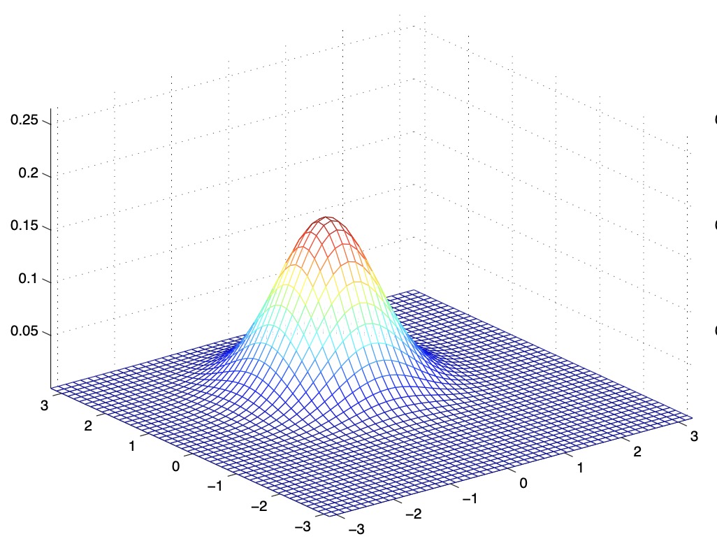
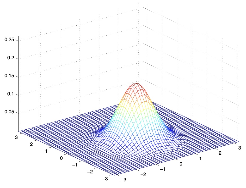
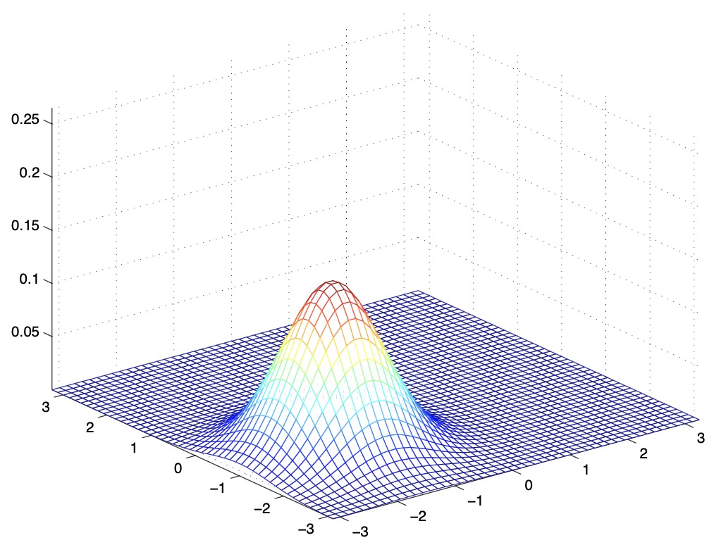
• Let’s explore some examples that visualize the PDF of a Gaussian distribution. Recall that the Gaussian is the familiar bell-shaped curve. Similarly, the multivariable Gaussian is represented by the same bell-shaped curve with two parameters \(\mu\) and \(\sigma\) that control the mean and the variance of the PDF, but in \(n\)-dimensions. For e.g., for a 2-dimensional Gaussian (or a Gaussian over 2 random variables), \(\mu\) is 2-dimensional, while the covariance matrix is of size \(2 \times 2\).
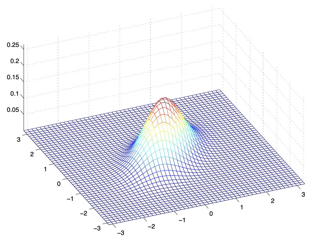
• The below figure shows a Gaussian with zero mean (i.e., the \(2 \times 1\) zero-vector) and covariance matrix \(\Sigma=I\) (the \(2 \times 2\) identity matrix). A Gaussian with zero mean and identity covariance is also called the standard normal distribution.

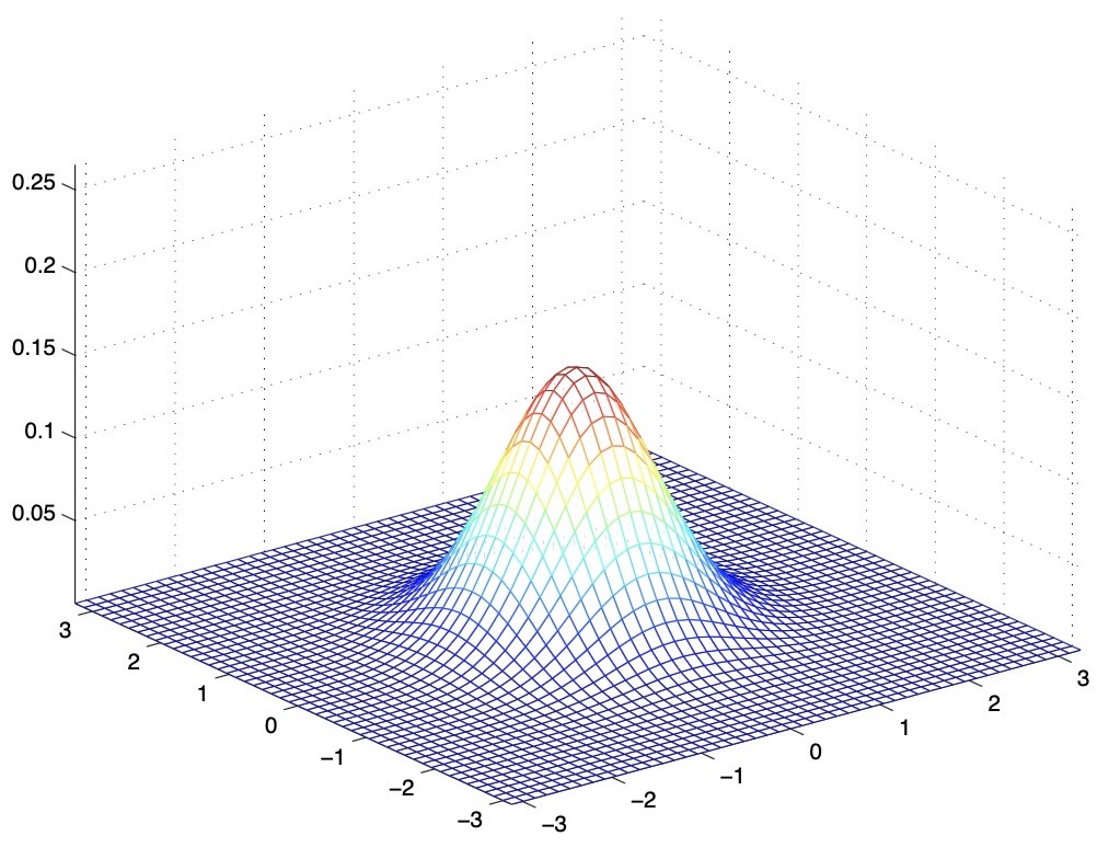
• The figure below shows the PDF of a Gaussian with zero mean and \(\Sigma=0.6 I\). We’ve essentially taken the covariance matrix and multiplied it by a number \(< 1\), which has shrunk the variance, i.e., reduced the variability of our distribution.

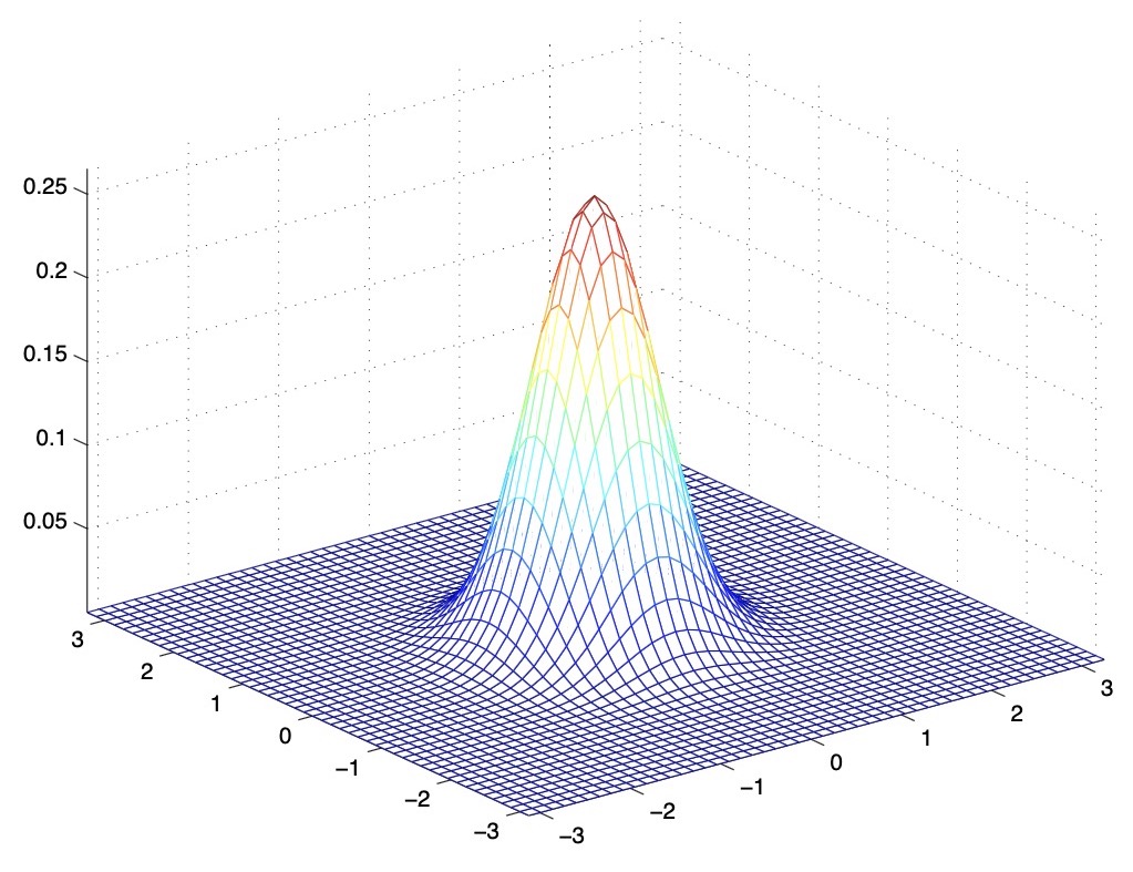
• The figure below shows one with \(\Sigma=2 I\).

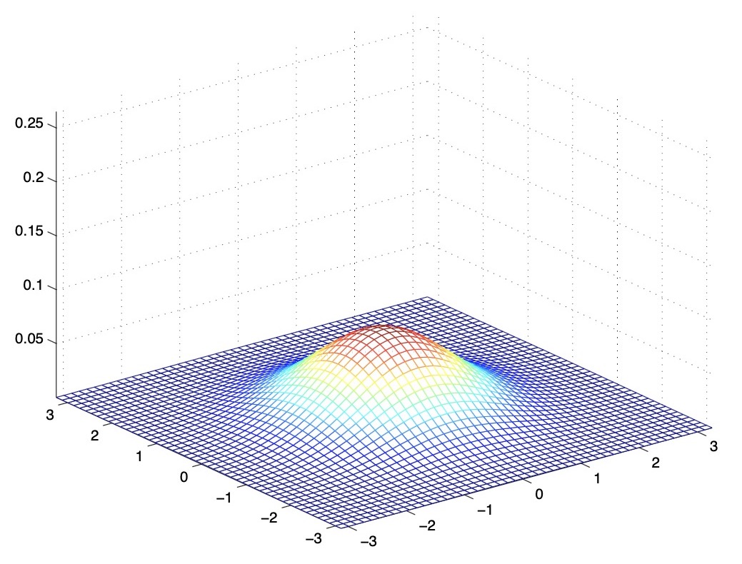
• From the above images, we see that as \(\Sigma\) becomes larger, the Gaussian becomes more “wider/shorter”, and as it becomes smaller, the distribution becomes more “compressed/taller”. This is because the PDF always integrates to 1, i.e., the area under the curve of a PDF function is always 1, so the Gaussian curve scales its spread vs. height accordingly.
• The figures below show Gaussians with mean 0 and their corresponding covariance matrices \(\Sigma\):

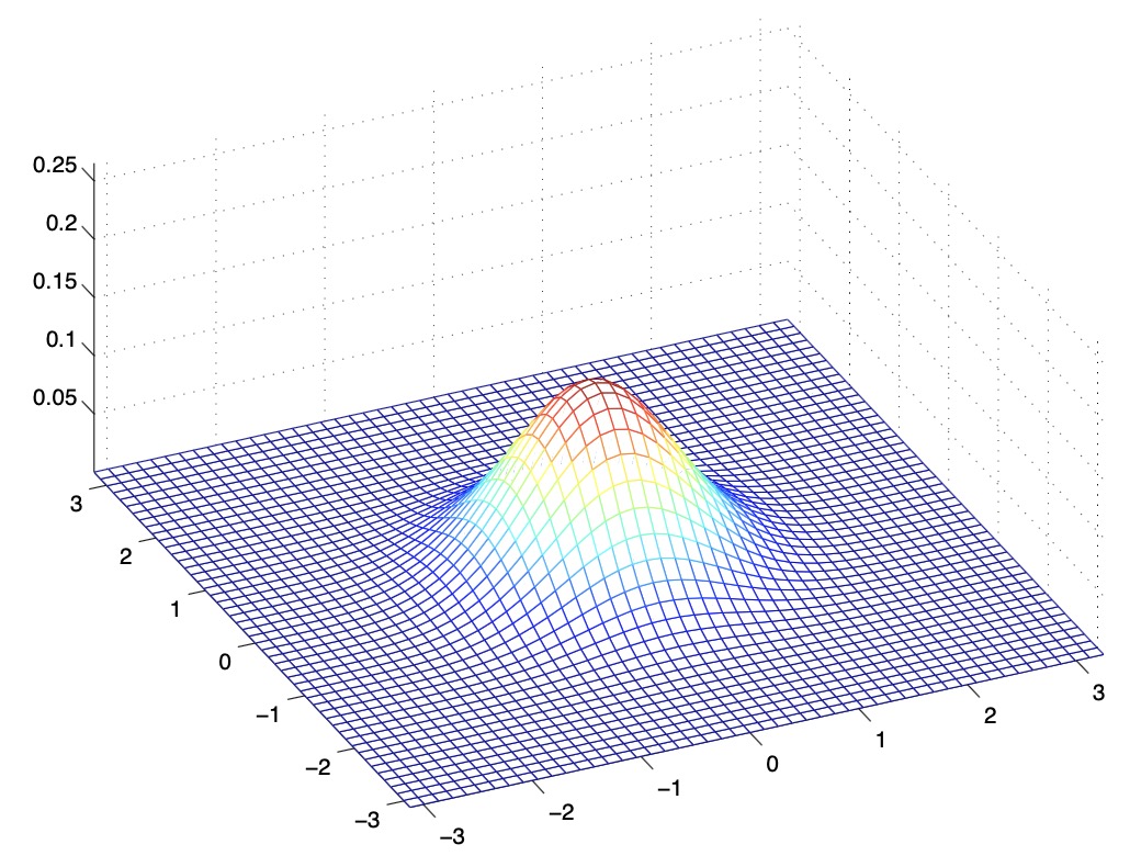
• The figure above shows the standard normal distribution.

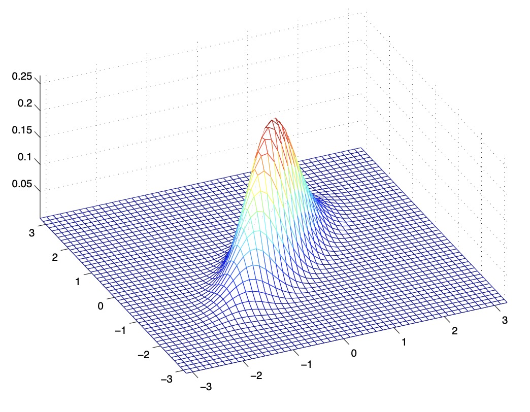
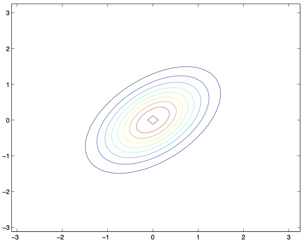
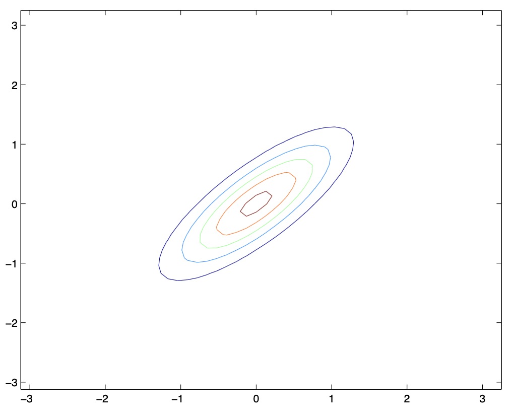
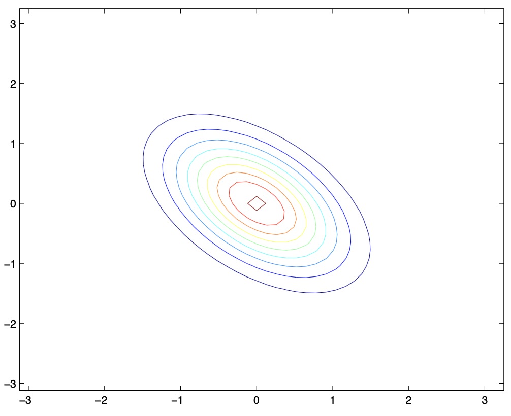
• From the above figures, we see that as we increase the off-diagonal entries in \(\Sigma\), the PDF becomes more “compressed” towards the \(45^{\circ}\) line (given by \(x_{1}=x_{2}\)). Geometrically speaking, this implies that two random variables are positively correlated. We can see this more clearly when we look at the contours of the same three Gaussian densities instead of the 3-D bumps we saw above,

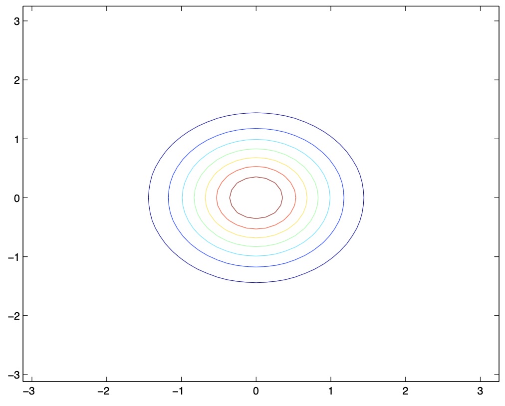
• Note that the above figure should show perfectly round circles, but the aspect ratio of the image probably makes them look a little bit fatter :)

• Thus, as \(\Sigma\) becomes larger, the PDF places value on the random variables being positively correlated.

• Here’s another set of examples along with their corresponding covariance matrices \(\Sigma\):

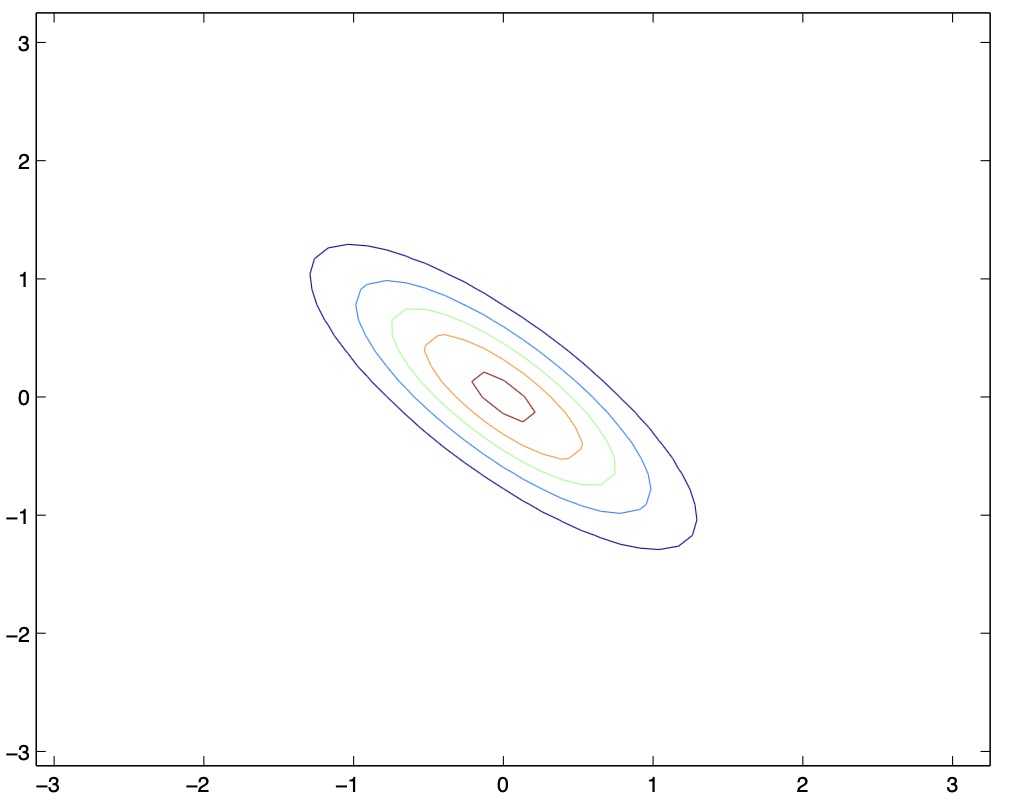
• From the above two figures, we see that by decreasing the off-diagonal elements of the covariance matrix, the PDF now becomes “compressed” again, but in the opposite direction, i.e., towards the \(135^{\circ}\) line. Again, geometrically, you endow the two random variables with negative correlation.

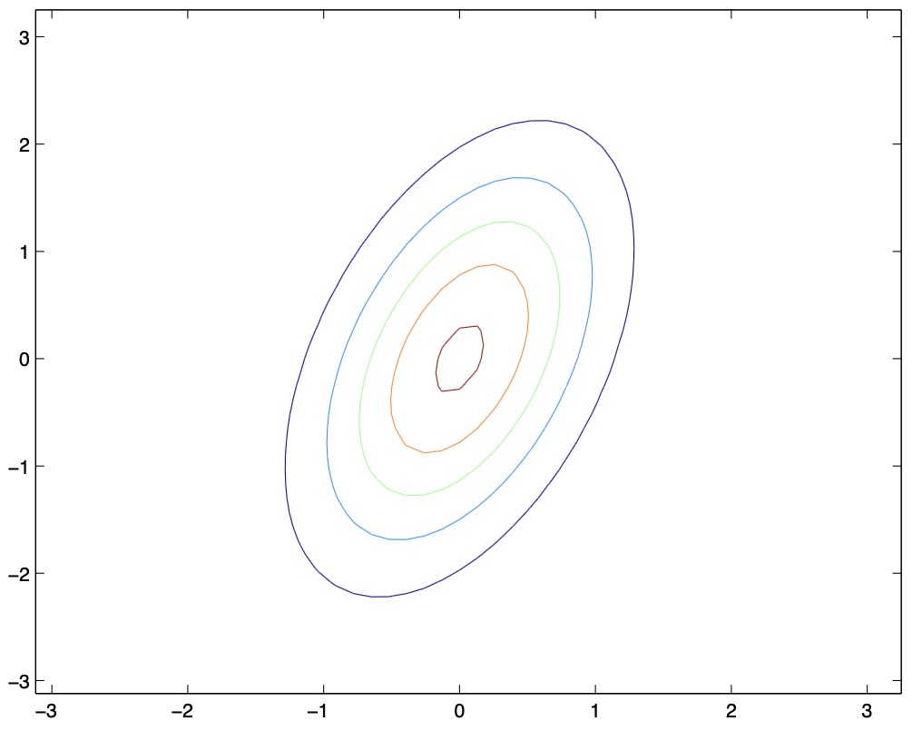
• From the above figures, we see that as we vary the off-diagonal parameters, the contours tend to form ellipses.
• By varying \(\mu\), we can shift the center of the Gaussian density around. Another set of examples with mean values \(\mu\) and \(\Sigma=I\), along with a visualization of their corresponding Gaussian PDFs are as follows:

• Note that if you carry out principal component analysis on the covariance matrix, the eigenvectors points in the principal axes of the ellipse which are defined by the contours.
• Key takeaway
  • As you vary the mean \(\mu\) and the covariance matrix \(\Sigma\) of the Gaussian density, you can change the center and the spread/height of the PDF respectively.

The Gaussian discriminant analysis (GDA) model

• When we have a classification problem in which the input features \(x\) are continuous-valued random variables, we can use the Gaussian Discriminant Analysis (GDA) model, which models \(P(x \mid y)\) using a multivariate normal distribution.
• Let’s consider the tumor-identification task for this discussion, and model it as a Gaussian distribution. This can be expressed using two equations \(P(x \mid y = 0)\) and \(P(x \mid y = 1)\), which essentially model the probability density of the tumor’s features given it is benign or malignant as Gaussians. On the other hand, \(y\) is a Bernoulli random variable, which takes on values \(\{0, 1\}\). Formally, the model is given by,

• Thus, the parameters of our GDA model are \(\mu_0\), \(\mu_1\), \(\Sigma\) and \(\phi\). Note that we used the same covariance matrix \(\Sigma\) for both classes, but different mean vectors \(\mu_0\) and \(\mu_1\). Put simply, we’re assuming that the two Gaussians representing the positive and negative classes have the same covariance matrix but have different means. You can also use different covariance matrices \(\Sigma_0\) and \(\Sigma_1\), but that is not commonly seen. More on this in the section on “why two separate means, but a single covariance matrix?” below.
  • Thus, if you can fit \(\mu_0\), \(\mu_1\), \(\Sigma\) and \(\phi\) to your data, then these parameters will define \(P(x \mid y)\) and \(P(y)\) for your data.
• Note that \(\phi \in \mathbb{R}\), \(\mu_0 \in \mathbb{R}^n\), \(\mu_1 \in \mathbb{R}^n\), and \(\Sigma \in \mathbb{R}^{n \times n}\).
• Writing out the distributions, this is:

• Note that the exponential notation used for \(P(y)\) is similar to what we saw earlier with logistic regression.
• Plugging in the above quantities \(P(x \mid y=0), P(x \mid y=1), P(y=0)\) and \(P(y=1)\) in Bayes’ formula that we saw in the section on generative learning algorithms, you can easily ascertain a tumor as benign or malignant for our particular example.
• Suppose you have a training set, \(\{(x^{(i)}, y^{(i)})\}_{i=1}^m\). To fit the aforementioned parameters to our training set, we’re going to maximize our joint likelihood \(L(\cdot)\),

• The big difference between the cost functions of a generative learning algorithm compared to a discriminative learning algorithm is that in case of a generative learning algorithm like GDA, you are trying to choose parameters \(\phi, \mu_{0}, \mu_{1}, \Sigma\), that maximize the joint likelihood \(P(x, y; \phi, \mu_{0}, \mu_{1}, \Sigma)\). On the other hand, for discriminative learning algorithms such as linear regression, logistic regression or generalized linear models, you are trying to choose parameters \(\theta\), that maximize the conditional likelihood \(P(y \mid x; \theta)\).
• The log-likelihood of the data \(\ell(\cdot)\) is simply the log of the likelihood \(L(\cdot)\). Formally,

• To maximize \(\ell(\cdot)\) with respect to the parameters, we take the derivative of \(\ell(\cdot)\), set the derivative equal to 0 and then solve for the values of the parameters that maximize the expression for \(\ell(\cdot)\). This yields the maximum likelihood estimate of \(\phi\) to be,

• An intuitive explanation around the value of \(\phi\) that maximizes the expression is as follows. Recall that \(\phi\) is the estimate of probability of \(y\) being equal to 1. In our particular example, the chance that the next patient walks into your doctor’s office with a malignant tumor is denoted by \(\phi\). The maximum likelihood of the bias of a coin toss is the fraction of the heads seen. Likewise, the maximum likelihood estimate for \(\phi\) is just the fraction of your training examples with label \(y = 1\).

• Another way to write the above expression for \(\phi\) is using the indicator notation, as follows:

  \[\phi =\frac{\sum_{i=1}^{m} \mathbb{1}\left\{y^{(i)}=1\right\}}{m} \\\]
  • Note that the indicator notation \(\mathbb{1}\{\cdot\}\) represents a function which returns 1 if its argument is true, otherwise 0. In other words, the indicator of a true statement is equal to 1 while that of a false statement is equal to 0. The indicator notation thus represents the equivalent of the if-statement in a programming context.
• The maximum likelihood estimate of the mean vectors \(\mu_0, \mu_1\) is,

• To build intuition around the value of \(\mu_0\) and \(\mu_1\) that maximizes the expression, think about what would be the maximum likelihood estimate of the mean of all of the features for a particular class, say benign tumors, denoted by the class label 0 in our dataset.
• Let’s consider \(\mu_0\). A reasonable way to estimate \(\mu_0\) would be to take all the benign tumors in your training set (all the negative examples, i.e., entries as 0s) and just take the average of their features. The above equation is a way of writing out that intuition. The numerator is the sum of feature vectors for all the examples of benign tumors in the training set (i.e., examples with \(y = 0\)) while the denominator is simply the number of benign tumors in the training set.
  • The numerator sums over the entire set of training examples, i.e., by summing over \(i = 1 \ldots m\), and uses the indicator function to look for instances where \(y_i = 0\) times \(x_i\). The effect of that is that for a benign tumor, this term yields 1 times the features, whereas for a malignant tumor, this yields 0 times the features (effectively zeroing out the term). In other words, the numerator is simply summing up all the feature vectors for all of the benign samples in the training set.
  • On the other hand, the denominator sums over the entire set of training examples, i.e., by summing over \(i = 1 \ldots m\), and uses the indicator function to look for instances where \(y_i = 0\). In other words, the denominator will count up the number of examples that represent benign tumors. Because for every \(y_i = 0\), you get an extra 1 in this sum, the denominator ends up being the total number of benign tumors in your training set.
  • Thus, the ratio represents the mean of the feature vectors of all of the benign examples.
  • A similar argument can be made for \(\mu_1\).
• The maximum likelihood estimate of the covariance matrix \(\Sigma\) is,

• The covariance matrix fits contours of the Gaussian distributions for each of the classes with their corresponding means \(\mu_0, \mu_1\) but you want one covariance matrix for both of the classes.

Making predictions using GDA

• Recall that \(\operatorname{min}_z\) (referred to as \(min\) over \(z\)) returns the minimum value of the expression for any possible value of \(z\). On the other hand, \(\operatorname{argmin}_z\) (referred to as \(argmin\) over \(z\)) refers to the value of \(z\) which when plugged in, yields the minimum value of the expression. For example,
  • \(\operatorname*{min}_{z} (z - 5)^2\) refers to the minimum value attained by the expression \((z - 5)^2 = 0\) for any \(z\).
  • \(\operatorname*{argmin}_{z} (z - 5)^2\) refers to the value of \(z\) that led to the minimum value of the expression \((z - 5)^2\), which in this case would be \(z = 5\).
• Similarly, the \(\operatorname{max}_z\) and \(\operatorname{argmax}_z\) operators also exist and they deal with the maximum value of the expression and the value of the \(z\) that leads to the maximum value of the expression respectively.

• Finally, having fit these parameters, let’s figure out how we may go about making a prediction. So given a new tumor, how do you make a prediction for whether it is malignant or benign? The problem boils down to predicting the most likely class label \(y\) given an input sample \(x\), which can be formally written as:

  \[\operatorname*{argmax} _{y} P(y \mid x)\]
  • Looking deeper into the equation above, we’re essentially looking to choose a value of \(y = \{0, 1\}\) that maximizes the above expression.

• Using Bayes’ rule,

  \[\operatorname*{argmax} _{y} P(y \mid x) = \operatorname*{argmax} _{y} \frac{P(x \mid y) P(y)}{P(x)}\]
  • We do not need to calculate \(P(x)\) in the denominator for the same reasons highlighted in the section on Generative Learning Algorithms.

Visualization of generative vs. discriminative learning algorithms

• Let’s look at a dataset and compare-and-contrast how a generative (GDA) vs. discriminative (logistic regression) learning algorithm would operate on the dataset.

GDA

• Pictorially, GDA’s operation can be seen as follows:

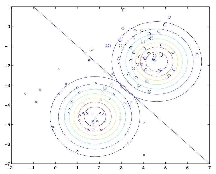
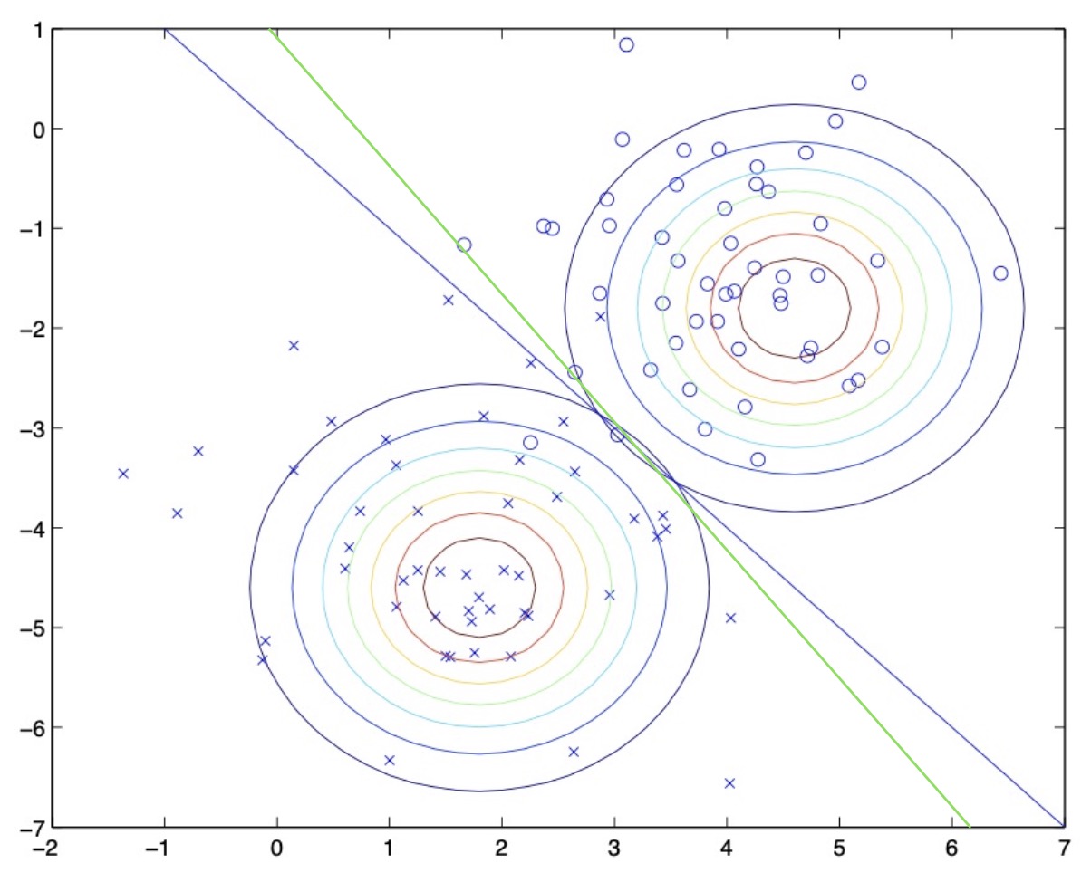
• Shown in the figure is the training set, as well as the contours of the two Gaussian distributions that have been fit to the data in positive and negative examples. Note that the two Gaussians have contours that are the same shape and orientation, since they share a covariance matrix \(\Sigma\), but they have different means \(\mu_{0}\) and \(\mu_{1}\).
• For each point, we determine the class label using Bayes’ rule, and put together, they imply the decision boundary (in blue) in the figure above, at which \(P(y=1 \mid x)=0.5\). On one side of the boundary, we predict \(y=1\) to be the most likely outcome, and on the other side, we predict \(y=0\). Points to the upper right of this decision boundary are closer to the negative class, and you thus end up classifying them as negative examples and points to the lower left of the decision boundary are classified as positive examples.

Logistic regression

• The figure below shows an example with two features \(x_1\) and \(x_2\) and positive and negative examples. Let’s start with a discriminative learning algorithm such as logistic regression whose parameters have been initialized randomly.

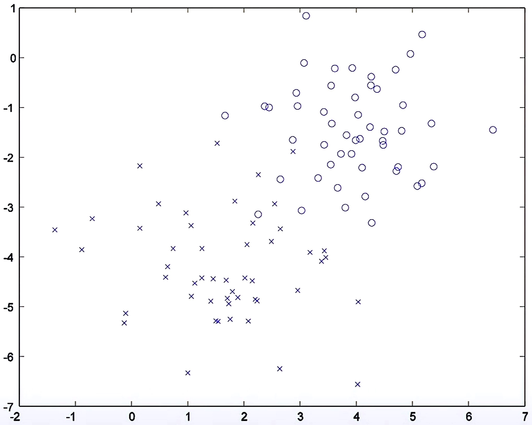
• Typically, when you carry out logistic regression, you initialize the parameters as zero but for the purpose of this visualization, we’re starting off with a random decision boundary as shown below.

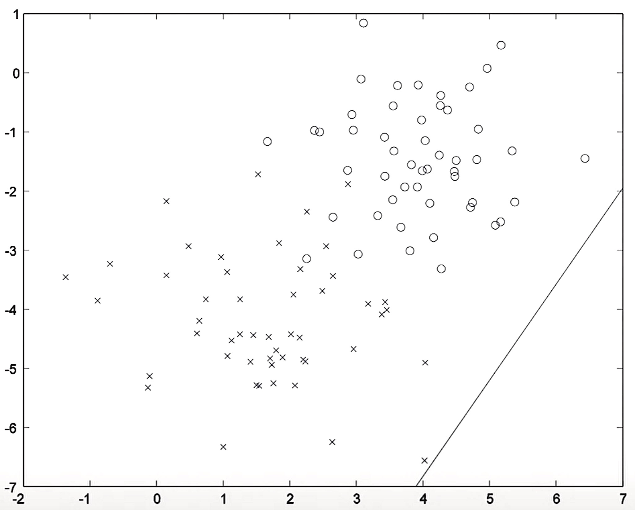
• Running a single iteration of gradient descent on the conditional likelihood \(P(Y \mid X)\), one iteration of logistic regression re-positions the decision boundary:

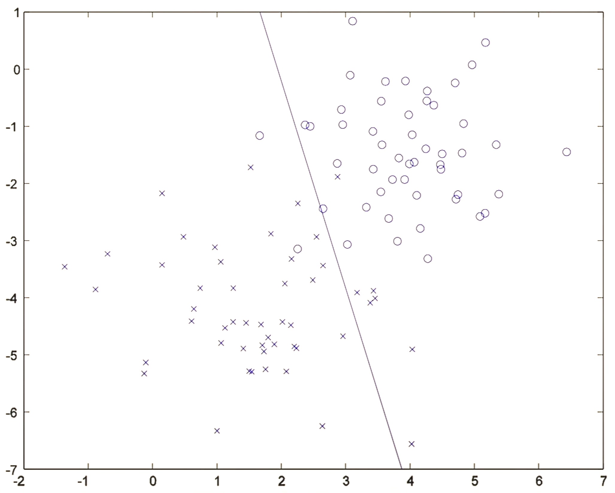
• After about 20 iterations, the algorithm converges to a discriminative boundary as shown below:

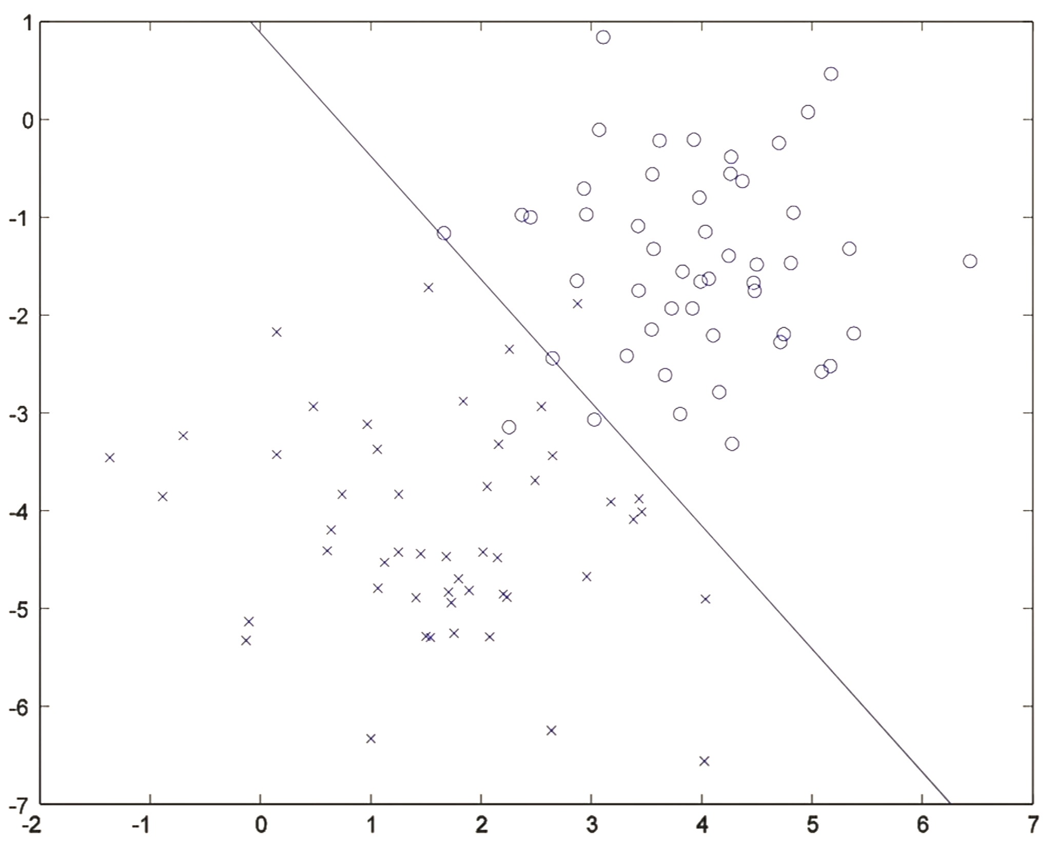
• Logistic regression is thus essentially searching for a line (also called a decision boundary) that separates positive and negative examples.

Logistic regression vs. GDA

• The figure below illustrates the decision boundary for logistic regression (in green) superimposed on the figure above (where the decision boundary for GDA is shown in blue). Note that the two algorithms actually arrive at slightly different decision boundaries.

Why two separate means, but a single covariance matrix?

• If you choose to build a model using two separate means and a single covariance matrix, the decision boundary ends up being linear which is the case for a lot of problems.
• Choosing to use two separate covariance matrices \(\Sigma_0\) and \(\Sigma_1\) is reasonable, and should work just fine. The catch, though, is that you’ll roughly double the number of parameters and you end up with a decision boundary that isn’t linear anymore.

Discussion: GDA and logistic regression

• Comparing GDA to logistic regression, we see that both share an interesting relationship. Let’s say you’ve learned a set of parameters \(\phi, \mu_{0}, \mu_{1}, \Sigma\). For a fixed value of \(x\), you can compute \(P(y=1 \mid x ; \phi, \mu_{0}, \mu_{1}, \Sigma)\). Using Bayes’ theorem,

  \[P(x \mid y=1 ; \phi, \mu_{0}, \mu_{1}, \Sigma) = \frac{P(x \mid y=1 ; \phi, \mu_{0}, \mu_{1}, \Sigma) P(y=1; \phi)}{P(x; \phi, \mu_{0}, \mu_{1}, \Sigma)} \tag{1}\]
  • where,
    • \(P(x \mid y=1 ; \phi, \mu_{0}, \mu_{1}, \Sigma)\) is a probability measure that you compute by evaluating the Gaussian PDF once you have determined the optimum value of all the parameters.
    • \(P(y=1; \phi)\) is the Bernoulli probability, which can simply be written as \(\phi\).

• Let’s plot the function for \(P(y = 1 \mid x)\) for different values of \(x\). To do so, let’s consider a simple dataset with a single feature \(x\) and a few negative examples and a few positive examples, as shown below:

• Now, let’s see how GDA would operate on this dataset. Mapping/projecting our dataset on to the X-axis,

• Let’s fit a Gaussian to each of the two classes. The bump on the left is \(P(X \mid Y = 0)\) while that on the right is \(P(X \mid Y = 1)\). We’re thus modeling the Gaussian densities of class 0 and class 1. Also, note that we set the same variance to the two Gaussians.
• Because the dataset is split 50-50 across the two classes, \(P(Y = 1)\) is 0.5, which is also known as the one half prior.
• Next, let’s plot \(P(Y = 1 \mid X)\) for different values of \(X\).

• Consider an unlabeled example far to the left on the X-axis. Using equation \((1)\), we can infer that the point almost certainly came from the Gaussian on the left, representing class 0. Because the chance of the class 1 Gaussian generating an example all the way to left of the X-axis is almost 0. In other words, the chance of \(P(Y = 1 \mid X)\) for such a datapoint is very small.
• Let’s pick another point at the center of the X-axis. It’s not easy to discern if this example came from the Gaussian corresponding to the negative or the positive class, which implies that the probability of this example is split 50-50 between the negative or the positive class, i.e., \(P(X \mid Y = 1) = 0.5\).
• Similarly, if you consider a point all the way to the right, you’d be pretty sure this came from the the Gaussian corresponding to the positive class.
• If you repeat the above exercise sweeping datapoints on a dense grid from left to right on the X-axis and evaluate the formula denoted by equation \((1)\), you will get a probability measure, which is essentially a number between 0 and 1. You’ll notice that for points far to the left, the chance of them coming from the positive class \(P(Y = 1)\) is very small. As you approach the midpoint, this chance increases to 0.5 and then surpasses 0.5. Beyond a certain point, it tends to 1. Plotting \(P(Y = 1 \mid X)\) for different values of \(X\) yields a curve like the one below:

• Note that if you connect the dots, then the shape of the curve turns out to be exactly a sigmoid function.

• Thus, if we view the quantity \(P(y=1 \mid x ; \phi, \mu_{0}, \mu_{1}, \Sigma)\) as a function of \(x\), we’ll find that it can be expressed in the form,

  \[P(y=1 \mid x ; \phi, \Sigma, \mu_{0}, \mu_{1})=\frac{1}{1+\exp (-\theta^{T} x)}\]
  • where \(\theta\) is some appropriate function of \(\phi, \Sigma, \mu_{0}, \mu_{1}\). Note that this uses the convention of redefining the \(x^{(i)}\)’s on the right-hand-side to be \(n+1\) dimensional vectors by adding the extra coordinate \(x_{0}^{(i)}=1\). This is exactly the form that logistic regression – a discriminative algorithm – used to model \(P(y=\) \(1 \mid x)\).
• Key takeaways
  • While logistic regression directly uses the sigmoid function as its hypothesis function, under the hood GDA also ends up using the sigmoid function to calculate \(P(Y = 1 \mid X)\) using equation \((1)\).
  • The specific choice of the parameters discriminative learning algorithms like logistic regression and generative learning algorithms like GDA end up choosing can be quite different leading to two different decision boundaries.

So when would we prefer one model over another?

• In general, GDA and logistic regression yield different decision boundaries when trained on the same dataset as seen in the section on “Logistic Regression vs. GDA”. Which is better? In this section, we’ll discuss when a generative algorithm like GDA is superior compared to a distributed algorithm like logistic regression and vice-versa.

GDA

• Formally, GDA assumes that,

  \[\begin{aligned} x \mid y=0 & \sim \mathcal{N}\left(\mu_{0}, \Sigma\right) \\ x \mid y=1 & \sim \mathcal{N}\left(\mu_{1}, \Sigma\right) \\ y & \sim \operatorname{Bernoulli}(\phi) \end{aligned} \tag{2}\]
  • where,
    • \(x \mid y=0\) is Gaussian with mean \(\mu_0\) and covariance \(\Sigma\).
    • \(x \mid y=1\) is Gaussian with mean \(\mu_1\) and covariance \(\Sigma\).
    • \(y\) is Bernoulli with parameter \(\phi\).

• On the other hand, logistic regression assumes that \(P(y = 1 \mid x)\) is logistic, which implies that it is governed by the logistic function,

  \[P(y = 1 \mid x) = \frac{1}{1+\exp (-\theta^{T} x)} \tag{3}\]
  • where,
    • The first element of \(x\), denoted by \(x_0\), is 1.
• The argument that we raised in the above section on “Discussion: GDA and Logistic Regression” by plotting \(P(y = 1 \mid x)\) point-by-point which ultimately yielded the sigmoid curve, illustrates that if \(P(x \mid y)\) is multivariate Gaussian (with shared \(\Sigma\)), then \(P(y \mid x)\) necessarily follows a logistic function. In other words, the set of assumptions given by equations \((2)\) implies that \(P(y = 1 \mid x)\) is governed by the logistic function, i.e., equation \((3)\).
  • However, the converse, i.e., the implication in the opposite direction, is not true, i.e., \(P(y \mid x)\) being a logistic function does not imply \(P(x \mid y)\) is multivariate Gaussian. In other words, assuming equation \((3)\) does not in any way shape or form assume equations \((2)\).
• This shows that GDA makes stronger modeling assumptions about the data than logistic regression (because you can prove the assumptions in equation \((3)\) from the assumptions in equations \((2)\)), which can be noted as an interesting property of GDA.
  • Thus, when your modeling assumptions are correct, GDA will find better fits to the data, and is a better choice for a model than logistic regression. Specifically, when \(P(x \mid y)\) is indeed Gaussian (with shared \(\Sigma\)), GDA is asymptotically efficient.

In general, what you see in a lot of learning algorithms is that if you make strong modeling assumptions about your data and if your modeling assumptions are roughly correct, then your model will do better because you’re baking in more information for the algorithm, along with the dataset itself.

• Informally, this means that in the limit of very large training sets (large \(m\)), there is no algorithm that is strictly better than GDA (in terms of, say, how accurately they estimate \(P(y \mid x)\)).
  • In particular, it can be shown that in this setting, GDA will be a better algorithm than logistic regression; and more generally, even for small training set sizes, we would generally expect GDA to better.

However, the flipside with GDA is that if the assumptions in equations \((2)\) turn out to be incorrect, i.e., if \(x \mid y\) is not Gaussian, then you might be trying to fit a Gaussian density to data that is not inherently Gaussian which would lead to GDA doing poorly. In such cases, logistic regression would be a better choice.

• Note that using two separate covariance matrices \(\Sigma_0\) and \(\Sigma_1\) still leads to a logistic function but with a bunch of quadratic terms in the function. This eventually leads to a non-linear decision boundary, such as one with the positive and negative examples separated by a circular decision boundary.

Logistic regression

• Consider the following assumptions,

  \[\begin{aligned} x \mid y=0 & \sim \operatorname{Poisson}(\lambda_{0}) \\ x \mid y=1 & \sim \operatorname{Poisson}(\lambda_{1}) \\ y & \sim \operatorname{Bernoulli}(\phi) \end{aligned}\]
  • where,
    • \(x \mid y=0\) is Poisson with mean \(\lambda_0\).
    • \(x \mid y=1\) is Poisson with mean \(\lambda_1\).
    • \(y\) is Bernoulli with parameter \(\phi\).
• The above assumptions, if true, imply that \(P(y \mid x)\) follows a logistic function. Logistic regression will thus work well on Poisson data distributions like the ones above. On the other hand, GDA would not and we saw why in the section on GDA above.
• Further, there are many different sets of assumptions that would lead to \(P(y \mid x)\) taking the form of a logistic function. In general, these assumptions apply for any generalized linear model, where the two distributions vary only according to the natural parameter of the exponential family distribution. This implies that if you do not know whether your data is Gaussian or Poisson (and thus aren’t able to make assumptions about the underlying data distribution), logistic regression would still serve well in any case.
  • But if we were to use GDA on such data – and fit Gaussian distributions to non-Gaussian data (like the one above, which follows a Poisson distribution) – then the results will be less predictable, and GDA may not do well.
• Thus, in contrast to GDA, logistic regression is more robust and less sensitive to incorrect modeling assumptions since it makes significantly weaker assumptions.
• Key takeaways
  • Compared to say logistic regression for classification, GDA is simpler and more computationally efficient to implement in some cases. In case of small data sets, GDA might be the better choice than logistic regression.
  • GDA makes stronger modeling assumptions, and is more data efficient (i.e., requires less training data to learn “well”) when the modeling assumptions are correct or at least approximately correct. Thus, if you have a very small dataset, using a model that makes more assumptions will actually allow you to do better because by making more assumptions you’re baking in more information to the algorithm about the dataset (in this case, telling it that the dataset is Gaussian). If the dataset is indeed Gaussian, then the algorithm will actually do better.
  • On the flip side, Logistic regression makes weaker assumptions, and is significantly more robust to deviations in modeling assumptions (such as accidentally assuming the data is Gaussian when it is not). Thus, if you’re trying to fit a binary classification model to a dataset, and if you do not know the underlying nature of the distribution (Gaussian/Poisson/some other member of the exponential family), logistic regression will do fine under any scenario because it does not make assumptions about the distribution of the underlying data. Specifically, when the data is indeed non-Gaussian (say Poisson), then in the limit of large datasets, logistic regression will almost always do better than GDA. For this reason, logistic regression is used more often than GDA in practice.

Practical advice on choosing the right algorithm

• How do you actually choose which algorithm to use?
• The algorithm has two sources of knowledge:
  • The assumptions about the data that you pass on the algorithm.
  • The data itself.
• In today’s era of big data, there is a strong trend to use logistic regression which makes less assumptions about the data and just lets the algorithm figure out whatever it wants to figure out from the data. Thus, for problems that have a lot of data available, logistic regression should be the algorithm of choice. Because with more data, you could overcome telling the algorithm less about the nature of the data.
• On the flip side, the choice of a generative algorithm like GDA over a discriminative algorithm like logistic regression is motivated more by computation and less by performance. In other words, a practical reason behind choosing GDA is that it is computationally efficient. In cases where you’re looking to fit a ton of models and don’t have the time and computational resources to run logistic regression iteratively, GDA is the better option since computing mean and covariance matrices is very efficient.
• Note that the flip-side (as we highlighted in the earlier section) is indeed the fact that the assumptions made are much more stronger, which can affect performance of the model negatively if the dataset doesn’t agree with those assumptions, causing a hit in model accuracy.
• The question of whether you make strong or weak assumptions is actually a general philosophical point. This is a general principle in machine learning that we see in a lot of learning algorithms.
• A lot of the skill in machine learning these days is getting your algorithms to work even when you don’t have millions of examples which is typically the case. There are lots of machine learning applications where you have a hundred examples and it’s the skill in designing your learning algorithms that matters much more.
• Consider ImageNet, which has over a million images. There are typically dozens of teams that can get great results. Owing to the large dataset, the performance difference between teams is relatively minimal. But if you only have a hundred examples, then the high-skilled teams will actually do much better than the low skilled teams, whereas the performance gap is smaller when you have giant datasets.
• Thus, when working with a limited dataset, your intuitions should fuel your assumptions – for e.g., whether you use a generative or discriminative algorithm. These intuitions distinguish the high-skilled teams from the less experienced teams and drive a lot of the performance differences when you have a small dataset.
  • There are a lot of applications where your skill at designing a machine learning system really makes a big difference especially when you have a limited dataset. When you don’t have much data, the assumptions that you bake into your model such as whether your dataset is Gaussian or Poisson allow you to drive much bigger performance gains than a less experienced team would be able to.

Appendix: How do you figure out if your data is Gaussian?

• Most data in this universe is Gaussian – it’s actually a matter of degree. Particularly, most error/noise distributions can be modeled as Gaussian distributions.
• If a distribution is made up of several noise sources which are not too correlated, then we can assume it be a Gaussian using the central limit theorem from statistics.
• Plotting a given dataset offers insight into whether the data is Gaussian or not. Most data will not fully be Gaussian but can be vaguely Gaussian – it just depends on the amount of degree.

Other generative learning algorithms

• Some related considerations about discriminative vs. generative models also apply to the Naive Bayes algorithm, but the Naive Bayes algorithm is still considered an effective and popular classification algorithm.

Further reading

Here are some (optional) links you may find interesting for further reading:

• Learning in graphical models by Michael I. Jordan and Generalized Linear Models 2nd ed. by McCullagh and Nelder served as a major inspiration for our discussion on this topic.

Citation

If you found our work useful, please cite it as:

@article{Chadha2020DistilledGaussianDiscriminantAnalysis,
  title   = {Gaussian Discriminant Analysis},
  author  = {Chadha, Aman},
  journal = {Distilled Notes for Stanford CS229: Machine Learning},
  year    = {2020},
  note    = {\url{https://aman.ai}}
}