CS229 • Perceptron
The perceptron algorithm
- The perceptron algorithm was invented in 1958 at the Cornell Aeronautical Laboratory by Frank Rosenblatt. It was argued to be an approximate model for how individual neurons in the brain work. Given how simple the algorithm is, it will also provide a starting point for our analysis during our discussion on the topic of learning theory.
- The perceptron algorithm can be viewed as a simplified variant of the logistic regression algorithm. Consider modifying the logistic regression method to “force” it to output values that are either 0 or 1, i.e., \(\{0, 1\}\). To do so, it seems natural to change the definition of \(g(\cdot)\) to the step/threshold function:
-
Using the same update rule as logistic regression, but using the above (modified) definition of \(g(\theta^{T} x)\) as \(h_{\theta}(x)\), yields the perceptron learning algorithm.
\[\theta_{j}:=\theta_{j}+\alpha\left(y^{(i)}-h_{\theta}(x^{(i)})\right) x_{j}^{(i)} \tag{1}\]- where,
- \(\alpha\) is the learning rate (i.e., the step size).
- \(x_{j}^{(i)}\) represents the the \(j^{th}\) feature of the \(i^{th}\) training sample.
- where,
- Note that the update rules for the perceptron, logistic regression and linear regression are all similar, with the only difference being the definition of \(h_{\theta}(x)\) or \(g(\theta^{T} x)\). The reason behind this common theme is that these algorithms are types of generalized linear models.
- Even though the perceptron may be cosmetically similar to the other algorithms, it is actually a very different type of algorithm than logistic regression and least squares linear regression; in particular, it is difficult to endow the perceptron’s predictions with meaningful probabilistic interpretations (unlike logistic regression), or derive the perceptron as a maximum likelihood estimation algorithm. As such, the perceptron algorithm is not something that is widely used in practice, and is mostly of historical interest.
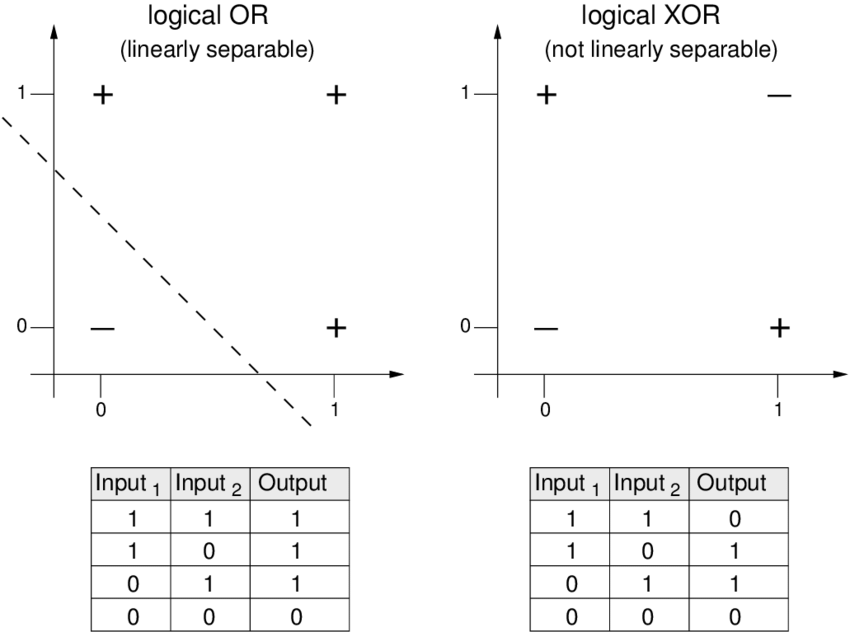
- In 1969, a famous book entitled Perceptrons by Marvin Minsky and Seymour Papert showed that it was impossible for a single layer perceptron to learn a function that is not linearly separable, such as the XOR function (cf. figure below). Thus, single layer perceptron perceptons have limited use, and can be applied to correctly classify only linearly separable functions such as the OR function (cf. figure below). However, note that multi-layer perceptrons are capable of producing an XOR function.
Example
- Let’s consider an example to understand the process of learning with the perceptron and its limitations. The following graph shows the input space with two classes, squares and circles. Your goal is to learn an algorithm that can separate the two classes.

- The algorithm learns one example at a time in an online manner. Let’s assume that the algorithm has thus far, learned \(\theta\) that represents the hyperplane/decision boundary \(d_1 = \theta^T x = 0\) shown in the graph above with a dotted line. Note that,
- Anything upwards the decision boundary is given by \(\theta^T x > 0\) and,
- Anything below the decision boundary is given by \(\theta^T x < 0\).
- When a new example \(x^{(i)}\) comes in, say a square, the algorithm will misclassify it based on our initial decision boundary \(d_1\).

- Now, the vector representation of our initial decision boundary \(d_1\) would be a vector \(\theta\) that’s normal to the line. We’ve also shown the vector representation of our new example \(x\), which got misclassified.
- Inspecting the update rule in equation \((1)\) above, we notice that the quantity \(\left(y^{(i)}-h_{\theta}(x^{(i)})\right)\) is a scalar (since we’re only considering a single training example \((x^{(i)}, y^{(i)})\) for now). This quantity can either be:
- 0 if the algorithm got its prediction right or,
- \(+1\) if the algorithm got its prediction wrong and \(y^{(i)} = 1\) or,
- \(-1\) if the algorithm got its prediction wrong and \(y^{(i)} = 0\).
- Assuming the square class to be our positive class (denoted by 1) and the circle class to be our negative class (denoted by 0), our new example \(x^{(i)}\) would be misclassified as a 0 even though its a 1.
- Thus, the quantity \(\left(y^{(i)}-h_{\theta}(x^{(i)})\right)\) in the update rule would be \(1-0 = 1\).
- Next, the algorithm uses the update rule to update \(\theta\):
- The updated value of \(\theta\), denoted by \(\theta’\), leads to the new decision boundary \(d_2\), as shown in the below diagram. Note that with \(d_2\), \(x^{(i)}\) is now included in the positive class.

- Thus, since the example was misclassified, you either add a small component of the example itself \(\alpha x_{j}^{(i)}\) to \(\theta\) or you subtract it, depending on the class of the example. Now, had the new example \(x^{(i)}\) been correctly classified, the algorithm doesn’t make any changes to its decision boundary.
- Key takeaways
- The perceptron goes example by example in an online manner, and alters \(\theta\) depending on whether it was able to classify the incoming example \(x^{(i)}\) correctly or not.
Graphical interpretation
- For the hypothesis function \(h_{\theta}(x)\) to yield the correct prediction (given by \(g(\theta^{T} x)\)), we would want \(\theta\) to be similar to \(x\) when \(y\) is 1. Conversely, we want \(\theta\) to be not similar to \(x\) when y is 0.
- The dot product between two vectors gives the degree of the correlation between two vectors. In other words, when two vectors are similar, their dot product is positive and negative otherwise.
- To illustrate this, let’s consider an example.
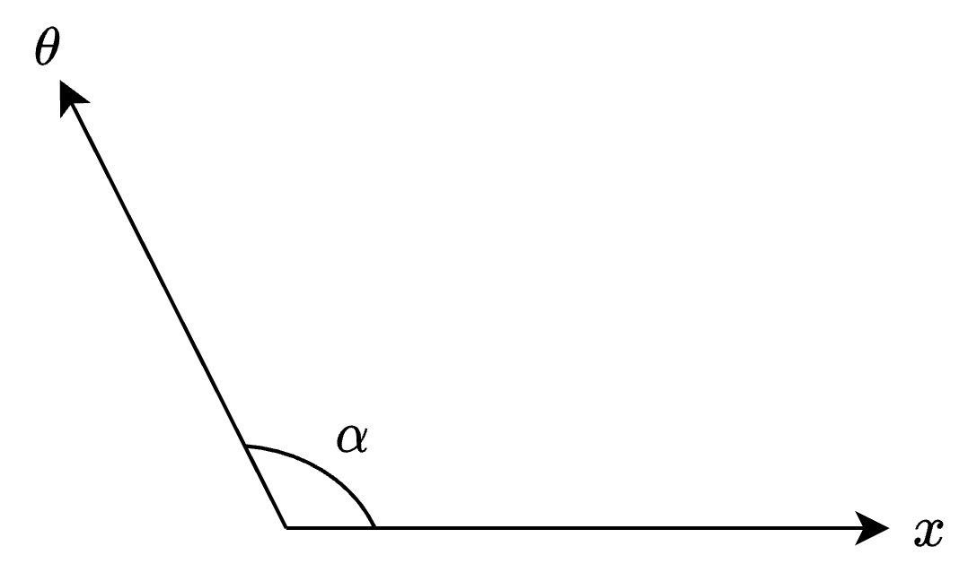
- If the angle between the vectors \(x\) and \(\theta\), denoted by \(\alpha\) is say \(>90^{\circ}\), then the vectors are not sufficiently correlated, since their dot product would be negative (since \(\cos(\theta) < 0\) for \(90^{\circ} < \theta < 270^{\circ}\)).
- Now, consider \(\theta’\) which is at an angle \(\beta <90^{\circ}\) to vector \(x\).
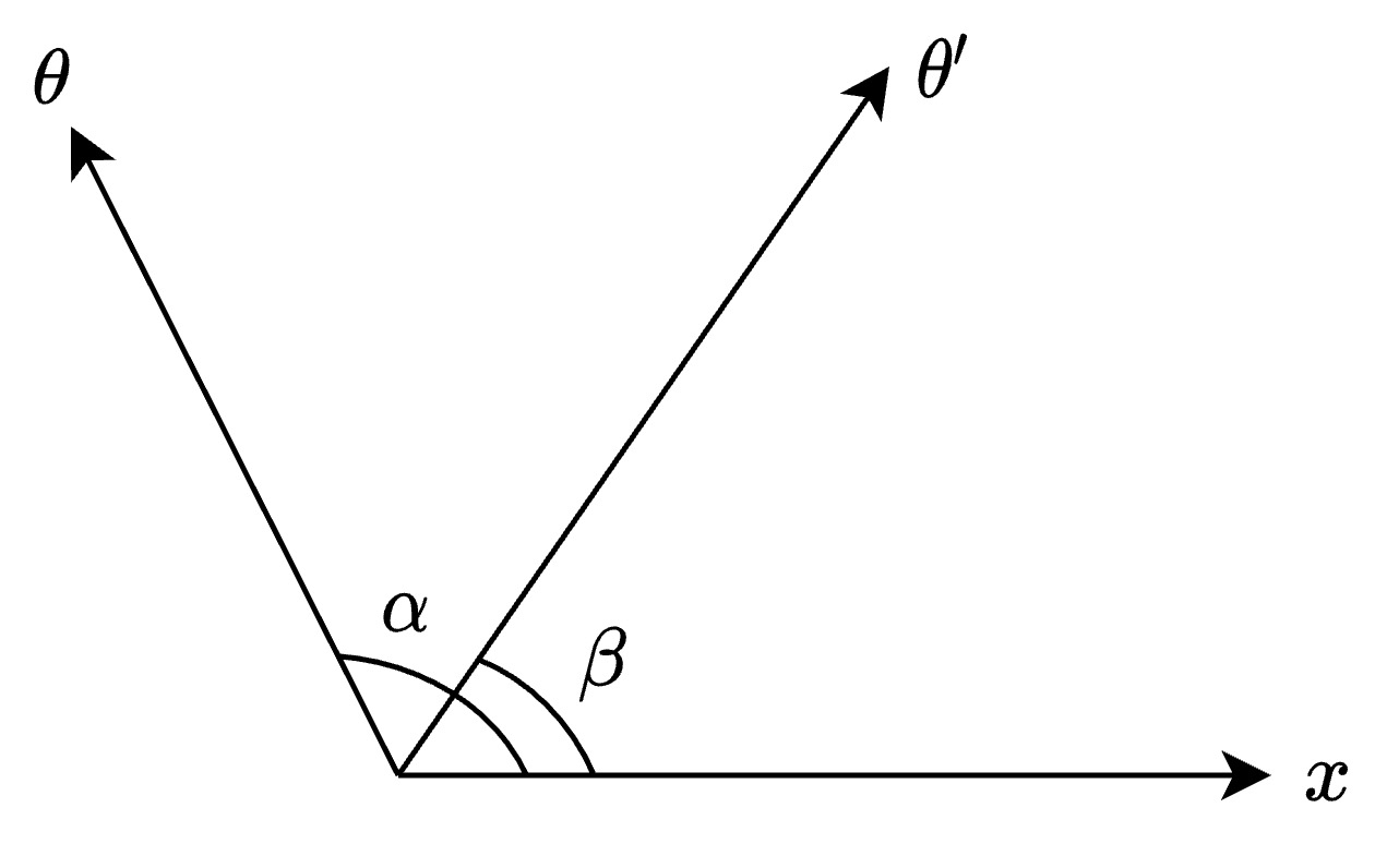
- The dot product between \(x\) and \(\theta’\) would be positive (since \(\cos(\theta) > 0\) for \(0^{\circ} \geq \theta < 90^{\circ}\)), increasing the correlation between the vectors.
- A simple way of making \(\theta\) closer to \(x\) (thereby increasing the correlation between the vectors) is to just add a component of \(x\) to \(\theta\).
- This is a very common technique used in lots of algorithms (especially NLP) where if you add a vector to another vector, you make the second one closer to the first one, and thereby increase the correlation between the two vectors.
Convergence
- Convergence with perceptrons can be achieved by annealing your learning rate with every step or using a learning rate schedule (varying the learning rate depending on the number of examples your algorithm has seen). Thus, you can introduce smaller and smaller changes to \(\theta\) as your algorithm sees more and more training samples.
Convergence is thus a design choice that the end-user needs to make depending on when they want to stop training.
Further reading
Here are some (optional) links you may find interesting for further reading:
- Learning in graphical models by Michael I. Jordan and Generalized Linear Models 2nd ed. by McCullagh and Nelder served as a major inspiration for our discussion on this topic.
- Wikipedia article on Perceptron.
References
Citation
If you found our work useful, please cite it as:
@article{Chadha2020DistilledPerceptron,
  title   = {Perceptron},
  author  = {Chadha, Aman},
  journal = {Distilled Notes for Stanford CS229: Machine Learning},
  year    = {2020},
  note    = {\url{https://aman.ai}}
}