Primers • Math
- Linear Algebra
- Plotting vectors
- Differential Calculus
- Slope of a straight line
- Defining the slope of a curve
- Differentiability
- Differentiating a function
- Differentiation rules
- Derivatives and optimization
- Higher order derivatives
- Partial derivatives
- Gradients
- Jacobians
- Hessians
- Examples
- Derivative 1: Composed Exponential Function
- Derivative 2. Function with Variable Base and Variable Exponent
- Derivative 3: Gradient of a Multi-Dimensional Input Function
- Derivative 4. Jacobian of a Multi-Dimensional Input and Output Function
- Derivative 5. Hessian of a Multi-Dimensional Input Function
- Probability theory
- Concepts
- Probability distributions
- Random Variables
- Central Limit Theorem
- Types of probability distributions
- Bernoulli distribution
- Gaussian/normal distribution
- Poisson distribution
- Uniform distribution
- Geometric distribution
- Student’s t-distribution
- Chi-squared distribution
- Exponential distribution
- F distribution
- Gamma distribution
- Beta distribution
- Frequentist inference
- Bayesian inference
- Regression Analysis
- Trigonometry
- References and Credits
- Citation

Linear Algebra
- Linear Algebra is the branch of mathematics that studies vector spaces and linear transformations between vector spaces, such as rotating a shape, scaling it up or down, translating it (i.e., moving it), etc.
- Machine Learning relies heavily on Linear Algebra, so it is essential to understand what vectors and matrices are, what operations you can perform with them, and how they can be useful.
Vectors
Definition
-
A vector is a quantity defined by a magnitude and a direction. For example, a rocket’s velocity is a 3-dimensional vector: its magnitude is the speed of the rocket, and its direction is (hopefully) up. A vector can be represented by an array of numbers called scalars. Each scalar corresponds to the magnitude of the vector with regards to each dimension.
-
For example, say the rocket is going up at a slight angle: it has a vertical speed of 5,000 m/s, and also a slight speed towards the East at 10 m/s, and a slight speed towards the North at 50 m/s. The rocket’s velocity may be represented by the following vector:
-
Note: by convention vectors are generally presented in the form of columns. Also, vector names are generally lowercase to distinguish them from matrices (which we will discuss below) and in bold (when possible) to distinguish them from simple scalar values such as \(meters\_per\_second = 5026\).
-
A list of \(N\) numbers may also represent the coordinates of a point in an \(N\)-dimensional space, so it is quite frequent to represent vectors as simple points instead of arrows. A vector with 1 element may be represented as an arrow or a point on an axis, a vector with 2 elements is an arrow or a point on a plane, a vector with 3 elements is an arrow or point in space, and a vector with \(N\) elements is an arrow or a point in an \(N\)-dimensional space… which most people find hard to imagine.
Purpose
- Vectors have many purposes in Machine Learning, most notably to represent observations and predictions. For example, say we built a Machine Learning system to classify videos into 3 categories (good, spam, clickbait) based on what we know about them. For each video, we would have a vector representing what we know about it, such as:
-
This vector could represent a video that lasts 10.5 minutes, but only 5.2% viewers watch for more than a minute, it gets 3.25 views per day on average, and it was flagged 7 times as spam. As you can see, each axis may have a different meaning.
-
Based on this vector our Machine Learning system may predict that there is an 80% probability that it is a spam video, 18% that it is click-bait, and 2% that it is a good video. This could be represented as the following vector:
Vectors in python
- In python, a vector can be represented in many ways, the simplest being a regular python list of numbers:
[10.5, 5.2, 3.25, 7.0]
- Since we plan to do quite a lot of scientific calculations, it is much better to use NumPy’s
ndarray, which provides a lot of convenient and optimized implementations of essential mathematical operations on vectors (for more details about NumPy, check out the NumPy tutorial). For example:
import numpy as np
video = np.array([10.5, 5.2, 3.25, 7.0])
video
- The size of a vector can be obtained using the
sizeattribute:
video.size
-
The \(i^{th}\) element (also called entry or item) of a vector \(\textbf{v}\) is noted \(\textbf{v}_i\).
-
Note that indices in mathematics generally start at 1, but in programming they usually start at 0. So to access \(\textbf{video}_3\) programmatically, we would write:
video[2] ## 3rd element
Plotting vectors
- To plot vectors, we will use matplotlib, so let’s start by importing it (for details about Matplotlib, check out our Matplotlib tutorial):
import matplotlib.pyplot as plt
- In a Jupyter/Colab notebook, we can simply output the graphs within the notebook itself by running the
%matplotlib inlinemagic command. Run this cell if you’re viewing this in Colab:
%matplotlib inline
2D vectors
- Now, import NumPy for array containers to handle the input data that we’re looking to plot:
import numpy as np
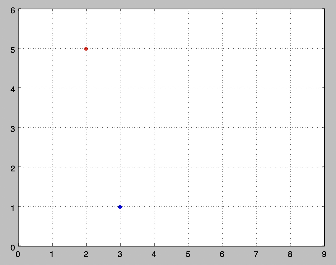
- Let’s create a couple very simple 2D vectors to plot:
u = np.array([2, 5])
v = np.array([3, 1])
- These vectors each have 2 elements, so they can easily be represented graphically on a 2D graph, for example as points:
x_coords, y_coords = zip(u, v)
plt.scatter(x_coords, y_coords, color=["r","b"])
plt.axis([0, 9, 0, 6])
plt.grid()
plt.show()
3D vectors
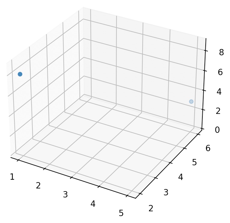
- Plotting 3D vectors is also relatively straightforward. First let’s create two 3D vectors:
import numpy as np

a = np.array([1, 2, 8])
b = np.array([5, 6, 3])
- Now let’s plot them using matplotlib’s
Axes3D. Note that we’ll be usingmpl_toolkitsto carry out this step (andmatplotlibdoes not loadmpl_toolkitsas a dependency during installation) so let’s load it up first usingpip install --upgrade matplotlib(if you’re running this in a Jupyter notebook, use!pip install --upgrade matplotlib).
import matplotlib.pyplot as plt
from mpl_toolkits.mplot3d import Axes3D

subplot3d = plt.subplot(111, projection='3d')
x_coords, y_coords, z_coords = zip(a,b)
subplot3d.scatter(x_coords, y_coords, z_coords)
subplot3d.set_zlim3d([0, 9])
plt.show()
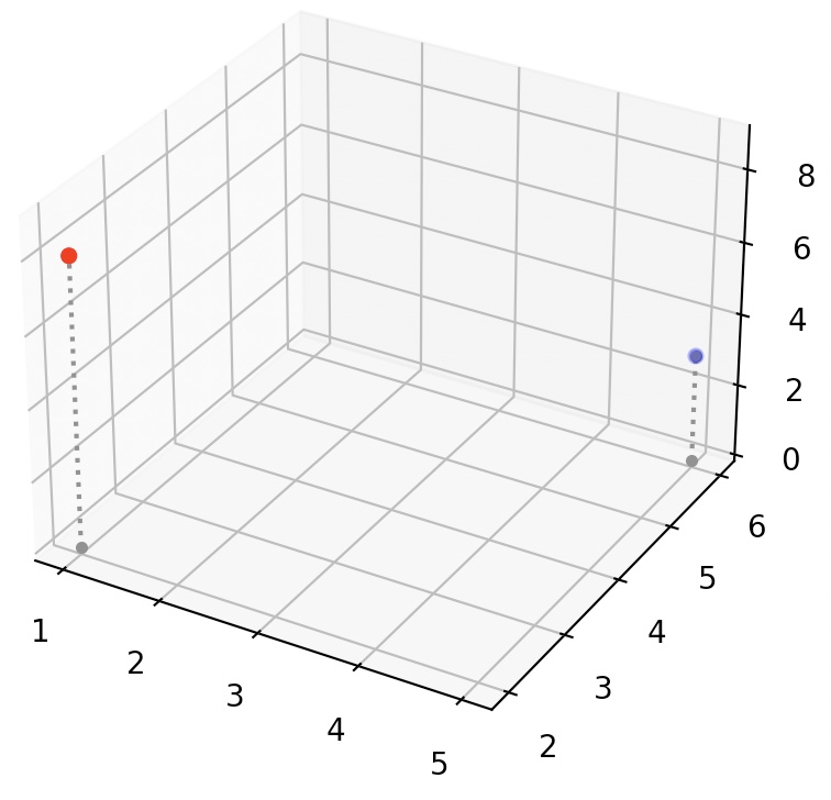
- It is a bit hard to visualize exactly where in space these two points are, so let’s add vertical lines. We’ll create a small convenience function to plot a list of 3D vectors with vertical lines attached:
def plot_vectors3d(ax, vectors3d, z0, **options):
    for v in vectors3d:
        x, y, z = v
        ax.plot([x,x], [y,y], [z0, z], color="gray", linestyle='dotted', marker=".")
    x_coords, y_coords, z_coords = zip(*vectors3d)
    ax.scatter(x_coords, y_coords, z_coords, **options)

subplot3d = plt.subplot(111, projection='3d')
subplot3d.set_zlim([0, 9])
plot_vectors3d(subplot3d, [a,b], 0, color=("r","b"))
plt.show()
Norm
- The norm of a vector \(\textbf{u}\), noted \(\mid \mid \textbf{u} \mid \mid \), is a measure of the length (a.k.a. the magnitude) of \(\textbf{u}\). There are multiple possible norms, but the most common one (and the only one we will discuss here) is the Euclidian norm, which is defined as:
- We could implement this easily in pure python, recalling that \(\sqrt x = x^{\frac{1}{2}}\).
def vector_norm(vector):
    squares = [element**2 for element in vector]
    return sum(squares)**0.5

u = np.array([2, 5])
print("||", u, "|| =")
vector_norm(u) # Prints 5.385164807134504
- However, it is much more efficient to use NumPy’s
normfunction, available in thelinalg(Linear Algebra) module:
import numpy.linalg as LA
LA.norm(u) # Prints 5.385164807134504
- Let’s plot a little diagram to confirm that the length of vector \(\textbf{v}\) is indeed \(\approx5.4\):
radius = LA.norm(u)
plt.gca().add_artist(plt.Circle((0,0), radius, color="#DDDDDD"))

def plot_vector2d(vector2d, origin=[0, 0], **options):
    return plt.arrow(origin[0], origin[1], vector2d[0], vector2d[1], head_width=0.2,
           head_length=0.3, length_includes_head=True, **options)

plot_vector2d(u, color="red")
plt.axis([0, 8.7, 0, 6])
plt.grid()
plt.show()
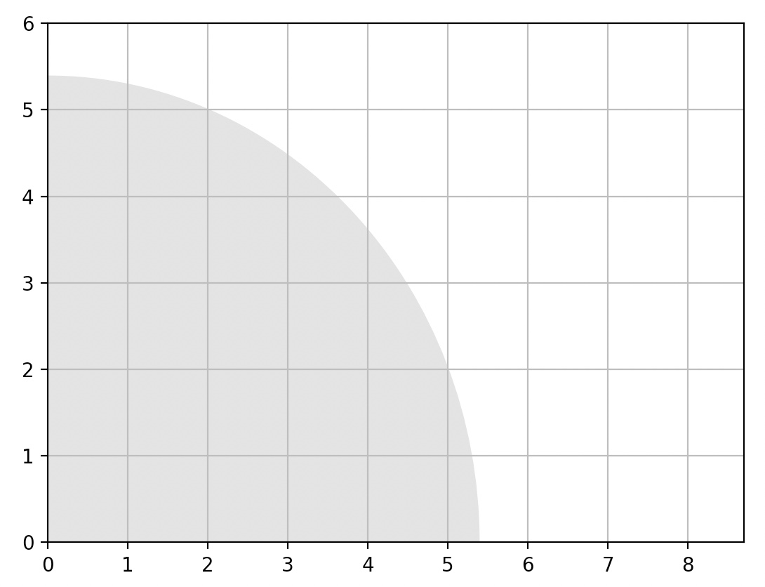
- Looks about right!
Addition
- Vectors of same size can be added together. Addition is performed elementwise:
import numpy as np

u = np.array([2, 5])
v = np.array([3, 1])

print(" ", u)
print("+", v)
print("-"*10)
u + v
- which outputs:
  [2 5]
+ [3 1]
----------
array([5, 6])
- Let’s look at what vector addition looks like graphically:
plot_vector2d(u, color="r")
plot_vector2d(v, color="b")
plot_vector2d(v, origin=u, color="b", linestyle="dotted")
plot_vector2d(u, origin=v, color="r", linestyle="dotted")
plot_vector2d(u+v, color="g")
plt.axis([0, 9, 0, 7])
plt.text(0.7, 3, "u", color="r", fontsize=18)
plt.text(4, 3, "u", color="r", fontsize=18)
plt.text(1.8, 0.2, "v", color="b", fontsize=18)
plt.text(3.1, 5.6, "v", color="b", fontsize=18)
plt.text(2.4, 2.5, "u+v", color="g", fontsize=18)
plt.grid()
plt.show()
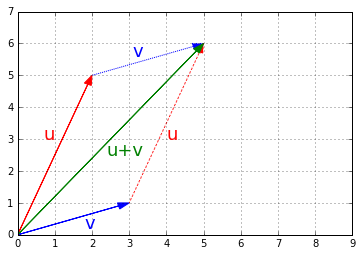
- Vector addition is commutative, meaning that \(\textbf{u} + \textbf{v} = \textbf{v} + \textbf{u}\). You can see it on the previous image: following \(\textbf{u}\) then \(\textbf{v}\) leads to the same point as following \(\textbf{v}\) then \(\textbf{u}\).
-
Vector addition is also associative, meaning that \(\textbf{u} + (\textbf{v} + \textbf{w}) = (\textbf{u} + \textbf{v}) + \textbf{w}\).
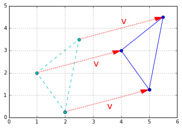
- If you have a shape defined by a number of points (vectors), and you add a vector \(\textbf{v}\) to all of these points, then the whole shape gets shifted by \(\textbf{v}\). This is called a geometric translation:
t1 = np.array([2, 0.25])
t2 = np.array([2.5, 3.5])
t3 = np.array([1, 2])

x_coords, y_coords = zip(t1, t2, t3, t1)
plt.plot(x_coords, y_coords, "c--", x_coords, y_coords, "co")

plot_vector2d(v, t1, color="r", linestyle=":")
plot_vector2d(v, t2, color="r", linestyle=":")
plot_vector2d(v, t3, color="r", linestyle=":")

t1b = t1 + v
t2b = t2 + v
t3b = t3 + v

x_coords_b, y_coords_b = zip(t1b, t2b, t3b, t1b)
plt.plot(x_coords_b, y_coords_b, "b-", x_coords_b, y_coords_b, "bo")

plt.text(4, 4.2, "v", color="r", fontsize=18)
plt.text(3, 2.3, "v", color="r", fontsize=18)
plt.text(3.5, 0.4, "v", color="r", fontsize=18)

plt.axis([0, 6, 0, 5])
plt.grid()
plt.show()
- Finally, subtracting a vector is like adding the opposite vector.
Differential Calculus
- Calculus is the study of continuous change. It has two major subfields: differential calculus, which studies the rate of change of functions, and integral calculus, which studies the area under the curve. In this notebook, we will discuss the former.
- Differential calculus is at the core of deep learning, so it is important to understand what derivatives and gradients are, how they are used in deep learning, and understand what their limitations are.
Slope of a straight line
- The slope of a (non-vertical) straight line can be calculated by taking any two points \(\mathrm{A}\) and \(\mathrm{B}\) on the line, and computing the “rise over run”:
- In this example, the height (rise) is 3, and the width (run) is 6, so the slope is \(\frac{3}{6} = 0.5\).

Defining the slope of a curve
- Now, let’s try to figure out how we can compute the slope of something else than a straight line. For example, let’s consider the curve defined by \(y = f(x) = x^2\):

-
Obviously, the slope varies: on the left (i.e., when \(x<0\)), the slope is negative (i.e., when we move from left to right, the curve goes down), while on the right (i.e., when \(x>0\)) the slope is positive (i.e., when we move from left to right, the curve goes up). At the point \(x=0\), the slope is equal to 0 (i.e., the curve is locally flat). The fact that the slope is 0 when we reach a minimum (or indeed a maximum) is crucially important, and we will come back to it later.
-
How can we put numbers on these intuitions? Well, say we want to estimate the slope of the curve at a point \(\mathrm{A}\), we can do this by taking another point \(\mathrm{B}\) on the curve, not too far away, and then computing the slope between these two points.
-
As you can see, when point \(\mathrm{B}\) is very close to point \(\mathrm{A}\), the \((\mathrm{AB})\) line becomes almost indistinguishable from the curve itself (at least locally around point \(\mathrm{A}\)). The \((\mathrm{AB})\) line gets closer and closer to the tangent line to the curve at point \(\mathrm{A}\): this is the best linear approximation of the curve at point \(\mathrm{A}\).
-
So it makes sense to define the slope of the curve at point \(\mathrm{A}\) as the slope that the \(\mathrm{(AB)}\) line approaches when \(\mathrm{B}\) gets infinitely close to \(\mathrm{A}\). This slope is called the derivative of the function \(f\) at \(x=x_\mathrm{A}\). For example, the derivative of the function \(f(x)=x^2\) at \(x=x_\mathrm{A}\) is equal to \(2x_\mathrm{A}\) (we will see how to get this result shortly), so on the graph above, since the point \(\mathrm{A}\) is located at \(x_\mathrm{A}=-1\), the tangent line to the curve at that point has a slope of \(-2\).
Differentiability
- Note that some functions are not quite as well-behaved as \(x^2\): for example, consider the function \(f(x)=|x|\), the absolute value of \(x\):
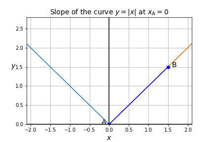
- No matter how much you zoom in on the origin (the point at \(x=0, y=0\)), the curve will always look like a V. The slope is -1 for any \(x < 0\), and it is +1 for any \(x > 0\), but at \(x = 0\), the slope is undefined, since it is not possible to approximate the curve \(y=|x|\) locally around the origin using a straight line, no matter how much you zoom in on that point.
- The function \(f(x)=|x|\) is said to be non-differentiable at \(x=0\): its derivative is undefined at \(x=0\). This means that the curve \(y=|x|\) has an undefined slope at that point. However, the function \(f(x)=|x|\) is differentiable at all other points.
-
In order for a function \(f(x)\) to be differentiable at some point \(x_\mathrm{A}\), the slope of the \((\mathrm{AB})\) line must approach a single finite value as \(\mathrm{B}\) gets infinitely close to \(\mathrm{A}\).
- This implies several constraints:
- First, the function must of course be defined at \(x_\mathrm{A}\). As a counterexample, the function \(f(x)=\dfrac{1}{x}\) is undefined at \(x_\mathrm{A}=0\), so it is not differentiable at that point.
- The function must also be continuous at \(x_\mathrm{A}\), meaning that as \(x_\mathrm{B}\) gets infinitely close to \(x_\mathrm{A}\), \(f(x_\mathrm{B})\) must also get infinitely close to \(f(x_\mathrm{A})\).
-
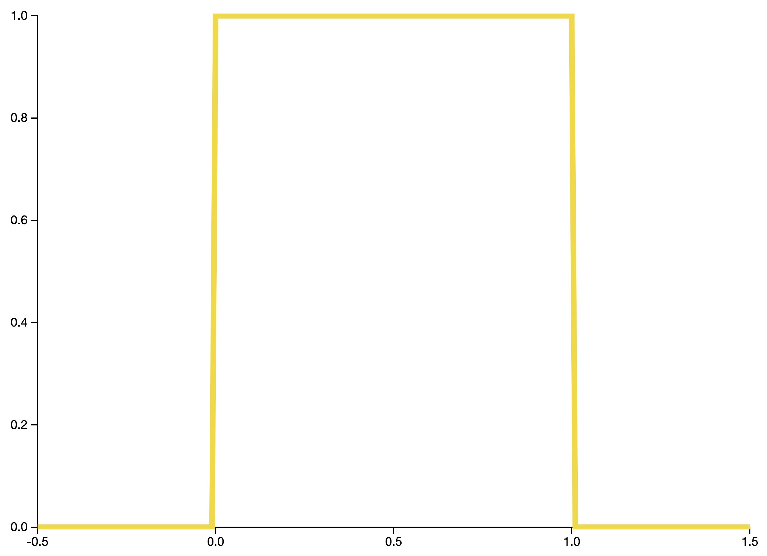
As a counterexample,
\[f(x)=\begin{cases}-1 \text{ if }x < 0\\+1 \text{ if }x \geq 0\end{cases}\]- is not continuous at \(x_\mathrm{A}=0\), even though it is defined at that point: indeed, when you approach it from the negative side, it does not approach infinitely close to \(f(0)=+1\). Therefore, it is not continuous at that point, and thus not differentiable either.
-
- The function must not have a breaking point at \(x_\mathrm{A}\), meaning that the slope that the \((\mathrm{AB})\) line approaches as \(\mathrm{B}\) approaches \(\mathrm{A}\) must be the same whether \(\mathrm{B}\) approaches from the left side or from the right side. We already saw a counterexample with \(f(x)=|x|\), which is both defined and continuous at \(x_\mathrm{A}=0\), but which has a breaking point at \(x_\mathrm{A}=0\): the slope of the curve \(y=|x|\) is -1 on the left, and +1 on the right.
- The curve \(y=f(x)\) must not be vertical at point \(\mathrm{A}\). One counterexample is \(f(x)=\sqrt[3]{x}\), the cubic root of \(x\): the curve is vertical at the origin, so the function is not differentiable at \(x_\mathrm{A}=0\).
Differentiating a function
- Now let’s see how to actually differentiate a function (i.e., find its derivative).
- The derivative of a function \(f(x)\) at \(x = x_\mathrm{A}\) is noted \(f’(x_\mathrm{A})\), and it is defined as:
- Don’t be scared, this is simpler than it looks! You may recognize the rise over run equation \(\dfrac{y_\mathrm{B} - y_\mathrm{A}}{x_\mathrm{B} - x_\mathrm{A}}\) that we discussed earlier. That’s just the slope of the \(\mathrm{(AB)}\) line. And the notation \(\underset{x_\mathrm{B} \to x_\mathrm{A}}\lim\) means that we are making \(x_\mathrm{B}\) approach infinitely close to \(x_\mathrm{A}\). So in plain English, \(f’(x_\mathrm{A})\) is the value that the slope of the \(\mathrm{(AB)}\) line approaches when \(\mathrm{B}\) gets infinitely close to \(\mathrm{A}\). This is just a formal way of saying exactly the same thing as earlier.
Example: finding the derivative of \(x^2\)
- Let’s look at a concrete example. Let’s see if we can determine what the slope of the \(y=x^2\) curve is, at any point \(\mathrm{A}\):
-
That’s it! We just proved that the slope of \(y = x^2\) at any point \(\mathrm{A}\) is \(f’(x_\mathrm{A}) = 2x_\mathrm{A}\). What we have done is called differentiation: finding the derivative of a function.
-
Note that we used a couple of important properties of limits. Here are the main properties you need to know to work with derivatives:
- \(\underset{x \to k}\lim c = c \quad\) if \(c\) is some constant value that does not depend on \(x\), then the limit is just \(c\).
- \(\underset{x \to k}\lim x = k \quad\) if \(x\) approaches some value \(k\), then the limit is \(k\).
- \(\underset{x \to k}\lim\,\left[f(x) + g(x)\right] = \underset{x \to k}\lim f(x) + \underset{x \to k}\lim g(x) \quad\) the limit of a sum is the sum of the limits
- \(\underset{x \to k}\lim\,\left[f(x) \times g(x)\right] = \underset{x \to k}\lim f(x) \times \underset{x \to k}\lim g(x) \quad\) the limit of a product is the product of the limits
- Important note: in Deep Learning, differentiation is almost always performed automatically by the framework you are using (such as TensorFlow or PyTorch). This is called auto-differentiation. However, you should still make sure you have a good understanding of derivatives, or else they will come and bite you one day, for example when you use a square root in your cost function without realizing that its derivative approaches infinity when \(x\) approaches 0 (tip: you should use \(\sqrt{x+\epsilon}\) instead, where \(\epsilon\) is some small constant, such as \(10^{-4}\)).
- You will often find a slightly different (but equivalent) definition of the derivative. Let’s derive it from the previous definition. First, let’s define \(\epsilon = x_\mathrm{B} - x_\mathrm{A}\). Next, note that \(\epsilon\) will approach 0 as \(x_\mathrm{B}\) approaches \(x_\mathrm{A}\). Lastly, note that \(x_\mathrm{B} = x_\mathrm{A} + \epsilon\). With that, we can reformulate the definition above like so:
- While we’re at it, let’s just rename \(x_\mathrm{A}\) to \(x\), to get rid of the annoying subscript A and make the equation simpler to read:
\[f'(x) = \underset{\epsilon \to 0}\lim\dfrac{f(x + \epsilon) - f(x)}{\epsilon}\]
- Okay! Now let’s use this new definition to find the derivative of \(f(x) = x^2\) at any point \(x\), and (hopefully) we should find the same result as above (except using \(x\) instead of \(x_\mathrm{A}\)):
- As we see, this result matches the result we obtained earlier.
Notations
- A word about notations: there are several other notations for the derivative that you will find in the litterature:
- This notation is also handy when a function is not named. For example \(\dfrac{\mathrm{d}}{\mathrm{d}x}[x^2]\) refers to the derivative of the function \(x \mapsto x^2\).
- Moreover, when people talk about the function \(f(x)\), they sometimes leave out “\((x)\)”, and they just talk about the function \(f\). When this is the case, the notation of the derivative is also simpler:
- The \(f’\) notation is Lagrange’s notation, while \(\dfrac{\mathrm{d}f}{\mathrm{d}x}\) is Leibniz’s notation.
- There are also other less common notations, such as Newton’s notation \(\dot y\) (assuming \(y = f(x)\)) or Euler’s notation \(\mathrm{D}f\).
Differentiation rules
-
One very important rule is that the derivative of a sum is the sum of the derivatives. More precisely, if we define \(f(x) = g(x) + h(x)\), then \(f’(x) = g’(x) + h’(x)\). This is quite easy to prove:
\[\begin{split} f'(x) && = \underset{\epsilon \to 0}\lim\dfrac{f(x+\epsilon) - f(x)}{\epsilon} && \quad\text{by definition}\\ && = \underset{\epsilon \to 0}\lim\dfrac{g(x+\epsilon) + h(x+\epsilon) - g(x) - h(x)}{\epsilon} && \quad \text{using }f(x) = g(x) + h(x) \\ && = \underset{\epsilon \to 0}\lim\dfrac{g(x+\epsilon) - g(x) + h(x+\epsilon) - h(x)}{\epsilon} && \quad \text{just moving terms around}\\ && = \underset{\epsilon \to 0}\lim\dfrac{g(x+\epsilon) - g(x)}{\epsilon} + \underset{\epsilon \to 0}\lim\dfrac{h(x+\epsilon) - h(x)}{\epsilon} && \quad \text{since the limit of a sum is the sum of the limits}\\ && = g'(x) + h'(x) && \quad \text{using the definitions of }g'(x) \text{ and } h'(x) \end{split}\] -
Similarly, it is possible to show the following important rules (I’ve included the proofs at the end of this notebook, in case you’re curious):
| Function \(f\) | Derivative \(f’\) | |
|---|---|---|
| Constant | \(f(x) = c\) | \(f’(x) = 0\) |
| Sum | \(f(x) = g(x) + h(x)\) | \(f’(x) = g’(x) + h’(x)\) |
| Product | \(f(x) = g(x) h(x)\) | \(f’(x) = g(x)h’(x) + g’(x)h(x)\) |
| Quotient | \(f(x) = \dfrac{g(x)}{h(x)}\) | \(f’(x) = \dfrac{g’(x)h(x) - g(x)h’(x)}{h^2(x)}\) |
| Power | \(f(x) = x^r\) with \(r \neq 0\) | \(f’(x) = rx^{r-1}\) |
| Exponential | \(f(x) = \exp(x)\) | \(f’(x)=\exp(x)\) |
| Logarithm | \(f(x) = \ln(x)\) | \(f’(x) = \dfrac{1}{x}\) |
| Sin | \(f(x) = \sin(x)\) | \(f’(x) = \cos(x)\) |
| Cos | \(f(x) = \cos(x)\) | \(f’(x) = -\sin(x)\) |
| Tan | \(f(x) = \tan(x)\) | \(f’(x) = \dfrac{1}{\cos^2(x)}\) |
| Chain Rule | \(f(x) = g(h(x))\) | \(f’(x) = g’(h(x))\,h’(x)\) |
- Let’s try differentiating a simple function using the above rules: we will find the derivative of \(f(x)=x^3+\cos(x)\). Using the rule for the derivative of sums, we find that \(f’(x)=\dfrac{\mathrm{d}}{\mathrm{d}x}[x^3] + \dfrac{\mathrm{d}}{\mathrm{d}x}[\cos(x)]\). Using the rule for the derivative of powers and for the \(\cos\) function, we find that \(f’(x) = 3x^2 - \sin(x)\).
- Let’s try a harder example: let’s find the derivative of \(f(x) = \sin(2 x^2) + 1\). First, let’s define \(u(x)=\sin(x) + 1\) and \(v(x) = 2x^2\). Using the rule for sums, we find that \(u’(x)=\dfrac{\mathrm{d}}{\mathrm{d}x}[sin(x)] + \dfrac{\mathrm{d}}{\mathrm{d}x}[1]\). Since the derivative of the \(\sin\) function is \(\cos\), and the derivative of constants is 0, we find that \(u’(x)=\cos(x)\). Next, using the product rule, we find that \(v’(x)=2\dfrac{\mathrm{d}}{\mathrm{d}x}[x^2] + \dfrac{\mathrm{d}}{\mathrm{d}x}[2]\,x^2\). Since the derivative of a constant is 0, the second term cancels out. And since the power rule tells us that the derivative of \(x^2\) is \(2x\), we find that \(v’(x)=4x\). Lastly, using the chain rule, since \(f(x)=u(v(x))\), we find that \(f’(x)=u’(v(x))\,v’(x)=\cos(2x^2)\,4x\).
The chain rule
- Refer our treatment of the chain rule here.
Derivatives and optimization
-
When trying to optimize a function \(f(x)\), we look for the values of \(x\) that minimize (or maximize) the function.
-
It is important to note that when a function reaches a minimum or maximum, assuming it is differentiable at that point, the derivative will necessarily be equal to 0. For example, you can check the above animation, and notice that whenever the function \(f\) (in the upper graph) reaches a maximum or minimum, then the derivative \(f’\) (in the lower graph) is equal to 0.
-
So one way to optimize a function is to differentiate it and analytically find all the values for which the derivative is 0, then determine which of these values optimize the function (if any). For example, consider the function \(f(x)=\dfrac{1}{4}x^4 - x^2 + \dfrac{1}{2}\). Using the derivative rules (specifically, the sum rule, the product rule, the power rule and the constant rule), we find that \(f’(x)=x^3 - 2x\). We look for the values of \(x\) for which \(f’(x)=0\), so \(x^3-2x=0\), and therefore \(x(x^2-2)=0\). So \(x=0\), or \(x=\sqrt2\) or \(x=-\sqrt2\). As you can see on the following graph of \(f(x)\), these 3 values correspond to local extrema. Two global minima \(f\left(\sqrt2\right)=f\left(-\sqrt2\right)=-\dfrac{1}{2}\) and one local maximum \(f(0)=\dfrac{1}{2}\).

- If a function has a local extremum at a point \(x_\mathrm{A}\) and is differentiable at that point, then \(f’(x_\mathrm{A})=0\). However, the reverse is not always true. For example, consider \(f(x)=x^3\). Its derivative is \(f’(x)=x^2\), which is equal to 0 at \(x_\mathrm{A}=0\). Yet, this point is not an extremum, as you can see on the following diagram. It’s just a single point where the slope is 0.

- So in short, you can optimize a function by analytically working out the points at which the derivative is 0, and then investigating only these points. It’s a beautifully elegant solution, but it requires a lot of work, and it’s not always easy, or even possible. For neural networks, it’s practically impossible.
- Another option to optimize a function is to perform Gradient Descent (we will consider minimizing the function, but the process would be almost identical if we tried to maximize a function instead): start at a random point \(x_0\), then use the function’s derivative to determine the slope at that point, and move a little bit in the downwards direction, then repeat the process until you reach a local minimum, and cross your fingers in the hope that this happens to be the global minimum.
- At each iteration, the step size is proportional to the slope, so the process naturally slows down as it approaches a local minimum. Each step is also proportional to the learning rate: a parameter of the Gradient Descent algorithm itself (since it is not a parameter of the function we are optimizing, it is called a hyperparameter).
Higher order derivatives
- What happens if we try to differentiate the function \(f\prime(x)\)? Well, we get the so-called second order derivative, noted \(f\prime\prime(x)\), or \(\dfrac{\mathrm{d}^2f}{\mathrm{d}x^2}\). If we repeat the process by differentiating \(f\prime\prime(x)\), we get the third-order derivative \(f\prime\prime\prime(x)\), or \(\dfrac{\mathrm{d}^3f}{\mathrm{d}x^3}\). And we could go on to get higher order derivatives.
- What’s the intuition behind second order derivatives? Well, since the (first order) derivative represents the instantaneous rate of change of \(f\) at each point, the second order derivative represents the instantaneous rate of change of the rate of change itself, in other words, you can think of it as the acceleration of the curve: if \(f\prime\prime(x) < 0\), then the curve is accelerating “downwards”, if \(f\prime\prime(x) > 0\) then the curve is accelerating “upwards”, and if \(f\prime\prime(x) = 0\), then the curve is locally a straight line. Note that a curve could be going upwards (i.e., \(f\prime(x)>0\)) but also be accelerating downwards (i.e., \(f\prime\prime(x) < 0\)): for example, imagine the path of a stone thrown upwards, as it is being slowed down by gravity (which constantly accelerates the stone downwards).
- Deep Learning generally only uses first order derivatives, but you will sometimes run into some optimization algorithms or cost functions based on second order derivatives.
Partial derivatives
- Up to now, we have only considered functions with a single variable \(x\). What happens when there are multiple variables? For example, let’s start with a simple function with 2 variables: \(f(x,y)=\sin(xy)\). If we plot this function, using \(z=f(x,y)\), we get the following 3D graph. I also plotted some point \(\mathrm{A}\) on the surface, along with two lines I will describe shortly.

- If you were to stand on this surface at point \(\mathrm{A}\) and walk along the \(x\) axis towards the right (increasing \(x\)), your path would go down quite steeply (along the dashed blue line). The slope along this axis would be negative. However, if you were to walk along the \(y\) axis, towards the back (increasing \(y\)), then your path would almost be flat (along the solid red line), at least locally: the slope along that axis, at point \(\mathrm{A}\), would be very slightly positive.
- As you can see, a single number is no longer sufficient to describe the slope of the function at a given point. We need one slope for the \(x\) axis, and one slope for the \(y\) axis. One slope for each variable. To find the slope along the \(x\) axis, called the partial derivative of \(f\) with regards to \(x\), and noted \(\dfrac{\partial f}{\partial x}\) (with curly \(\partial\)), we can differentiate \(f(x,y)\) with regards to \(x\) while treating all other variables (in this case just \(y\)) as constants:
- If you use the derivative rules listed earlier (in this example you would just need the product rule and the chain rule), making sure to treat \(y\) as a constant, then you will find:
- Similarly, the partial derivative of \(f\) with regards to \(y\) is defined as:
- All variables except for \(y\) are treated like constants (just \(x\) in this example). Using the derivative rules, we get:
- We now have equations to compute the slope along the \(x\) axis and along the \(y\) axis. But what about the other directions? If you were standing on the surface at point \(\mathrm{A}\), you could decide to walk in any direction you choose, not just along the \(x\) or \(y\) axes. What would the slope be then? Shouldn’t we compute the slope along every possible direction?
- Well, it can be shown that if all the partial derivatives are defined and continuous in a neighborhood around point \(\mathrm{A}\), then the function \(f\) is totally differentiable at that point, meaning that it can be locally approximated by a plane \(P_\mathrm{A}\) (the tangent plane to the surface at point \(\mathrm{A}\)). In this case, having just the partial derivatives along each axis ($x\) and \(y\) in our case) is sufficient to perfectly characterize that plane. Its equation is:
- In Deep Learning, we will generally be dealing with well-behaved functions that are totally differentiable at any point where all the partial derivatives are defined, but you should know that some functions are not that nice. For example, consider the function:
- At the origin (i.e., at \((x,y)=(0,0)\)), the partial derivatives of the function \(h\) with respect to \(x\) and \(y\) are both perfectly defined: they are equal to 0. Yet the function can clearly not be approximated by a plane at that point. It is not totally differentiable at that point (but it is totally differentiable at any point off the axes).
Gradients
- So far we have considered only functions with a single variable \(x\), or with 2 variables, \(x\) and \(y\), but the previous paragraph also applies to functions with more variables. So let’s consider a function \(f\) with \(n\) variables: \(f(x_1, x_2, \dots, x_n)\). For convenience, we will define a vector \(X\) whose components are these variables:
- Now \(f(X)\) is easier to write than \(f(x_1, x_2, \dots, x_n)\).
- The gradient of the function \(f(X)\) at some point \(X_\mathrm{A}\) is the vector whose components are all the partial derivatives of the function at that point. It is noted \(\nabla f(X_\mathrm{A})\), or sometimes \(\nabla_{X_\mathrm{A}}f\):
- Assuming the function is totally differentiable at the point \(X_A\), then the surface it describes can be approximated by a plane at that point (as discussed in the previous section), and the gradient vector is the one that points towards the steepest slope on that plane.
Gradient Descent, revisited
- In Deep Learning, the Gradient Descent algorithm we discussed earlier is based on gradients instead of derivatives (hence its name). It works in much the same way, but using vectors instead of scalars: simply start with a random vector \(X_{0}\), then compute the gradient of \(f\) at that point, and perform a small step in the opposite direction, then repeat until convergence. More precisely, at each step \(t\), compute \(X_t = X_{t-1} - \eta \nabla f(X_{t-1})\). The constant \(\eta\) is the learning rate, typically a small value such as \(10^{-3}\). In practice, we generally use more efficient variants of this algorithm, but the general idea remains the same.
- In Deep Learning, the letter \(X\) is generally used to represent the input data. When you use a neural network to make predictions, you feed the neural network the inputs \(X\), and you get back a prediction \(\hat{y} = f(X)\). The function \(f\) treats the model parameters as constants. We can use more explicit notation by writing \(\hat{y} = f_w(X)\), where \(w\) represents the model parameters and indicates that the function relies on them, but treats them as constants.
- However, when training a neural network, we do quite the opposite: all the training examples are grouped in a matrix \(X\), all the labels are grouped in a vector \(y\), and both \(X\) and \(y\) are treated as constants, while \(w\) is treated as variable: specifically, we try to minimize the cost function \(\mathcal L_{X, y}(w) = g(f_{X}(w), y)\), where \(g\) is a function that measures the “discrepancy” between the predictions \(f_{X}(w)\) and the labels \(y\), where \(f_{X}(w)\) represents the vector containing the predictions for each training example. Minimizing the loss function is usually performed using Gradient Descent (or a variant of GD): we start with random model parameters \(w_{0}\), then we compute \(\nabla \mathcal L(w_0)\) and we use this gradient vector to perform a Gradient Descent step, then we repeat the process until convergence. It is crucial to understand that the gradient of the loss function is with regards to the model parameters \(w\) (not the inputs \(X\)).
Jacobians
- Until now we have only considered functions that output a scalar, but it is possible to output vectors instead. For example, a classification neural network typically outputs one probability for each class, so if there are \(m\) classes, the neural network will output an \(d\)-dimensional vector for each input.
- In Deep Learning we generally only need to differentiate the loss function, which almost always outputs a single scalar number. But suppose for a second that you want to differentiate a function \(f(X)\) which outputs \(d\)-dimensional vectors. The good news is that you can treat each output dimension independently of the others. This will give you a partial derivative for each input dimension and each output dimension. If you put them all in a single matrix, with one column per input dimension and one row per output dimension, you get the so-called Jacobian matrix.
- The partial derivatives themselves are often called the Jacobians. It’s just the first order partial derivatives of the function \(f\).
Hessians
- Let’s come back to a function \(f(X)\) which takes an \(n\)-dimensional vector as input and outputs a scalar. If you determine the equation of the partial derivative of \(f\) with regards to \(x_i\) (the \(i^\text{th}\) component of \(X\)), you will get a new function of \(X\): \(\dfrac{\partial f}{\partial x_i}\). You can then compute the partial derivative of this function with regards to \(x_j\) (the \(j^\text{th}\) component of \(X\)). The result is a partial derivative of a partial derivative: in other words, it is a second order partial derivatives, also called a Hessian. It is noted \(X\): \(\dfrac{\partial^2 f}{\partial x_jx_i}\). If \(i\neq j\) then it is called a mixed second order partial derivative. Or else, if \(j=i\), it is noted \(\dfrac{\partial^2 f}{\partial {x_i}^2}\).
-
Let’s look at an example: \(f(x, y)=\sin(xy)\). As we showed earlier, the first order partial derivatives of \(f\) are: \(\dfrac{\partial f}{\partial x}=y\cos(xy)\) and \(\dfrac{\partial f}{\partial y}=x\cos(xy)\). So we can now compute all the Hessians (using the derivative rules we discussed earlier):
- \(\dfrac{\partial^2 f}{\partial x^2} = \dfrac{\partial f}{\partial x}\left[y\cos(xy)\right] = -y^2\sin(xy)\)
- \(\dfrac{\partial^2 f}{\partial y\,\partial x} = \dfrac{\partial f}{\partial y}\left[y\cos(xy)\right] = \cos(xy) - xy\sin(xy)\)
- \(\dfrac{\partial^2 f}{\partial x\,\partial y} = \dfrac{\partial f}{\partial x}\left[x\cos(xy)\right] = \cos(xy) - xy\sin(xy)\)
- \(\dfrac{\partial^2 f}{\partial y^2} = \dfrac{\partial f}{\partial y}\left[x\cos(xy)\right] = -x^2\sin(xy)\)
- Note that \(\dfrac{\partial^2 f}{\partial x\,\partial y} = \dfrac{\partial^2 f}{\partial y\,\partial x}\). This is the case whenever all the partial derivatives are defined and continuous in a neighborhood around the point at which we differentiate.
- The matrix containing all the Hessians is called the Hessian matrix:
- There are great optimization algorithms which take advantage of the Hessians, but in practice Deep Learning almost never uses them. Indeed, if a function has \(n\) variables, there are \(n^2\) Hessians: since neural networks typically have several millions of parameters, the number of Hessians would exceed thousands of billions. Even if we had the necessary amount of RAM, the computations would be prohibitively slow.
Examples
Derivative 1: Composed Exponential Function
\[f(x)=e^{x^{2}}, x \in \mathbb{R}\]- The exponential function is a very foundational, common, and useful example. It is a strictly positive function, i.e. \(e^{x}>0\) in \(\mathbb{R}\), and an important property to remember is that \(e^{0}=1 .\) In addition, you should remember that the exponential is the inverse of the logarithmic function. It is also one of the easiest functions to derivate because its derivative is simply the exponential itself, i.e. \(\left(e^{x}\right)^{\prime}=e^{x}\). The derivative becomes tricker when the exponential is combined with another function. In such cases, we use the chain rule formula, which states that the derivative of \(f(g(x))\) is equal to \(f^{\prime}(g(x)) \cdot g^{\prime}(x)\), i.e.,
- Applying chain rule, we can compute the derivative of \(f(x)=e^{x^{2}}\). We first Multiplying these two intermediate results, we obtain,
Derivative 2. Function with Variable Base and Variable Exponent
\[f(x)=x^{x}, x \in \mathbb{R}_{+}^{\ast}\]-
This function is a classic in interviews, especially in the financial/quant industry, where math skills are tested in even greater depth than in tech companies for machine learning positions. It sometimes brings the interviewees out of their comfort zone, but really, the hardest part of this question is to be able to start correctly.
-
The most important thing to realize when approaching a function in such exponential form is, first, the inverse relationship between exponential and logarithm, and, second, the fact, that every exponential function can be rewritten as a natural exponential function in the form of,
- Before we get to our \(f(x)=x^{\ast}\) example, let us demonstrate this property with a simpler function \(f(x)=2^{x}.\) We first use the above equation to rewrite \(2^{\ast}\) as \(\operatorname{exp}(x \ln (2))\) and subsequently apply chain rule.
- Going back to the original function \(f(x)=x^{x}\), once you rewrite the function as \(f(x)=\exp (x \ln x)\), the derivative becomes relatively straightforward to compute, with the only potentially difficult part being the chain rule step.
-
Note that here we used the product rule \((u v)^{\prime}=u^{\prime} v+u v^{\prime}\) for the exponent \(\sin (x)\).
-
This function is generally asked without any information on the function’s domain. If your interviewer doesn’t specify the domain by default, he might be testing your mathematical acuity. Here is where the question gets deceiving. Without being specific about the domain, it seems that \(x^{x}\) is defined for both positive and negative values. However, for negative \(x\), e.g. \((-0.9)^{\wedge}(-0.9)\), the result is a complex number, concretely \(-1.05-0.34 i . \mathrm{A}\) potential way out would be to define the domain of the function as \(\mathbb{Z}^{-} \cup \mathbb{R}^{+} \backslash 0\) (see here for further discussion), but this would still not be differentiable for negative values. Therefore, in order to properly define the derivative of \(x^{x}\), we need to restrict the domain to only strictly positive values. We exclude 0 because for a derivative to be defined in 0, we need the limit derivative from the left (limit in 0 for negative values) to be equal to the limit derivative from the right (limit in 0 for positive values) \(-\) a condition that is broken in this case. since the left limit \(\lim _{\Delta x \rightarrow 0^{-}} \frac{f(0+\Delta x)-f(0)}{\Delta x}\) is undefined, the function is not differentiable in 0, and thus the function’s domain is restricted to only positive values.
-
Before we move on to the next section, I leave you with a slightly more advanced version of this function to test your understanding: \(f(x)=x^{x^{2}}\). If you understood the logic and steps behind the first example, adding the extra exponent shouldn’t cause any difficulties and you should conclude the following result:
Derivative 3: Gradient of a Multi-Dimensional Input Function
\[f(x, y, z)=2^{x y}+z \cos (x),(x, y, z) \in \mathbb{R}^{3}\]-
So far, the functions discussed in the first and second derivative sections are functions mapping from \(\mathbb{R}\) to \(\mathbb{R}\), L. the domain as well as the range of the function are real numbers. But machine learning is essentially vectorial and the functions are multi-dimensional. A good example of such multidimensionality is a neural network layer of input size \(m\) and output size \(k\), i.e., \(f(x)=g\left(W^{\top} x+b\right)\), which is an element-wise composition of \(a_{2}\) linear mapping \(W^{T} x\) (with weight matrix \(W\) and input vector \(x\)) and a non linear mapping \(g\) (activation function). In the general case, this can also be viewed as a mapping from \(R^{m}\) to \(\mathbb{R}^{k}\).
-
In the specific case of \(k=1\), the derivative is called gradient. Let us now compute the derivative of the following three-dimensional function mapping \(\mathbb{R}^{3}\) to \(\mathbb{R}\):
-
You can think off as a function mapping a vector of size 3 to a vector of size 1
- The derivative of a multi-dimensional input function is called a gradient function \(g\) that maps \(\mathbb{R}^{n}\) to \(\mathbb{R}\) is a set of \(n\) partial derivatives of \(g\) where each \(h\) partial derivative is a function of \(n\) variables. Thus, if 8 is a mapping from \(\mathbb{R}^{\mathrm{D}}\) to \(\mathbb{R}\), its gradient \(\nabla g\) is a mapping from \(\mathbb{R}^{n}\) to \(\mathbb{R}^{n}\).
- To find the gradient of our function \(f(x, y, z)=2 w+z \cos (x)\), we construct vector of partial derivatives \(\partial f / \partial x\), f// \(\partial y\) and \(\partial f / \partial z\), and obtain the following result:
- Note that this is an example similar to the previous section and we use the equivalence \(2^{x y}=\exp (x y \ln (2))\).
- In conclusion, for a multi-dimensional function that maps \(\mathbb{R}^{3}\) to \(\mathbb{R}\), the derivative is a gradient \(\nabla f\), which maps \(\mathbb{R}^{3}\) to \(\mathbb{R}^{3}\).
- In a general form of mappings \(\mathbb{R}\) “to \(\mathbb{R}^{k}\) where \(k>1\), the derivative of a multi-dimensional function that maps \(\mathbb{R}^{\text {m }}\) to \(\mathbb{R}^{\text {k }}\) is a Jacobian matrix (instead of a gradient vector). Let us investigate this in the next section.
Derivative 4. Jacobian of a Multi-Dimensional Input and Output Function
\[f(x, y)=\left[\begin{array}{c} 2 x^{2} \\ x \sqrt{y} \end{array}\right], x \in \mathbb{R}, y \in \mathbb{R}^{+}\]- We know from the previous section that the derivative of a function mapping \(\mathbb{R}^{\text {m }}\) to \(\mathbb{R}\) is a gradient mapping \(\mathbb{R}\) “to \(\mathbb{R}\) “. But what about the case where also the output domain is multi-dimensional, i.e. a mapping from \(\mathbb{R}^{\text {m }}\) to \(\mathbb{R}^{k}\) for \(k>1\)?
- In such case, the derivative is called Jacobian matrix. We can view the gradient simply as a special case of Jacobian with dimension \(m \times 1\) with \(m\) equal to the number of variables. The Jacobian \(J(g)\) of a function \(g\) mapping \(\mathbb{R}^{\text {m to }}\) R a dimension of \(k \times m\), l.e. is a matrix of shape \(k \times m\). In other words, each row \(i\) of \(J(g)\) represents the gradient \(\nabla g_{i}\) of each sub-function \(g_{i}\) of \(g\).
- Let us derive the above defined function \(f(x, y)=\left[2 x^{2}, x \mid y\right]\) mapping \(\mathbb{R}^{2}\) to \(\mathbb{R}^{2}\), thus both input and output domains are multidimensional. In this particular case, since the square root function is not defined for negative values, we need to restrict the domain of \(y\) to \(\mathbb{R}^{+}\). The first row of our output Jacobian will be the derivative of function 1, i.e. \(\nabla 2 x^{2}\), and the second row the derivative of function 2, i.e. \(\nabla x \sqrt{y}\).
- In deep learning, an example where the Jacobian is of special interest is in the explainability field (see, for example, Sensitivity based Neural Networks Explanations) that aims to understand the behavior of neural networks and analyses sensitivity of the output layer of neural networks with regard to the inputs. The Jacobian helps to investigate the impact of variation in the input space on the output. This can analogously be applied to understand the concepts of intermediate layers in neural networks.
- In summary, remember that while gradient is a derivative of a scalar with regard to a vector, Jacobian is a derivative of a vector with regard to another vector.
Derivative 5. Hessian of a Multi-Dimensional Input Function
\[f(x, y)=x^{2} y^{3},(x, y) \in \mathbb{R}^{2}\]- So far, our discussion has only been focused on first-order derivatives, but in neural networks we often talk about higher-order derivatives of multidimensional functions. A specific case is the second derivative, also called the Hessian matrix, and denoted \(H(f)\) or \(\nabla^{2}\) (nabla squared). The Hessian of a function \(g\) mapping \(\mathbb{R}^{n}\) to \(\mathbb{R}\) is a mapping \(H(g)\) from \(\mathbb{R}^{n}\) to \(\mathbb{R}^{n * n}\).
- Let us analyze how we went from \(\mathbb{R}\) to \(\mathbb{R}^{n * n}\) on the output domain. The first derivative, i.e. gradient \(\nabla g\), is a mapping from \(\mathbb{R}^{n}\) to \(\mathbb{R}^{n}\) and its derivative is a Jacobian. Thus, the derivation of each sub-function \(\nabla g_{i}\) results in a mapping of \(\mathbb{R}^{n}\) to \(\mathbb{R}^{n}\), with \(n\) such functions. You can think of this as if deriving each element of the gradient vector expanded into a vector, becoming thus a vector of vectors, i.e. a matrix.
- To compute the Hessian, we need to calculate so-called cross-derivatives, that is, derivate first with respect to \(x\) and then with respect to \(y\), or vice-versa. One might ask if the order in which we take the cross derivatives matters; in other words, if the Hessian matrix is symmetric or not. In cases where the function \(f\) is \(\mathscr{C}^{2}\), i.e. twice continuously differentiable, Schwarz theorem states that the cross derivatives are equal and thus the Hessian matrix is symmetric. Some discontinuous, yet differentiable functions, do not satisfy the equality of cross-derivatives.
- Constructing the Hessian of a function is equal to finding second-order partial derivatives of a scalar-valued function. For the specific example \(f(x, y)=x^{2} y^{3}\), the computation yields the following result:
- You can see that the cross-derivatives \(6 x y^{2}\) are in fact equal. We first derived with regard to \(x\) and obtained \(2 x y^{3}\), then again with regard to \(y\), obtaining \(6 x y^{2} .\) The diagonal elements are simply \(f_{i}\) “ for each mono-dimensional subfunction of either \(x\) or \(y\).
- An extension would be to discuss the case of a second order derivatives for multi-dimensional functions mapping \(\mathbb{R}\) m to \(\mathbb{R}^{\text {k }}\), which can intuitively be seen as a second-order Jacobian. This is a mapping from \(\mathbb{R}^{\mathrm{m}}\) to \(\mathbb{R}^{\mathrm{k} * \mathrm{m}} * \mathrm{m}\), i.e. a 3D tensor. Similarly to the Hessian, in order to find the gradient of the Jacobian (differentiate a second time), we differentiate each element of the \(k \times m\) matrix and obtain a matrix of vectors, i.e. a tensor. While it is rather unlikely that you would be asked to do such computation manually, it is important to be aware of higher-order derivatives for multidimensional functions.
Probability theory
Concepts
Chance events
- Randomness is all around us. Probability theory is the mathematical framework that allows us to analyze chance events in a logically sound manner. The probability of an event is a number indicating how likely that event will occur. This number is always between 0 and 1, where 0 indicates impossibility and 1 indicates certainty.
- A classic example of a probabilistic experiment is a fair coin toss, in which the two possible outcomes are heads or tails. In this case, the probability of flipping a head or a tail is \(\frac{1}{2}\). In an actual series of coin tosses, we may get more or less than exactly 50% heads. But as the number of flips increases, the long-run frequency of heads is bound to get closer and closer to 50%.
- For an unfair or weighted coin, the two outcomes are not equally likely, in which case, you’ll need to assign appropriate weights to each of the outcomes. If we assign numbers to the outcomes — say, 1 for heads, 0 for tails — then we have created the mathematical object known as a random variable.
Expectation
- The expectation of a random variable is a number that attempts to capture the center of that random variable’s distribution. It can be interpreted as the long-run average of many independent samples from the given distribution. More precisely, it is defined as the probability-weighted sum of all possible values in the random variable’s support,
- Consider the probabilistic experiment of rolling a fair die. After a sufficiently large number of iterations, the running sample mean converges to the expectation of 3.5. Changing the distribution of the different faces of the die (thus making the die biased or “unfair”) would affect the expected value.
Variance
- Whereas expectation provides a measure of centrality, the variance of a random variable quantifies the spread of that random variable’s distribution. The variance is the average value of the squared difference between the random variable and its expectation,
- When you draw cards randomly from a deck of ten cards, you’ll observe that the running average of squared differences begins to resemble the true variance.
Set Theory
- A set, broadly defined, is a collection of objects. In the context of probability theory, we use set notation to specify compound events. For example, we can represent the event “roll an even number” by the set \(\{2, 4, 6\}\). For this reason it is important to be familiar with the algebra of sets.
- Sets are usually visualized as Venn diagrams.
Counting
- It can be surprisingly difficult to count the number of sequences or sets satisfying certain conditions.
- For example, consider a bag of marbles in which each marble is a different color. If we draw marbles one at a time from the bag without replacement, and there exists four unique marbles in the bag, how many different ordered sequences (permutations) of the marbles are possible? How many different unordered sets (combinations)?
- Permutations with \(n = 4\) and \(^nP_{x} = 1\):
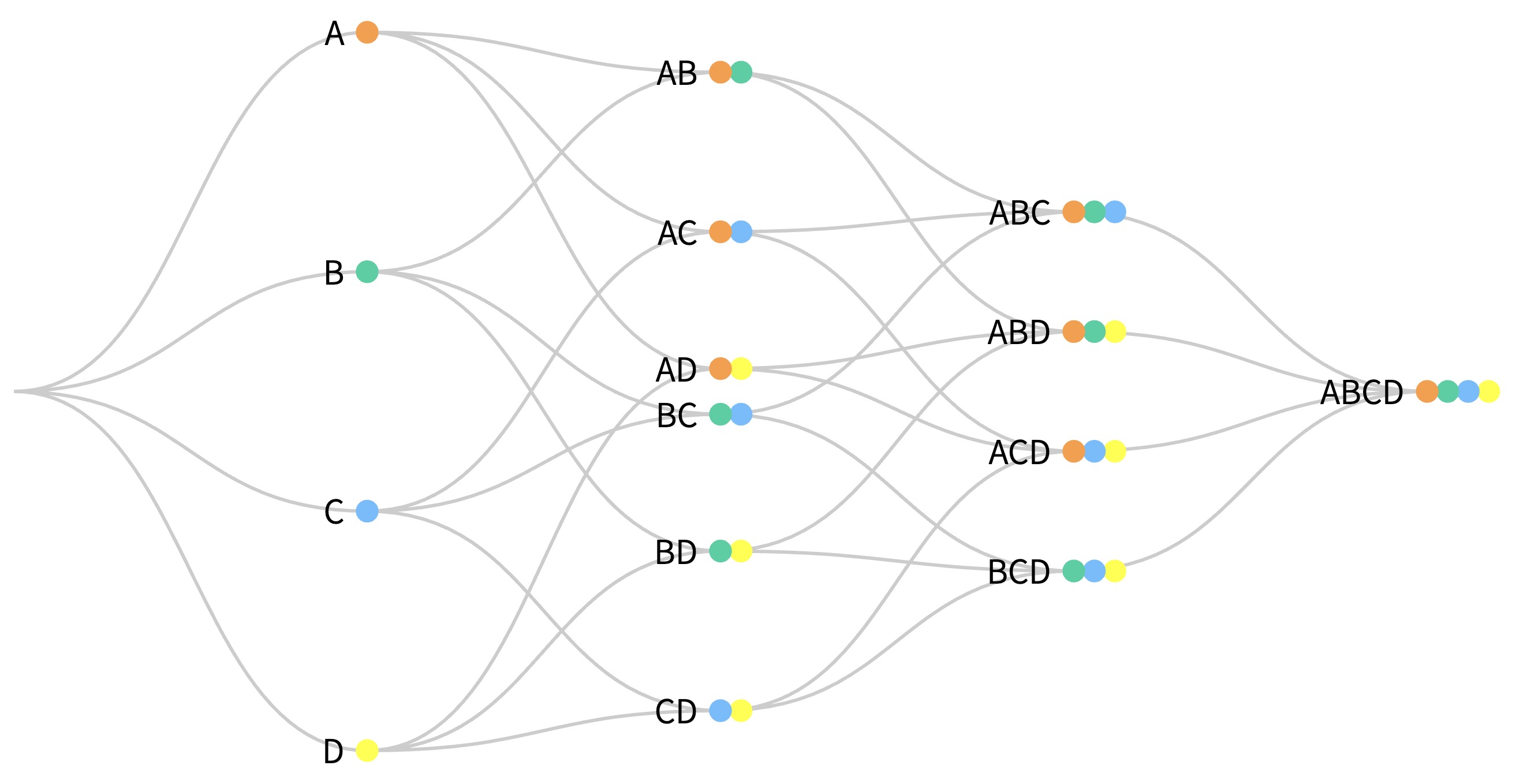
- Combinations with \(n = 4\) and \({n \choose x}\) or \(^nC_{x} = 1\):
Conditional Probability
- Conditional probabilities allow us to account for information we have about our system of interest. For example, we might expect the probability that it will rain tomorrow (in general) to be smaller than the probability it will rain tomorrow given that it is cloudy today. This latter probability is a conditional probability, since it accounts for relevant information that we possess.
- Mathematically, computing a conditional probability amounts to shrinking our sample space to a particular event. So in our rain example, instead of looking at how often it rains on any day in general, we “pretend” that our sample space consists of only those days for which the previous day was cloudy. We then determine how many of those days were rainy.
Probability distributions
- A probability distribution specifies the relative likelihoods of all possible outcomes. Before we dive into some common probability distributions, let’s go over the associated terminologies.
Random Variables
- Formally, a random variable is a function that assigns a real number to each outcome in the probability space. By sampling from the probability space associated with your distribution, you can generate the empirical distribution of your random variable.
Central Limit Theorem
- The Central Limit Theorem (CLT) states that the sample mean of a sufficiently large number of independent and identically distributed (i.i.d.) random variables is approximately normally distributed. The larger the sample space, the better the approximation.
Types of probability distributions
- There are two major classes of probability distributions:
- Discrete
- Continuous
- Note that the discrete distributions are defined by the probability mass function (PMF) while the continuous ones are defined by the probability density function (PDF), as we’ll see in the below section.
Discrete
- A discrete random variable has a finite or countable number of possible values.
-
If \(X\) is a discrete random variable, then there exists unique non-negative functions, \(f(x)\) and \(F(x)\), such that the following are true:
\( \begin{array}{l} P(X=x)=f(x)
P(X<x)=F(x) \end{array} \)- where, \(f(x)\) denotes the probability mass function and \(F(x)\) denotes the cumulative distribution function.
Continuous
-
A continuous random variable takes on an uncountably infinite number of possible values (e.g. all real numbers).
-
If \(X\) is a continuous random variable, then there exists unique non-negative functions, \(f(x)\) and \(F(x)\), such that the following are true:
\[\begin{aligned} P(a \leq X \leq b) &=\int_{a}^{b} f(x) d x \\ P(X<x) &=F(x) \end{aligned}\]- where, \(f(x)\) denotes the probability density function and \(F(x)\) denotes the cumulative distribution function.
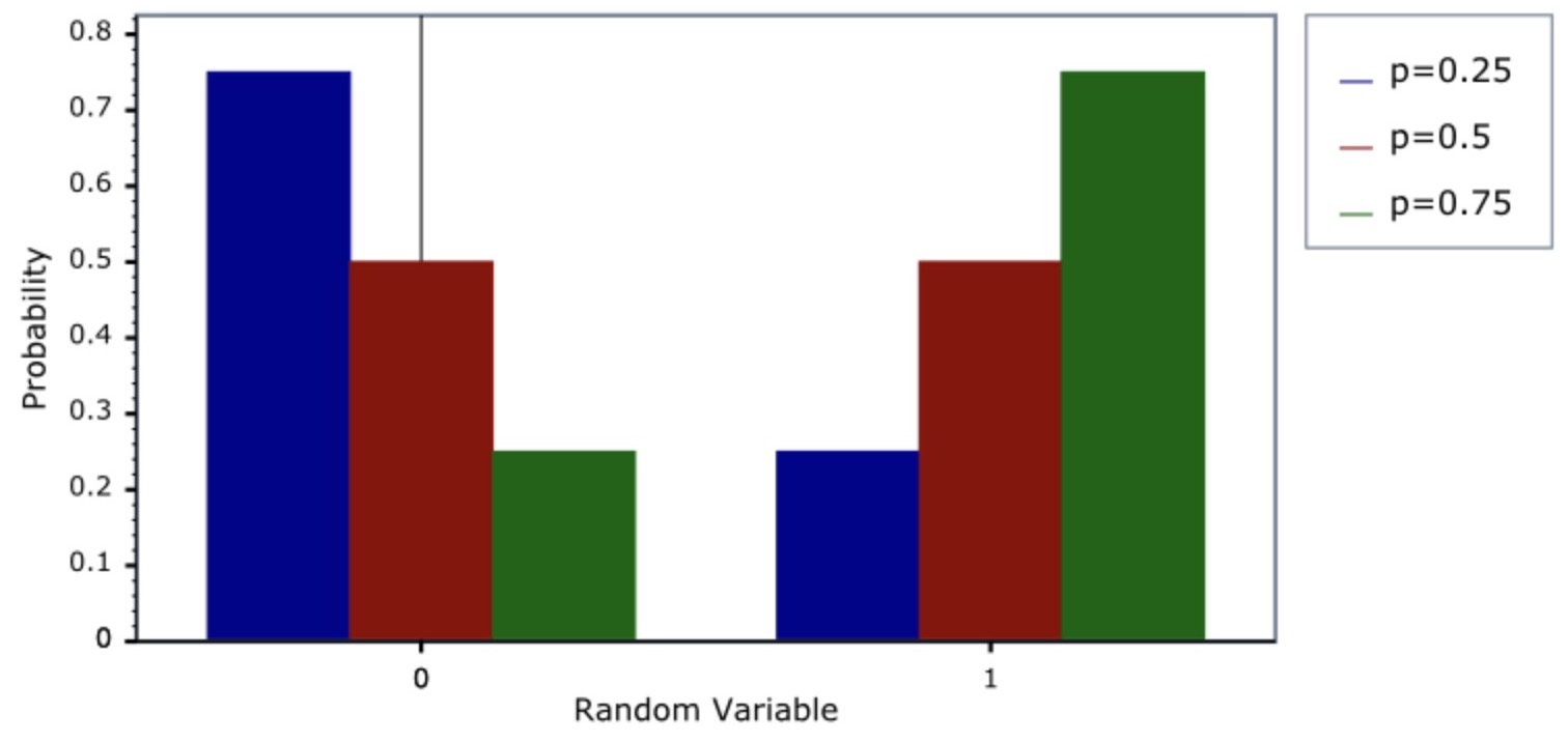
Bernoulli distribution
- The Bernoulli distribution arises as the result of a binary outcome, which is why it is used to model binary data.
- For e.g., building a spam vs. ham binary classifier, or modeling a coin toss.
- A Bernoulli random variable thus models a discrete distribution.
- Bernoulli random variables take the values 0 and 1 with probabilities of \(p\) and \(1-p\), respectively.
- The mean of a Bernoulli random variable is \(p\) and the variance is \(p(1 - p)\).
- If we let \(X\) be a Bernoulli random variable, it is typical to call \(X=1\) as a “success” and \(X=0\) as a “failure”.
PMF
- The probability mass function \(f(\cdot)\) of a Bernoulli distribution, over possible outcomes \(k \in \{0,1\}\), is given by,
- This can also be expressed as,
- or as,
- Note that the Bernoulli distribution is a special case of the binomial distribution with \(n=1\).
IID Bernoulli Trials
-
The Bernoulli distribution models the outcome of a single trial with two possible results: “success” (usually represented by 1) and “failure” (represented by 0). The probability of success is denoted by \(p\), while the probability of failure is \(1 - p\). When we perform multiple independent trials with the same probability of success, we can sum these outcomes to form a Binomial distribution.
-
If several IID (independent and identically distributed) Bernoulli trials \(x_1, x_2, \ldots, x_n\) are conducted, we can calculate the probability (likelihood) of observing a particular sequence of outcomes as:
\[\prod_{i=1}^n p^{x_i} (1 - p)^{1 - x_i} = p^{\sum x_i} (1 - p)^{n - \sum x_i}\] -
This likelihood depends only on the sum of the observed outcomes, \(\sum x_i\), rather than on the individual trials themselves. Consequently, the sample proportion \(\frac{\sum x_i}{n}\) contains all the relevant information about \(p\), the probability of success in each trial.
-
By maximizing the likelihood with respect to \(p\), we obtain the maximum likelihood estimator \(\hat{p}\) for the probability of success as:
\[\hat{p} = \frac{\sum_i x_i}{n}\]
Relationship between Binomial and Bernoulli distributions
- The Binomial and Bernoulli distributions are fundamentally connected, with the Binomial distribution serving as a generalization of the Bernoulli distribution. A Bernoulli distribution models a single trial with only two possible outcomes: “success” (represented by 1) and “failure” (represented by 0), where the probability of success is \(p\). However, when we extend this concept to multiple independent trials, each with the same probability of success, the result is a Binomial distribution.
- More formally, if we conduct \(n\) independent and identically distributed (IID) Bernoulli trials, represented by random variables \(X_1, X_2, \ldots, X_n\), each with success probability \(p\), then the sum \(X = \sum_{i=1}^n X_i\) follows a Binomial distribution with parameters \(n\) (the number of trials) and \(p\) (the probability of success in each trial). The Binomial probability mass function (PMF) for obtaining exactly \(x\) successes out of \(n\) trials is given by:
- In this way, the Bernoulli distribution is a special case of the Binomial distribution where the number of trials \(n = 1\). When \(n = 1\), the Binomial distribution simplifies to a Bernoulli distribution with parameter \(p\), modeling a single binary outcome rather than the count of successes over multiple trials.
- Thus, the Binomial distribution generalizes the Bernoulli distribution to scenarios with multiple trials, with the Bernoulli distribution effectively being a Binomial distribution limited to a single trial.
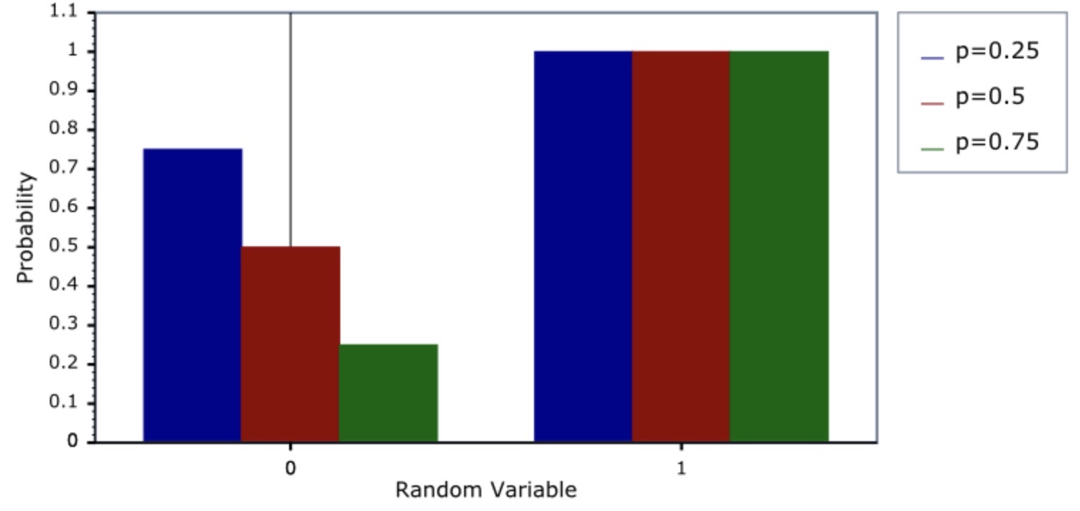
CDF
- The cumulative density function (CDF) of the Bernoulli distribution is given by,
Binomial Distribution
- A binomial distribution models the probability of obtaining a specific number of “successes” in a fixed number of independent trials, where each trial has only two possible outcomes: “success” or “failure.”
- Importantly, the binomial distribution always ranges between 0 and 1 because it represents probabilities. Here, a probability of 0 indicates an impossible event, while a probability of 1 represents a certain event.
- In the binomial distribution, each trial has a probability \(p\) of success and \(1 - p\) of failure. The entire distribution, which captures the probabilities of obtaining different numbers of successes across trials, must fall within this range due to these probabilities.
Binomial Trials
- Binomial random variables result from the sum of independent and identically distributed (IID) Bernoulli trials. If \(X_1, X_2, \ldots, X_n\) are IID Bernoulli trials with probability \(p\) of success, the sum \(X = \sum_{i=1}^n X_i\) is a binomial random variable.
-
The probability mass function (PMF) of a binomial random variable is:
\[P(X = x) = \binom{n}{x} p^x (1 - p)^{n - x} \quad \text{for } x = 0, \ldots, n\]- where \(\binom{n}{x}\) represents the number of ways to achieve \(x\) successes out of \(n\) trials.
The selection problem
- The notation \(^nC_{x}\) or \({n \choose x} = \frac{n!}{x!(n-x)!}\) (read “\(n\) choose \(x\)”) counts the number of ways of selecting \(x\) items out of \(n\) without replacement disregarding the order of the items.
- Also,
Example justification of the binomial likelihood
- Consider the probability of getting 6 heads out of 10 coin flips from a coin with success probability \(p\).
- The probability of getting 6 heads and 4 tails in any specific order is \(p^6(1-p)^4\).
- There are \({10 \choose 6}\) possible orders of 6 heads and 4 tails.
Example
- Suppose a friend has 8 children, 7 of which are girls and none are twins.
- If each gender has an independent 50% probability for each birth, what’s the probability of getting 7 or more girls out of 8 births?
choose(8, 7) * 0.5 ^ 8 + choose(8, 8) * 0.5 ^ 8 # Returns 0.03516
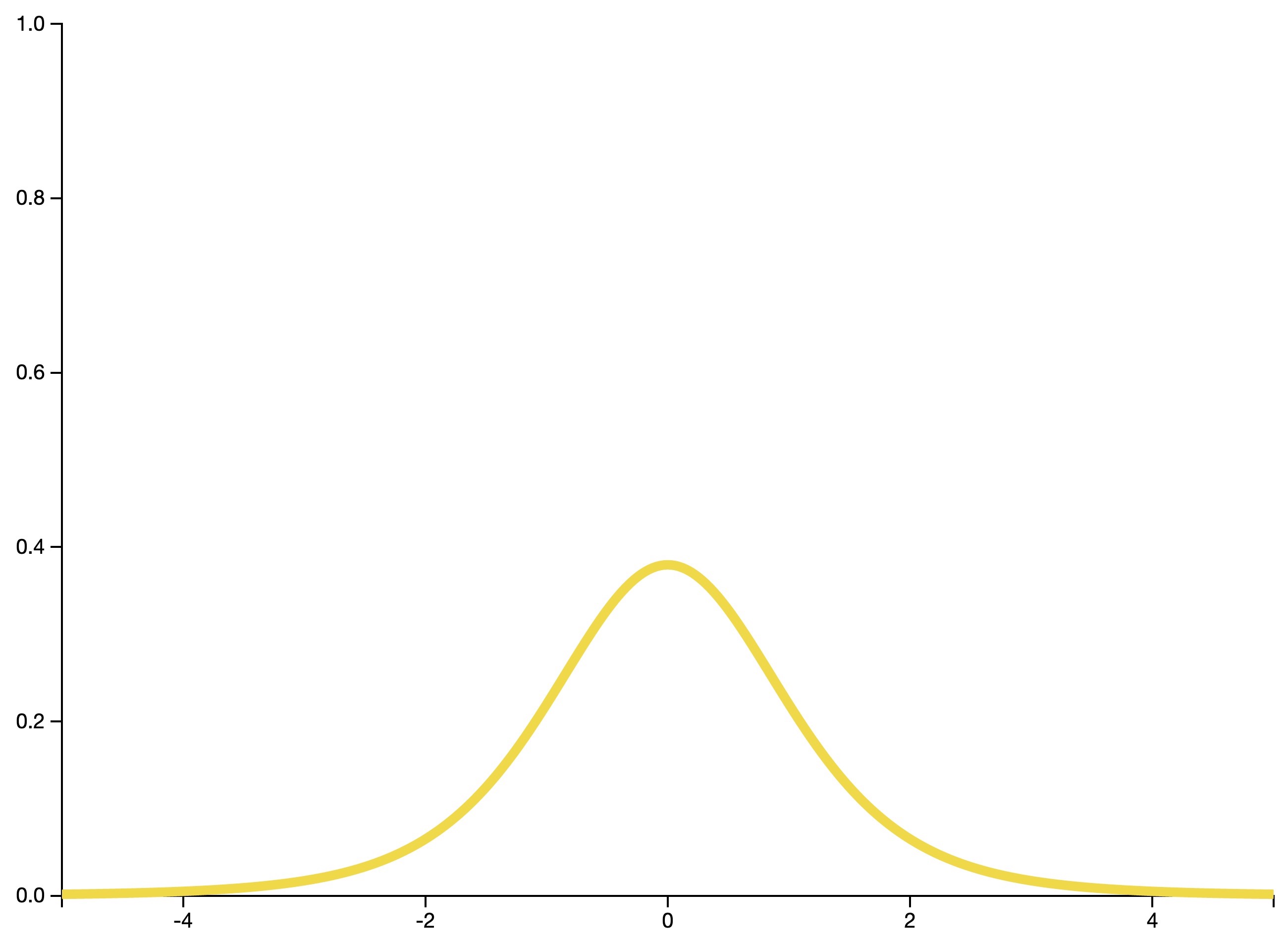
Gaussian/normal distribution
- The normal (or Gaussian) distribution has a bell-shaped density function and is used to model real-valued random variables that are assumed to be additively produced by many small effects.
- For example, the normal distribution is used to model people’s height, since height can be assumed to be the result of many small genetic and evironmental factors.
- Another example would be modeling the price of a house, since the price of a house can be assumed to be a function of the area, school district, distance to landmarks etc.
- If \(X\) a random variable the follows a Gaussian distribution then, \(E[X] = \mu\) and \(Var(X) = \sigma^2\).
- The notation used to indicate that a random variable was sampled from a normal distribution is: \(X\sim \mathcal{N}(\mu, \sigma^2)\).
- A random variable is said to follow a normal or Gaussian distribution with mean \(\mu\) and variance \(\sigma^2\) if the associated PDF is,

CDF
-
The CDF of the Gaussian distribution is given by,
\[F(x)=\Phi\left(\frac{x-\mu}{\sigma}\right)=\frac{1}{2}\left[1+\operatorname{erf}\left(\frac{x-\mu}{\sigma \sqrt{2}}\right)\right]\]- where,
- \(\Phi(\cdot)\) represents the CDF of the standard normal distribution.
- \(\operatorname {erf} (x)\) represents the error function.
- where,

Standard normal distribution
- The simplest case of a the normal distribution is called the standard normal distribution. This is a special case when \(\mu = 0\) and \(\sigma = 1\), described by the PDF:
- Note that the standard normal density function is denoted by \(\phi\).
- Standard normal random variables are often labeled \(Z\).
Example 1
- What is the \(95^{th}\) percentile of a \(\mathcal{N}(\mu, \sigma^2)\) distribution?
- We want the point \(x_0\) so that \(P(X \leq x_0) = 0.95\).
- \(\therefore\) \(\frac{x_0 - \mu}{\sigma} = 1.645\) or \(x_0 = \mu + \sigma 1.645\).
- In general, \(x_0 = \mu + \sigma z_0\) where \(z_0\) is the appropriate standard normal quantile.
Example 2
- What is the probability that a \(\mathcal{N}(\mu,\sigma^2)\) random variable is \(2 \sigma\) (i.e., 2 standard deviations) above the mean?
- Formally, we can write the question as:
- This simplifies to,
Facts about the normal density
- If \(X \sim \mathcal{N}(\mu,\sigma^2)\), then \(Z = \frac{X -\mu}{\sigma}\) is the standard normal distribution.
- If \(Z \sim \phi\), i.e., Z is a random variable that follows the standard normal distribution, then \(X = \mu + \sigma Z \sim \mathcal{N}(\mu, \sigma^2)\).
- The PDF of a general normal distribution in terms of the PDF of a standard normal \(\phi(\cdot)\) is,
- Approximately \(68\%\), \(95\%\) and \(99.7\%\) of the normal density lies within 1, 2 and 3 standard deviations from the mean, respectively. \(-1.28\), \(-1.645\), \(-1.96\) and \(-2.33\) are the \(10^{th}\), \(5^{th}\), \(2.5^{th}\) and \(1^{st}\) percentiles of the standard normal distribution respectively.
- By symmetry, \(1.28\), \(1.645\), \(1.96\) and \(2.33\) are the \(90^{th}\), \(95^{th}\), \(97.5^{th}\) and \(99^{th}\) percentiles of the standard normal distribution respectively.
Other properties
- The normal distribution is symmetric and peaked around its mean (therefore the mean, median and mode are all equal).
- A constant times a normally distributed random variable is also normally distributed (what is the mean and variance?).
- Sums of normally distributed random variables are again normally distributed even if the variables are dependent (what is the mean and variance?).
- Sample means of normally distributed random variables are again normally distributed (with what mean and variance?).
- The square of a standard normal random variable follows what is called chi-squared distribution.
- The exponent of a normally distributed random variables follows what is called the log-normal distribution.
- As we will see later, many random variables, properly normalized, limit to a normal distribution.
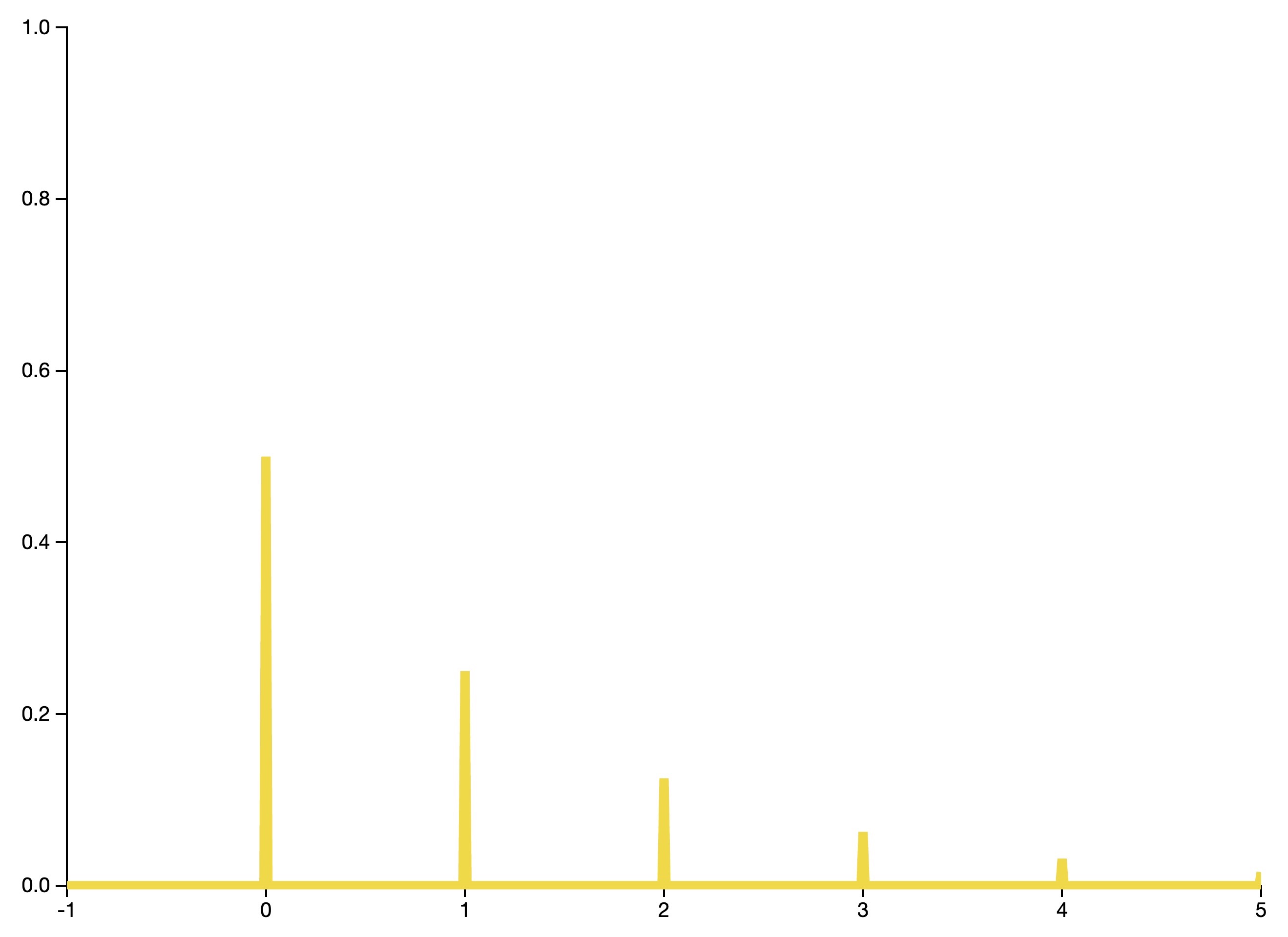
Poisson distribution
- A Poisson random variable counts the number of events occurring in a fixed interval of time or space, given that these events occur with an average rate \(\lambda\).
- This distribution can be used to model events such as:
- The number of meteor showers in a year.
- The number of goals in a soccer match.
- The number of patients arriving in an emergency room between 10 and 11 PM.
- The number of laser photons hitting a detector in a particular time interval.
- The number of customers arriving in a store (or say, the number of page-views on a website).
- A Poisson random variable thus models a discrete distribution.
- Both the mean and variance of this distribution is \(\lambda\).
- Note that \(\lambda\) ranges from 0 to \(\infty\).
PMF
- The PMF of the the Poisson distribution is given by,

CDF
- The CDF of the Poisson distribution is given by,

Use-cases for the Poisson distribution
- Modeling count data, i.e., data of the form \(\frac{\text{number of events}}{\text{time}}\). Examples include radioactive decay, survival data, contingency tables etc.
- Approximating binomials when \(n\) is large and \(p\) is small.
Poisson derivation
- Let \(h\) be very small.
- Now, if we assume that…
- Prob. of an event in an interval of length \(h\) is \(\lambda h\) while the prob. of more than one event is negligible.
- Whether or not an event occurs in one small interval does not impact whether or not an event occurs in another small interval
- … then, the number of events per unit time is Poisson with mean \(\lambda\).
Rates and Poisson random variables
- Poisson random variables are used to model rates.
- \(X \sim \operatorname{Poisson}(\lambda t)\) where,
- \(\lambda = E\left[\frac{X}{t}\right]\) is the expected count per unit of time.
- \(t\) is the total monitoring time.
Poisson approximation to the binomial
- A binomial random variable is the sum of \(n\) independent Bernoulli random variables with parameter \(p\). It is frequently used to model the number of successes in a specified number of identical binary experiments, such as the number of heads in five coin tosses.
- When \(n\) is large and \(p\) is small (with \(np < 10\)), the Poisson distribution is an accurate approximation to the binomial distribution.
- Formally, \(X \sim \mbox{Binomial}(n, p)\), \(\lambda = n p\).
Example
- The number of people that show up at a bus stop is Poisson with a mean of \(2.5\) per hour.
- If watching the bus stop for 4 hours, what is the probability that 3 or fewer people show up for the whole time?
ppois(3, lambda = 2.5 * 4) # Returns 0.01034
Example: Poisson approximation to the binomial
- If we flip a coin with success probablity \(0.01\) five hundred times, what’s the probability of 2 or fewer successes?
pbinom(2, size=500, prob=0.01) # Returns 0.1234
ppois(2, lambda=500 * 0.01) # Returns 0.1247
Uniform distribution
- The uniform distribution (or rectangular distribution) is a continuous distribution such that all intervals of equal length on the distribution’s support have equal probability. For example, this distribution might be used to model people’s full birth dates, where it is assumed that all times in the calendar year are equally likely.
- The distribution describes an experiment where there is an arbitrary outcome that lies between certain bounds.
- The bounds are defined by the parameters, \(a\) and \(b\), which are the minimum and maximum values. The interval can be either be closed (e.g., \([a, b]\)) or open (e.g., \((a, b)\)).
- Therefore, the distribution is often abbreviated \(U(a, b)\), where \(U\) stands for uniform distribution.
- The PDF of the continuous uniform distribution is given by,

CDF
- The CDF of the continuous uniform distribution is given by,

Geometric distribution
- A geometric random variable counts the number of trials that are required to observe a single success, where each trial is independent and has success probability \(p\). A geometric random variable thus models a discrete distribution.
- For example, this distribution can be used to model the number of times a die must be rolled in order for a six to be observed.
Student’s t-distribution
- A Student’s t-distribution (or simply the t-distribution), is a continuous probability distribution that arises when estimating the mean of a normally distributed population in situations where the sample size is small and population standard deviation is unknown.
Chi-squared distribution
- A chi-squared random variable with \(k\) degrees of freedom is the sum of \(k\) independent and identically distributed squared standard normal random variables. A chi-squared random variable thus models a continuous distribution.
- It is often used in hypothesis testing and in the construction of confidence intervals.
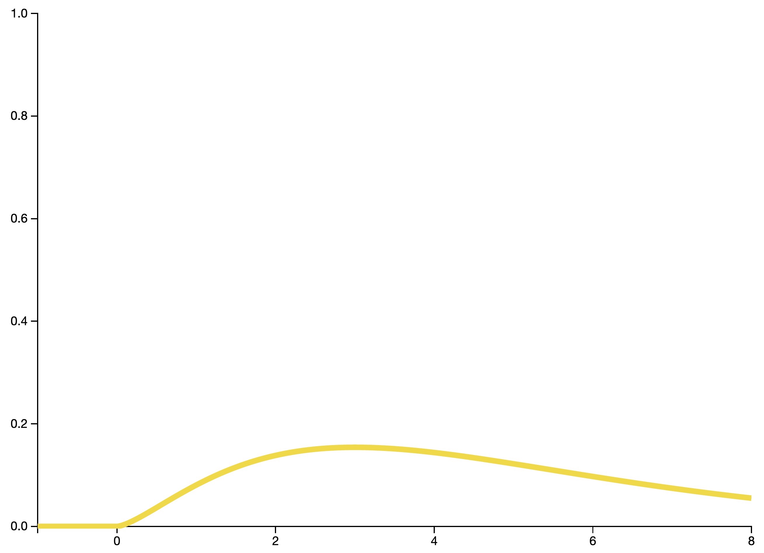
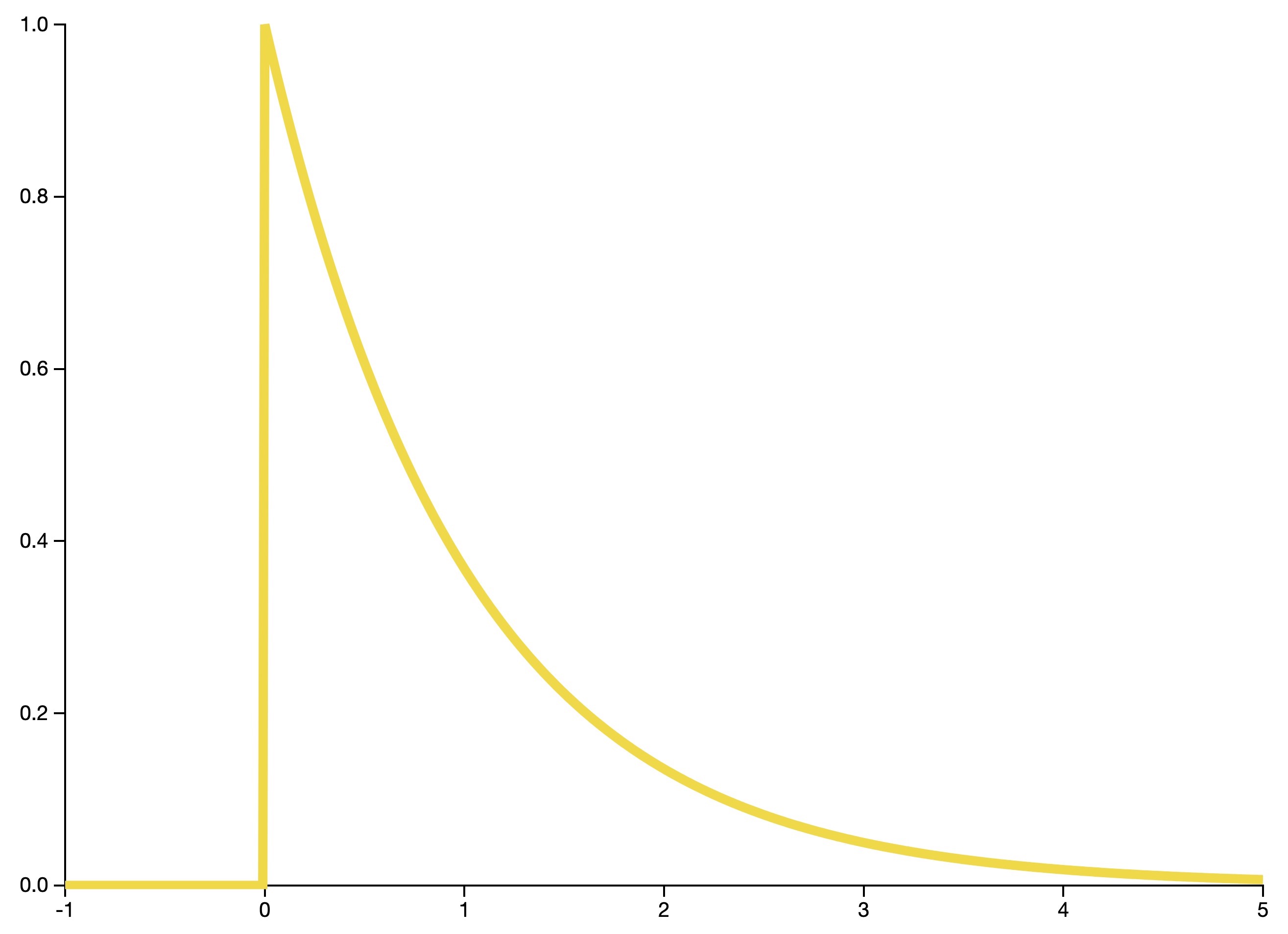
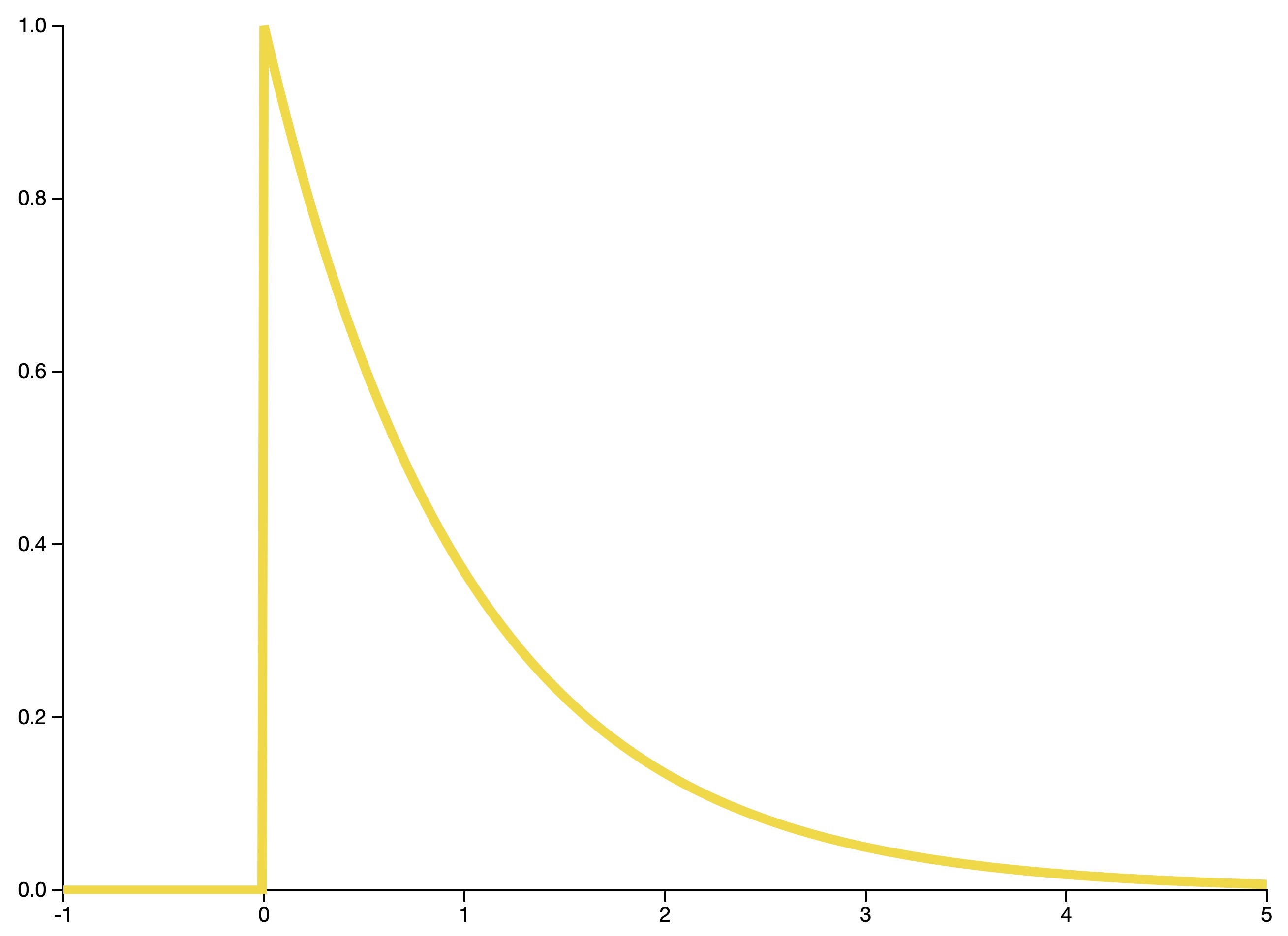
Exponential distribution
- The exponential distribution is the continuous analogue of the geometric distribution. It is often used to model waiting times.
F distribution
- The F-distribution (also known as the Fisher–Snedecor distribution), is a continuous distribution that arises frequently as the null distribution of a test statistic, most notably in the analysis of variance.
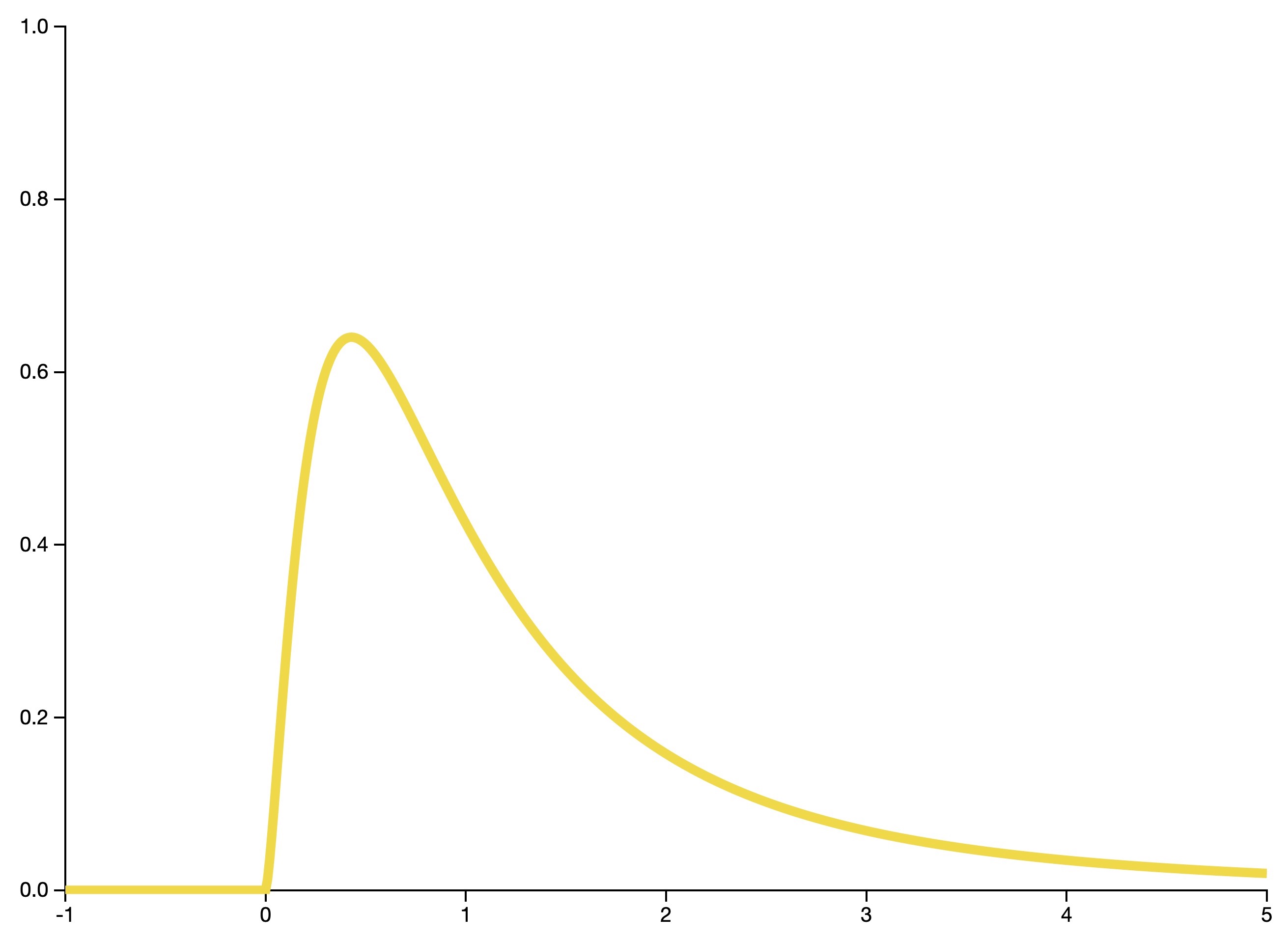
Gamma distribution
- The gamma distribution is a general family of continuous probability distributions. The exponential and chi-squared distributions are special cases of the gamma distribution.
Beta distribution
- The beta distribution is a general family of continuous probability distributions bound between 0 and 1. The beta distribution is frequently used as a conjugate prior distribution in Bayesian statistics.
Frequentist inference
- Frequentist inference is the process of determining properties of an underlying distribution via the observation of data.
Point estimation
- One of the main goals of statistics is to estimate unknown parameters. To approximate these parameters, we choose an estimator, which is simply any function of randomly sampled observations. To illustrate this idea, let’s consider the problem of estimating the value of \(\pi\). To do so, we can uniformly drop samples on a square containing an inscribed circle. Notice that the value of \(\pi\) can be expressed as a ratio of the areas,
- We can estimate this ratio with our samples. Let \(m\) be the number of samples within our circle and \(n\) the total number of samples dropped. We define our estimator \(\hat{\pi}\) as:
- It can be shown that this estimator has the desirable properties of being unbiased and consistent.
Confidence intervals
- In contrast to point estimators, confidence intervals estimate a parameter by specifying a range of possible values. Such an interval is associated with a confidence level, which is the probability that the procedure used to generate the interval will produce an interval containing the true parameter.
The Bootstrap
- Much of frequentist inference centers on the use of “good” estimators. The precise distributions of these estimators, however, can often be difficult to derive analytically. The computational technique known as the Bootstrap provides a convenient way to estimate properties of an estimator via resampling.
Bayesian inference
- Bayesian inference techniques specify how one should update one’s beliefs upon observing data.
Bayes’ Theorem
- Suppose that on your most recent visit to the doctor’s office, you decide to get tested for a rare disease. If you are unlucky enough to receive a positive result, the logical next question is, “Given the test result, what is the probability that I actually have this disease?” (Medical tests are, after all, not perfectly accurate.) Bayes’ Theorem tells us exactly how to compute this probability:
- As the equation indicates, the posterior probability of having the disease given that the test was positive depends on the prior probability of the disease \(P(Disease)\). Think of this as the incidence of the disease in the general population. Set this probability by dragging the bars below.
- The posterior probability also depends on the test accuracy: How often does the test correctly report a negative result for a healthy patient, and how often does it report a positive result for someone with the disease?
Likelihood Function
- In statistics, the likelihood function has a very precise definition:
- The concept of likelihood plays a fundamental role in both Bayesian and frequentist statistics. To read more, refer the section on likelihood vs. probability in our CS229 notes.
Prior to Posterior
- At the core of Bayesian statistics is the idea that prior beliefs should be updated as new data is acquired. Consider a possibly biased coin that comes up heads with probability \(p\). This purple slider determines the value of \(p\) (which would be unknown in practice).
- As we acquire data in the form of coin tosses, we update the posterior distribution on \(p\), which represents our best guess about the likely values for the bias of the coin. This updated distribution then serves as the prior for future coin tosses.
Regression Analysis
- Linear regression is an approach for modeling the linear relationship between two variables.
Ordinary Least Squares
- The ordinary least squares (OLS) approach to regression allows us to estimate the parameters of a linear model.
- The goal of this method is to determine the linear model that minimizes the sum of the squared errors between the observations in a dataset and those predicted by the model.
Correlation
- Correlation is a measure of the linear relationship between two variables. It is defined for a sample as the following and takes value between +1 and -1 inclusive:
- \(s_{x y}, s_{x x}, s_{y y}\) are defined as:
- It can also be understood as the cosine of the angle formed by the ordinary least square line determined in both variable dimensions.
Analysis of Variance
- Analysis of Variance (ANOVA) is a statistical method for testing whether groups of data have the same mean. ANOVA generalizes the t-test to two or more groups by comparing the sum of square error within and between groups.
Trigonometry
Ratios
| \(Angle^{\circ}\) | \(0^{\circ}\) | \(30^{\circ}\) | \(45^{\circ}\) | \(60^{\circ}\) | \(90^{\circ}\) |
|---|---|---|---|---|---|
| \(Angle^{c}\) | \(0^{c}\) | \({\pi/6}^{c}\) | \({\pi/4}^{c}\) | \({\pi/3}^{c}\) | \({\pi/2}^{c}\) |
| \(\sin \theta\) | 0 | \(\frac{1}{2}\) | \(\frac{1}{\sqrt{2}}\) | \(\frac{\sqrt{3}}{2}\) | 1 |
| \(\cos \theta\) | 1 | \(\frac{\sqrt{3}}{2}\) | \(\frac{1}{\sqrt{2}}\) | \(\frac{1}{2}\) | 0 |
| \(\tan \theta\) | 0 | \(\frac{1}{\sqrt{3}}\) | 1 | \(\sqrt{3}\) | \(\text{N/A}\) |
| \(\operatorname{cosec} \theta\) | \(\text{N/A}\) | 2 | \(\sqrt{2}\) | \(\frac{2}{\sqrt{3}}\) | 1 |
| \(\sec \theta\) | 1 | \(\frac{2}{\sqrt{3}}\) | \(\sqrt{2}\) | 2 | \(\text{N/A}\) |
| \(\cot \theta\) | \(\text{N/A}\) | \(\sqrt{3}\) | 1 | \(\frac{1}{\sqrt{3}}\) | 0 |
- \(\text{N/A}\) = not defined.
Graphical view of sin and cos
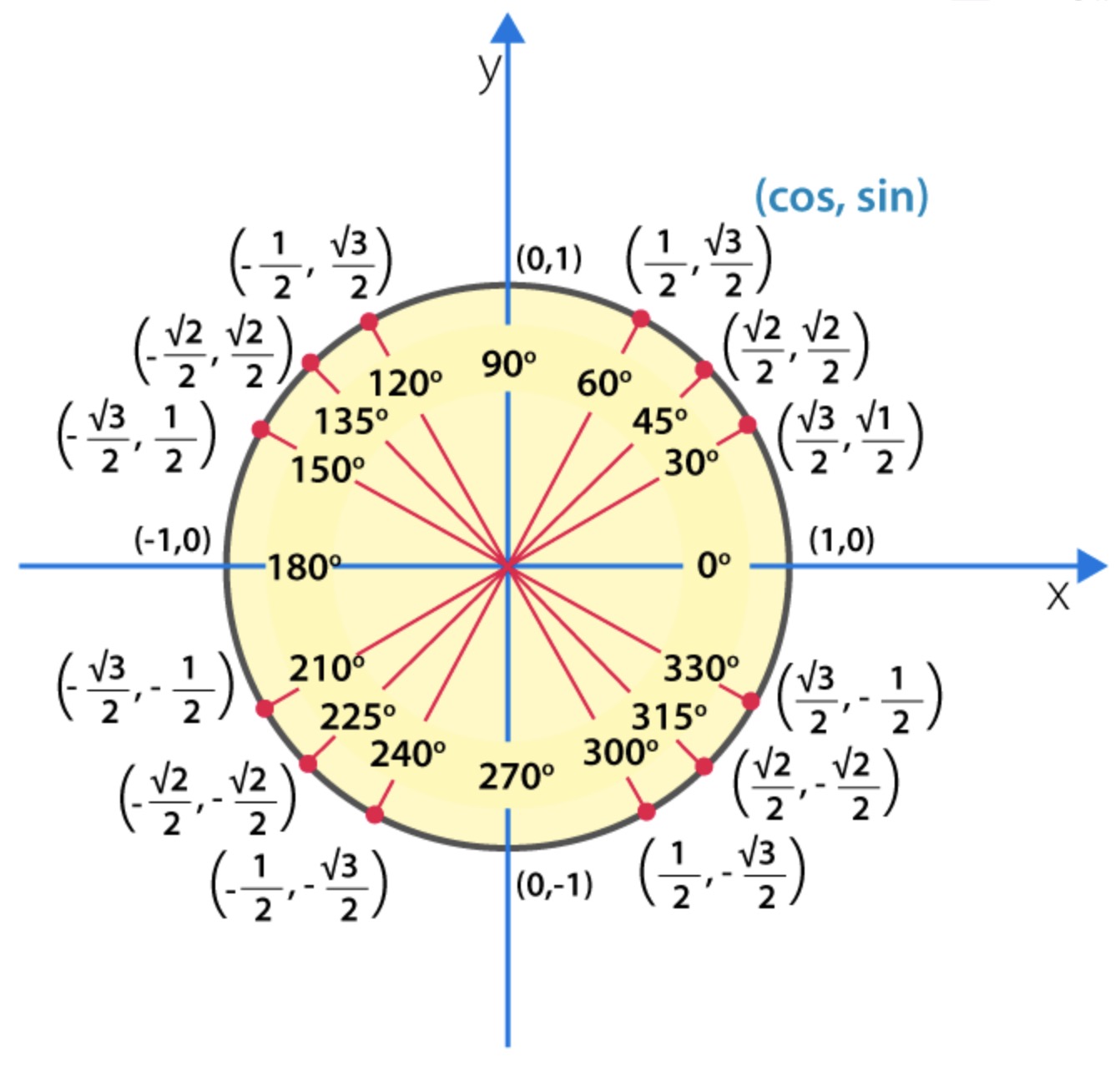
- Shown below is a graphical view of how \(\cos (\theta)\) and \(\sin (\theta)\) vary as the angle goes from \(0^{\circ}\) to \(360^{\circ}\) (or equivalently, \(0^{c}\) to \(2\pi^{c}\)).
- Note that the below diagram shows a unit circle (with radius = 1).
References and Credits
- Aurélien Geron’s Hands-on Machine Learning with Scikit-Learn, Keras and TensorFlow served as a major inspiration for this tutorial.
- Seeing Theory helped with sections that offer an overview to probability and statistics.
- 5 Derivatives to Excel in Your Machine Learning Interview helped with examples on derivatives for uni- and multi-dimensional functions, including the gradient, Jacobian and Hessian.
- Wikipedia articles on Bernoulli distribution, Normal distribution, Poisson distribution and Uniform distribution.
- Wolfram MathWorld article on Bernoulli distribution.
- Trigonometric functions for a graphical view into how \(\cos (\theta)\) and \(\sin (\theta)\) vary with \(\theta\).
Citation
If you found our work useful, please cite it as:
@article{Chadha2020DistilledMathTutorial,
  title   = {Math Tutorial},
  author  = {Chadha, Aman},
  journal = {Distilled AI},
  year    = {2020},
  note    = {\url{https://aman.ai}}
}