Primers • Pandas
- Overview
- Background
- Prerequisites
- Setup
- Overview: pandas data-structures
- Pandas is column-major
- Series objects
- DataFrame objects
- Creating a DataFrame
- Multi-indexing
- Dropping a level
- Transposing
- Stacking and unstacking levels
- Accessing rows
- Accessing columns
- Adding and removing columns
- Evaluating an expression
- Querying a DataFrame
- Sorting a DataFrame
- Plotting a DataFrame
- Operations on DataFrames
- Automatic alignment
- Handling missing data
- Aggregating using
groupby - Get the N Largest Values for Each Category in a DataFrame
- Assign Name to a Pandas Aggregation
pd.pivot_table(): Turn Your DataFrame Into a Pivot Table- Overview functions
- Saving and loading
- Combining DataFrames
- Categories
- Practical example using a sample dataset
- Selected Methods
- Creating a DataFrame
- Transforming/Modifying a DataFrame
Series.map(): Change Values of a Pandas Series Using a DictionaryDataFrame.to_frame(): Convert Series to DataFrameDataFrame.values: Return a NumPy representation of the DataFrameDataFrame.apply(): Apply a Function to a Column of a DataFrameDataFrame.assign(): Assign Values to Multiple New ColumnsDataFrame.groupby(): Group DataFrame using a mapper or by a Series of columnsDataFrame.explode(): Transform Each Element in an Iterable to a RowDataFrame.fillna(method="ffill"): Forward Fill in pandaspd.melt(): Unpivot a DataFramepd.crosstab(): Create a Cross Tabulationpd.DataFrame.agg(): Aggregate over Columns or Rows Using Multiple Operationspd.DataFrame.agg(): Apply Different Aggregations to Different Columns
- Analyzing a DataFrame
- What’s next?
- References and Credits
- Citation

Overview
- The pandas library provides high-performance, easy-to-use data structures and data analysis tools. The main data structure is the DataFrame, which you can think of as an in-memory 2D table (like a spreadsheet, with column names and row labels).
- Many features available in Excel are available programmatically, such as creating pivot tables, computing columns based on other columns, plotting graphs, etc. You can also group rows by column value, or join tables much like in SQL. Pandas is also great at handling time series data.
Background
- It’s possible that Python wouldn’t have become the lingua franca of data science if it wasn’t for pandas.
- This tutorial contains a few peculiar things about pandas that hopefully make your life easier and code faster.
Prerequisites
- If you are not familiar with NumPy, we recommend that you go through the NumPy tutorial now.
Setup
- First, let’s import pandas. People usually import it as
pd:
import pandas as pd
Overview: pandas data-structures
- The pandas library contains these useful data structures:
- Series objects: A Series object is 1D array, similar to a column in a spreadsheet (with a column name and row labels).
- DataFrame objects: A DataFrame is a concept inspired by R’s Data Frame, which is, in turn, similar to tables in relational databases. This is a 2D table with rows and columns, similar to a spreadsheet (with names for columns and labels for rows).
- Panel objects: You can see a Panel as a dictionary of DataFrames. These are less used, so we will not discuss them here.
Pandas is column-major
An important thing to know about pandas is that it is column-major, which explains many of its quirks.
- Column-major means consecutive elements in a column are stored next to each other in memory. Row-major means the same but for elements in a row. Because modern computers process sequential data more efficiently than non-sequential data, if a table is row-major, accessing its rows will be much faster than accessing its columns.
- In NumPy, major order can be specified. When a
ndarrayis created, it’s row-major by default if you don’t specify the order. - Like R’s Data Frame, pandas’ DataFrame is column-major. People coming to pandas from NumPy tend to treat DataFrame the way they would
ndarray, e.g. trying to access data by rows, and find DataFrame slow. - Note: A column in a DataFrame is a Series. You can think of a DataFrame as a bunch of Series being stored next to each other in memory.
- For our dataset, accessing a row takes about 50x longer than accessing a column in our DataFrame.
-
Run the following code snippet in a Colab/Jupyter notebook:
# Get the column `date`, 1000 loops %timeit -n1000 df["Date"] # Get the first row, 1000 loops %timeit -n1000 df.iloc[0]- which outputs:
  1.78 µs ± 167 ns per loop (mean ± std. dev. of 7 runs, 1000 loops each)
  145 µs ± 9.41 µs per loop (mean ± std. dev. of 7 runs, 1000 loops each)
Converting DataFrame to row-major order
-
If you need to do a lot of row operations, you might want to convert your DataFrame to a NumPy’s row-major
ndarray, then iterating through the rows. Run the following code snippet in a Colab/Jupyter notebook:# Now, iterating through our DataFrame is 100x faster. %timeit -n1 df_np = df.to_numpy(); rows = [row for row in df_np]- which outputs:
4.55 ms ± 280 µs per loop (mean ± std. dev. of 7 runs, 1 loop each) -
Accessing a row or a column of our
ndarraytakes nanoseconds instead of microseconds. Run the following code snippet in a Colab/Jupyter notebook:df_np = df.to_numpy() %timeit -n1000 df_np[0] %timeit -n1000 df_np[:,0]- which outputs:
  147 ns ± 1.54 ns per loop (mean ± std. dev. of 7 runs, 1000 loops each)
  204 ns ± 0.678 ns per loop (mean ± std. dev. of 7 runs, 1000 loops each)
Series objects
Creating a Series
-
Let’s start by creating our first Series object!
import pandas as pd pd.Series([1, 2, 3])- which outputs:
  0    1
  1    2
  2    3
  dtype: int64
Similar to a 1D ndarray
-
Series objects behave much like one-dimensional NumPy
ndarrays, and you can often pass them as parameters to NumPy functions:import pandas as pd s = pd.Series([1, 2, 3]) np.exp(s)- which outputs:
0 2.718282 1 7.389056 2 20.085537 dtype: float64 -
Arithmetic operations on Series are also possible, and they apply elementwise, just like for
ndarrays:s = pd.Series([1, 2, 3]) np.exp(s) s + [1000, 2000, 3000]- which outputs:
0 1001 1 2002 2 3003 dtype: int64 -
Similar to NumPy, if you add a single number to a Series, that number is added to all items in the Series. This is called broadcasting:
s = pd.Series([1, 2, 3]) np.exp(s) s + 1000- which outputs:
0 1001 1 1002 2 1003 dtype: int64 -
The same is true for all binary operations such as
*or/, and even conditional operations:s = pd.Series([1, 2, 3]) np.exp(s) s < 0- which outputs:
  0    False
  1    False
  2    False
  dtype: bool
Index labels
-
Each item in a Series object has a unique identifier called the index label. By default, it is simply the rank of the item in the Series (starting at
0) but you can also set the index labels manually:import pandas as pd s = pd.Series([68, 83, 112, 68], index=["alice", "bob", "charles", "darwin"]) s- which outputs:
alice 68 bob 83 charles 112 darwin 68 dtype: int64 -
You can then use the Series just like a
dict:s["bob"]- which outputs:
83 -
You can still access the items by integer location, like in a regular array:
s[1]- which outputs:
83 -
To make it clear when you are accessing by label, it is recommended to always use the
locattribute when accessing by label:s.loc["bob"]- which outputs:
83 -
Similarly, to make it clear when you are accessing by integer location, it is recommended to always use the
ilocattribute when accessing by integer location:s2.iloc[1]- which outputs:
83 -
Slicing a Series also slices the index labels:
s.iloc[1:3]- which outputs:
bob 83 charles 112 dtype: int64 -
Pitfall: This can lead to unexpected results when using the default numeric labels, so be careful:
surprise = pd.Series([1000, 1001, 1002, 1003]) surprise- which outputs:
  0    1000
  1    1001
  2    1002
  3    1003
  dtype: int64
surprise_slice = surprise[2:] surprise_slice- which outputs:
2 1002 3 1003 dtype: int64 -
Oh look! The first element has index label
2. The element with index label0is absent from the slice:try: surprise_slice[0] except KeyError as e: print("Key error:", e)- which outputs:
Key error: 0 -
But remember that you can access elements by integer location using the
ilocattribute. This illustrates another reason why it’s always better to uselocandilocto access Series objects:surprise_slice.iloc[0]- which outputs:
1002
Initialize using a dict
-
You can create a Series object from a
dict. The keys will be used as index labels:import pandas as pd weights = {"alice": 68, "bob": 83, "colin": 86, "darwin": 68} pd.Series(weights)- which outputs:
alice 68 bob 83 colin 86 darwin 68 dtype: int64 -
You can control which elements you want to include in the Series and in what order by explicitly specifying the desired
index:pd.Series(weights, index = ["colin", "alice"])- which outputs:
  colin    86
  alice    68
  dtype: int64
Automatic alignment
-
When an operation involves multiple Series objects, pandas automatically aligns items by matching index labels.
import pandas as pd s1 = pd.Series([68, 83, 112, 68], index=["alice", "bob", "charles", "darwin"]) weights = {"alice": 68, "bob": 83, "colin": 86, "darwin": 68} s2 = pd.Series(weights) print(s1.keys()) print(s2.keys()) s1 + s2- which outputs:
alice 136.0 bob 166.0 charles NaN colin NaN darwin 136.0 dtype: float64 - The resulting Series contains the union of index labels from
s2ands3. Since"colin"is missing froms2and"charles"is missing froms3, these items have aNaNresult value. (i.e., Not-a-Number means missing). -
Automatic alignment is very handy when working with data that may come from various sources with varying structure and missing items. But if you forget to set the right index labels, you can have surprising results:
s1 = pd.Series([68, 83, 112, 68], index=["alice", "bob", "charles", "darwin"]) s2 = pd.Series([1000, 1000, 1000, 1000]) print("s1 = ", s1.values) print("s2 = ", s2.values) s1 + s2- which outputs:
alice NaN bob NaN charles NaN darwin NaN 0 NaN 1 NaN 2 NaN 3 NaN dtype: float64 - Pandas could not align the Series, since their labels do not match at all, hence the full
NaNresult.
Initialize with a scalar
-
You can also initialize a Series object using a scalar and a list of index labels: all items will be set to the scalar.
pd.Series(42, ["life", "universe", "everything"])- which outputs:
  life          42
  universe      42
  everything    42
  dtype: int64
Series name
-
A Series can have a
name:pd.Series([83, 68], index=["bob", "alice"], name="weights")- which outputs:
  bob      83
  alice    68
  Name: weights, dtype: int64
Plotting a Series
- Pandas makes it easy to plot Series data using matplotlib (for more details on matplotlib, check out the matplotlib tutorial).
-
Just import matplotlib and call the
plot()method:%matplotlib inline import matplotlib.pyplot as plt temperatures = [4.4, 5.1, 6.1, 6.2, 6.1, 6.1, 5.7, 5.2, 4.7, 4.1, 3.9, 3.5] s = pd.Series(temperatures, name="Temperature") s.plot() plt.show()- which outputs:
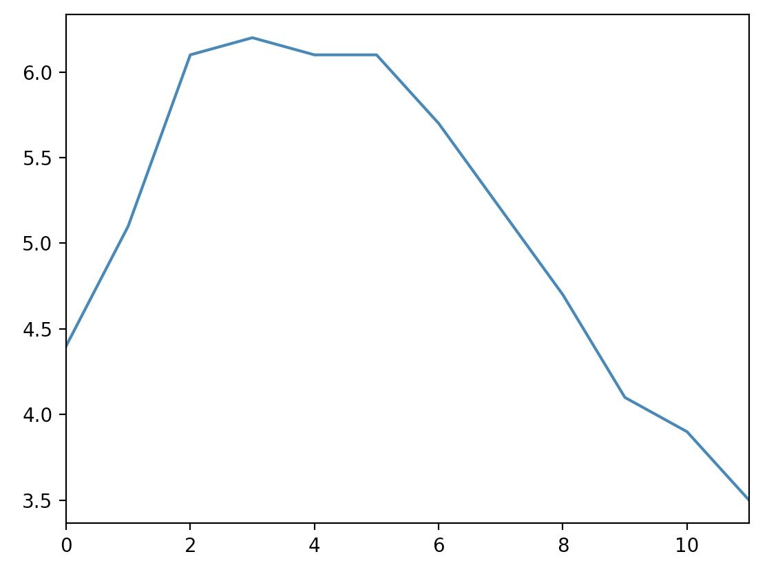
- There are many options for plotting your data. It is not necessary to list them all here: if you need a particular type of plot (histograms, pie charts, etc.), just look for it in the excellent visualization section of pandas’ documentation, and look at the example code.
Handling time
- Many datasets have timestamps, and pandas is awesome at manipulating such data:
- It can represent periods (such as 2016Q3) and frequencies (such as “monthly”),
- It can convert periods to actual timestamps, and vice versa,
- It can resample data and aggregate values any way you like,
- It can handle timezones.
Time range
-
Let’s start by creating a time series using
pd.date_range(). This returns aDatetimeIndexcontaining one datetime per hour for 12 hours starting on October 29th 2016 at 5:30PM.import pandas as pd dates = pd.date_range('2016/10/29 5:30pm', periods=12, freq='H') dates- which outputs:
DatetimeIndex(['2016-10-29 17:30:00', '2016-10-29 18:30:00', '2016-10-29 19:30:00', '2016-10-29 20:30:00', '2016-10-29 21:30:00', '2016-10-29 22:30:00', '2016-10-29 23:30:00', '2016-10-30 00:30:00', '2016-10-30 01:30:00', '2016-10-30 02:30:00', '2016-10-30 03:30:00', '2016-10-30 04:30:00'], dtype='datetime64[ns]', freq='H') -
This
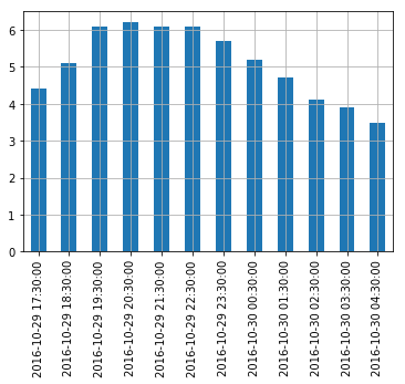
DatetimeIndexmay be used as an index in a Series:temperatures = [4.4, 5.1, 6.1, 6.2, 6.1, 6.1, 5.7, 5.2, 4.7, 4.1, 3.9, 3.5] temp_series = pd.Series(temperatures, dates) temp_series- which outputs:
2016-10-29 17:30:00 4.4 2016-10-29 18:30:00 5.1 2016-10-29 19:30:00 6.1 2016-10-29 20:30:00 6.2 2016-10-29 21:30:00 6.1 2016-10-29 22:30:00 6.1 2016-10-29 23:30:00 5.7 2016-10-30 00:30:00 5.2 2016-10-30 01:30:00 4.7 2016-10-30 02:30:00 4.1 2016-10-30 03:30:00 3.9 2016-10-30 04:30:00 3.5 Freq: H, dtype: float64 -
Let’s plot this series:
import matplotlib.pyplot as plt temp_series.plot(kind="bar") plt.grid(True) plt.show()- which outputs:
Resampling
-
Pandas lets us resample a time series very simply. Just call the
resample()method and specify a new frequency:import pandas as pd temp_series = pd.Series({pd.Timestamp('2016-10-29 17:30:00', freq='H'): 4.4, pd.Timestamp('2016-10-29 18:30:00', freq='H'): 5.1, pd.Timestamp('2016-10-29 19:30:00', freq='H'): 6.1, pd.Timestamp('2016-10-29 20:30:00', freq='H'): 6.2, pd.Timestamp('2016-10-29 21:30:00', freq='H'): 6.1, pd.Timestamp('2016-10-29 22:30:00', freq='H'): 6.1, pd.Timestamp('2016-10-29 23:30:00', freq='H'): 5.7, pd.Timestamp('2016-10-30 00:30:00', freq='H'): 5.2, pd.Timestamp('2016-10-30 01:30:00', freq='H'): 4.7, pd.Timestamp('2016-10-30 02:30:00', freq='H'): 4.1, pd.Timestamp('2016-10-30 03:30:00', freq='H'): 3.9, pd.Timestamp('2016-10-30 04:30:00', freq='H'): 3.5}) temp_series_freq_2H = temp_series.resample("2H") temp_series_freq_2H- which outputs:
<pandas.core.resample.DatetimeIndexResampler object at [address]> -
The resampling operation is actually a deferred operation, which is why we did not get a Series object, but a
DatetimeIndexResamplerobject instead. To actually perform the resampling operation, we can simply call themean()method: Pandas will compute the mean of every pair of consecutive hours:temp_series_freq_2H = temp_series_freq_2H.mean() temp_series_freq_2H- which outputs:
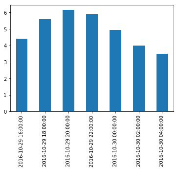
2016-10-29 16:00:00 4.40 2016-10-29 18:00:00 5.60 2016-10-29 20:00:00 6.15 2016-10-29 22:00:00 5.90 2016-10-30 00:00:00 4.95 2016-10-30 02:00:00 4.00 2016-10-30 04:00:00 3.50 Freq: 2H, dtype: float64 -
Let’s plot the result:
temp_series_freq_2H.plot(kind="bar") plt.show()- which outputs:
-
Note how the values have automatically been aggregated into 2-hour periods. If we look at the 6-8PM period, for example, we had a value of
5.1at 6:30PM, and6.1at 7:30PM. After resampling, we just have one value of5.6, which is the mean of5.1and6.1. Rather than computing the mean, we could have used any other aggregation function, for example we can decide to keep the minimum value of each period:temp_series_freq_2H = temp_series.resample("2H").min() temp_series_freq_2H- which outputs:
2016-10-29 16:00:00 4.4 2016-10-29 18:00:00 5.1 2016-10-29 20:00:00 6.1 2016-10-29 22:00:00 5.7 2016-10-30 00:00:00 4.7 2016-10-30 02:00:00 3.9 2016-10-30 04:00:00 3.5 Freq: 2H, dtype: float64 -
Or, equivalently, we could use the
apply()method instead:import numpy as np temp_series_freq_2H = temp_series.resample("2H").apply(np.min) temp_series_freq_2H- which outputs:
  2016-10-29 16:00:00    4.4
  2016-10-29 18:00:00    5.1
  2016-10-29 20:00:00    6.1
  2016-10-29 22:00:00    5.7
  2016-10-30 00:00:00    4.7
  2016-10-30 02:00:00    3.9
  2016-10-30 04:00:00    3.5
  Freq: 2H, dtype: float64
Upsampling and interpolation
-
The above was an example of downsampling. We can also upsample (i.e., increase the frequency), but this creates holes in our data:
import pandas as pd temp_series = pd.Series({pd.Timestamp('2016-10-29 17:30:00', freq='H'): 4.4, pd.Timestamp('2016-10-29 18:30:00', freq='H'): 5.1, pd.Timestamp('2016-10-29 19:30:00', freq='H'): 6.1, pd.Timestamp('2016-10-29 20:30:00', freq='H'): 6.2, pd.Timestamp('2016-10-29 21:30:00', freq='H'): 6.1, pd.Timestamp('2016-10-29 22:30:00', freq='H'): 6.1, pd.Timestamp('2016-10-29 23:30:00', freq='H'): 5.7, pd.Timestamp('2016-10-30 00:30:00', freq='H'): 5.2, pd.Timestamp('2016-10-30 01:30:00', freq='H'): 4.7, pd.Timestamp('2016-10-30 02:30:00', freq='H'): 4.1, pd.Timestamp('2016-10-30 03:30:00', freq='H'): 3.9, pd.Timestamp('2016-10-30 04:30:00', freq='H'): 3.5}) temp_series_freq_15min = temp_series.resample("15Min").mean() temp_series_freq_15min.head(n=10) # `head` displays the top n values- which outputs:
2016-10-29 17:30:00 4.4 2016-10-29 17:45:00 NaN 2016-10-29 18:00:00 NaN 2016-10-29 18:15:00 NaN 2016-10-29 18:30:00 5.1 2016-10-29 18:45:00 NaN 2016-10-29 19:00:00 NaN 2016-10-29 19:15:00 NaN 2016-10-29 19:30:00 6.1 2016-10-29 19:45:00 NaN Freq: 15T, dtype: float64 -
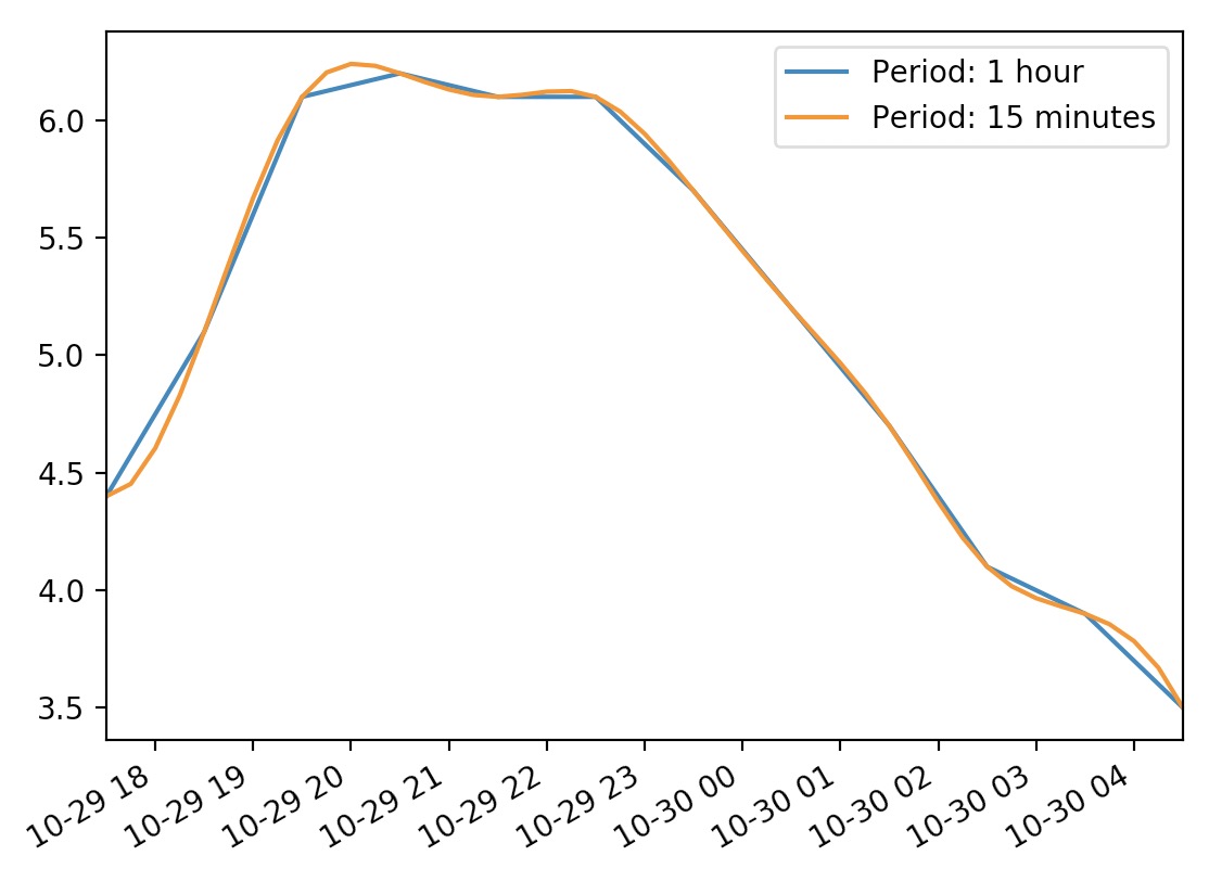
One solution is to fill the gaps by interpolating. We just call the
interpolate()method. The default is to use linear interpolation, but we can also select another method, such as cubic interpolation:temp_series_freq_15min = temp_series.resample("15Min").interpolate(method="cubic") temp_series_freq_15min.head(n=10)- which outputs:
2016-10-29 17:30:00 4.400000 2016-10-29 17:45:00 4.452911 2016-10-29 18:00:00 4.605113 2016-10-29 18:15:00 4.829758 2016-10-29 18:30:00 5.100000 2016-10-29 18:45:00 5.388992 2016-10-29 19:00:00 5.669887 2016-10-29 19:15:00 5.915839 2016-10-29 19:30:00 6.100000 2016-10-29 19:45:00 6.203621 Freq: 15T, dtype: float64 -
Plotting the data:
temp_series.plot(label="Period: 1 hour") temp_series_freq_15min.plot(label="Period: 15 minutes") plt.legend() plt.show()- which outputs:
Timezones
-
By default datetimes are naive: they are not aware of timezones, so 2016-10-30 02:30 might mean October 30th 2016 at 2:30am in Paris or in New York. We can make datetimes timezone aware by calling the
tz_localize()method:import pandas as pd temp_series_ny = pd.Series({pd.Timestamp('2016-10-29 17:30:00', freq='H'): 4.4, pd.Timestamp('2016-10-29 18:30:00', freq='H'): 5.1, pd.Timestamp('2016-10-29 19:30:00', freq='H'): 6.1, pd.Timestamp('2016-10-29 20:30:00', freq='H'): 6.2, pd.Timestamp('2016-10-29 21:30:00', freq='H'): 6.1, pd.Timestamp('2016-10-29 22:30:00', freq='H'): 6.1, pd.Timestamp('2016-10-29 23:30:00', freq='H'): 5.7, pd.Timestamp('2016-10-30 00:30:00', freq='H'): 5.2, pd.Timestamp('2016-10-30 01:30:00', freq='H'): 4.7, pd.Timestamp('2016-10-30 02:30:00', freq='H'): 4.1, pd.Timestamp('2016-10-30 03:30:00', freq='H'): 3.9, pd.Timestamp('2016-10-30 04:30:00', freq='H'): 3.5}) temp_series_ny = temp_series.tz_localize("America/New_York") temp_series_ny- which outputs:
2016-10-29 17:30:00-04:00 4.4 2016-10-29 18:30:00-04:00 5.1 2016-10-29 19:30:00-04:00 6.1 2016-10-29 20:30:00-04:00 6.2 2016-10-29 21:30:00-04:00 6.1 2016-10-29 22:30:00-04:00 6.1 2016-10-29 23:30:00-04:00 5.7 2016-10-30 00:30:00-04:00 5.2 2016-10-30 01:30:00-04:00 4.7 2016-10-30 02:30:00-04:00 4.1 2016-10-30 03:30:00-04:00 3.9 2016-10-30 04:30:00-04:00 3.5 Freq: H, dtype: float64 - Note that
-04:00is now appended to all the datetimes. This means that these datetimes refer to UTC - 4 hours. -
We can convert these datetimes to Paris time like this:
temp_series_paris = temp_series_ny.tz_convert("Europe/Paris") temp_series_paris- which outputs:
2016-10-29 23:30:00+02:00 4.4 2016-10-30 00:30:00+02:00 5.1 2016-10-30 01:30:00+02:00 6.1 2016-10-30 02:30:00+02:00 6.2 2016-10-30 02:30:00+01:00 6.1 2016-10-30 03:30:00+01:00 6.1 2016-10-30 04:30:00+01:00 5.7 2016-10-30 05:30:00+01:00 5.2 2016-10-30 06:30:00+01:00 4.7 2016-10-30 07:30:00+01:00 4.1 2016-10-30 08:30:00+01:00 3.9 2016-10-30 09:30:00+01:00 3.5 Freq: H, dtype: float64 -
You may have noticed that the UTC offset changes from
+02:00to+01:00: this is because France switches to winter time at 3am that particular night (time goes back to 2am). Notice that 2:30am occurs twice! Let’s go back to a naive representation (if you log some data hourly using local time, without storing the timezone, you might get something like this):temp_series_paris_naive = temp_series_paris.tz_localize(None) temp_series_paris_naive- which outputs:
2016-10-29 23:30:00 4.4 2016-10-30 00:30:00 5.1 2016-10-30 01:30:00 6.1 2016-10-30 02:30:00 6.2 2016-10-30 02:30:00 6.1 2016-10-30 03:30:00 6.1 2016-10-30 04:30:00 5.7 2016-10-30 05:30:00 5.2 2016-10-30 06:30:00 4.7 2016-10-30 07:30:00 4.1 2016-10-30 08:30:00 3.9 2016-10-30 09:30:00 3.5 Freq: H, dtype: float64 -
Now
02:30is really ambiguous. If we try to localize these naive datetimes to the Paris timezone, we get an error:try: temp_series_paris_naive.tz_localize("Europe/Paris") except Exception as e: print(type(e)) print(e)- which outputs:
<class 'pytz.exceptions.AmbiguousTimeError'> Cannot infer dst time from %r, try using the 'ambiguous' argument -
Fortunately using the
ambiguousargument we can tell pandas to infer the right DST (Daylight Saving Time) based on the order of the ambiguous timestamps:temp_series_paris_naive.tz_localize("Europe/Paris", ambiguous="infer")- which outputs:
  2016-10-29 23:30:00+02:00    4.4
  2016-10-30 00:30:00+02:00    5.1
  2016-10-30 01:30:00+02:00    6.1
  2016-10-30 02:30:00+02:00    6.2
  2016-10-30 02:30:00+01:00    6.1
  2016-10-30 03:30:00+01:00    6.1
  2016-10-30 04:30:00+01:00    5.7
  2016-10-30 05:30:00+01:00    5.2
  2016-10-30 06:30:00+01:00    4.7
  2016-10-30 07:30:00+01:00    4.1
  2016-10-30 08:30:00+01:00    3.9
  2016-10-30 09:30:00+01:00    3.5
  Freq: H, dtype: float64
Periods
-
The
pd.period_range()function returns aPeriodIndexinstead of aDatetimeIndex. For example, let’s get all quarters in 2016 and 2017:import pandas as pd quarters = pd.period_range('2016Q1', periods=8, freq='Q') quarters- which outputs:
PeriodIndex(['2016Q1', '2016Q2', '2016Q3', '2016Q4', '2017Q1', '2017Q2', '2017Q3', '2017Q4'], dtype='period[Q-DEC]', freq='Q-DEC') -
Adding a number
Nto aPeriodIndexshifts the periods byNtimes thePeriodIndex’s frequency:quarters + 3- which outputs:
PeriodIndex(['2016Q4', '2017Q1', '2017Q2', '2017Q3', '2017Q4', '2018Q1', '2018Q2', '2018Q3'], dtype='period[Q-DEC]', freq='Q-DEC') -
The
asfreq()method lets us change the frequency of thePeriodIndex. All periods are lengthened or shortened accordingly. For example, let’s convert all the quarterly periods to monthly periods (zooming in):quarters.asfreq("M")- which outputs:
PeriodIndex(['2016-03', '2016-06', '2016-09', '2016-12', '2017-03', '2017-06', '2017-09', '2017-12'], dtype='period[M]', freq='M') -
By default, the
asfreqzooms on the end of each period. We can tell it to zoom on the start of each period instead:quarters.asfreq("M", how="start")- which outputs:
PeriodIndex(['2016-01', '2016-04', '2016-07', '2016-10', '2017-01', '2017-04', '2017-07', '2017-10'], dtype='period[M]', freq='M') -
And we can zoom out:
quarters.asfreq("A")- which outputs:
PeriodIndex(['2016', '2016', '2016', '2016', '2017', '2017', '2017', '2017'], dtype='period[A-DEC]', freq='A-DEC') -
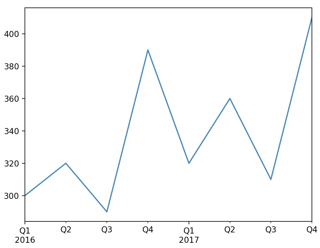
We can create a Series with a
PeriodIndex:quarterly_revenue = pd.Series([300, 320, 290, 390, 320, 360, 310, 410], index = quarters) quarterly_revenue- which outputs:
2016Q1 300 2016Q2 320 2016Q3 290 2016Q4 390 2017Q1 320 2017Q2 360 2017Q3 310 2017Q4 410 -
Plotting this data:
quarterly_revenue.plot(kind="line") plt.show()- which outputs:
-
We can convert periods to timestamps by calling
to_timestamp. By default this will give us the first day of each period, but by settinghowandfreq, we can get the last hour of each period:last_hours = quarterly_revenue.to_pd.Timestamp(how="end", freq="H") last_hours- which outputs:
2016-03-31 23:59:59.999999999 300 2016-06-30 23:59:59.999999999 320 2016-09-30 23:59:59.999999999 290 2016-12-31 23:59:59.999999999 390 2017-03-31 23:59:59.999999999 320 2017-06-30 23:59:59.999999999 360 2017-09-30 23:59:59.999999999 310 2017-12-31 23:59:59.999999999 410 Freq: Q-DEC, dtype: int64 -
And back to periods by calling
to_period:last_hours.to_period()- which outputs:
2016Q1 300 2016Q2 320 2016Q3 290 2016Q4 390 2017Q1 320 2017Q2 360 2017Q3 310 2017Q4 410 Freq: Q-DEC, dtype: int64 -
Pandas also provides many other time-related functions that we recommend you check out in the documentation. To whet your appetite, here is one way to get the last business day of each month in 2016, at 9am:
months_2016 = pd.period_range("2016", periods=12, freq="M") one_day_after_last_days = months_2016.asfreq("D") + 1 last_bdays = one_day_after_last_days.to_pd.Timestamp() - pd.tseries.offsets.BDay() last_bdays.to_period("H") + 9- which outputs:
  PeriodIndex(['2016-01-29 09:00', '2016-02-29 09:00', '2016-03-31 09:00',
               '2016-04-29 09:00', '2016-05-31 09:00', '2016-06-30 09:00',
               '2016-07-29 09:00', '2016-08-31 09:00', '2016-09-30 09:00',
               '2016-10-31 09:00', '2016-11-30 09:00', '2016-12-30 09:00'],
              dtype='period[H]', freq='H')
DataFrame objects
- A DataFrame object represents a spreadsheet, with cell values, column names and row index labels. You can define expressions to compute columns based on other columns, create pivot-tables, group rows, draw graphs, etc. You can see DataFrames as dictionaries of Series.
Creating a DataFrame
-
You can create a DataFrame by passing a dictionary of Series objects:
import pandas as pd people_dict = { "weight": pd.Series([68, 83, 112], index=["alice", "bob", "charles"]), "birthyear": pd.Series([1984, 1985, 1992], index=["bob", "alice", "charles"], name="year"), "children": pd.Series([0, 3], index=["charles", "bob"]), "hobby": pd.Series(["Biking", "Dancing"], index=["alice", "bob"]), } people = pd.DataFrame(people_dict) people- which outputs:
weight birthyear children hobby alice 68 1985 NaN Biking bob 83 1984 3.0 Dancing charles 112 1992 0.0 NaN - A few things to note:
- The Series were automatically aligned based on their index,
- Missing values are represented as
NaN, - Series names are ignored (the name
"year"was dropped), - DataFrames are displayed nicely in Jupyter notebooks, woohoo!
-
You can access columns pretty much as you would expect. They are returned as Series objects:
people["birthyear"]- which outputs:
alice 1985 bob 1984 charles 1992 Name: birthyear, dtype: int64 -
You can also get multiple columns at once:
people[["birthyear", "hobby"]]- which outputs:
birthyear hobby alice 1985 Biking bob 1984 Dancing charles 1992 NaN -
If you pass a list of columns and/or index row labels to the DataFrame constructor, it will guarantee that these columns and/or rows will exist, in that order, and no other column/row will exist. For example:
d2 = pd.DataFrame( people_dict, columns=["birthyear", "weight", "height"], index=["bob", "alice", "eugene"] ) d2- which outputs:
birthyear weight height bob 1984.0 83.0 NaN alice 1985.0 68.0 NaN eugene NaN NaN NaN -
Another convenient way to create a DataFrame is to pass all the values to the constructor as an
ndarray, or a list of lists, and specify the column names and row index labels separately:import numpy as np values = [ [1985, np.nan, "Biking", 68], [1984, 3, "Dancing", 83], [1992, 0, np.nan, 112] ] d3 = pd.DataFrame( values, columns=["birthyear", "children", "hobby", "weight"], index=["alice", "bob", "charles"] ) d3- which outputs:
birthyear children hobby weight alice 1985 NaN Biking 68 bob 1984 3.0 Dancing 83 charles 1992 0.0 NaN 112 -
To specify missing values, you can either use
np.nanor NumPy’s masked arrays:masked_array = np.ma.asarray(values, dtype=np.object) masked_array[(0, 2), (1, 2)] = np.ma.masked d3 = pd.DataFrame( masked_array, columns=["birthyear", "children", "hobby", "weight"], index=["alice", "bob", "charles"] ) d3- which outputs:
birthyear children hobby weight alice 1985 NaN Biking 68 bob 1984 3 Dancing 83 charles 1992 0 NaN 112 -
Instead of an
ndarray, you can also pass a DataFrame object:d4 = pd.DataFrame( d3, columns=["hobby", "children"], index=["alice", "bob"] ) d4- which outputs:
hobby children alice Biking NaN bob Dancing 3 -
It is also possible to create a DataFrame with a dictionary (or list) of dictionaries (or list):
people = pd.DataFrame({ "birthyear": {"alice":1985, "bob": 1984, "charles": 1992}, "hobby": {"alice":"Biking", "bob": "Dancing"}, "weight": {"alice":68, "bob": 83, "charles": 112}, "children": {"bob": 3, "charles": 0} }) people- which outputs:
           birthyear    hobby  weight  children
  alice         1985   Biking      68       NaN
  bob           1984  Dancing      83       3.0
  charles       1992      NaN     112       0.0
Multi-indexing
-
If all columns are tuples of the same size, then they are understood as a multi-index. The same goes for row index labels. For example:
import pandas as pd import numpy as np d5 = pd.DataFrame( { ("public", "birthyear"): {("Paris","alice"):1985, ("Paris","bob"): 1984, ("London","charles"): 1992}, ("public", "hobby"): {("Paris","alice"):"Biking", ("Paris","bob"): "Dancing"}, ("private", "weight"): {("Paris","alice"):68, ("Paris","bob"): 83, ("London","charles"): 112}, ("private", "children"): {("Paris", "alice"):np.nan, ("Paris","bob"): 3, ("London","charles"): 0} } ) d5- which outputs:
public private birthyear hobby weight children Paris alice 1985 Biking 68 NaN bob 1984 Dancing 83 3.0 London charles 1992 NaN 112 0.0 -
You can now get a DataFrame containing all the
"public"columns by simply doing:d5["public"]- which outputs:
birthyear hobby Paris alice 1985 Biking bob 1984 Dancing London charles 1992 NaN -
You can also now get a DataFrame containing all the
"hobby"columns within the"public"columns by simply doing:d5["public", "hobby"] # Same result as d5["public"]["hobby"]- which outputs:
  Paris   alice       Biking
          bob        Dancing
  London  charles        NaN
  Name: (public, hobby), dtype: object
Dropping a level
-
Let’s look at
d5again:import pandas as pd import numpy as np d5 = pd.DataFrame({('public', 'birthyear'): {('Paris', 'alice'): 1985, ('Paris', 'bob'): 1984, ('London', 'charles'): 1992}, ('public', 'hobby'): {('Paris', 'alice'): 'Biking', ('Paris', 'bob'): 'Dancing', ('London', 'charles'): np.nan}, ('private', 'weight'): {('Paris', 'alice'): 68, ('Paris', 'bob'): 83, ('London', 'charles'): 112}, ('private', 'children'): {('Paris', 'alice'): np.nan, ('Paris', 'bob'): 3.0, ('London', 'charles'): 0.0}})- which outputs:
public private birthyear hobby weight children Paris alice 1985 Biking 68 NaN bob 1984 Dancing 83 3.0 London charles 1992 NaN 112 0.0 -
There are two levels of columns, and two levels of indices. We can drop a column level by calling
droplevel()(the same goes for indices):d5.columns = d5.columns.droplevel(level = 0) d5- which outputs:
                  birthyear    hobby  weight  children
  Paris  alice         1985   Biking      68       NaN
         bob           1984  Dancing      83       3.0
  London charles       1992      NaN     112       0.0
Transposing
-
You can swap columns and indices using the
Tattribute, similar to NumPy:import pandas as pd d5 = pd.DataFrame({'birthyear': {('Paris', 'alice'): 1985, ('Paris', 'bob'): 1984, ('London', 'charles'): 1992}, 'hobby': {('Paris', 'alice'): 'Biking', ('Paris', 'bob'): 'Dancing', ('London', 'charles'): nan}, 'weight': {('Paris', 'alice'): 68, ('Paris', 'bob'): 83, ('London', 'charles'): 112}, 'children': {('Paris', 'alice'): nan, ('Paris', 'bob'): 3.0, ('London', 'charles'): 0.0}}) d6 = d5.T d6- which outputs:
              Paris           London
              alice      bob charles
  birthyear    1985     1984    1992
  hobby      Biking  Dancing     NaN
  weight         68       83     112
  children      NaN        3       0
Stacking and unstacking levels
-
Calling the
stack()method will push the lowest column level after the lowest index:import pandas as pd d6 = pd.DataFrame({('Paris', 'alice'): {'birthyear': 1985, 'hobby': 'Biking', 'weight': 68, 'children': nan}, ('Paris', 'bob'): {'birthyear': 1984, 'hobby': 'Dancing', 'weight': 83, 'children': 3.0}, ('London', 'charles'): {'birthyear': 1992, 'hobby': nan, 'weight': 112, 'children': 0.0}}) d7 = d6.stack() d7- which outputs:
London Paris birthyear alice NaN 1985 bob NaN 1984 charles 1992 NaN hobby alice NaN Biking bob NaN Dancing weight alice NaN 68 bob NaN 83 charles 112 NaN children bob NaN 3 charles 0 NaN - Note that many
NaNvalues appeared. This makes sense because many new combinations did not exist before (eg. there was nobobinLondon). -
Calling
unstack()will do the reverse, once again creating manyNaNvalues.d8 = d7.unstack() d8- which outputs:
London Paris alice bob charles alice bob charles birthyear NaN NaN 1992 1985 1984 NaN hobby NaN NaN NaN Biking Dancing NaN weight NaN NaN 112 68 83 NaN children NaN NaN 0 NaN 3 NaN -
If we call
unstackagain, we end up with a Series object:d9 = d8.unstack() d9- which outputs:
London alice birthyear NaN hobby NaN weight NaN children NaN bob birthyear NaN hobby NaN weight NaN children NaN charles birthyear 1992 hobby NaN weight 112 children 0 Paris alice birthyear 1985 hobby Biking weight 68 children NaN bob birthyear 1984 hobby Dancing weight 83 children 3 charles birthyear NaN hobby NaN weight NaN children NaN dtype: object -
The
stack()andunstack()methods let you select thelevelto stack/unstack. You can even stack/unstack multiple levels at once:d10 = d9.unstack(level = (0,1)) d10- which outputs:
            London                Paris
             alice  bob charles   alice      bob charles
  birthyear    NaN  NaN    1992    1985     1984     NaN
  hobby        NaN  NaN     NaN  Biking  Dancing     NaN
  weight       NaN  NaN     112      68       83     NaN
  children     NaN  NaN       0     NaN        3     NaN
Most pandas methods return modified copies
- As you may have noticed, the
stack()andunstack()methods do not modify the object they apply to. Instead, they work on a copy and return that copy. This is true of most methods in pandas.
Accessing rows
-
Let’s go back to the
peopleDataFrame:import pandas as pd people_dict = { "birthyear": pd.Series([1984, 1985, 1992], index=["bob", "alice", "charles"], name="year"), "hobby": pd.Series(["Biking", "Dancing"], index=["alice", "bob"]), "weight": pd.Series([68, 83, 112], index=["alice", "bob", "charles"]), "children": pd.Series([0, 3], index=["charles", "bob"]), } people = pd.DataFrame(people_dict) people- which outputs:
birthyear hobby weight children alice 1985 Biking 68 NaN bob 1984 Dancing 83 3.0 charles 1992 NaN 112 0.0 -
The
locattribute lets you access rows instead of columns. The result is a Series object in which the DataFrame’s column names are mapped to row index labels:people.loc["charles"]- which outputs:
birthyear 1992 hobby NaN weight 112 children 0 Name: charles, dtype: object -
You can also access rows by integer location using the
ilocattribute to get the same effect:people.iloc[2]- which outputs:
birthyear 1992 hobby NaN weight 112 children 0 Name: charles, dtype: object -
You can also get a slice of rows, and this returns a DataFrame object:
people.iloc[1:3]- which outputs:
birthyear hobby weight children bob 1984 Dancing 83 3.0 charles 1992 NaN 112 0.0 - You can also directly subscript the DataFrame using
[]to select rows (and also slice them). Thus,df[1:3]is the same asdf.iloc[1:3], which selects rows 1 and 2. Note, however, if you slice rows withloc, instead ofiloc, you’ll get rows 1, 2 and 3 assuming you have a RangeIndex. See details here.)- However, note that
[]cannot be used to slice columns as indf.loc[:, 'A':'C']. More importantly, if your selection involves both rows and columns, then assignment becomes problematic (more details in the below section).
- However, note that
-
Finally, you can pass a boolean “mask” array to get the matching rows:
people[np.array([True, False, True])]- which outputs:
birthyear hobby weight children alice 1985 Biking 68 NaN charles 1992 NaN 112 0.0 -
This is most useful when combined with boolean expressions:
people[people["birthyear"] < 1990]- which outputs:
         birthyear    hobby  weight  children
  alice       1985   Biking      68       NaN
  bob         1984  Dancing      83       3.0
Accessing columns
- There are three methods of selecting a column in a Pandas DataFrame.
- Using
loc[:, <col>]:df_new = df.loc[:, 'col1'] - Subscripting using
[]:df_new = df['col1'] - Accessing the column as a member variable of the DataFrame using
.:df_new = df.col1
- Using
- As such, selecting a single column (
df['A']is the same asdf.loc[:, 'A']-> selects columnA). Similarly, selecting a list of columns (df[['A', 'B', 'C']]is the same asdf.loc[:, ['A', 'B', 'C']]-> selects columnsA, B and C). - However, note that
[]does not work in the following situations:- You can select a single row with
df.loc[row_label] - You can select a list of rows with
df.loc[[row_label1, row_label2]]
- You can select a single row with
-
More importantly, as mentioned in the earlier section, if your selection involves both rows and columns, then assignment becomes problematic.
df[1:3]['A'] = 5 -
This selects rows 1 and 2 then selects column ‘A’ of the returning object and assigns value 5 to it. The problem is, the returning object might be a copy so this may not change the actual DataFrame. This raises
SettingWithCopyWarning. The correct way of making this assignment is:df.loc[1:3, 'A'] = 5 - With
.loc(), you are guaranteed to modify the original DataFrame. It also allows you to slice columns (df.loc[:, 'C':'F']), select a single row (df.loc[5]), and select a list of rows (df.loc[[1, 2, 5]]).
Adding and removing columns
-
Again, let’s go back to the
peopleDataFrame:import pandas as pd people_dict = { "birthyear": pd.Series([1984, 1985, 1992], index=["bob", "alice", "charles"], name="year"), "hobby": pd.Series(["Biking", "Dancing"], index=["alice", "bob"]), "weight": pd.Series([68, 83, 112], index=["alice", "bob", "charles"]), "children": pd.Series([0, 3], index=["charles", "bob"]), } people = pd.DataFrame(people_dict) people- which outputs:
birthyear hobby weight children alice 1985 Biking 68 NaN bob 1984 Dancing 83 3.0 charles 1992 NaN 112 0.0 -
You can generally treat DataFrame objects like dictionaries of Series, so adding new columns can be accomplished using:
people["age"] = 2018 - people["birthyear"] # adds a new column "age" people["over 30"] = people["age"] > 30 # adds another column "over 30" birthyears = people.pop("birthyear") del people["children"] people- which outputs:
hobby weight age over 30 alice Biking 68 33 True bob Dancing 83 34 True charles NaN 112 26 False -
We can print
birthyearsusing:birthyears- which outputs:
alice 1985 bob 1984 charles 1992 Name: birthyear, dtype: int64 -
When you add a new column, it must have the same number of rows. Missing rows are filled with NaN, and extra rows are ignored:
people["pets"] = pd.Series({"bob": 0, "charles": 5, "eugene": 1}) # alice is missing, eugene is ignored people- which outputs:
hobby weight age over 30 pets alice Biking 68 33 True NaN bob Dancing 83 34 True 0.0 charles NaN 112 26 False 5.0 -
When adding a new column, it is added at the end (on the right) by default. You can also insert a column anywhere else using the
insert()method:people.insert(1, "height", [172, 181, 185]) people- which outputs:
             hobby  height  weight  age  over 30  pets
  alice     Biking     172      68   33     True   NaN
  bob      Dancing     181      83   34     True   0.0
  charles      NaN     185     112   26    False   5.0
Assigning new columns
-
Again, let’s go back to the
peopleDataFrame:import pandas as pd people_dict = { "hobby": pd.Series(["Biking", "Dancing"], index=["alice", "bob"]), "height": pd.Series([172, 181, 185], index=["alice", "bob", "charles"]), "weight": pd.Series([68, 83, 112], index=["alice", "bob", "charles"]), "age": pd.Series([33, 34, 26], index=["alice", "bob", "charles"]), "over 30": pd.Series([True, True, False], index=["alice", "bob", "charles"]), "pets": pd.Series({"bob": 0.0, "charles": 5.0}), } people = pd.DataFrame(people_dict) people- which outputs:
hobby height weight age over 30 pets alice Biking 172 68 33 True NaN bob Dancing 181 83 34 True 0.0 charles NaN 185 112 26 False 5.0 -
You can also create new columns by calling the
assign()method. Note that this returns a new DataFrame object, the original is not modified:people.assign( body_mass_index = people["weight"] / (people["height"] / 100) ** 2, has_pets = people["pets"] > 0 )- which outputs:
weight height hobby age over 30 pets body_mass_index has_pets alice 68 172 Biking 33 True NaN 22.985398 False bob 83 181 Dancing 34 True 0.0 25.335002 False charles 112 185 NaN 26 False 5.0 32.724617 True -
Note that you cannot access columns created within the same assignment:
try: people.assign( body_mass_index = people["weight"] / (people["height"] / 100) ** 2, overweight = people["body_mass_index"] > 25 ) except KeyError as e: print("Key error:", e)- which outputs:
Key error: 'body_mass_index' -
The solution is to split this assignment in two consecutive assignments:
d6 = people.assign(body_mass_index = people["weight"] / (people["height"] / 100) ** 2) d6.assign(overweight = d6["body_mass_index"] > 25)- which outputs:
hobby height weight age over 30 pets body_mass_index overweight alice Biking 172 68 33 True NaN 22.985398 False bob Dancing 181 83 34 True 0.0 25.335002 True charles NaN 185 112 26 False 5.0 32.724617 True -
Having to create a temporary variable
d6is not very convenient. You may want to just chain the assigment calls, but it does not work because thepeopleobject is not actually modified by the first assignment:try: (people .assign(body_mass_index = people["weight"] / (people["height"] / 100) ** 2) .assign(overweight = people["body_mass_index"] > 25) ) except KeyError as e: print("Key error:", e)- which outputs:
Key error: 'body_mass_index' -
But fear not, there is a simple solution. You can pass a function to the
assign()method (typically alambdafunction), and this function will be called with the DataFrame as a parameter:(people .assign(body_mass_index = lambda df: df["weight"] / (df["height"] / 100) ** 2) .assign(overweight = lambda df: df["body_mass_index"] > 25) )- which outputs:
hobby height weight age over 30 pets body_mass_index overweight alice Biking 172 68 33 True NaN 22.985398 False bob Dancing 181 83 34 True 0.0 25.335002 True charles NaN 185 112 26 False 5.0 32.724617 True- Problem solved!
Evaluating an expression
-
A great feature supported by pandas is expression evaluation. This relies on the
numexprlibrary which must be installed.import pandas as pd people = pd.DataFrame({'hobby': {'alice': 'Biking', 'bob': 'Dancing', 'charles': nan}, 'height': {'alice': 172, 'bob': 181, 'charles': 185}, 'weight': {'alice': 68, 'bob': 83, 'charles': 112}, 'age': {'alice': 33, 'bob': 34, 'charles': 26}, 'over 30': {'alice': True, 'bob': True, 'charles': False}, 'pets': {'alice': nan, 'bob': 0.0, 'charles': 5.0}}) people.eval("weight / (height/100) ** 2 > 25")- which outputs:
alice False bob True charles True dtype: bool -
Assignment expressions are also supported. Let’s set
inplace=Trueto directly modify the DataFrame rather than getting a modified copy:people.eval("body_mass_index = weight / (height/100) ** 2", inplace=True) people- which outputs:
hobby height weight age over 30 pets body_mass_index alice Biking 172 68 33 True NaN 22.985398 bob Dancing 181 83 34 True 0.0 25.335002 charles NaN 185 112 26 False 5.0 32.724617 -
You can use a local or global variable in an expression by prefixing it with
'@':overweight_threshold = 30 people.eval("overweight = body_mass_index > @overweight_threshold", inplace=True) people- which outputs:
             hobby  height  weight  age  over 30  pets  body_mass_index  overweight
  alice     Biking     172      68   33     True   NaN        22.985398       False
  bob      Dancing     181      83   34     True   0.0        25.335002       False
  charles      NaN     185     112   26    False   5.0        32.724617        True
Querying a DataFrame
-
The
query()method lets you filter a DataFrame based on a query expression:import pandas as pd people = pd.DataFrame({'hobby': {'alice': 'Biking', 'bob': 'Dancing', 'charles': nan}, 'height': {'alice': 172, 'bob': 181, 'charles': 185}, 'weight': {'alice': 68, 'bob': 83, 'charles': 112}, 'age': {'alice': 33, 'bob': 34, 'charles': 26}, 'over 30': {'alice': True, 'bob': True, 'charles': False}, 'pets': {'alice': nan, 'bob': 0.0, 'charles': 5.0}, 'body_mass_index': {'alice': 22.985397512168742, 'bob': 25.33500198406642, 'charles': 32.72461650840029}, 'overweight': {'alice': False, 'bob': False, 'charles': True}}) people.query("age > 30 and pets == 0")- which outputs:
         hobby  height  weight  age  over 30  pets  body_mass_index  overweight
  bob  Dancing     181      83   34     True   0.0        25.335002       False
Sorting a DataFrame
-
You can sort a DataFrame by calling its
sort_indexmethod. By default, it sorts the rows by their index label in ascending order, but let’s reverse the order:import pandas as pd people = pd.DataFrame({'hobby': {'alice': 'Biking', 'bob': 'Dancing', 'charles': nan}, 'height': {'alice': 172, 'bob': 181, 'charles': 185}, 'weight': {'alice': 68, 'bob': 83, 'charles': 112}, 'age': {'alice': 33, 'bob': 34, 'charles': 26}, 'over 30': {'alice': True, 'bob': True, 'charles': False}, 'pets': {'alice': nan, 'bob': 0.0, 'charles': 5.0}, 'body_mass_index': {'alice': 22.985397512168742, 'bob': 25.33500198406642, 'charles': 32.72461650840029}, 'overweight': {'alice': False, 'bob': False, 'charles': True}}) people.sort_index(ascending=False)- which outputs:
hobby height weight age over 30 pets body_mass_index overweight charles NaN 185 112 26 False 5.0 32.724617 True bob Dancing 181 83 34 True 0.0 25.335002 False alice Biking 172 68 33 True NaN 22.985398 False -
Note that
sort_indexreturned a sorted copy of the DataFrame. To modifypeopledirectly, we can set theinplaceargument toTrue. Also, we can sort the columns instead of the rows by settingaxis=1:people.sort_index(axis=1, inplace=True) people- which outputs:
age body_mass_index height hobby over 30 overweight pets weight alice 33 22.985398 172 Biking True False NaN 68 bob 34 25.335002 181 Dancing True False 0.0 83 charles 26 32.724617 185 NaN False True 5.0 112 -
To sort the DataFrame by the values instead of the labels, we can use
sort_valuesand specify the column to sort by:people.sort_values(by="age", inplace=True) people- which outputs:
           age  body_mass_index  height    hobby  over 30  overweight  pets  weight
  charles   26        32.724617     185      NaN    False        True   5.0     112
  alice     33        22.985398     172   Biking     True       False   NaN      68
  bob       34        25.335002     181  Dancing     True       False   0.0      83
Plotting a DataFrame
- Just like for Series, pandas makes it easy to draw nice graphs based on a DataFrame.
-
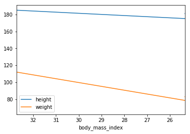
For example, it is trivial to create a line plot from a DataFrame’s data by calling its
plotmethod:import matplotlib.pyplot as plt import pandas as pd import numpy as np people = pd.DataFrame({'age': {'charles': 26, 'alice': 33, 'bob': 34}, 'body_mass_index': {'charles': 32.72461650840029, 'alice': 22.985397512168742, 'bob': 25.33500198406642}, 'height': {'charles': 185, 'alice': 172, 'bob': 181}, 'hobby': {'charles': np.nan, 'alice': 'Biking', 'bob': 'Dancing'}, 'over 30': {'charles': False, 'alice': True, 'bob': True}, 'overweight': {'charles': True, 'alice': False, 'bob': False}, 'pets': {'charles': 5.0, 'alice': np.nan, 'bob': 0.0}, 'weight': {'charles': 112, 'alice': 68, 'bob': 83}}) people.plot(kind = "line", x = "body_mass_index", y = ["height", "weight"]) plt.show()- which outputs:
-
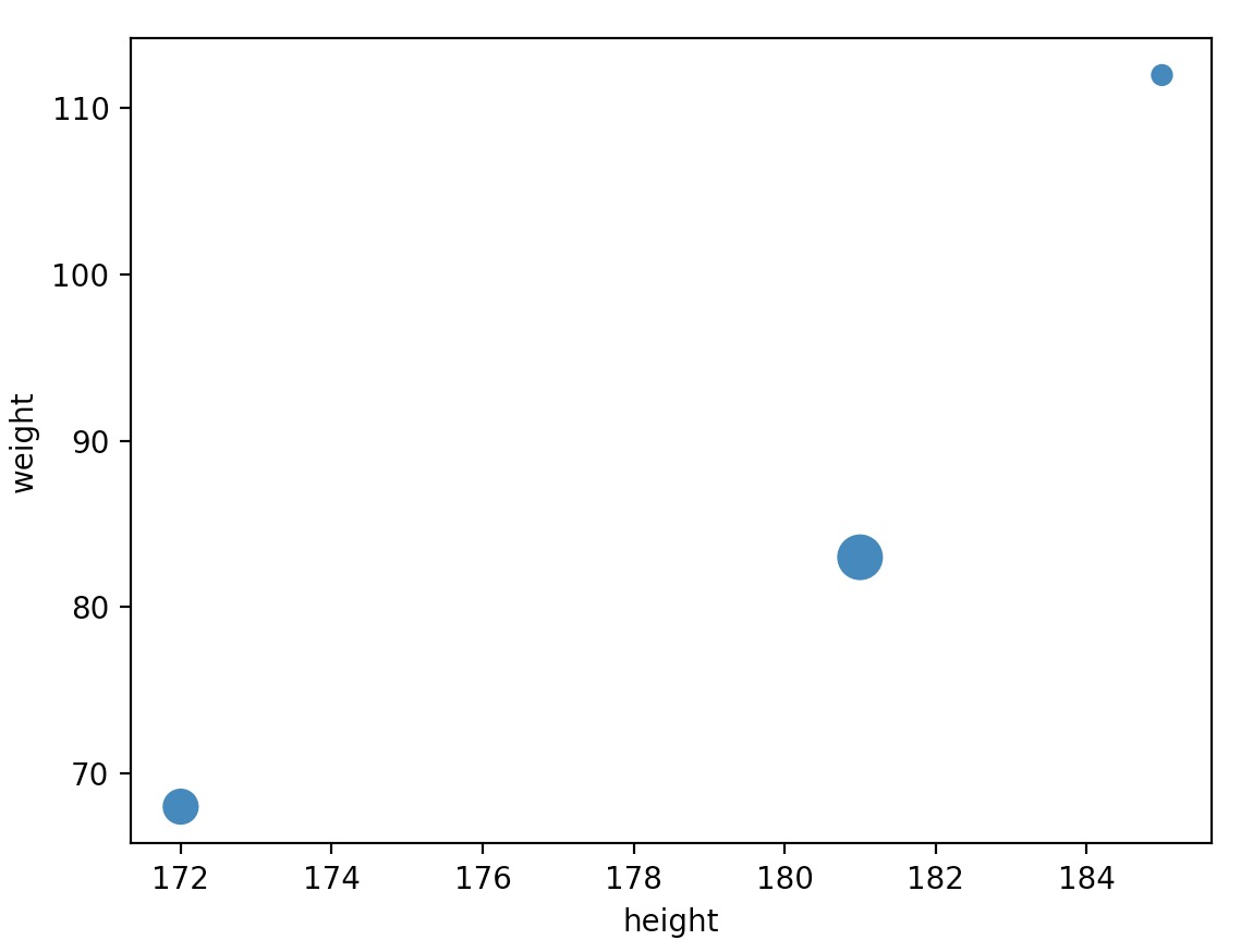
You can pass extra arguments supported by matplotlib’s functions. For example, we can create scatterplot and pass it a list of sizes using the
sargument of matplotlib’sscatter()function:people.plot(kind = "scatter", x = "height", y = "weight", s=[40, 120, 200]) plt.show()- which outputs:
- Again, there are way too many options to list here: the best option is to scroll through the Visualization page in pandas’ documentation, find the plot you are interested in and look at the example code.
Operations on DataFrames
-
Although DataFrames do not try to mimick NumPy arrays, there are a few similarities. Let’s create a DataFrame to demonstrate this:
import pandas as pd grades_array = np.array([[8, 8, 9], [10, 9, 9], [4, 8, 2], [9, 10, 10]]) grades = pd.DataFrame(grades_array, columns=["sep", "oct", "nov"], index=["alice","bob","charles","darwin"]) grades- which outputs:
sep oct nov alice 8 8 9 bob 10 9 9 charles 4 8 2 darwin 9 10 10 -
You can apply NumPy mathematical functions on a DataFrame: the function is applied to all values:
np.sqrt(grades)- which outputs:
sep oct nov alice 2.828427 2.828427 3.000000 bob 3.162278 3.000000 3.000000 charles 2.000000 2.828427 1.414214 darwin 3.000000 3.162278 3.162278 -
Similarly, adding a single value to a DataFrame will add that value to all elements in the DataFrame. This is called broadcasting:
grades + 1- which outputs:
sep oct nov alice 9 9 10 bob 11 10 10 charles 5 9 3 darwin 10 11 11 -
Of course, the same is true for all other binary operations, including arithmetic (
*,/,**…) and conditional (>,==…) operations:grades >= 5- which outputs:
sep oct nov alice True True True bob True True True charles False True False darwin True True True -
Aggregation operations, such as computing the
max, thesumor themeanof a DataFrame, apply to each column, and you get back a Series object:grades.mean()- which outputs:
sep 7.75 oct 8.75 nov 7.50 dtype: float64 -
The
allmethod is also an aggregation operation: it checks whether all values areTrueor not. Let’s see during which months all students got a grade greater than5:(grades > 5).all()- which outputs:
sep False oct True nov False dtype: bool -
Most of these functions take an optional
axisparameter which lets you specify along which axis of the DataFrame you want the operation executed. The default isaxis=0, meaning that the operation is executed vertically (on each column). You can setaxis=1to execute the operation horizontally (on each row). For example, let’s find out which students had all grades greater than5:(grades > 5).all(axis = 1)- which outputs:
alice True bob True charles False darwin True dtype: bool -
The
anymethod returnsTrueif any value is true. Let’s see who got at least one grade 10:(grades == 10).any(axis = 1)- which outputs:
alice False bob True charles False darwin True dtype: bool -
If you add a Series object to a DataFrame (or execute any other binary operation), pandas attempts to broadcast the operation to all rows in the DataFrame. This only works if the Series has the same size as the DataFrames rows. For example, let’s subtract the
meanof the DataFrame (a Series object) from the DataFrame:grades - grades.mean() # equivalent to: grades - [7.75, 8.75, 7.50]- which outputs:
sep oct nov alice 0.25 -0.75 1.5 bob 2.25 0.25 1.5 charles -3.75 -0.75 -5.5 darwin 1.25 1.25 2.5 -
We subtracted
7.75from all September grades,8.75from October grades and7.50from November grades. It is equivalent to substracting this DataFrame:pd.DataFrame([[7.75, 8.75, 7.50]]*4, index=grades.index, columns=grades.columns)- which outputs:
sep oct nov alice 7.75 8.75 7.5 bob 7.75 8.75 7.5 charles 7.75 8.75 7.5 darwin 7.75 8.75 7.5 -
If you want to subtract the global mean from every grade, here is one way to do it:
grades - grades.values.mean() # subtracts the global mean (8.00) from all grades- which outputs:
           sep  oct  nov
  alice    0.0  0.0  1.0
  bob      2.0  1.0  1.0
  charles -4.0  0.0 -6.0
  darwin   1.0  2.0  2.0
Automatic alignment
-
Similar to Series, when operating on multiple DataFrames, pandas automatically aligns them by row index label, but also by column names. Let’s start with our previous grades DataFrame to demonstrate this:
import pandas as pd grades_array = np.array([[8, 8, 9], [10, 9, 9], [4, 8, 2], [9, 10, 10]]) grades = pd.DataFrame(grades_array, columns=["sep", "oct", "nov"], index=["alice", "bob", "charles", "darwin"]) grades- which outputs:
sep oct nov alice 8 8 9 bob 10 9 9 charles 4 8 2 darwin 9 10 10 -
Now, let’s create a new DataFrame that holds the bonus points for each person from October to December:
import numpy as np bonus_array = np.array([[0, np.nan, 2],[np.nan, 1, 0],[0, 1, 0], [3, 3, 0]]) bonus_points = pd.DataFrame(bonus_array, columns=["oct", "nov", "dec"], index=["bob", "colin", "darwin", "charles"]) bonus_points- which outputs:
oct nov dec bob 0.0 NaN 2.0 colin NaN 1.0 0.0 darwin 0.0 1.0 0.0 charles 3.0 3.0 0.0 -
Now, let’s combine both DataFrames:
grades + bonus_points- which outputs:
dec nov oct sep alice NaN NaN NaN NaN bob NaN NaN 9.0 NaN charles NaN 5.0 11.0 NaN colin NaN NaN NaN NaN darwin NaN 11.0 10.0 NaN -
Looks like the addition worked in some cases but way too many elements are now empty. That’s because when aligning the DataFrames, some columns and rows were only present on one side, and thus they were considered missing on the other side (
NaN). Then addingNaNto a number results inNaN, hence the result.
Handling missing data
- Dealing with missing data is a frequent task when working with real life data. Pandas offers a few tools to handle missing data.
-
Let’s try to fix the problem seen in the above section on automatic alignment. Let’s start with our previous grades DataFrame to demonstrate this:
import pandas as pd grades = pd.DataFrame({'sep': {'alice': 8, 'bob': 10, 'charles': 4, 'darwin': 9}, 'oct': {'alice': 8, 'bob': 9, 'charles': 8, 'darwin': 10}, 'nov': {'alice': 9, 'bob': 9, 'charles': 2, 'darwin': 10}}) grades- which outputs:
sep oct nov alice 8 8 9 bob 10 9 9 charles 4 8 2 darwin 9 10 10 -
Now, let’s create a new DataFrame that holds the bonus points for each person from October to December:
import numpy as np bonus_points = pd.DataFrame({'oct': {'bob': 0.0, 'colin': np.nan, 'darwin': 0.0, 'charles': 3.0}, 'nov': {'bob': np.nan, 'colin': 1.0, 'darwin': 1.0, 'charles': 3.0}, 'dec': {'bob': 2.0, 'colin': 0.0, 'darwin': 0.0, 'charles': 0.0}}) bonus_points- which outputs:
oct nov dec bob 0.0 NaN 2.0 colin NaN 1.0 0.0 darwin 0.0 1.0 0.0 charles 3.0 3.0 0.0 -
For example, we can decide that missing data should result in a zero, instead of
NaN. We can replace allNaNvalues by a any value using thefillna()method:(grades + bonus_points).fillna(0)- which outputs:
dec nov oct sep alice 0.0 0.0 0.0 0.0 bob 0.0 0.0 9.0 0.0 charles 0.0 5.0 11.0 0.0 colin 0.0 0.0 0.0 0.0 darwin 0.0 11.0 10.0 0.0 -
It’s a bit unfair that we’re setting grades to zero in September, though. Perhaps we should decide that missing grades are missing grades, but missing bonus points should be replaced by zeros:
fixed_bonus_points = bonus_points.fillna(0) fixed_bonus_points.insert(0, "sep", 0) fixed_bonus_points.loc["alice"] = 0 grades + fixed_bonus_points- which outputs:
dec nov oct sep alice NaN 9.0 8.0 8.0 bob NaN 9.0 9.0 10.0 charles NaN 5.0 11.0 4.0 colin NaN NaN NaN NaN darwin NaN 11.0 10.0 9.0 - That’s much better: although we made up some data, we have not been too unfair.
-
Another way to handle missing data is to interpolate. Let’s look at the
bonus_pointsDataFrame again:bonus_points- which outputs:
oct nov dec bob 0.0 NaN 2.0 colin NaN 1.0 0.0 darwin 0.0 1.0 0.0 charles 3.0 3.0 0.0 -
Now let’s call the
interpolatemethod. By default, it interpolates vertically (axis=0), so let’s tell it to interpolate horizontally (axis=1).bonus_points.interpolate(axis=1)- which outputs:
oct nov dec bob 0.0 1.0 2.0 colin NaN 1.0 0.0 darwin 0.0 1.0 0.0 charles 3.0 3.0 0.0 -
Bob had 0 bonus points in October, and 2 in December. When we interpolate for November, we get the mean: 1 bonus point. Colin had 1 bonus point in November, but we do not know how many bonus points he had in September, so we cannot interpolate, this is why there is still a missing value in October after interpolation. To fix this, we can set the September bonus points to 0 before interpolation.
better_bonus_points = bonus_points.copy() better_bonus_points.insert(0, "sep", 0) better_bonus_points.loc["alice"] = 0 better_bonus_points = better_bonus_points.interpolate(axis=1) better_bonus_points- which outputs:
sep oct nov dec bob 0.0 0.0 1.0 2.0 colin 0.0 0.5 1.0 0.0 darwin 0.0 0.0 1.0 0.0 charles 0.0 3.0 3.0 0.0 alice 0.0 0.0 0.0 0.0 -
Great, now we have reasonable bonus points everywhere. Let’s find out the final grades:
grades + better_bonus_points- which outputs:
dec nov oct sep alice NaN 9.0 8.0 8.0 bob NaN 10.0 9.0 10.0 charles NaN 5.0 11.0 4.0 colin NaN NaN NaN NaN darwin NaN 11.0 10.0 9.0 -
It is slightly annoying that the September column ends up on the right. This is because the DataFrames we are adding do not have the exact same columns (the
gradesDataFrame is missing the"dec"column), so to make things predictable, pandas orders the final columns alphabetically. To fix this, we can simply add the missing column before adding:import numpy as np grades["dec"] = np.nan final_grades = grades + better_bonus_points final_grades- which outputs:
sep oct nov dec alice 8.0 8.0 9.0 NaN bob 10.0 9.0 10.0 NaN charles 4.0 11.0 5.0 NaN colin NaN NaN NaN NaN darwin 9.0 10.0 11.0 NaN -
There’s not much we can do about December and Colin: it’s bad enough that we are making up bonus points, but we can’t reasonably make up grades (well I guess some teachers probably do). So let’s call the
dropna()method to get rid of rows that are full ofNaNs:final_grades_clean = final_grades.dropna(how="all") final_grades_clean- which outputs:
sep oct nov dec alice 8.0 8.0 9.0 NaN bob 10.0 9.0 10.0 NaN charles 4.0 11.0 5.0 NaN darwin 9.0 10.0 11.0 NaN -
Now let’s remove columns that are full of
NaNs by setting theaxisargument to1:final_grades_clean = final_grades_clean.dropna(axis=1, how="all") final_grades_clean- which outputs:
            sep   oct   nov
  alice     8.0   8.0   9.0
  bob      10.0   9.0  10.0
  charles   4.0  11.0   5.0
  darwin    9.0  10.0  11.0
Aggregating using groupby
-
Similar to the SQL language, pandas allows grouping your data into groups to run calculations over each group.
-
First, let’s add some extra data about each person so we can group them, and let’s go back to the
final_gradesDataFrame so we can see howNaNvalues are handled:import pandas as pd import numpy as np final_grades = pd.DataFrame({'sep': {'alice': 8.0, 'bob': 10.0, 'charles': 4.0, 'colin': np.nan, 'darwin': 9.0}, 'oct': {'alice': 8.0, 'bob': 9.0, 'charles': 11.0, 'colin': np.nan, 'darwin': 10.0}, 'nov': {'alice': 9.0, 'bob': 10.0, 'charles': 5.0, 'colin': np.nan, 'darwin': 11.0}, 'dec': {'alice': np.nan, 'bob': np.nan, 'charles': np.nan, 'colin': np.nan, 'darwin': np.nan}}) final_grades- which outputs:
sep oct nov dec alice 8.0 8.0 9.0 NaN bob 10.0 9.0 10.0 NaN charles 4.0 11.0 5.0 NaN colin NaN NaN NaN NaN darwin 9.0 10.0 11.0 NaN -
Adding a new column “hobby” to
final_grades:final_grades["hobby"] = ["Biking", "Dancing", np.nan, "Dancing", "Biking"] final_grades- which outputs:
sep oct nov dec hobby alice 8.0 8.0 9.0 NaN Biking bob 10.0 9.0 10.0 NaN Dancing charles 4.0 11.0 5.0 NaN NaN colin NaN NaN NaN NaN Dancing darwin 9.0 10.0 11.0 NaN Biking -
Now let’s group data in this DataFrame by hobby:
grouped_grades = final_grades.groupby("hobby") grouped_grades- which outputs:
<pandas.core.groupby.generic.DataFrameGroupBy object at [address]> -
We are ready to compute the average grade per hobby:
grouped_grades.mean()- which outputs:
sep oct nov dec hobby Biking 8.5 9.0 10.0 NaN Dancing 10.0 9.0 10.0 NaN -
That was easy! Note that the
NaNvalues have simply been skipped when computing the means.
Group DataFrame’s Rows into a List Using groupby
-
It is common to use
groupbyto get the statistics of rows in the same group such as count, mean, median, etc. If you want to group rows into a list instead, uselambda x: list(x).import pandas as pd df = pd.DataFrame( { "col1": [1, 2, 3, 4, 3], "col2": ["a", "a", "b", "b", "c"], "col3": ["d", "e", "f", "g", "h"], } ) df.groupby(["col2"]).agg({"col1": "mean", "col3": lambda x: list(x)})- which outputs:
        col1    col3
  col2
  a      1.5  [d, e]
  b      3.5  [f, g]
  c      3.0     [h]
Get the N Largest Values for Each Category in a DataFrame
-
If you want to get the
nlargest values for each category in a pandas DataFrame, use the combination ofgroupbyandnlargest.import pandas as pd df = pd.DataFrame({"type": ["a", "a", "a", "b", "b"], "value": [1, 2, 3, 1, 2]}) # Get n largest values for each type ( df.groupby("type") .apply(lambda df_: df_.nlargest(2, "value")) .reset_index(drop=True) )- which outputs:
  type    value
  0   a   3
  1   a   2
  2   b   2
  3   b   1
Assign Name to a Pandas Aggregation
-
By default, aggregating a column returns the name of that column.
import pandas as pd df = pd.DataFrame({"size": ["S", "S", "M", "L"], "price": [2, 3, 4, 5]}) df.groupby('size').agg({'price': 'mean'})- which outputs:
price size L 5.0 M 4.0 S 2.5 -
If you want to assign a new name to an aggregation, add
name = (column, agg_method)toagg.df.groupby('size').agg(mean_price=('price', 'mean'))- which outputs:
        mean_price
  size
  L            5.0
  M            4.0
  S            2.5
pd.pivot_table(): Turn Your DataFrame Into a Pivot Table
- A pivot table is useful to summarize and analyze the patterns in your data.
- Pandas supports spreadsheet-like pivot tables that allow quick data summarization. If you want to turn your DataFrame into a pivot table, use
pd.pivot_table(). -
To illustrate this, let’s start with a DataFrame:
final_grades_clean = {'sep': {'alice': 8.0, 'bob': 10.0, 'charles': 4.0, 'darwin': 9.0}, 'oct': {'alice': 8.0, 'bob': 9.0, 'charles': 11.0, 'darwin': 10.0}, 'nov': {'alice': 9.0, 'bob': 10.0, 'charles': 5.0, 'darwin': 11.0}} final_grades_clean- which outputs:
oct nov dec bob 0.0 NaN 2.0 colin NaN 1.0 0.0 darwin 0.0 1.0 0.0 charles 3.0 3.0 0.0 -
Now let’s restructure the data:
more_grades = final_grades_clean.stack().reset_index() more_grades.columns = ["name", "month", "grade"] more_grades["bonus"] = [np.nan, np.nan, np.nan, 0, np.nan, 2, 3, 3, 0, 0, 1, 0] more_grades- which outputs:
name month grade bonus 0 alice sep 8.0 NaN 1 alice oct 8.0 NaN 2 alice nov 9.0 NaN 3 bob sep 10.0 0.0 4 bob oct 9.0 NaN 5 bob nov 10.0 2.0 6 charles sep 4.0 3.0 7 charles oct 11.0 3.0 8 charles nov 5.0 0.0 9 darwin sep 9.0 0.0 10 darwin oct 10.0 1.0 11 darwin nov 11.0 0.0 -
Now we can call the
pd.pivot_table()function for this DataFrame, asking to group by thenamecolumn. By default,pivot_table()computes the mean of each numeric column:pd.pivot_table(more_grades, index="name")- which outputs:
bonus grade name alice NaN 8.333333 bob 1.000000 9.666667 charles 2.000000 6.666667 darwin 0.333333 10.000000 -
We can change the aggregation function by setting the
aggfuncargument, and we can also specify the list of columns whose values will be aggregated:pd.pivot_table(more_grades, index="name", values=["grade","bonus"], aggfunc=np.max)- which outputs:
bonus grade name alice NaN 9.0 bob 2.0 10.0 charles 3.0 11.0 darwin 1.0 11.0 -
We can also specify the
columnsto aggregate over horizontally, and request the grand totals for each row and column by settingmargins=True:pd.pivot_table(more_grades, index="name", values="grade", columns="month", margins=True)- which outputs:
month nov oct sep All name alice 9.00 8.0 8.00 8.333333 bob 10.00 9.0 10.00 9.666667 charles 5.00 11.0 4.00 6.666667 darwin 11.00 10.0 9.00 10.000000 All 8.75 9.5 7.75 8.666667 -
Finally, we can specify multiple index or column names, and pandas will create multi-level indices:
pd.pivot_table(more_grades, index=("name", "month"), margins=True)- which outputs:
bonus grade name month alice nov NaN 9.00 oct NaN 8.00 sep NaN 8.00 bob nov 2.000 10.00 oct NaN 9.00 sep 0.000 10.00 charles nov 0.000 5.00 oct 3.000 11.00 sep 3.000 4.00 darwin nov 0.000 11.00 oct 1.000 10.00 sep 0.000 9.00 All 1.125 8.75 -
As another example:
import pandas as pd df = pd.DataFrame( { "item": ["apple", "apple", "apple", "apple", "apple"], "size": ["small", "small", "large", "large", "large"], "location": ["Walmart", "Aldi", "Walmart", "Aldi", "Aldi"], "price": [3, 2, 4, 3, 2.5], } ) df- which outputs:
item size location price 0 apple small Walmart 3.0 1 apple small Aldi 2.0 2 apple large Walmart 4.0 3 apple large Aldi 3.0 4 apple large Aldi 2.5- Applying
pd.pivot_table():
pivot = pd.pivot_table( df, values="price", index=["item", "size"], columns=["location"], aggfunc="mean" ) pivot- which outputs:
location Aldi Walmart item size apple large 2.75 4.0 small 2.00 3.0
Overview functions
-
When dealing with large
DataFrames, it is useful to get a quick overview of its content. Pandas offers a few functions for this. First, let’s create a large DataFrame with a mix of numeric values, missing values and text values. Notice how Jupyter displays only the corners of the DataFrame:much_data = np.fromfunction(lambda x,y: (x+y*y)%17*11, (10000, 26)) large_df = pd.DataFrame(much_data, columns=list("ABCDEFGHIJKLMNOPQRSTUVWXYZ")) large_df[large_df % 16 == 0] = np.nan large_df.insert(3,"some_text", "Blabla") large_df- which outputs:
A B C some_text D ... V W X Y Z 0 NaN 11.0 44.0 Blabla 99.0 ... NaN 88.0 22.0 165.0 143.0 1 11.0 22.0 55.0 Blabla 110.0 ... NaN 99.0 33.0 NaN 154.0 2 22.0 33.0 66.0 Blabla 121.0 ... 11.0 110.0 44.0 NaN 165.0 3 33.0 44.0 77.0 Blabla 132.0 ... 22.0 121.0 55.0 11.0 NaN 4 44.0 55.0 88.0 Blabla 143.0 ... 33.0 132.0 66.0 22.0 NaN ... ... ... ... ... ... ... ... ... ... ... ... 9995 NaN NaN 33.0 Blabla 88.0 ... 165.0 77.0 11.0 154.0 132.0 9996 NaN 11.0 44.0 Blabla 99.0 ... NaN 88.0 22.0 165.0 143.0 9997 11.0 22.0 55.0 Blabla 110.0 ... NaN 99.0 33.0 NaN 154.0 9998 22.0 33.0 66.0 Blabla 121.0 ... 11.0 110.0 44.0 NaN 165.0 9999 33.0 44.0 77.0 Blabla 132.0 ... 22.0 121.0 55.0 11.0 NaN [10000 rows x 27 columns] -
The
head()method returns the top 5 rows:large_df.head()- which outputs:
A B C some_text D ... V W X Y Z 0 NaN 11.0 44.0 Blabla 99.0 ... NaN 88.0 22.0 165.0 143.0 1 11.0 22.0 55.0 Blabla 110.0 ... NaN 99.0 33.0 NaN 154.0 2 22.0 33.0 66.0 Blabla 121.0 ... 11.0 110.0 44.0 NaN 165.0 3 33.0 44.0 77.0 Blabla 132.0 ... 22.0 121.0 55.0 11.0 NaN 4 44.0 55.0 88.0 Blabla 143.0 ... 33.0 132.0 66.0 22.0 NaN [5 rows x 27 columns] -
Similarly, there’s also a
tail()function to view the bottom 5 rows. You can pass the number of rows you want:large_df.tail(n=2)- which outputs:
A B C some_text D ... V W X Y Z 9998 22.0 33.0 66.0 Blabla 121.0 ... 11.0 110.0 44.0 NaN 165.0 9999 33.0 44.0 77.0 Blabla 132.0 ... 22.0 121.0 55.0 11.0 NaN [2 rows x 27 columns] -
The
info()method prints out a summary of each columns contents:large_df.info()- which outputs:
<class 'pandas.core.frame.DataFrame'> RangeIndex: 10000 entries, 0 to 9999 Data columns (total 27 columns): A 8823 non-null float64 B 8824 non-null float64 C 8824 non-null float64 some_text 10000 non-null object D 8824 non-null float64 E 8822 non-null float64 F 8824 non-null float64 G 8824 non-null float64 H 8822 non-null float64 I 8823 non-null float64 J 8823 non-null float64 K 8822 non-null float64 L 8824 non-null float64 M 8824 non-null float64 N 8822 non-null float64 O 8824 non-null float64 P 8824 non-null float64 Q 8824 non-null float64 R 8823 non-null float64 S 8824 non-null float64 T 8824 non-null float64 U 8824 non-null float64 V 8822 non-null float64 W 8824 non-null float64 X 8824 non-null float64 Y 8822 non-null float64 Z 8823 non-null float64 dtypes: float64(26), object(1) memory usage: 2.1+ MB -
Finally, the
describe()method gives a nice overview of the main aggregated values over each column:count: number of non-null (not NaN) valuesmean: mean of non-null valuesstd: standard deviation of non-null valuesmin: minimum of non-null values25%,50%,75%: 25th, 50th and 75th percentile of non-null valuesmax: maximum of non-null values
large_df.describe()- which outputs:
A B ... Y Z count 8823.000000 8824.000000 ... 8822.000000 8823.000000 mean 87.977559 87.972575 ... 88.000000 88.022441 std 47.535911 47.535523 ... 47.536879 47.535911 min 11.000000 11.000000 ... 11.000000 11.000000 25% 44.000000 44.000000 ... 44.000000 44.000000 50% 88.000000 88.000000 ... 88.000000 88.000000 75% 132.000000 132.000000 ... 132.000000 132.000000 max 165.000000 165.000000 ... 165.000000 165.000000 [8 rows x 26 columns]
Saving and loading
-
Pandas can save DataFrames to various backends, including file formats such as CSV, Excel, JSON, HTML and HDF5, or to a SQL database. Let’s create a DataFrame to demonstrate this:
my_df = pd.DataFrame( [["Biking", 68.5, 1985, np.nan], ["Dancing", 83.1, 1984, 3]], columns=["hobby","weight","birthyear","children"], index=["alice", "bob"] ) my_df- which outputs:
hobby weight birthyear children alice Biking 68.5 1985 NaN bob Dancing 83.1 1984 3.0
Saving
-
Let’s save it to CSV, HTML and JSON:
my_df.to_csv("my_df.csv") my_df.to_html("my_df.html") my_df.to_json("my_df.json") -
Done! Let’s take a peek at what was saved:
for filename in ("my_df.csv", "my_df.html", "my_df.json"): print("##", filename) with open(filename, "rt") as f: print(f.read()) print()- which outputs:
## my_df.csv ,hobby,weight,birthyear,children alice,Biking,68.5,1985, bob,Dancing,83.1,1984,3.0 ## my_df.html <table border="1" class="dataframe"> <thead> <tr style="text-align: right;"> <th></th> <th>hobby</th> <th>weight</th> <th>birthyear</th> <th>children</th> </tr> </thead> <tbody> <tr> <th>alice</th> <td>Biking</td> <td>68.5</td> <td>1985</td> <td>NaN</td> </tr> <tr> <th>bob</th> <td>Dancing</td> <td>83.1</td> <td>1984</td> <td>3.0</td> </tr> </tbody> </table> ## my_df.json {"hobby":{"alice":"Biking","bob":"Dancing"},"weight":{"alice":68.5,"bob":83.1},"birthyear":{"alice":1985,"bob":1984},"children":{"alice":null,"bob":3.0}} -
Note that the index is saved as the first column (with no name) in a CSV file, as
<th>tags in HTML and as keys in JSON. -
Saving to other formats works very similarly, but some formats require extra libraries to be installed. For example, saving to Excel requires the
openpyxllibrary:try: my_df.to_excel("my_df.xlsx", sheet_name='People') except ImportError as e: print(e)- which outputs:
No module named 'openpyxl'
Loading
-
Now let’s load our CSV file back into a DataFrame:
my_df_loaded = pd.read_csv("my_df.csv", index_col=0) my_df_loaded- which outputs:
hobby weight birthyear children alice Biking 68.5 1985 NaN bob Dancing 83.1 1984 3.0 -
As you might guess, there are similar
read_json,read_html,read_excelfunctions as well. We can also read data straight from the Internet. For example, let’s load all U.S. cities from simplemaps.com:us_cities = None try: csv_url = "https://raw.githubusercontent.com/datasets/world-cities/master/data/world-cities.csv" us_cities = pd.read_csv(csv_url, index_col=0) us_cities = us_cities.head() except IOError as e: print(e) us_cities- which outputs:
country subcountry geonameid name les Escaldes Andorra Escaldes-Engordany 3040051 Andorra la Vella Andorra Andorra la Vella 3041563 Umm al Qaywayn United Arab Emirates Umm al Qaywayn 290594 Ras al-Khaimah United Arab Emirates Raʼs al Khaymah 291074 Khawr Fakkān United Arab Emirates Ash Shāriqah 291696 -
There are more options available, in particular regarding datetime format. Check out the documentation for more details.
Combining DataFrames
SQL-like joins
- One powerful feature of pandas is it’s ability to perform SQL-like joins on DataFrames. Various types of joins are supported: inner joins, left/right outer joins and full joins. To illustrate this, let’s start by creating a couple of simple DataFrames.
-
Here’s the city_loc DataFrame:
city_loc = pd.DataFrame( [ ["CA", "San Francisco", 37.781334, -122.416728], ["NY", "New York", 40.705649, -74.008344], ["FL", "Miami", 25.791100, -80.320733], ["OH", "Cleveland", 41.473508, -81.739791], ["UT", "Salt Lake City", 40.755851, -111.896657] ], columns=["state", "city", "lat", "lng"]) city_loc- which outputs:
state city lat lng 0 CA San Francisco 37.781334 -122.416728 1 NY New York 40.705649 -74.008344 2 FL Miami 25.791100 -80.320733 3 OH Cleveland 41.473508 -81.739791 4 UT Salt Lake City 40.755851 -111.896657city_pop = pd.DataFrame( [ [808976, "San Francisco", "California"], [8363710, "New York", "New-York"], [413201, "Miami", "Florida"], [2242193, "Houston", "Texas"] ], index=[3,4,5,6], columns=["population", "city", "state"]) city_pop- which outputs:
population city state 3 808976 San Francisco California 4 8363710 New York New-York 5 413201 Miami Florida 6 2242193 Houston Texas -
Now let’s join these DataFrames using the
merge()function:pd.merge(left=city_loc, right=city_pop, on="city")- which outputs:
state_x city lat lng population state_y 0 CA San Francisco 37.781334 -122.416728 808976 California 1 NY New York 40.705649 -74.008344 8363710 New-York 2 FL Miami 25.791100 -80.320733 413201 Florida -
Note that both DataFrames have a column named
state, so in the result they got renamed tostate_xandstate_y. -
Also, note that Cleveland, Salt Lake City and Houston were dropped because they don’t exist in both DataFrames. This is the equivalent of a SQL
INNER JOIN. If you want aFULL OUTER JOIN, where no city gets dropped andNaNvalues are added, you must specifyhow="outer":all_cities = pd.merge(left=city_loc, right=city_pop, on="city", how="outer") all_cities- which outputs:
state_x city lat lng population state_y 0 CA San Francisco 37.781334 -122.416728 808976.0 California 1 NY New York 40.705649 -74.008344 8363710.0 New-York 2 FL Miami 25.791100 -80.320733 413201.0 Florida 3 OH Cleveland 41.473508 -81.739791 NaN NaN 4 UT Salt Lake City 40.755851 -111.896657 NaN NaN 5 NaN Houston NaN NaN 2242193.0 Texas -
Of course
LEFT OUTER JOINis also available by settinghow="left": only the cities present in the left DataFrame end up in the result. Similarly, withhow="right"only cities in the right DataFrame appear in the result. For example:pd.merge(left=city_loc, right=city_pop, on="city", how="right")- which outputs:
state_x city lat lng population state_y 0 CA San Francisco 37.781334 -122.416728 808976 California 1 NY New York 40.705649 -74.008344 8363710 New-York 2 FL Miami 25.791100 -80.320733 413201 Florida 3 NaN Houston NaN NaN 2242193 Texas -
If the key to join on is actually in one (or both) DataFrame’s index, you must use
left_index=Trueand/orright_index=True. If the key column names differ, you must useleft_onandright_on. For example:city_pop2 = city_pop.copy() city_pop2.columns = ["population", "name", "state"] pd.merge(left=city_loc, right=city_pop2, left_on="city", right_on="name")- which outputs:
state_x city lat ... population name state_y 0 CA San Francisco 37.781334 ... 808976 San Francisco California 1 NY New York 40.705649 ... 8363710 New York New-York 2 FL Miami 25.791100 ... 413201 Miami Florida [3 rows x 7 columns]
Concatenation
-
Rather than joining DataFrames, we may just want to concatenate them. That’s what
concat()is for:result_concat = pd.concat([city_loc, city_pop]) result_concat- which outputs:
city lat lng population state 0 San Francisco 37.781334 -122.416728 NaN CA 1 New York 40.705649 -74.008344 NaN NY 2 Miami 25.791100 -80.320733 NaN FL 3 Cleveland 41.473508 -81.739791 NaN OH 4 Salt Lake City 40.755851 -111.896657 NaN UT 3 San Francisco NaN NaN 808976.0 California 4 New York NaN NaN 8363710.0 New-York 5 Miami NaN NaN 413201.0 Florida 6 Houston NaN NaN 2242193.0 Texas -
Note that this operation aligned the data horizontally (by columns) but not vertically (by rows). In this example, we end up with multiple rows having the same index (eg. 3). Pandas handles this rather gracefully:
result_concat.loc[3]- which outputs:
city lat lng population state 3 Cleveland 41.473508 -81.739791 NaN OH 3 San Francisco NaN NaN 808976.0 California -
Or you can tell pandas to just ignore the index:
pd.concat([city_loc, city_pop], ignore_index=True)- which outputs:
city lat lng population state 0 San Francisco 37.781334 -122.416728 NaN CA 1 New York 40.705649 -74.008344 NaN NY 2 Miami 25.791100 -80.320733 NaN FL 3 Cleveland 41.473508 -81.739791 NaN OH 4 Salt Lake City 40.755851 -111.896657 NaN UT 5 San Francisco NaN NaN 808976.0 California 6 New York NaN NaN 8363710.0 New-York 7 Miami NaN NaN 413201.0 Florida 8 Houston NaN NaN 2242193.0 Texas -
Notice that when a column does not exist in a DataFrame, it acts as if it was filled with
NaNvalues. If we setjoin="inner", then only columns that exist in both DataFrames are returned:pd.concat([city_loc, city_pop], join="inner")- which outputs:
state city 0 CA San Francisco 1 NY New York 2 FL Miami 3 OH Cleveland 4 UT Salt Lake City 3 California San Francisco 4 New-York New York 5 Florida Miami 6 Texas Houston -
You can concatenate DataFrames horizontally instead of vertically by setting
axis=1:pd.concat([city_loc, city_pop], axis=1)- which outputs:
state city lat ... population city state 0 CA San Francisco 37.781334 ... NaN NaN NaN 1 NY New York 40.705649 ... NaN NaN NaN 2 FL Miami 25.791100 ... NaN NaN NaN 3 OH Cleveland 41.473508 ... 808976.0 San Francisco California 4 UT Salt Lake City 40.755851 ... 8363710.0 New York New-York 5 NaN NaN NaN ... 413201.0 Miami Florida 6 NaN NaN NaN ... 2242193.0 Houston Texas [7 rows x 7 columns] -
In this case it really does not make much sense because the indices do not align well (eg. Cleveland and San Francisco end up on the same row, because they shared the index label
3). So let’s reindex the DataFrames by city name before concatenating:pd.concat([city_loc.set_index("city"), city_pop.set_index("city")], axis=1)- which outputs:
state lat lng population state Cleveland OH 41.473508 -81.739791 NaN NaN Houston NaN NaN NaN 2242193.0 Texas Miami FL 25.791100 -80.320733 413201.0 Florida New York NY 40.705649 -74.008344 8363710.0 New-York Salt Lake City UT 40.755851 -111.896657 NaN NaN San Francisco CA 37.781334 -122.416728 808976.0 California - This looks a lot like a
FULL OUTER JOIN, except that thestatecolumns were not renamed tostate_xandstate_y, and thecitycolumn is now the index. -
The
append()method is a useful shorthand for concatenating DataFrames vertically:city_loc.append(city_pop)- which outputs:
city lat lng population state 0 San Francisco 37.781334 -122.416728 NaN CA 1 New York 40.705649 -74.008344 NaN NY 2 Miami 25.791100 -80.320733 NaN FL 3 Cleveland 41.473508 -81.739791 NaN OH 4 Salt Lake City 40.755851 -111.896657 NaN UT 3 San Francisco NaN NaN 808976.0 California 4 New York NaN NaN 8363710.0 New-York 5 Miami NaN NaN 413201.0 Florida 6 Houston NaN NaN 2242193.0 Texas - As always in pandas, the
append()method does not actually modifycity_loc: it works on a copy and returns the modified copy.
Categories
-
It is quite frequent to have values that represent categories, for example
1for female and2for male, or"A"for Good,"B"for Average,"C"for Bad. These categorical values can be hard to read and cumbersome to handle, but fortunately pandas makes it easy. To illustrate this, let’s take thecity_popDataFrame we created earlier, and add a column that represents a category:city_eco = city_pop.copy() city_eco["eco_code"] = [17, 17, 34, 20] city_eco- which outputs:
population city state eco_code 3 808976 San Francisco California 17 4 8363710 New York New-York 17 5 413201 Miami Florida 34 6 2242193 Houston Texas 20 -
Right now the
eco_codecolumn is full of apparently meaningless codes. Let’s fix that. First, we will create a new categorical column based on theeco_codes:city_eco["economy"] = city_eco["eco_code"].astype('category') city_eco["economy"].cat.categories- which outputs:
Int64Index([17, 20, 34], dtype='int64') -
Now we can give each category a meaningful name:
city_eco["economy"].cat.categories = ["Finance", "Energy", "Tourism"] city_eco- which outputs:
population city state eco_code economy 3 808976 San Francisco California 17 Finance 4 8363710 New York New-York 17 Finance 5 413201 Miami Florida 34 Tourism 6 2242193 Houston Texas 20 Energy -
Note that categorical values are sorted according to their categorical order (and not their alphabetical order):
city_eco.sort_values(by="economy", ascending=False)- which outputs:
population city state eco_code economy 5 413201 Miami Florida 34 Tourism 6 2242193 Houston Texas 20 Energy 3 808976 San Francisco California 17 Finance 4 8363710 New York New-York 17 Finance
Practical example using a sample dataset
- To demonstrate the use of pandas, we’ll be using the interview reviews scraped from Glassdoor in 2019. The data is available here.
Dataset at a glance
-
Let’s check out the dataset :
import pandas as pd df = pd.read_csv("../assets/pandas/interviews.csv") print(df.shape) df.head()- which outputs:
Company Title Job Level Date Upvotes Offer Experience Difficulty Review 0 Apple Software Engineer Software Engineer Engineer Aug 7, 2019 0 No offer 0.0 Medium Application I applied through a staffing agen... 1 Apple Software Engineer Software Engineer Engineer Aug 8, 2019 0 Accepted offer 1.0 Hard Application I applied online. The process too... 2 Apple Software Engineer Software Engineer Engineer NaN 0 Declined offer 0.0 Medium Application The process took 4 weeks. I inter... 3 Apple Software Engineer Software Engineer Engineer NaN 9 Declined offer -1.0 Medium Application The process took a week. I interv... 4 Apple Software Engineer Software Engineer Engineer May 29, 2009 2 No offer 0.0 Medium Application I applied through an employee ref...
Iterating over rows
.apply()
- pandas documentation has a warning box that basically tells you not to iterate over rows because it’s slow.
- Before iterating over rows, think about what you want to do with each row, pack that into a function and use methods like
.apply()to apply the function to all rows. - For example, to scale the “Experience” column by the number of “Upvotes” each review has, one way is to iterate over rows and multiple the “Upvotes” value by the “Experience” value of that row. But you can also use
.apply()with alambdafunction. -
Run the following code snippet in a Colab/Jupyter notebook:
%timeit -n1 df.apply(lambda x: x["Experience"] * x["Upvotes"], axis=1)- which outputs:
180 ms ± 16.5 ms per loop (mean ± std. dev. of 7 runs, 1 loop each)
.iterrows() and .itertuples()
-
If you really want to iterate over rows, one naive way is to use
.iterrows(). It returns a generator that generates row by row and it’s very slow. Run the following code snippet in a Colab/Jupyter notebook:%timeit -n1 [row for index, row in df.iterrows()]- which outputs:
1.42 s ± 107 ms per loop (mean ± std. dev. of 7 runs, 1 loop each) -
Using
.iterrows():# This is what a row looks like as a pandas object for index, row in df.iterrows(): print(row) break- which outputs:
Company Apple Title Software Engineer Job Software Engineer Level Engineer Date Aug 7, 2019 Upvotes 0 Offer No offer Experience 0 Difficulty Medium Review Application I applied through a staffing agen... Name: 0, dtype: object -
.itertuples()returns rows in thenamedtupleformat. It still lets you access each row and it’s about 40x faster than.iterrows(). Run the following code snippet in a Colab/Jupyter notebook:%timeit -n1 [row for row in df.itertuples()]- which outputs:
24.2 ms ± 709 µs per loop (mean ± std. dev. of 7 runs, 1 loop each) -
Using
.iterrows():# This is what a row looks like as a namedtuple. for row in df.itertuples(): print(row) break- which outputs:
Pandas(Index=0, Company='Apple', Title='Software Engineer', Job='Software Engineer', Level='Engineer', Date='Aug 7, 2019', Upvotes=0, Offer='No offer', Experience=0.0, Difficulty='Medium', Review='Application I applied through a staffing agency. I interviewed at Apple (Sunnyvale, CA) in March 2019. Interview The interviewer asked me about my background. Asked few questions from the resume. Asked about my proficiency on data structures. Asked me how do you sort hashmap keys based on values. Interview Questions Write a program that uses two threads to print the numbers from 1 to n.')
Ordering slicing operations
- Because pandas is column-major, if you want to do multiple slicing operations, always do the column-based slicing operations first.
- For example, if you want to get the review from the first row of the data, there are two slicing operations:
- get row (row-based operation)
- get review (column-based operation)
- Get row -> get review is 25x slower than get review -> get row.
-
Note: You can also just use
df.loc[0, "Review"]to calculate the memory address to retrieve the item. Its performance is comparable to get review then get row.%timeit -n1000 df["Review"][0] %timeit -n1000 df.iloc[0]["Review"] %timeit -n1000 df.loc[0, "Review"]- which outputs:
5.55 µs ± 1.05 µs per loop (mean ± std. dev. of 7 runs, 1000 loops each) 136 µs ± 2.57 µs per loop (mean ± std. dev. of 7 runs, 1000 loops each) 6.23 µs ± 264 ns per loop (mean ± std. dev. of 7 runs, 1000 loops each)
SettingWithCopyWarning
-
Sometimes, when you try to assign values to a subset of data in a DataFrame, you get
SettingWithCopyWarning. Don’t ignore the warning because it means sometimes, the assignment works (example 1), but sometimes, it doesn’t (example 2). -
Example 1: Changing the review of the first row:
df["Review"][0] = "I like Orange better." # Even though with the warning, the assignment works. The review is updated. df.head(1)- which outputs:
/Users/chip/miniconda3/envs/py3/lib/python3.6/site-packages/ipykernel_launcher.py:2: SettingWithCopyWarning: A value is trying to be set on a copy of a slice from a DataFrame See the caveats in the documentation: https://pandas.pydata.org/pandas-docs/stable/user_guide/indexing.html#returning-a-view-versus-a-copy Company Title Job Level Date Upvotes Offer Experience Difficulty Review 0 Apple Software Engineer Software Engineer Engineer Aug 7, 2019 0 No offer 0.0 Medium I like Orange better. -
Example 2: Changing the company name Apple to Orange:
df[df["Company"] == "Apple"]["Company"] = "Orange" # With the warning, the assignment doesn't work. The company name is still Apple. df.head(1)- which outputs:
/Users/chip/miniconda3/envs/py3/lib/python3.6/site-packages/ipykernel_launcher.py:2: SettingWithCopyWarning: A value is trying to be set on a copy of a slice from a DataFrame. Try using .loc[row_indexer,col_indexer] = value instead See the caveats in the documentation: https://pandas.pydata.org/pandas-docs/stable/user_guide/indexing.html#returning-a-view-versus-a-copy Company Title Job Level Date Upvotes Offer Experience Difficulty Review 0 Apple Software Engineer Software Engineer Engineer Aug 7, 2019 0 No offer 0.0 Medium I like Orange better.
View vs. Copy
- To understand this weird behavior, we need to understand two concepts in pandas:
Viewvs.Copy. Viewis the actual DataFrame you want to work with.-
Copyis a copy of that actual DataFrame, which will be thrown away as soon as the operation is done. -
So if you try to do an assignment on a
Copy, the assignment won’t work. -
SettingWithCopyWarningdoesn’t mean you’re making changes to aCopy. It means that the thing you’re making changes to might be aCopyor aView, and pandas can’t tell you. -
The ambiguity happens because of
__getitem__operation.__getitem__sometimes returns aCopy, sometimes aView, and pandas makes no guarantee.# df["Review"][0] = "I like Orange better." # can be understood as # `df.__getitem__("Review").__setitem__(0, "I like Orange better.")`# df[df["Company"] == "Apple"]["Company"] = "Orange" # can be understood as # df.__getitem__(where df["Company"] == "Apple").__setitem__("Company", "Orange")
Solutions
Combine all chained operations into one single operation
- To avoid
__getitem__ambiguity, you can combine all your operations into one single operation..loc[]is usually great for that. -
Changing the review of the first row:
df.loc[0, "Review"] = "Orange is love. Orange is life." df.head()- which outputs:
Company Title Job Level Date Upvotes Offer Experience Difficulty Review 0 Apple Software Engineer Software Engineer Engineer Aug 7, 2019 0 No offer 0.0 Medium Orange is love. Orange is life. 1 Apple Software Engineer Software Engineer Engineer Aug 8, 2019 0 Accepted offer 1.0 Hard Application I applied online. The process too... 2 Apple Software Engineer Software Engineer Engineer NaN 0 Declined offer 0.0 Medium Application The process took 4 weeks. I inter... 3 Apple Software Engineer Software Engineer Engineer NaN 9 Declined offer -1.0 Medium Application The process took a week. I interv... 4 Apple Software Engineer Software Engineer Engineer May 29, 2009 2 No offer 0.0 Medium Application I applied through an employee ref... -
Changing the company name
AppletoOrange:df.loc[df["Company"] == "Apple", "Company"] = "Orange" df.head()- which outputs:
Company Title Job Level Date Upvotes Offer Experience Difficulty Review 0 Orange Software Engineer Software Engineer Engineer Aug 7, 2019 0 No offer 0.0 Medium Orange is love. Orange is life. 1 Orange Software Engineer Software Engineer Engineer Aug 8, 2019 0 Accepted offer 1.0 Hard Application I applied online. The process too... 2 Orange Software Engineer Software Engineer Engineer NaN 0 Declined offer 0.0 Medium Application The process took 4 weeks. I inter... 3 Orange Software Engineer Software Engineer Engineer NaN 9 Declined offer -1.0 Medium Application The process took a week. I interv... 4 Orange Software Engineer Software Engineer Engineer May 29, 2009 2 No offer 0.0 Medium Application I applied through an employee ref...
Raise an error
-
SettingWithCopyWarningshould ideally be an Exception instead of a warning. You can change this warning into an exception with pandas’ magicset_option().pd.set_option("mode.chained_assignment", "raise") # Running this will show you an Exception # df["Review"][0] = "I like Orange better."
Indexing and slicing
.iloc[]: selecting rows based on integer indices
.iloc[]lets you select rows by integer indices.-
Accessing the third row of a DataFrame:
df.iloc[3]- which outputs:
Company Orange Title Software Engineer Job Software Engineer Level Engineer Date NaN Upvotes 9 Offer Declined offer Experience -1 Difficulty Medium Review Application The process took a week. I interv... Name: 3, dtype: object - Slicing with
.iloc[]is similar to slicing in Python. If you want a refresher on how slicing in Python works, see our Python Tutorial. -
Selecting the last 6 rows:
df.iloc[-6:]- which outputs:
Company Title Job Level Date Upvotes Offer Experience Difficulty Review 17648 Tencent Software Engineer Software Engineer Engineer Nov 4, 2012 0 No offer NaN NaN Application I applied online. The process too... 17649 Tencent Software Engineer Software Engineer Engineer May 25, 2012 0 Declined offer 0.0 Medium Application I applied online. The process too... 17650 Tencent Software Engineer Software Engineer Engineer Mar 15, 2014 0 No offer NaN NaN Application I applied through college or univ... 17651 Tencent Software Engineer Software Engineer Engineer Sep 22, 2015 0 Accepted offer 1.0 Medium Application I applied through college or univ... 17652 Tencent Software Engineer Software Engineer Engineer Jul 4, 2017 0 Declined offer 1.0 Medium Application I applied through college or univ... 17653 Tencent Software Engineer Software Engineer Engineer Sep 30, 2016 0 Declined offer 0.0 Easy Application I applied online. The process too... -
Selecting 1 from every 2 rows in the last 6 rows:
df.iloc[-6::2]- which outputs:
Company Title Job Level Date Upvotes Offer Experience Difficulty Review 17648 Tencent Software Engineer Software Engineer Engineer Nov 4, 2012 0 No offer NaN NaN Application I applied online. The process too... 17650 Tencent Software Engineer Software Engineer Engineer Mar 15, 2014 0 No offer NaN NaN Application I applied through college or univ... 17652 Tencent Software Engineer Software Engineer Engineer Jul 4, 2017 0 Declined offer 1.0 Medium Application I applied through college or univ...
.loc[]: selecting rows by labels or boolean masks
.loc[]lets you select rows based on one of the two things:- boolean masks
- labels
Selecting rows by boolean masks
- If you want to select all the rows where candidates declined offer, you can do it with two steps:
- Create a boolean mask on whether the “Offer” column equals to “Declined offer”
- Use that mask to select rows
df.loc[df["Offer"] == "Declined offer"] # This is equivalent to: # mask = df["Offer"] == "Declined offer" # df.loc[mask] # or simply: # df.loc[df["Offer"] == "Declined offer"]- which outputs:
Company Title Job Level Date Upvotes Offer Experience Difficulty Review 2 Orange Software Engineer Software Engineer Engineer NaN 0 Declined offer 0.0 Medium Application The process took 4 weeks. I inter... 3 Orange Software Engineer Software Engineer Engineer NaN 9 Declined offer -1.0 Medium Application The process took a week. I interv... 7 Orange Software Engineer Software Engineer Engineer Jul 26, 2019 1 Declined offer -1.0 Medium Application The process took 4+ weeks. I inte... 17 Orange Software Engineer Software Engineer Engineer Feb 27, 2010 7 Declined offer -1.0 Medium Application The process took 1 day. I intervi... 65 Orange Software Engineer Software Engineer Engineer May 6, 2012 1 Declined offer 1.0 Easy Application The process took 2 days. I interv... ... ... ... ... ... ... ... ... ... ... ... 17643 Tencent Software Engineer Software Engineer Engineer Apr 9, 2016 0 Declined offer 1.0 Medium Application I applied online. I interviewed a... 17646 Tencent Software Engineer Software Engineer Engineer May 28, 2010 0 Declined offer 0.0 Easy Application I applied through an employee ref... 17649 Tencent Software Engineer Software Engineer Engineer May 25, 2012 0 Declined offer 0.0 Medium Application I applied online. The process too... 17652 Tencent Software Engineer Software Engineer Engineer Jul 4, 2017 0 Declined offer 1.0 Medium Application I applied through college or univ... 17653 Tencent Software Engineer Software Engineer Engineer Sep 30, 2016 0 Declined offer 0.0 Easy Application I applied online. The process too... [1135 rows × 10 columns]
Selecting rows by labels
Creating labels
- Currently, our DataFrame has no labels yet. To create labels, use
.set_index().- Labels can be integers or strings
- A DataFrame can have multiple labels
# Adding label "Hardware" if the company name is "Orange", "Dell", "IDM", or "Siemens". # "Orange" because we changed "Apple" to "Orange" above. # Adding label "Software" otherwise. def company_type(x): hardware_companies = set(["Orange", "Dell", "IBM", "Siemens"]) return "Hardware" if x["Company"] in hardware_companies else "Software" df["Type"] = df.apply(lambda x: company_type(x), axis=1) # Setting "Type" to be labels. We call "" df = df.set_index("Type") df # Label columns aren't considered part of the DataFrame's content. # After adding labels to your DataFrame, it still has 10 columns, same as before.- which outputs:
Company Title Job Level Date Upvotes Offer Experience Difficulty Review 0 Orange Software Engineer Software Engineer Engineer Aug 7, 2019 0 No offer 0.0 Medium Orange is love. Orange is life. 1 Orange Software Engineer Software Engineer Engineer Aug 8, 2019 0 Accepted offer 1.0 Hard Application I applied online. The process too... 2 Orange Software Engineer Software Engineer Engineer NaN 0 Declined offer 0.0 Medium Application The process took 4 weeks. I inter... 3 Orange Software Engineer Software Engineer Engineer NaN 9 Declined offer -1.0 Medium Application The process took a week. I interv... 4 Orange Software Engineer Software Engineer Engineer May 29, 2009 2 No offer 0.0 Medium Application I applied through an employee ref... ... ... ... ... ... ... ... ... ... ... ... 17649 Tencent Software Engineer Software Engineer Engineer May 25, 2012 0 Declined offer 0.0 Medium Application I applied online. The process too... 17650 Tencent Software Engineer Software Engineer Engineer Mar 15, 2014 0 No offer NaN NaN Application I applied through college or univ... 17651 Tencent Software Engineer Software Engineer Engineer Sep 22, 2015 0 Accepted offer 1.0 Medium Application I applied through college or univ... 17652 Tencent Software Engineer Software Engineer Engineer Jul 4, 2017 0 Declined offer 1.0 Medium Application I applied through college or univ... 17653 Tencent Software Engineer Software Engineer Engineer Sep 30, 2016 0 Declined offer 0.0 Easy Application I applied online. The process too... [17654 rows x 10 columns] - Warning: labels in DataFrame are stored as normal columns when you write the DataFrame to file using
.to_csv(), and will need to be explicitly set after loading files, so if you send your CSV file to other people without explaining, they’ll have no way of knowing which columns are labels. This might cause reproducibility issues. See Stack Overflow answer.
Selecting rows by labels
-
Selecting rows with label “Hardware”:
df.loc["Hardware"]- which outputs:
Company Title Job Level Date Upvotes Offer Experience Difficulty Review Type Hardware Orange Software Engineer Software Engineer Engineer Aug 7, 2019 0 No offer 0.0 Medium Orange is love. Orange is life. Hardware Orange Software Engineer Software Engineer Engineer Aug 8, 2019 0 Accepted offer 1.0 Hard Application I applied online. The process too... Hardware Orange Software Engineer Software Engineer Engineer NaN 0 Declined offer 0.0 Medium Application The process took 4 weeks. I inter... Hardware Orange Software Engineer Software Engineer Engineer NaN 9 Declined offer -1.0 Medium Application The process took a week. I interv... Hardware Orange Software Engineer Software Engineer Engineer May 29, 2009 2 No offer 0.0 Medium Application I applied through an employee ref... ... ... ... ... ... ... ... ... ... ... ... Hardware IBM Senior Software Engineer Software Engineer Senior Sep 20, 2015 0 No offer -1.0 Easy Application I applied through a recruiter. Th... Hardware IBM Senior Software Engineer Software Engineer Senior Sep 14, 2015 0 Accepted offer -1.0 Medium Application I applied in-person. The process ... Hardware IBM Senior Software Engineer Software Engineer Senior Aug 6, 2015 0 Accepted offer 1.0 Hard Application I applied through a recruiter. Th... Hardware IBM Senior Software Engineer Software Engineer Senior Dec 13, 2015 0 Accepted offer 1.0 Medium Application I applied online. The process too... Hardware IBM Senior Software Engineer Software Engineer Senior Feb 15, 2016 11 Accepted offer 1.0 Easy Application I applied online. The process too... [1676 rows × 10 columns] -
To drop a label, you need to use
reset_indexwithdrop=True:df.reset_index(drop=True, inplace=True) df- which outputs:
Company Title Job Level Date Upvotes Offer Experience Difficulty Review 0 Orange Software Engineer Software Engineer Engineer Aug 7, 2019 0 No offer 0.0 Medium Orange is love. Orange is life. 1 Orange Software Engineer Software Engineer Engineer Aug 8, 2019 0 Accepted offer 1.0 Hard Application I applied online. The process too... 2 Orange Software Engineer Software Engineer Engineer NaN 0 Declined offer 0.0 Medium Application The process took 4 weeks. I inter... 3 Orange Software Engineer Software Engineer Engineer NaN 9 Declined offer -1.0 Medium Application The process took a week. I interv... 4 Orange Software Engineer Software Engineer Engineer May 29, 2009 2 No offer 0.0 Medium Application I applied through an employee ref... ... ... ... ... ... ... ... ... ... ... ... 17649 Tencent Software Engineer Software Engineer Engineer May 25, 2012 0 Declined offer 0.0 Medium Application I applied online. The process too... 17650 Tencent Software Engineer Software Engineer Engineer Mar 15, 2014 0 No offer NaN NaN Application I applied through college or univ... 17651 Tencent Software Engineer Software Engineer Engineer Sep 22, 2015 0 Accepted offer 1.0 Medium Application I applied through college or univ... 17652 Tencent Software Engineer Software Engineer Engineer Jul 4, 2017 0 Declined offer 1.0 Medium Application I applied through college or univ... 17653 Tencent Software Engineer Software Engineer Engineer Sep 30, 2016 0 Declined offer 0.0 Easy Application I applied online. The process too... [17654 rows × 10 columns]
Slicing Series
-
Slicing pandas Series is similar to slicing in Python:
series = df.Company # The first 1000 companies, picking every 100th companies series[:1000:100]- which outputs:
0 Orange 100 Orange 200 Orange 300 Orange 400 Intel 500 Intel 600 Intel 700 Intel 800 Uber 900 Uber Name: Company, dtype: object
Accessors
string accessor
-
.strallows you to apply built-in string functions to all strings in a column (aka a pandas Series). These built-in functions come in handy when you want to do some basic string processing. For instance, if you want to lowercase all the reviews in theReviewscolumn:df["Review"].str.lower()- which outputs:
0 orange is love. orange is life. 1 application i applied online. the process too... 2 application the process took 4 weeks. i inter... 3 application the process took a week. i interv... 4 application i applied through an employee ref... ... 17649 application i applied online. the process too... 17650 application i applied through college or univ... 17651 application i applied through college or univ... 17652 application i applied through college or univ... 17653 application i applied online. the process too... Name: Review, Length: 17654, dtype: object -
Or if you want to get the length of all the reviews:
df.Review.str.len()- which outputs:
0 31 1 670 2 350 3 807 4 663 ... 17649 470 17650 394 17651 524 17652 391 17653 784 Name: Review, Length: 17654, dtype: int64 .strcan be very powerful if you use it with Regex. Imagine you want to get a sense of how long the interview process takes for each review. You notice that each review mentions how long it takes such as “the process took 4 weeks”. So you use these heuristics:- A process is short if it takes days.
- A process is average is if it takes weeks.
-
A process is long if it takes at least 4 weeks.
df.loc[df["Review"].str.contains("days"), "Process"] = "Short" df.loc[df["Review"].str.contains("week"), "Process"] = "Average" df.loc[df["Review"].str.contains("month|[4-9]+[^ ]* weeks|[1-9]\d{1,}[^ ]* weeks"), "Process"] = "Long" df[~df.Process.isna()][["Review", "Process"]]- which outputs:
Review Process 1 Application I applied online. The process too... Long 2 Application The process took 4 weeks. I inter... Long 3 Application The process took a week. I interv... Average 5 Application I applied through college or univ... Long 6 Application The process took 2 days. I interv... Short ... ... ... 17645 Application I applied online. The process too... Average 17647 Application I applied through college or univ... Average 17648 Application I applied online. The process too... Short 17649 Application I applied online. The process too... Average 17653 Application I applied online. The process too... Average [12045 rows × 2 columns] -
We want to sanity check if
Processcorresponds toReview, butReviewis cut off in the display above. To show longer columns, you can setdisplay.max_colwidthto100. Note: set_option has several great options you should check out.pd.set_option('display.max_colwidth', 100) df[~df.Process.isna()][["Review", "Process"]]- which outputs:
Review Process 1 Application I applied online. The process took 2+ months. I interviewed at Apple (San Jose, CA)... Long 2 Application The process took 4 weeks. I interviewed at Apple (San Antonio, TX) in February 2016... Long 3 Application The process took a week. I interviewed at Apple (Cupertino, CA) in December 2008. ... Average 5 Application I applied through college or university. The process took 6 weeks. I interviewed at... Long 6 Application The process took 2 days. I interviewed at Apple (Cupertino, CA) in March 2009. Int... Short ... ... ... 17645 Application I applied online. The process took a week. I interviewed at Tencent (Palo Alto, CA)... Average 17647 Application I applied through college or university. The process took 4+ weeks. I interviewed a... Average 17648 Application I applied online. The process took 2 days. I interviewed at Tencent. Interview I ... Short 17649 Application I applied online. The process took a week. I interviewed at Tencent (Beijing, Beiji... Average 17653 Application I applied online. The process took 3+ weeks. I interviewed at Tencent (Beijing, Bei... Average [12045 rows × 2 columns] -
To see the built-in functions available for
.str, use this:pd.Series.str.__dict__.keys()- which outputs:
dict_keys(['__module__', '__annotations__', '__doc__', '__init__', '_validate', '__getitem__', '__iter__', '_wrap_result', '_get_series_list', 'cat', 'split', 'rsplit', 'partition', 'rpartition', 'get', 'join', 'contains', 'match', 'fullmatch', 'replace', 'repeat', 'pad', 'center', 'ljust', 'rjust', 'zfill', 'slice', 'slice_replace', 'decode', 'encode', 'strip', 'lstrip', 'rstrip', 'wrap', 'get_dummies', 'translate', 'count', 'startswith', 'endswith', 'findall', 'extract', 'extractall', 'find', 'rfind', 'normalize', 'index', 'rindex', 'len', '_doc_args', 'lower', 'upper', 'title', 'capitalize', 'swapcase', 'casefold', 'isalnum', 'isalpha', 'isdigit', 'isspace', 'islower', 'isupper', 'istitle', 'isnumeric', 'isdecimal', '_make_accessor'])
Other accessors
- A Series object has three other accessors:
.dt: handles date formats..cat: handles categorical data..sparse: handles sparse matrices.
pd.Series._accessors- which outputs:
{'cat', 'dt', 'sparse', 'str'}
Data exploration
- When analyzing data, you might want to take a look at the data. pandas has some great built-in functions for that.
.head(), .tail(), .describe(), .info()
-
You’re probably familiar with
.head()and.tail()methods for showing the first/last rows of DataFrame. By default, five rows are shown, but you can specify the exact number.df.tail(8)- which outputs:
Company Title Job Level Date Upvotes Offer Experience Difficulty Review Process 17646 Tencent Software Engineer Software Engineer Engineer May 28, 2010 0 Declined offer 0.0 Easy Application I applied through an employee referral. The process took 1 day. I interviewed at Te... NaN 17647 Tencent Software Engineer Software Engineer Engineer Apr 11, 2019 0 Accepted offer 1.0 Medium Application I applied through college or university. The process took 4+ weeks. I interviewed a... Average 17648 Tencent Software Engineer Software Engineer Engineer Nov 4, 2012 0 No offer NaN NaN Application I applied online. The process took 2 days. I interviewed at Tencent. Interview I ... Short 17649 Tencent Software Engineer Software Engineer Engineer May 25, 2012 0 Declined offer 0.0 Medium Application I applied online. The process took a week. I interviewed at Tencent (Beijing, Beiji... Average 17650 Tencent Software Engineer Software Engineer Engineer Mar 15, 2014 0 No offer NaN NaN Application I applied through college or university. I interviewed at Tencent. Interview Prof... NaN 17651 Tencent Software Engineer Software Engineer Engineer Sep 22, 2015 0 Accepted offer 1.0 Medium Application I applied through college or university. The process took 1 day. I interviewed at T... NaN 17652 Tencent Software Engineer Software Engineer Engineer Jul 4, 2017 0 Declined offer 1.0 Medium Application I applied through college or university. I interviewed at Tencent (London, England ... NaN 17653 Tencent Software Engineer Software Engineer Engineer Sep 30, 2016 0 Declined offer 0.0 Easy Application I applied online. The process took 3+ weeks. I interviewed at Tencent (Beijing, Bei... Average -
You can generate statistics about numeric columns using
.describe().df.describe()- which outputs:
Upvotes Experience count 17654.000000 16365.000000 mean 2.298459 0.431714 std 28.252562 0.759964 min 0.000000 -1.000000 25% 0.000000 0.000000 50% 0.000000 1.000000 75% 1.000000 1.000000 max 1916.000000 1.000000 -
However, note that
.describe()ignores all non-numeric columns. It doesn’t take into account NaN values. So, the number shown incountabove is the number of non-NaN entries. -
To show non-null count and types of all columns, use
.info(). Note that pandas treats theStringtype as an object.df.info()- which outputs:
<class 'pandas.core.frame.DataFrame'> RangeIndex: 17654 entries, 0 to 17653 Data columns (total 11 columns): # Column Non-Null Count Dtype --- ------ -------------- ----- 0 Company 17654 non-null object 1 Title 17654 non-null object 2 Job 17654 non-null object 3 Level 17654 non-null object 4 Date 17652 non-null object 5 Upvotes 17654 non-null int64 6 Offer 17654 non-null object 7 Experience 16365 non-null float64 8 Difficulty 16376 non-null object 9 Review 17654 non-null object 10 Process 12045 non-null object dtypes: float64(1), int64(1), object(9) memory usage: 1.5+ MB -
You can also see how much space your DataFrame is taking up using :
import sys df.apply(sys.getsizeof)- which outputs:
Company 1126274 Title 1358305 Job 1345085 Level 1144784 Date 1212964 Upvotes 141384 Offer 1184190 Experience 141384 Difficulty 1058008 Review 20503467 Process 1274180 dtype: int64
Count unique values
-
You can get the number of unique values in a row (excluding NaN) with
nunique(). For instance, to get the number of unique companies in our data:df.Company.nunique()- which outputs:
28 -
You can also see how many reviews are for each company, sorted in descending order:
df.Company.value_counts()- which outputs:
Amazon 3469 Google 3445 Facebook 1817 Microsoft 1790 IBM 873 Cisco 787 Oracle 701 Uber 445 Yelp 404 Orange 363 Intel 338 Salesforce 313 SAP 275 Twitter 258 Dell 258 Airbnb 233 NVIDIA 229 Adobe 211 Intuit 203 PayPal 193 Siemens 182 Square 177 Samsung 159 eBay 148 Symantec 147 Snap 113 Netflix 109 Tencent 14 Name: Company, dtype: int64
Plotting
- If you want to see the break down of process lengths for different companies, you can use
.plot()with.groupby(). -
Note: Plotting in pandas is both mind-boggling and mind-blowing. If you’re not familiar, you might want to check out some tutorials, e.g. this simple tutorial or this saiyan-level pandas plotting with seaborn.
# Group the DataFrame by "Company" and "Process", count the number of elements, # then unstack by "Process", then plot a bar chart df.groupby(["Company", "Process"]).size().unstack(level=1).plot(kind="bar", figsize=(15, 8))- which outputs:
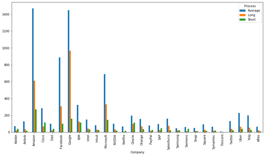
Common pitfalls
- pandas is great for most day-to-day data analysis. There is an active community that is working on regular updates to the library. However, some of the design decisions can seen a bit questionable.
- Some of the common pandas pitfalls:
NaNs as floats
- NaNs are stored as floats in pandas, so when an operation fails because of NaNs, it doesn’t say that there’s a NaN but because that operation isn’t defined for floats.
Changes aren’t in-place by default
-
Most pandas operations aren’t in-place by default, so if you make changes to your DataFrame, you need to assign the changes back to your DataFrame. You can make changes in-place by setting argument
inplace=True.# "Process" column is still in df df.drop(columns=["Process"]) df.columns- which outputs:
Index(['Company', 'Title', 'Job', 'Level', 'Date', 'Upvotes', 'Offer', 'Experience', 'Difficulty', 'Review', 'Process'], dtype='object') -
To make changes to df, set
inplace=True:df.drop(columns=["Process"], inplace=True) df.columns # This is equivalent to # df = df.drop(columns=["Process"])- which outputs:
Index(['Company', 'Title', 'Job', 'Level', 'Date', 'Upvotes', 'Offer', 'Experience', 'Difficulty', 'Review'], dtype='object')
Reproducibility issues
-
Especially with dumping and loading DataFrame to/from files. There are two main causes:
- Problem with labels (see the section about labels above).
- Weird rounding issues for floats.
GPU incompatibility
- pandas can’t take advantage of GPUs, so if your computations are on on GPUs and your feature engineering is on CPUs, it can become a time bottleneck to move data from CPUs to GPUs. If you want something like pandas but works on GPUs, check out dask and modin.
Selected Methods
Creating a DataFrame
- This section covers some pandas methods to create a new DataFrame.
Fix Unnamed:0 When Reading a CSV in pandas
-
Sometimes, when reading a CSV in pandas using
pd.read_csv(), you will get anUnnamed:0column.import pandas as pd df = pd.read_csv('data2.csv') print(df)- which outputs:
Unnamed: 0 a b 0 0 1 4 1 1 2 5 2 2 3 6 -
To fix this, add
index_col=0topandas.read_csv().df = pd.read_csv('data2.csv', index_col=0) print(df)- which outputs:
a b 0 1 4 1 2 5 2 3 6
Read HTML Tables Using Pandas
-
If you want to quickly extract a table on a website and turn it into a Pandas DataFrame, use
pd.read_html(). In the code below, we’ve extracted the table from a Wikipedia page in one line of code.import pandas as pd df = pd.read_html('https://en.wikipedia.org/wiki/Poverty') df[1]- which outputs:
Region $1 per day $1.25 per day[94] $1.90 per day[95] Region 1990 2002 2004 1981 2008 1981 1990 2000 2010 2015 2018 0 East Asia and Pacific 15.4% 12.3% 9.1% 77.2% 14.3% 80.2% 60.9% 34.8% 10.8% 2.1% 1.2% 1 Europe and Central Asia 3.6% 1.3% 1.0% 1.9% 0.5% — — 7.3% 2.4% 1.5% 1.1% 2 Latin America and the Caribbean 9.6% 9.1% 8.6% 11.9% 6.5% 13.7% 15.5% 12.7% 6% 3.7% 3.7% 3 Middle East and North Africa 2.1% 1.7% 1.5% 9.6% 2.7% — 6.5% 3.5% 2% 4.3% 7% 4 South Asia 35.0% 33.4% 30.8% 61.1% 36% 58% 49.1% — 26% — — 5 Sub-Saharan Africa 46.1% 42.6% 41.1% 51.5% 47.5% — 54.9% 58.4% 46.6% 42.3% 40.4% 6 World — — — 52.2% 22.4% 42.7% 36.2% 27.8% 16% 10.1% —- P.S.: If you run into a
Scraping: SSL: CERTIFICATE_VERIFY_FAILED errorerror when callingpd.read_html(), try running the “Install Certificates.command” file in your Python installation (located atMacintosh HD > Applications > Python<<version>)
pd.read_clipboard(): Copy CSV directly into a DataFrame
- The
pd.read_clipboard()function lets you assign data on the clipboard and passes itread_csv()(which in turn, outputs a DataFrame). - As seen in the following example, you can simply copy a table from Wikipedia and get a dataframe ready for analysis! It also works with data copied from spreadsheets and other sources.
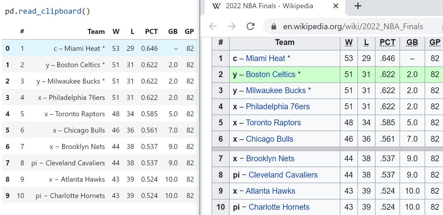
DataFrame.copy(): Make a Copy of a DataFrame
-
Have you ever tried to make a copy of a DataFrame using
=? You will not get a copy but a reference to the original DataFrame. Thus, changing the new DataFrame will also change the original DataFrame.import pandas as pd df = pd.DataFrame({'col1': [1, 2, 3], 'col2': [4, 5, 6]}) df- which outputs:
df2 = df df2['col1'] = [7, 8, 9] df -
A better way to make a copy is to use
df.copy(). Now, changing the copy will not affect the original DataFrame.df = pd.DataFrame({'col1': [1, 2, 3], 'col2': [4, 5, 6]}) # Create a copy of the original DataFrame df3 = df.copy() # Change the value of the copy df3['col1'] = [7, 8, 9] # Check if the original DataFrame has been changed df- which outputs:
col1 col2 0 1 4 1 2 5 2 3 6
DataFrame.Series.str.split: Split a String into Multiple Rows
- Sometimes, you might have a column whose values are strings representing different items such as
"1, 2".
import pandas as pd
df = pd.DataFrame({"a": ["1,2", "4,5"], "b": [11, 13]})
df
# a b
# 0 1,2 11
# 1 4,5 13
- To turn each string into a list, use
Series.str.split():
# Split by comma
df.a = df.a.str.split(",")
df
# a b
# 0 [1, 2] 11
# 1 [4, 5] 13
- Now you can split elements in the list into multiple rows using explode.
df.explode('a')
# a b
# 0 1 11
# 0 2 11
# 1 4 13
# 1 5 13
Transforming/Modifying a DataFrame
- This section covers some pandas methods to transform a DataFrame into another form, for e.g., using methods such as aggregation and groupby.
Series.map(): Change Values of a Pandas Series Using a Dictionary
- If you want to change values of a pandas Series using a dictionary, use
Series.map().
import pandas as pd
s = pd.Series(["a", "b", "c"])
s.map({"a": 1, "b": 2, "c": 3})
# 0 1
# 1 2
# 2 3
# dtype: int64
DataFrame.to_frame(): Convert Series to DataFrame
-
Convert a Series object to a DataFrame object:
import pandas as pd s = pd.Series(["a", "b", "c"], name="vals") s.to_frame() # vals # 0 a # 1 b # 2 c
DataFrame.values: Return a NumPy representation of the DataFrame
-
Only the values in the DataFrame will be returned, the axes labels will be removed.
-
A DataFrame where all columns are the same type (e.g.,
int64) results in an array of the same type:
df = pd.DataFrame({'age': [ 3, 29],
'height': [94, 170],
'weight': [31, 115]})
df
# age height weight
# 0 3 94 31
# 1 29 170 115
df.dtypes
# age int64
# height int64
# weight int64
# dtype: object
df.values
# array([[ 3, 94, 31],
# [ 29, 170, 115]])
- A DataFrame with mixed type columns (e.g.,
str/object,int64,float32) results in anndarrayof the broadest type that accommodates these mixed types (e.g.,object).
df2 = pd.DataFrame([('parrot', 24.0, 'second'),
('lion', 80.5, 1),
('monkey', np.nan, None)],
columns=('name', 'max_speed', 'rank'))
df2.dtypes
# name object
# max_speed float64
# rank object
# dtype: object
df2.values
# array([['parrot', 24.0, 'second'],
# ['lion', 80.5, 1],
# ['monkey', nan, None]], dtype=object)
DataFrame.apply(): Apply a Function to a Column of a DataFrame
DataFrame.apply()applies a function to a column of a DataFrame.
import pandas as pd
df = pd.DataFrame({"col1": [1, 2], "col2": [3, 4]})
df
# col1 col2
# 0 1 3
# 1 2 4
df["col1"] = df["col1"].apply(lambda row: row * 2)
df
# col1 col2
# 0 2 3
# 1 4 4
DataFrame.assign(): Assign Values to Multiple New Columns
DataFrame.assign()assigns new columns to a DataFrame. Returns a new object with all original columns in addition to new ones. Existing columns that are re-assigned will be overwritten.- Returns a new object with all original columns in addition to new ones. Existing columns that are re-assigned will be overwritten.
- From the official Pandas documentation:
df = pd.DataFrame({'temp_c': [17.0, 25.0]},
index=['Portland', 'Berkeley'])
df
temp_c
Portland 17.0
Berkeley 25.0
- Using
df.assignto add a newtemp_fcolumn:
df.assign(temp_f=lambda x: x.temp_c * 9 / 5 + 32)
temp_c temp_f
Portland 17.0 62.6
Berkeley 25.0 77.0
- Alternatively, the same behavior can be achieved by directly referencing an existing Series or sequence:
df.assign(temp_f=df['temp_c'] * 9 / 5 + 32)
temp_c temp_f
Portland 17.0 62.6
Berkeley 25.0 77.0
- You can create multiple columns within the same assign where one of the columns depends on another one defined within the same assign:
df.assign(temp_f=lambda x: x['temp_c'] * 9 / 5 + 32,
temp_k=lambda x: (x['temp_f'] + 459.67) * 5 / 9)
temp_c temp_f temp_k
Portland 17.0 62.6 290.15
Berkeley 25.0 77.0 298.15
Chaining multiple assigns
-
To assign values to multiple new columns, instead of assigning them separately, you can do everything in one line of code with
df.assign. -
In the code below,
col3was first created. In turn,col3was used to createcol4.
import pandas as pd
df = pd.DataFrame({"col1": [1, 2], "col2": [3, 4]})
df = df.assign(col3=lambda x: x.col1 * 100 + x.col2).assign(
col4=lambda x: x.col2 * x.col3
)
df
# col1 col2 col3 col4
# 0 1 3 103 309
# 1 2 4 204 816
DataFrame.groupby(): Group DataFrame using a mapper or by a Series of columns
- A groupby operation involves some combination of splitting the object, applying a function, and combining the results. This can be used to group large amounts of data and compute operations on these groups.
df = pd.DataFrame({'Animal': ['Falcon', 'Falcon',
'Parrot', 'Parrot'],
'Max Speed': [380., 370., 24., 26.]})
df
# Animal Max Speed
# 0 Falcon 380.0
# 1 Falcon 370.0
# 2 Parrot 24.0
# 3 Parrot 26.0
df.groupby(['Animal']).mean()
# Max Speed
# Animal
# Falcon 375.0
# Parrot 25.0
- Hierarchical Indexes:
- We can groupby different levels of a hierarchical index using the level parameter:
arrays = [['Falcon', 'Falcon', 'Parrot', 'Parrot'], ['Captive', 'Wild', 'Captive', 'Wild']] index = pd.MultiIndex.from_arrays(arrays, names=('Animal', 'Type')) df = pd.DataFrame({'Max Speed': [390., 350., 30., 20.]}, index=index) df # Max Speed # Animal Type # Falcon Captive 390.0 # Wild 350.0 # Parrot Captive 30.0 # Wild 20.0 df.groupby(level=0).mean() # Max Speed # Animal # Falcon 370.0 # Parrot 25.0 df.groupby(level="Type").mean() # Max Speed # Type # Captive 210.0 # Wild 185.0- We can also choose to include NA in group keys or not by setting dropna parameter, the default setting is True.
l = [[1, 2, 3], [1, None, 4], [2, 1, 3], [1, 2, 2]] df = pd.DataFrame(l, columns=["a", "b", "c"]) df.groupby(by=["b"]).sum() # a c # b # 1.0 2 3 # 2.0 2 5 df.groupby(by=["b"], dropna=False).sum() # a c # b # 1.0 2 3 # 2.0 2 5 # NaN 1 4 l = [["a", 12, 12], [None, 12.3, 33.], ["b", 12.3, 123], ["a", 1, 1]] df = pd.DataFrame(l, columns=["a", "b", "c"]) df.groupby(by="a").sum() # b c # a # a 13.0 13.0 # b 12.3 123.0 df.groupby(by="a", dropna=False).sum() # b c # a # a 13.0 13.0 # b 12.3 123.0 # NaN 12.3 33.0
DataFrame.groupby.sample(): Get a Random Sample of Items from Each Category in a Column
-
If you want to get a random sample of items from each category in a column, use
pd.DataFrame.groupby.sample(). This method is useful when you want to get a subset of a DataFrame while keeping all categories in a column.import pandas as pd df = pd.DataFrame({"col1": ["a", "a", "b", "c", "c", "d"], "col2": [4, 5, 6, 7, 8, 9]}) df.groupby("col1").sample(n=1)- which outputs:
col1 col2 1 a 5 2 b 6 4 c 8 5 d 9 -
To get two items from each category, use
n=2df = pd.DataFrame( { "col1": ["a", "a", "b", "b", "b", "c", "c", "d", "d"], "col2": [4, 5, 6, 7, 8, 9, 10, 11, 12], } ) df.groupby("col1").sample(n=2)- which outputs:
col1 col2 1 a 5 0 a 4 3 b 7 4 b 8 6 c 10 5 c 9 8 d 12 7 d 11
DataFrame.groupby().size() / DataFrame.groupby().count(): Compute the Size of Each Group
-
If you want to get the count of elements in one column, use
groupbyandcount.import pandas as pd df = pd.DataFrame( {"col1": ["a", "b", "b", "c", "c", "d"], "col2": ["S", "S", "M", "L", "L", "L"]} ) df.groupby(['col1']).count()- which outputs:
col2 col1 a 1 b 2 c 2 d 1 -
If you want to get the size of groups composed of two or more columns, use
groupbyandsizeinstead.df.groupby(['col1', 'col2']).size()- which outputs:
col1 col2 a S 1 b M 1 S 1 c L 2 d L 1 dtype: int64
DataFrame.explode(): Transform Each Element in an Iterable to a Row
DataFrame.explode()transforms each element in an iterable to a row.
import pandas as pd
df = pd.DataFrame({"a": [[1, 2], [4, 5]], "b": [11, 13]})
df
# a b
# 0 [1, 2] 11
# 1 [4, 5] 13
df.explode('a')
# a b
# 0 1 11
# 0 2 11
# 1 4 13
# 1 5 13
DataFrame.fillna(method="ffill"): Forward Fill in pandas
- Use the previous value to fill the current missing value.
- To use the previous value in a column or a row to fill the current missing value in a pandas DataFrame, use
df.fillna(method=’ffill’).ffillstands for forward fill.
import numpy as np
import pandas as pd
df = pd.DataFrame({"a": [1, np.nan, 3], "b": [4, 5, np.nan], "c": [1, 2, 3]})
df
# a b c
# 0 1.0 4.0 1
# 1 1.0 5.0 2
# 2 3.0 5.0 3
df = df.fillna(method="ffill")
df
# a b c
# 0 1.0 4.0 1
# 1 1.0 5.0 2
# 2 3.0 5.0 3
pd.melt(): Unpivot a DataFrame
- This function is useful to massage a DataFrame from wide to long format (optionally leaving identifiers set) where one or more columns are identifier variables (
id_vars), while all other columns, considered measured variables (value_vars), are “unpivoted” to the row axis, leaving just two non-identifier columns,‘variable’and‘value’.
df = pd.DataFrame({'A': {0: 'a', 1: 'b', 2: 'c'},
'B': {0: 1, 1: 3, 2: 5},
'C': {0: 2, 1: 4, 2: 6}})
df
# A B C
# 0 a 1 2
# 1 b 3 4
# 2 c 5 6
pd.melt(df, id_vars=['A'], value_vars=['B'])
# A variable value
# 0 a B 1
# 1 b B 3
# 2 c B 5
pd.melt(df, id_vars=['A'], value_vars=['B', 'C'])
# A variable value
# 0 a B 1
# 1 b B 3
# 2 c B 5
# 3 a C 2
# 4 b C 4
# 5 c C 6
- The names of ‘variable’ and ‘value’ columns can be customized:
pd.melt(df, id_vars=['A'], value_vars=['B'],
var_name='myVarname', value_name='myValname')
# A myVarname myValname
# 0 a B 1
# 1 b B 3
# 2 c B 5
- Original index values can be kept around:
pd.melt(df, id_vars=['A'], value_vars=['B', 'C'], ignore_index=False)
# A variable value
# 0 a B 1
# 1 b B 3
# 2 c B 5
# 0 a C 2
# 1 b C 4
# 2 c C 6
- If you have multi-index columns:
df.columns = [list('ABC'), list('DEF')]
df
# A B C
# D E F
# 0 a 1 2
# 1 b 3 4
# 2 c 5 6
pd.melt(df, col_level=0, id_vars=['A'], value_vars=['B'])
# A variable value
# 0 a B 1
# 1 b B 3
# 2 c B 5
pd.melt(df, id_vars=[('A', 'D')], value_vars=[('B', 'E')])
# (A, D) variable_0 variable_1 value
# 0 a B E 1
# 1 b B E 3
# 2 c B E 5
-
As another example, using
pd.melt()turns multiple columns (Aldi,Walmart,Costcoin the below example) into values of one column (store).import pandas as pd df = pd.DataFrame( {"fruit": ["apple", "orange"], "Aldi": [1, 2], "Walmart": [3, 4], "Costco": [5, 6]} ) df- which outputs:
fruit Aldi Walmart Costco 0 apple 1 3 5 1 orange 2 4 6- Using
pd.melt():
df.melt(id_vars=["fruit"], value_vars=["Aldi", "Walmart", "Costco"], var_name='store')- which outputs:
fruit store value 0 apple Aldi 1 1 orange Aldi 2 2 apple Walmart 3 3 orange Walmart 4 4 apple Costco 5 5 orange Costco 6
pd.crosstab(): Create a Cross Tabulation
-
Cross tabulation allows you to analyze the relationship between multiple variables. To turn a pandas DataFrame into a cross tabulation, use
pandas.crosstab().import pandas as pd network = [ ("Ben", "Khuyen"), ("Ben", "Josh"), ("Lauren", "Thinh"), ("Lauren", "Khuyen"), ("Khuyen", "Josh"), ] # Create a dataframe of the network friends1 = pd.DataFrame(network, columns=["person1", "person2"]) # Reverse the order of the columns friends2 = pd.DataFrame(network, columns=["person2", "person1"]) # Create a symmetric dataframe friends = pd.concat([friends1, friends2]) # Create a cross tabulation pd.crosstab(friends.person1, friends.person2)- which outputs:
person2 Ben Josh Khuyen Lauren Thinh person1 Ben 0 1 1 0 0 Josh 1 0 1 0 0 Khuyen 1 1 0 1 0 Lauren 0 0 1 0 1 Thinh 0 0 0 1 0
pd.DataFrame.agg(): Aggregate over Columns or Rows Using Multiple Operations
-
If you want to aggregate over columns or rows using one or more operations, try
pd.DataFrame.agg.```python from collections import Counter import pandas as pd
def count_two(nums: list): return Counter(nums)[2]
df = pd.DataFrame({“coll”: [1, 3, 5], “col2”: [2, 4, 6]}) df.agg([“sum”, count_two]) ```
- which outputs:
```
coll col2
sum 9 12
count_two 0 1
```
pd.DataFrame.agg(): Apply Different Aggregations to Different Columns
-
If you want to apply different aggregations to different columns, insert a dictionary of column and aggregation methods to the
pd.DataFrame.aggmethod.```python import pandas as pd
df = pd.DataFrame({“a”: [1, 2, 3, 4], “b”: [2, 3, 4, 5]})
df.agg({“a”: [“sum”, “mean”], “b”: [“min”, “max”]}) ```
- which outputs:
```
a b
sum 10.0 NaN
mean 2.5 NaN
min NaN 2.0
max NaN 5.0
```
Analyzing a DataFrame
- This section covers some pandas methods to analyze the contents of a DataFrame, typically based on some condition.
DataFrame.any(): Return whether any element is True, potentially over an axis.
- Returns False unless there is at least one element within a Series or along a DataFrame axis that is True or equivalent (e.g. non-zero or non-empty).
Series
- For Series input, the output is a scalar indicating whether any element is True:
import pandas as pd
pd.Series([False, False]).any()
# False
pd.Series([True, False]).any()
# True
pd.Series([], dtype="float64").any()
# False
pd.Series([np.nan]).any()
# False
pd.Series([np.nan]).any(skipna=False)
# True
DataFrame
- Whether each column contains at least one True element (the default):
import pandas as pd
df = pd.DataFrame({"A": [1, 2], "B": [0, 2], "C": [0, 0]})
df
# A B C
# 0 1 0 0
# 1 2 2 0
df.any()
# A True
# B True
# C False
# dtype: bool
- Aggregating over the columns:
import pandas as pd
df = pd.DataFrame({"A": [True, False], "B": [1, 2]})
df
# A B
# 0 True 1
# 1 False 2
df.any(axis='columns')
# 0 True
# 1 True
# dtype: bool
df = pd.DataFrame({"A": [True, False], "B": [1, 0]})
df
# A B
# 0 True 1
# 1 False 0
df.any(axis='columns')
# 0 True
# 1 False
# dtype: bool
- Aggregating over the entire DataFrame with
axis=None:
import pandas as pd
df.any(axis=None)
# True
any()for an empty DataFrame is an empty Series:
import pandas as pd
pd.DataFrame([]).any()
# Series([], dtype: bool)
DataFrame.isna(): Detect missing values
- Return a boolean same-sized object indicating if the values are NA. NA values, such as None or
numpy.NaN, gets mapped to True values. Everything else gets mapped to False values. -
Characters such as empty strings
''ornumpy.infare not considered NA values (unless you setpandas.options.mode.use_inf_as_na = True). - Show which entries in a DataFrame are NA:
import pandas as pd
df = pd.DataFrame(dict(age=[5, 6, np.NaN],
born=[pd.NaT, pd.Timestamp('1939-05-27'),
pd.Timestamp('1940-04-25')],
name=['Alfred', 'Batman', ''],
toy=[None, 'Batmobile', 'Joker']))
df
# age born name toy
# 0 5.0 NaT Alfred None
# 1 6.0 1939-05-27 Batman Batmobile
# 2 NaN 1940-04-25 Joker
df.isna()
# age born name toy
# 0 False True False True
# 1 False False False False
# 2 True False False False
- Show which entries in a Series are
NA:
import pandas as pd
ser = pd.Series([5, 6, np.NaN])
ser
# 0 5.0
# 1 6.0
# 2 NaN
# dtype: float64
ser.isna()
# 0 False
# 1 False
# 2 True
# dtype: bool
DataFrame.value_counts(): Return a Series containing counts of unique values
- The resulting object will be in descending order so that the first element is the most frequently-occurring element. Excludes NA values by default.
index = pd.Index([3, 1, 2, 3, 4, np.nan])
index.value_counts()
# 3.0 2
# 1.0 1
# 2.0 1
# 4.0 1
# dtype: int64
- With
normalizeset to True, returns the relative frequency by dividing all values by the sum of values.
s = pd.Series([3, 1, 2, 3, 4, np.nan])
s.value_counts(normalize=True)
# 3.0 0.4
# 1.0 0.2
# 2.0 0.2
# 4.0 0.2
# dtype: float64
bins:- Bins can be useful for going from a continuous variable to a categorical variable; instead of counting unique apparitions of values, divide the index in the specified number of half-open bins.
s.value_counts(bins=3)
# (0.996, 2.0] 2
# (2.0, 3.0] 2
# (3.0, 4.0] 1
# dtype: int64
dropna:- With
dropnaset to False we can also see NaN index values.
- With
s.value_counts(dropna=False)
# 3.0 2
# 1.0 1
# 2.0 1
# 4.0 1
# NaN 1
# dtype: int64
DataFrame.unique(): Return unique values based on a hash table
- Note that the unique values are returned in order of appearance (and not in sorted form).
- Also, this operation with pandas is significantly faster than
numpy.uniquefor long enough sequences. Includes NA values.
pd.unique(pd.Series([2, 1, 3, 3]))
# array([2, 1, 3])
pd.unique(pd.Series([2] + [1] * 5))
# array([2, 1])
pd.unique(pd.Series([pd.Timestamp("20160101"), pd.Timestamp("20160101")]))
# array(['2016-01-01T00:00:00.000000000'], dtype='datetime64[ns]')
pd.unique(
pd.Series(
[
pd.Timestamp("20160101", tz="US/Eastern"),
pd.Timestamp("20160101", tz="US/Eastern"),
]
)
)
# <DatetimeArray>
# ['2016-01-01 00:00:00-05:00']
# Length: 1, dtype: datetime64[ns, US/Eastern]
pd.unique(
pd.Index(
[
pd.Timestamp("20160101", tz="US/Eastern"),
pd.Timestamp("20160101", tz="US/Eastern"),
]
)
)
# DatetimeIndex(['2016-01-01 00:00:00-05:00'],
# dtype='datetime64[ns, US/Eastern]',
# freq=None)
# pd.unique(list("baabc"))
# array(['b', 'a', 'c'], dtype=object)
What’s next?
- As you probably noticed by now, pandas is quite a large library with many features. Although we went through the most important features, there is still a lot to discover.
- Probably the best way to learn more is to get your hands dirty with some real-life data. It is also a good idea to go through pandas’ excellent documentation, in particular the Cookbook.
References and Credits
- Aurélien Geron’s notebook on Pandas and Hands-on Machine Learning with Scikit-Learn, Keras and TensorFlow served as a major inspiration for this tutorial.
- Chip Huyen’s just pandas things notebook was instrumental for the practical example part of this tutorial.
- pandas.DataFrame.to_dict()
- Constructing pandas DataFrame from values in variables gives “ValueError: If using all scalar values, you must pass an index”
- What is the difference between using loc and using just square brackets to filter for columns in Pandas/Python?
- Khuyen Tran’s Create DataFrame Notebook
- Khuyen Tran’s Transform DataFrame Notebook
- Scraping: SSL: CERTIFICATE_VERIFY_FAILED error for http://en.wikipedia.org
Citation
If you found our work useful, please cite it as:
@article{Chadha2020DistilledPandasTutorial,
title = {Pandas Tutorial},
author = {Chadha, Aman},
journal = {Distilled AI},
year = {2020},
note = {\url{https://aman.ai}}
}