Primers • Speech Processing
- Terminology
- Feature Representations
- How are tokenizers used for pre-processing speech input?
- What are “tokens” when embedding an audio sample using an encoder? How are they different compared to word/sub-word tokens in NLP?
- Speech Processing Tasks
- Data augmentation
- Evaluation metrics
- Precision and Recall
- Receiver Operating Characteristic (ROC) Curve
- Detection error tradeoff (DET) curve
- Precision-Recall Curve
- Key takeaways: Precision, Recall and ROC/PR Curves
- Speech Recognition
- Speech-to-Speech Machine Translation
- Manual evaluation by humans for fluency, grammar, comparative ranking, etc.
- 🤗 Open ASR Leaderboard
- Popular Models
- Suggested Videos
- References
- Acknowledgements
- Citation
Terminology
Phoneme
- A phoneme is the smallest unit that distinguishes meaning between sounds in a given language.” What does that mean? Let’s look at a word using IPA, a transcription system created by the International Phonetic Association.
- Let’s look at the word puff. We use broad transcription when describing phonemes. When we are using broad transcription we use slashes (
/ /). So the word puff in broad transcription is:
- Here we see that puff has three phonemes
/p/,/ʌ/, and/f/. When we store the pronunciation of the word puff in our head, this is how we remember it. What happens if we change one phoneme in the word puff? If we change the phoneme (not the letters)/f/to the phoneme/k/we get another word. We get the word puck which looks like this in broad transcription:
- This is a type of test that we can do to see if
/f/and/k/are different phonemes. If we swap these two phonemes we get a new word so we can say that in English/f/and/k/are different phonemes. We’re going to discuss phones now, but keep this in the back of your head, because we are going to come back to it.
Phone
- Now that we’ve covered what a phoneme is, we can discuss phones. Remember that we defined a phoneme as “the smallest unit that distinguishes meaning between sounds in a given language.” However, a phoneme is really the mental representation of a sound, not the sound itself. The phoneme is the part that is stored in your brain. When you actually produce a sound you are producing a phone.
To give an example, let’s say you want to say the word for a small four-legged animal that meows, a cat. Your brain searches for the word in your lexicon to see if you know the word. You find the lexical entry. You see that phonemic representation of the word is
/kæt/. Then you use your vocal tract to produce the sounds[k],[æ], and[t]and you get the word[kæt]. - Phones, the actual sound part that you can hear, are marked with brackets (
[]) and the phonemes, the mental representation of the sound, are marked with slashes (/ /).
Why do we need phonemes and phones?
- Recap: Phonemes are the mental representation of the how a word sounds and phones are the actual sounds themselves. If we take an example from above, the word puff we can write out the phonemic representation (with phonemes using slashes) and the phonetic representation (with phones using brackets).
-
What does the above show us? Not a whole lot really. So why do we need two different versions? Recall that the transcription that uses phonemes is called broad transcription while the transcription that uses phones is called narrow transcription. These names can give us a clue about the differences.
-
By looking at the broad transcription,
/pʌf/, we can know how to pronounce the word puff. Not only we (as native English speakers) can pronounce the word, but also a non-native English speaker can pronounce it as well. We should all be able to understand what we are saying. However, what if we wanted more information about how the word actually sounds? Narrow transcription can help us with that. -
Narrow transcription just gives us extra information about how a word sounds. So the word puff can be written like this in narrow transcription:
- Well, that’s new. This narrow transcription of the word puff gives us a little more information about how the word sounds. Here, we see that the
[p]is aspirated. This means that when pronouncing the sound[p], we have an extra puff of air that comes out. We notate this by using the superscriptʰ. So you are probably asking yourself, why don’t we just put theʰin the broad transcription? Remember that broad transcription uses phonemes and by definition, if we change a phoneme in a word, we will get a different word. Look at the following:
- An asterisk denotes that the above is incorrect. But why? Because in English, an aspirated p and an unaspirated p don’t change the meaning of a word. That is, you can pronounce the same sound two different ways, but it wouldn’t change the meaning. And by definition, if we change a phoneme, we change the meaning of a word. That means there’s only one
/p/phoneme in English. If we were speaking a language where aspiration does change the meaning of a word, then that language could have two phonemes,/p/and/pʰ/. Since it doesn’t change the meaning in English, we just mark it in narrow transcription.
Allophones
-
We can pronounce the
/p/phoneme in at least two different ways:[p]and[pʰ]. This means that[p]and[pʰ]are allophones of the phoneme/p/. The prefix “-allo” comes from the Greek állos meaning “other,” so you can think of allopones are just “another way to pronounce a phoneme.” -
This really helps us when we talk about different accents. Take the word water for example. I’m American, so the phonemic representation that I have for the word water is:
- But if you’ve ever heard an American pronounce the word water before, you know that many Americans don’t pronounce a
[t]sound. Instead, most Americans will pronounce that[t]similar to a[d]sound. It’s not pronounced the same was as a[d]sound is pronounced, though. It’s actually a “flap” and written like this:
- So the actual phonetic representation of the word water for many Americans is:
-
So, in the phonemic representation (broad transcription), we have the
/t/phoneme, but most Americans will produce a[ɾ]here. That means we can say that in American English[ɾ]is an allophone of the phoneme/t/. -
But sometimes the
/t/phoneme does use a[t]sound like in the name Todd:
- and in narrow transcription:
- With these examples, we can see that the phoneme
/t/has at least two allophones:[tʰ]and[ɾ]. We can even look at the word putt and see that the[t]can be pronounced as a “regular”[t]sound:
- Fantastic! So now we know that the phoneme
/t/has at least three allophones,[t],[tʰ], and[ɾ]. But how do we know when to say each one?
Environments of phonemes
- When we talk about the environments of a phoneme we are talking about where the phoneme occurs, usually in relation to other phonemes in a word. We can use this information to predict how a phoneme will be pronounced. Take for example the name Todd:
-
If this was a word that we had never heard before, how would we know how to pronounce the
/t/phoneme? Well, we can already narrow it down to[t],[tʰ], or[ɾ]because we’ve seen in past examples that we can pronounce these when we have/t/phoneme. But how do we know which phone is the correct one? -
If you combed through many many words in English, you would find out that the phoneme
/t/is often aspirated when it’s at the beginning of a word. By looking at other words that start with/t/like tap, take, tack, etc. you’ll find that/t/becomes[tʰ]when at the beginning of a word and that the narrow transcription of the name Todd would be:
- We can use the same process to find out how to pronounce other words in an American accent. If we look at the words eating, little, latter, etc… we can see that in American English all of
/t/are pronounced as[ɾ]. Deciding all of the requirements for realizing/t/as[ɾ]is beyond the scope of this post, but you can see that in similar environments the/t/becomes a[ɾ].
Graphemes
- In linguistics, a grapheme is the smallest functional unit of a writing system.
- The name grapheme is given to the letter or combination of letters that represents a phoneme. For example, the word ‘ghost’ contains five letters and four graphemes (
gh,o,s, andt), representing four phonemes.
Mono vs. Stereo Sound
- The difference between monophonic (mono) and stereophonic (stereo) sound is the number of channels used to record and playback audio.
- Mono signals are recorded and played back using a single audio channel, while stereo sounds are recorded and played back using two audio channels.
- As a listener, the most noticeable difference is that stereo sounds are capable of producing the perception of width, whereas mono sounds are not.
- Using Mono instead of Stereo playback is most useful for users with certain types of hearing loss or for safety reasons, for example when you need to listen to your surroundings.
Key takeaways
- A phoneme is a mental representation of a sound, not necessarily a letter. Also, when we swap a phoneme we change the word.
- A phone is the phonetic representation of a phoneme (the actual sound).
- Allophones are different ways to pronounce the same phoneme while keeping the same meaning.
- Sometimes allophones are predictable depending on their environment and who is speaking.
- With Mono audio, both left and right audio channels get played back simultaneously via a single channel when playing audio (as opposed to Stereo audio where individual channels retain their presence and are played back separately).
Feature Representations
Oscillogram
- An oscillogram (also called a “time-domain waveform” or simply, a “waveform” in speech context) is a plot of amplitude vs. time. It is a record produced by an oscillograph or oscilloscope.
Spectrum
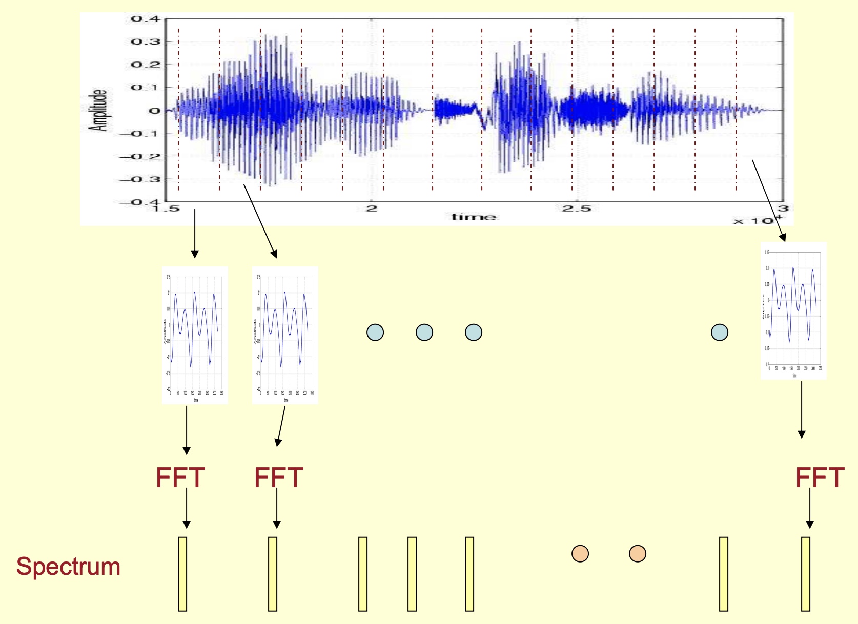
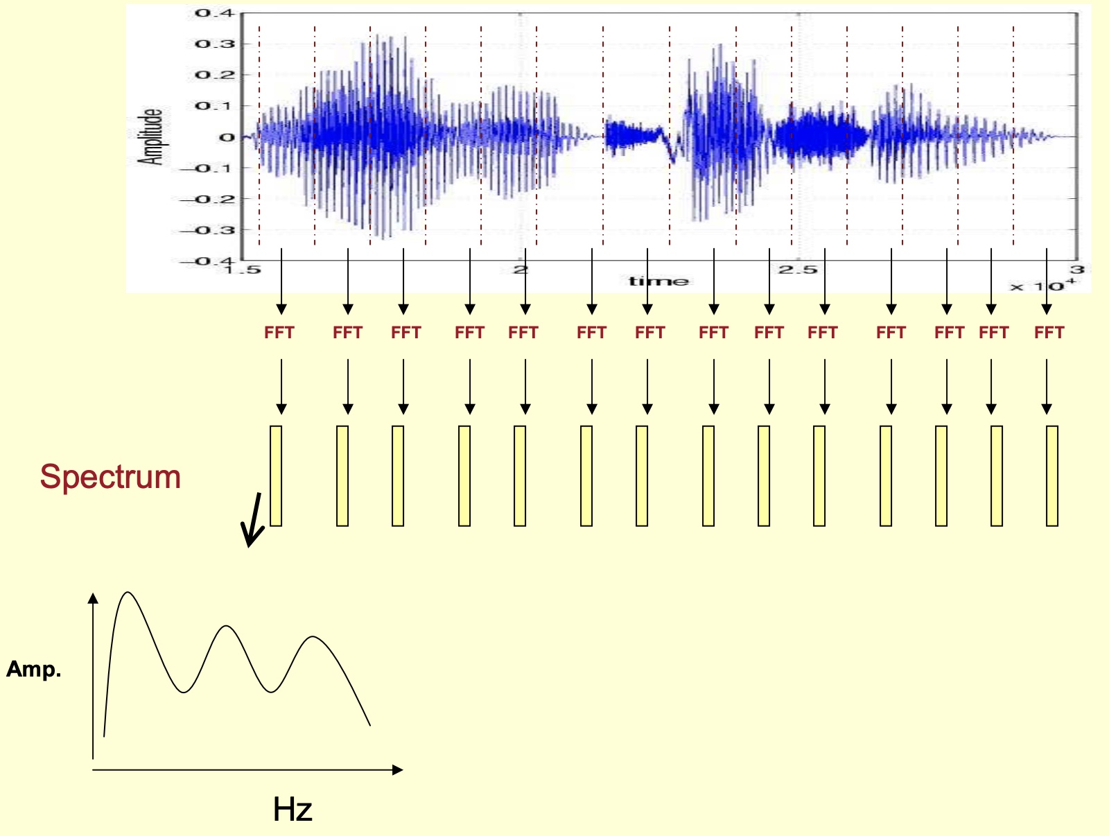
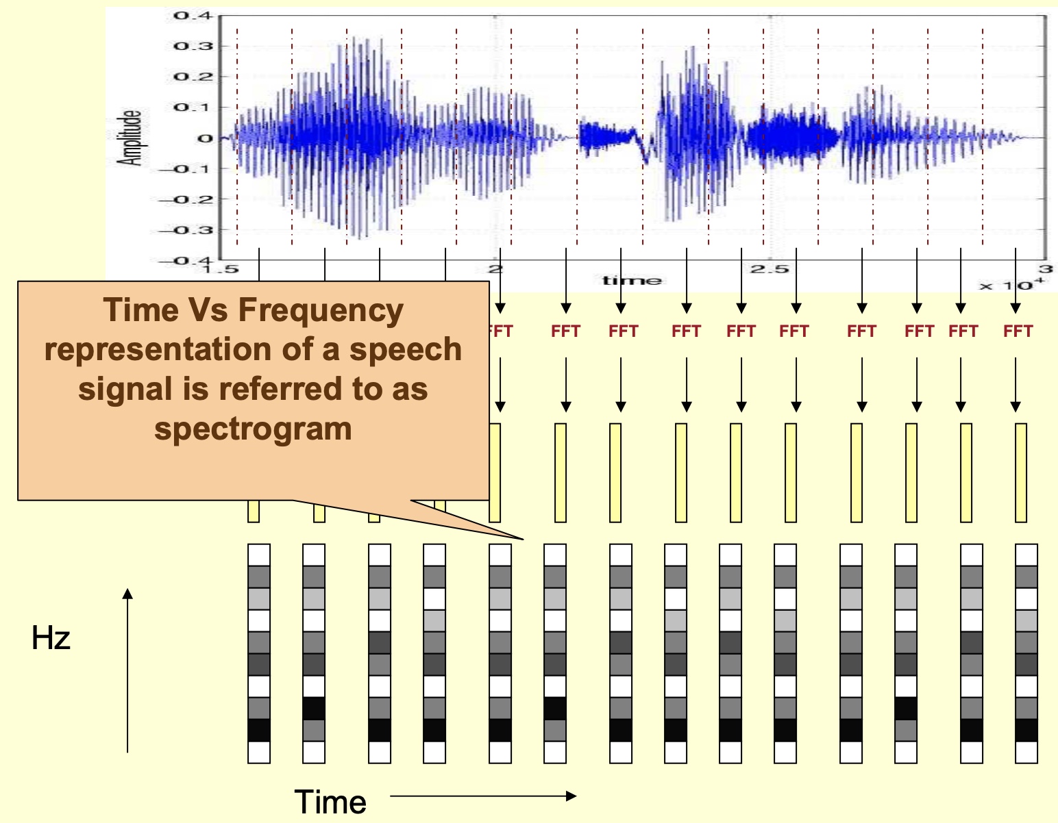
- Taking the Fourier transform of a slice of a speech signal yields the spectrum/spectral vector for that slice. A sequence of these spectral vectors yields the plot of frequency vs. time as shown below.
Spectrogram
- Frequency vs. time representation of a speech signal is referred to as a spectrogram.
- To obtain a spectrogram, first obtain the spectrum (image source: Speech Technology - Kishore Prahallad):
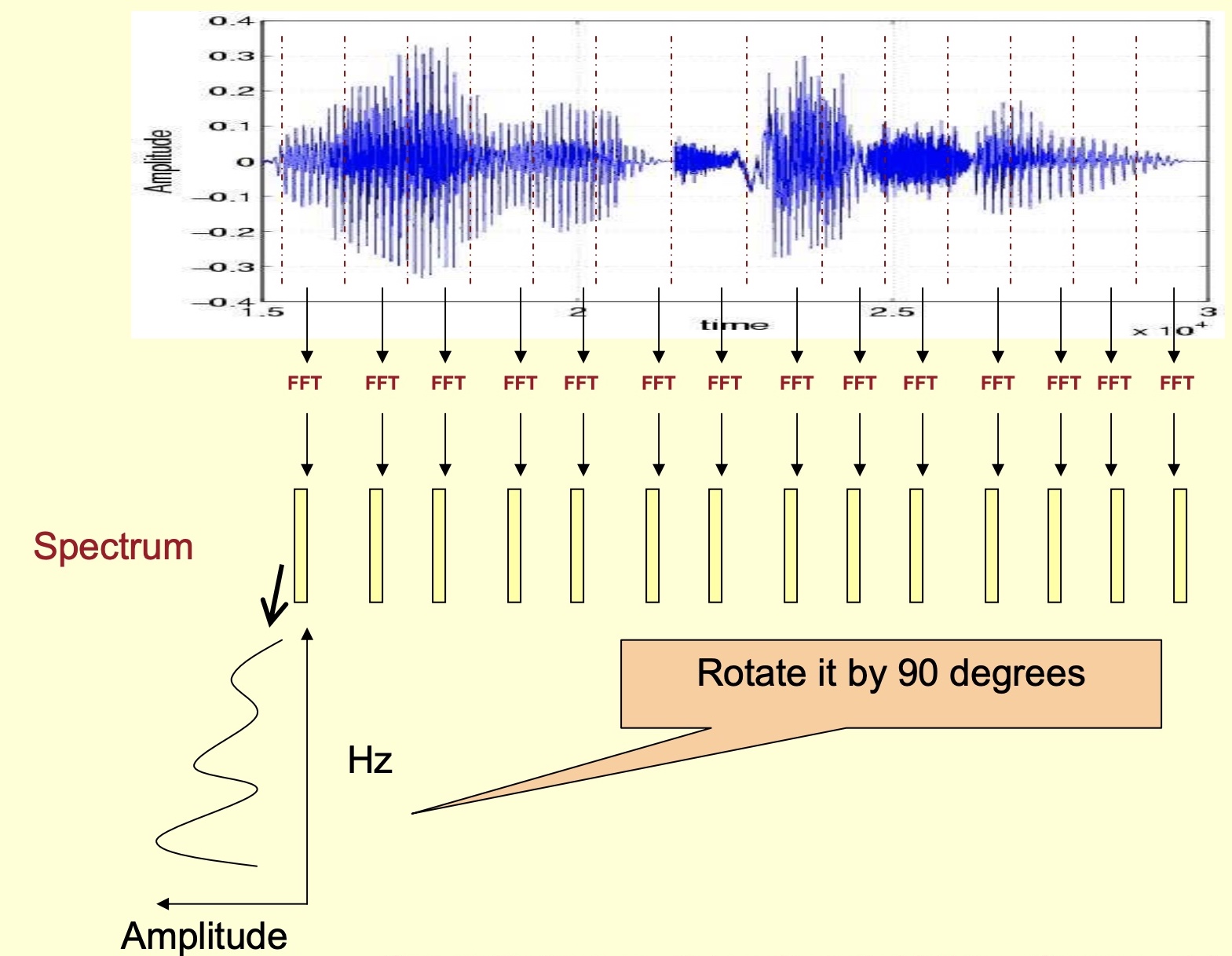
- Rotate it by 90 degrees:
- Color-code the amplitude:
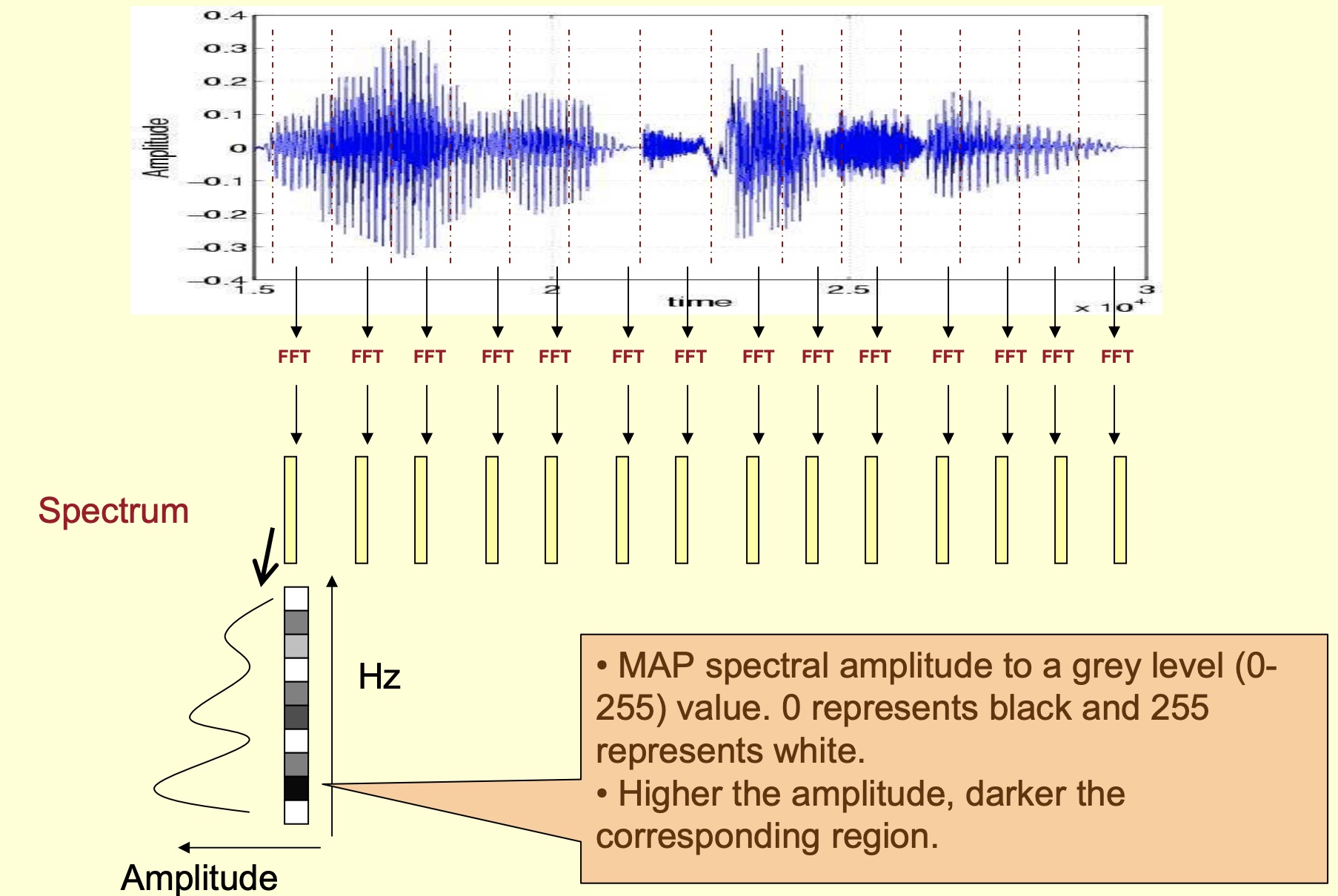
- Horizontally tiling the color-coded spectrums yields a spectrogram as shown below. A spectrogram is thus formally defined as a plot of frequency vs. time.
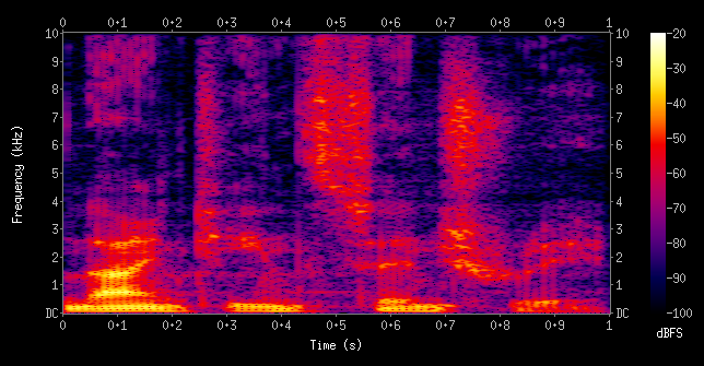
- An example spectrogram from Wikipedia: Spectrogram is as shown below:
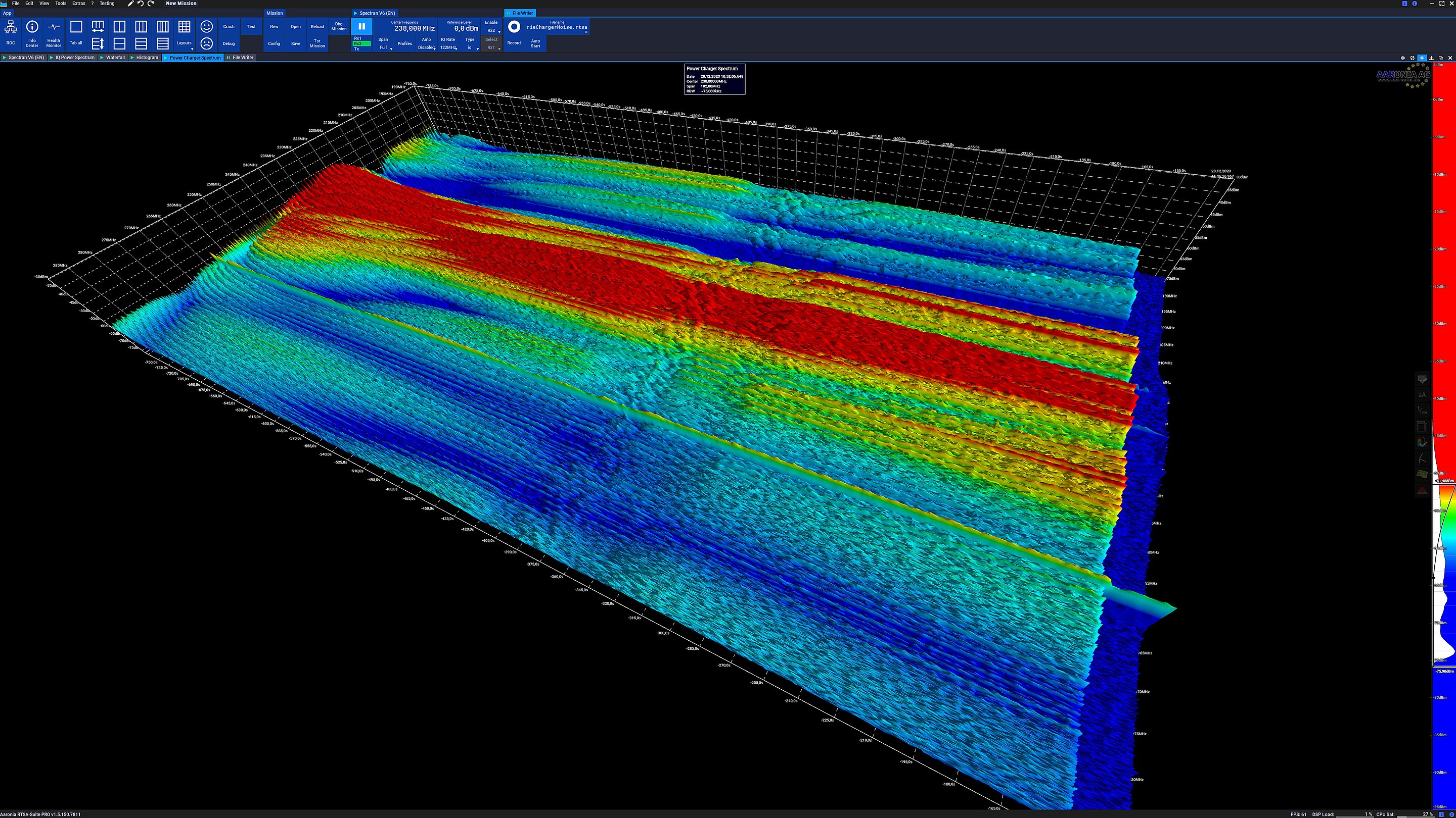
- An example 3D spectrogram is as shown below:
Why spectrograms?
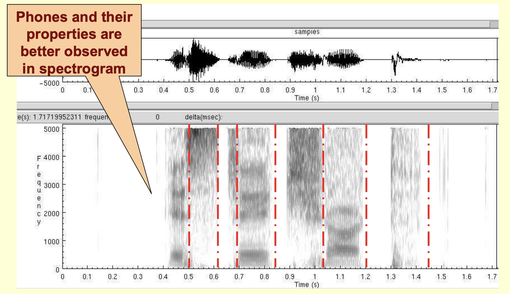
- Dark regions indicate peaks (formants) in the spectrum:
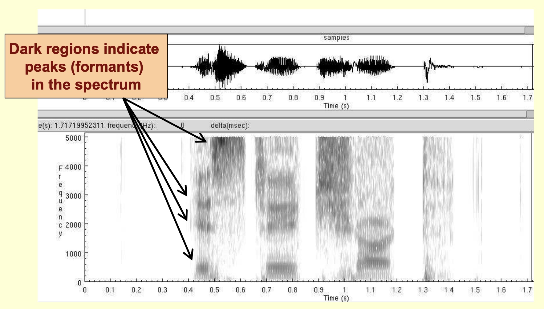
- Phones and their properties are better observed in spectrogram:
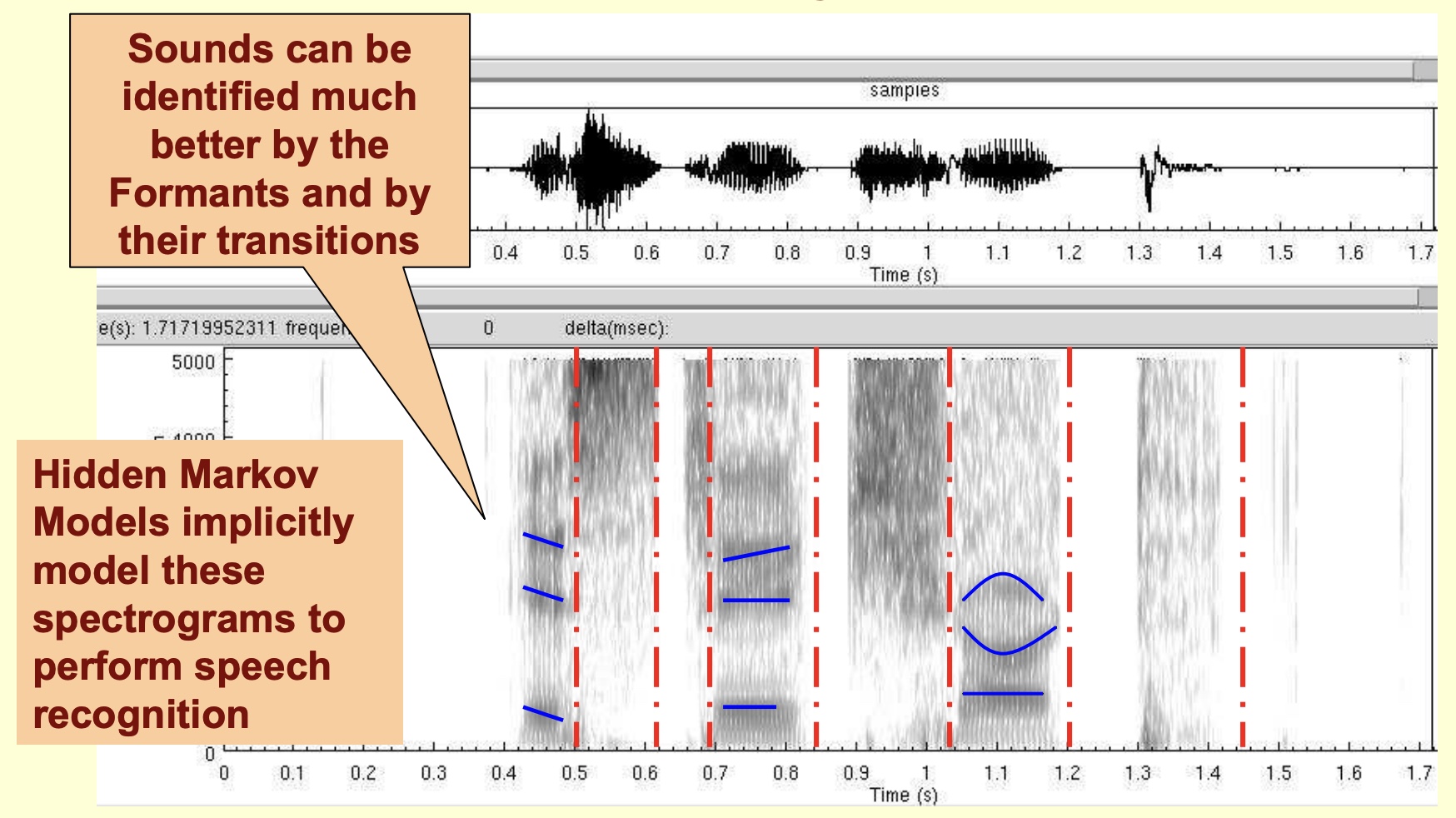
- Sounds can be identified much better by the formants and their transitions. Hidden Markov Models implicitly model these spectrograms to perform speech recognition.
- Key takeaways
- A spectrogram is a time-frequency representation of the speech signal.
- A spectrogram is a tool to study speech sounds (phones).
- Phones and their properties are visually studied by phoneticians using a spectrogram.
- Hidden Markov Models implicitly model spectrograms for speech to text systems.
- Useful for evaluation of text to speech systems: A high quality text to speech system should produce synthesized speech whose spectrograms nearly match those with with spoken language.
How are tokenizers used for pre-processing speech input?
-
Tokenizers are used for processing speech input in neural networks, especially in tasks like speech recognition, where the goal is to convert audio data into a textual format. These tokenizers in the context of speech processing work differently from those in text processing. Here’s a brief overview:
-
Feature Extraction: Before tokenization, the raw audio data is usually processed to extract meaningful features. Common features include spectrograms, Mel-frequency cepstral coefficients (MFCCs), or directly using raw waveform data. These features represent the audio in a more compact and informative way than raw waveforms.
-
Frame-Based Tokenization: The extracted features are often segmented into frames, which can be considered as tokens. Each frame captures a short segment of the audio signal (e.g., 20-30 milliseconds). This is similar to how text tokenization breaks down sentences into words or subwords.
-
Acoustic Modeling: These frames or tokens are then fed into an acoustic model, typically a neural network, which aims to map the audio features to a set of acoustic units. These units might be phonemes (basic units of sound), characters, or subword units.
-
Subword and Character Tokenizers: In some modern speech recognition systems, especially those based on end-to-end deep learning, subword or character tokenizers are used. These systems directly map the audio features to sequences of characters or subwords, bypassing the traditional phoneme-level representation. This approach has gained popularity with the advent of models like the Connectionist Temporal Classification (CTC) and attention-based models.
-
Byte Pair Encoding (BPE) and WordPiece: In advanced models, tokenizers like Byte Pair Encoding or WordPiece (common in NLP for text tokenization) are adapted for speech recognition. These methods dynamically create a vocabulary of common subword units based on the training data, which helps in handling a wide range of spoken language including rare words or names.
-
End-to-End Systems: In some end-to-end speech recognition systems, the concept of explicit tokenization is less clear. These systems take in raw audio and output text directly, using complex neural network architectures to implicitly handle the tokenization and recognition processes.
-
-
In summary, while the term “tokenizer” in speech processing might not always refer to a discrete component as in text processing, the concept of breaking down audio into manageable, meaningful units for further processing by neural networks is a fundamental part of modern speech recognition and processing systems.
What are “tokens” when embedding an audio sample using an encoder? How are they different compared to word/sub-word tokens in NLP?
- When embedding an audio sample using an encoder, especially in modern machine learning models, the concept of “tokens” is also applicable, albeit in a slightly different manner compared to text or image processing.
-
In the context of audio processing, particularly with neural network models, the audio signal is typically transformed into a series of numerical representations that can be analogously considered as “tokens.” Here’s how this process generally works:
-
Signal Segmentation: The continuous audio signal is first divided into smaller, manageable segments. This can be done using various methods such as windowing (e.g., short-time Fourier transform) or by directly splitting the raw waveform into chunks.
-
Feature Extraction: From each segment, features are extracted. These features can be in various forms, like Mel-frequency cepstral coefficients (MFCCs), spectrograms, or even raw audio waveforms. Each set of features represents a segment of the audio and can be thought of as an “audio token.”
-
Token Embeddings: These audio tokens are then transformed into a numerical format suitable for processing by a neural network. In some models, this might involve a linear transformation or the use of a more complex network like a convolutional neural network (CNN) to create a fixed-size vector, i.e., embeddings.
-
Sequence Processing: The resulting sequence of embeddings (tokens) is then fed into an encoder, such as a Transformer or a recurrent neural network (RNN), which processes the sequence to capture temporal relationships and patterns within the audio.
-
Positional Information: For models like Transformers, positional encodings might be added to the embeddings to provide temporal context, as Transformers do not inherently process sequential data in order.
-
- In the realm of advanced audio processing, such as in speech recognition, music generation, or audio classification, this approach of segmenting audio into tokens and processing them through neural networks has become increasingly common. It allows for capturing complex patterns and relationships in audio data, analogous to how text and images are processed in their respective domains.
Mel-Filterbanks and MFCCs
-
Empirical studies have shown that the human auditory system resolves frequencies non-linearly, and the non-linear resolution can be approximated using the Mel-scale which is given by
\[M(f)=1127.01048 \bullet \log _{e} f\]- where \(f\) is a frequency (Volkman, Stevens, & Newman, 1937).
- This indicates that the human auditory system is more sensitive to frequency difference in lower frequency band than in higher frequency band.
- The figure below illustrates the process of extracting Mel-frequency cepstrum coefficients (MFCCs) with triangular filters that are equally-spaced in Mel-scale. In the linear scale, note that as the frequency increases, the width of the filters increases.
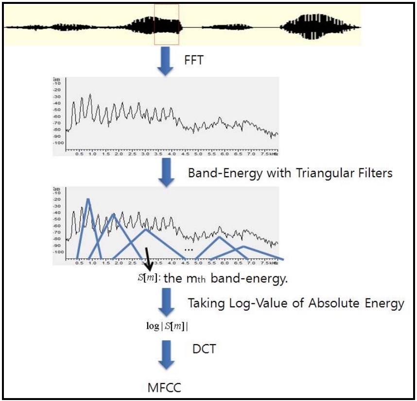
- An input speech is transformed using the Discrete Fourier Transform, and the filter-bank energies (also called the Mel filter-bank energies or Mel spectrogram) are computed using triangular filters mentioned above. The log-values of the filter-bank energies (also called the log-Mel filterbanks or log-Mel spectrogram) are then decorrelated using the discrete cosine transform (DCT). Finally, M-dimensional MFCCs are extracted by taking M-DCT coefficients, and passed on as speech features for downstream processing.
- However, deep learning models are able to exploit spectro-temporal correlations, enabling the use of the log-Mel spectrogram (instead of MFCCs) as equivalent or better options, especially as seen with tasks that involve automatic speech recognition (ASR) and keyword spotting (KWS). As a result, a good number of ASR and KWS papers utilize log-Mel or Mel filterbank speech features with temporal context.
- Research has reported that using MFCCs is beneficial for both speaker and speech recognition. While MFCCs are still commonly fed as input speech features to neural nets. However, newer neural net architectures typically rely on the log-Mel filterbank energies (LMFBE) (which can be used to generate MFCCs after DCT-based decorrelation as indicated above).
Example spectrogram and oscillogram
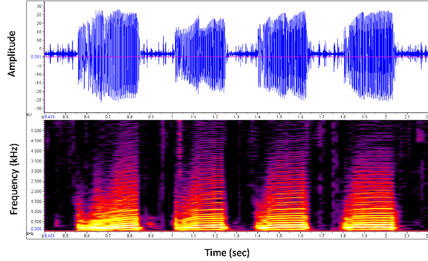
- This is an oscillogram and spectrogram of the boatwhistle call of the toadfish Sanopus astrifer. The upper blue-colored plot is an oscillogram presenting the waveform and amplitude of the sound over time, X-axis is Time (sec) and the Y-axis is Amplitude. The lower figure is a plot of the sounds’ frequency over time, X-axis is Time (sec) and the Y-axis is Frequency (kHz). The amount of energy present in each frequency is represented by the intensity of the color. The brighter the color, the more energy is present in the sound at that frequency.
Perceptual Linear Prediction (PLP)
- Similar from MFCCs, perceptual linear prediction (PLP) features can also be fed into neural nets as input. PLP is a combination of spectral analysis and linear prediction analysis. It uses concepts from the psychophysics of hearing to compute a simple auditory spectrum.
- Read more in H. Hermansky (1990).
Prosodic Features
- Prosodic features include pitch and its dynamic variations, inter-pause statistics, phone duration, etc. (Shriberg, 2007)
- Very often, prosodic features are extracted with larger frame size than acoustical features since prosodic features exist over a long speech segment such as syllables. The pitch and energy-contours change slowly compared to the spectrum, which implies that the variation can be captured over a long speech segment. Many pieces of literature have reported that prosodic features usually do not outperform acoustical features but incorporating prosodic features in addition to acoustical features can improve speaker recognition performance (Shriberg, 2007; Sönmez, Shriberg, Heck, & Weintraub, 1998; Peskin et al., 2003; Campbell, Reynolds, & Dunn, 2003; Reynolds et al., 2003).
Idiolectal Features
- The idiolectal features are motivated by the fact that people usually use idiolectal information to recognize speakers.
- In telephone conversation corpus, Doddington (2001) reported enrolled speakers can be verified not using acoustic features that are extracted from a speech signal but using idiolectal features that are observed in true-underlying transcription of speech. The phonetic speaker verification, motivated by Doddington (2001)’s work, creates a speaker using his/her phone n-gram probabilities that are obtained using multiple-language speech recognizers (Andrews, Kohler, & Campbell, 2001).
Speech Processing Tasks
Architectural overview
- A top-level overview of Siri architecture from Deep Learning in Speech Recognition by Alex Acero, Apple Inc. is shown below.
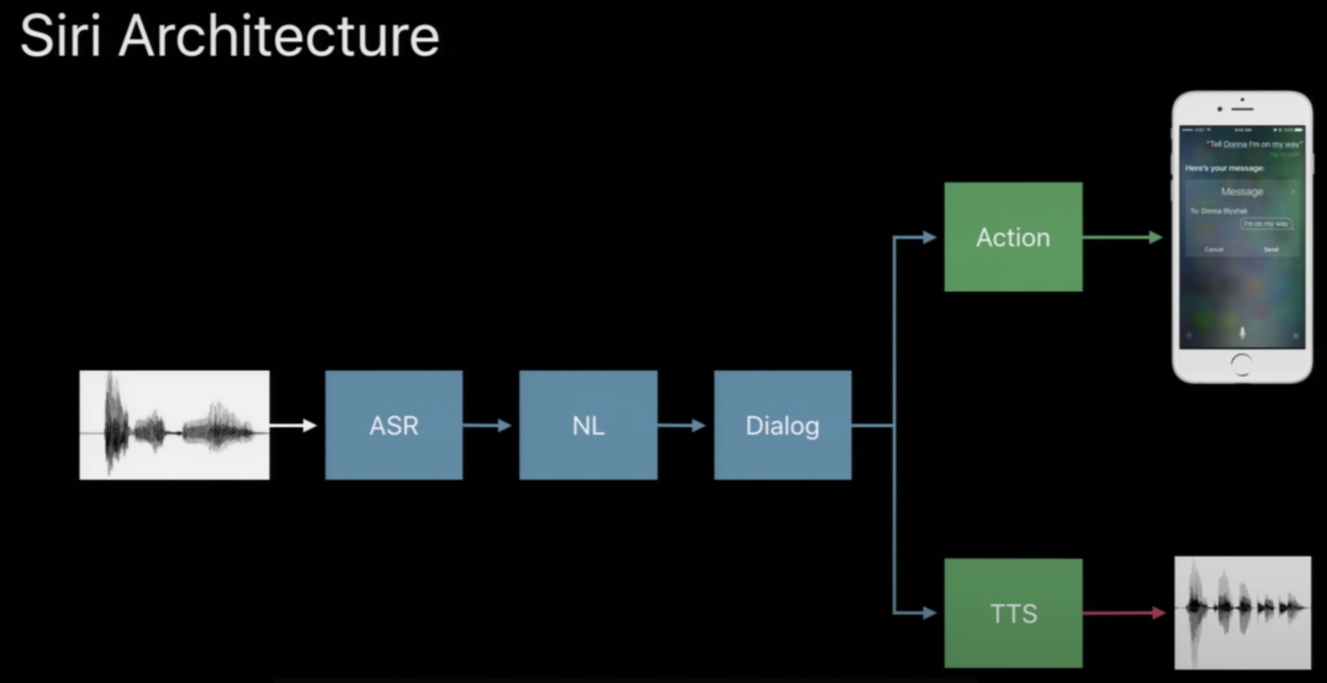
- Note that this is an oversimplification of a complex system. Usually, the input data (which is pre-processed into speech features such as Mel-Filterbanks or MFCCs) gets fed as an input to the keyword spotting module which further gates two modules: (i) speaker recognition module, and (ii) automatic speech recognition (ASR) module. The encoder part of the ASR module can run in parallel with a language identification (LID) module which can select the language model correspond to the detected language which feeds the ASR decoder. The ASR output further feeds the natural language understanding (NLU) block which performs intent classification and slot filling. Dialog acts are generated next. Finally, the text-to-speech synthesis (TTS) block yields the end result: a response from the voice assistant. Note that the detected language also helps select which NLU and TTS block to use.
- Also note that the first phase of the above flow, keyword spotting, can be gated by a voice activity detector (VAD) which is usually a simple neural network with a couple of layers whose job is to just figure out if there’s speech or not in the audio it is listening to. This is usually an always-on on-device block. This helps save power by not having a more complex model like the keyword spotter run as an always-on system.
Fundamental speech tasks
- There four fundamental speech tasks, as applied to digital voice assistants:
- Wake word detection/keyword spotting (KWS): On the device, detect the wakeword/trigger keyword to get the device’s attention;
- Automatic speech recognition (ASR): Upon detecting the wake word, convert audio streamed to the cloud into words;
- Natural-language understanding (NLU): Extract the meaning of the recognized words so that the assistant can take the appropriate action in response to the customer’s request; and
- Text-to-speech synthesis (TTS): Convert the assistant’s textual response to the customer’s request into spoken audio.
Hierarchy of phones, words, and sentences
-
The input audio (typically stored as a wave-file, but could be another audio format as well, such as FLACC, OGG, etc.) is converted to a feature sequence \((f_1, \ldots, f_T)\). The goal is to find a sequence of words \((w_1, \ldots, w_N)\) that matches the feature sequence best.
-
An HMM is used to model basic units (phones) in speech. To bridge the gap between phone-level HMMs and word decoding, let’s look at the hierarchical structure of HMM states, phones, words and sentences.
- A phone is usually modeled by a HMM with three states. The three states correspond to three subphones, which are transition-in, steady-state, transition-out regions of the phone.
- A word is consisted by a sequence of phones. For example, “one” is composed of three phones:
w,ah, andn. The word model is just the sequential concatenation of the phone models. - Lexicon contains information about phone sequence of words. There is a dictionary (lexicon) which includes phone sequence for each of word. Therefore once all phones are represented by pre-trained HMM models, the word models become available by searching in the dictionary and concatenating phone level models belonging to that word. Compared with fitting a HMM for individual word, this strategy greatly reduced the complexity.
- A sentence is a grammatically valid sequence of words. Words do not randomly connect to form a sentence. The transition between adjacent words can be estimated from a large text corpus.
Automatic Speech Recognition
What is automatic speech recognition?
- Research in ASR (Automatic Speech Recognition) aims to enable computers to “understand” human speech and convert it into text. ASR is the next frontier in intelligent human-machine interaction and also a precondition for perfecting machine translation and natural language understanding. Research into ASR can be traced back to the 1950s in its initial isolated word speech recognition system. Since then, with persistent efforts of numerous scholars, ASR has made significant progress and can now power large-vocabulary continuous speech recognition systems.
- Especially in the emerging era of big data and application of deep neural networks, ASR systems have achieved notable performance improvements. ASR technology has also been gradually gaining practical use, becoming more product-oriented. Smart speech recognition software and applications based on ASR are increasingly entering our daily lives, in form of voice input methods, intelligent voice assistants, and interactive voice recognition systems for vehicles.
Framework of an ASR System
-
The purpose of ASR is to map input waveform sequences to their corresponding word or character sequences. Therefore, implementing ASR can be considered a channel decoding or pattern classification problem. Statistical modeling is a core ASR method, in which, for a given speech waveform sequence \(O\), we can use a “maximum a posteriori” (MAP) estimator, based on the mode of a posterior Bayesian distribution, to estimate the most likely output sequence \(W*\), with the formula shown in the figure below.
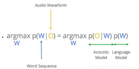
- where, \(P(O \mid W)\) is the probability of generating the correct observation sequence, i.e. corresponding to the acoustic model (AM) of the ASR system, conditional on \(W\). Likelihood \(P(W)\) is the ‘a priori probability’ of the exact sequence \(W\) occurring. It is called the language model (LM).
-
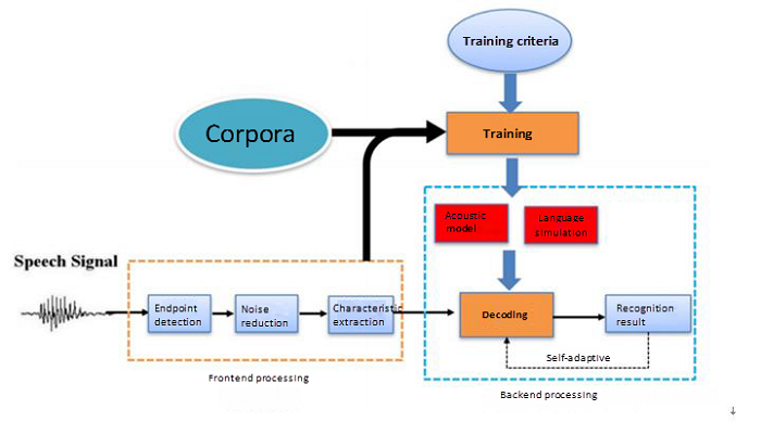
The figure below shows the structure diagram of a marked ASR system, which mainly comprises a front-end processing module, acoustic model, language model, and decoder. The decoding process is primarily to use the trained acoustic model and language model to obtain the optimal output sequence.
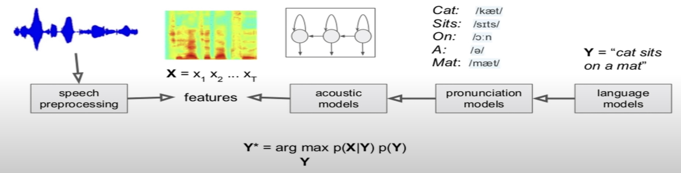
- A version of the ASR system (with components such as pronunciation models, language models for re-scoring) from End-to-End Models for Speech Processing at Stanford by Navdeep Jaitly, NVIDIA is as below:
Acoustic Model (Encoder)
- An acoustic model’s task is to compute \(P(O \mid W)\), i.e. the probability of generating a speech waveform for the mode. An acoustic model, as an important part of the ASR system, accounts for a large part of the computational overhead and also determines the system’s performance. GMM-HMM-based acoustic models are widely used in traditional speech recognition systems.
- In this model, GMM is used to model the distribution of the acoustic characteristics of speech and HMM is used to model the time sequence of speech signals. Since the rise of deep learning in 2006, deep neural networks (DNNs) have been applied in speech acoustic models. In Mohamed et al. (2009), Hinton and his students used feedforward fully-connected deep neural networks in speech recognition acoustic modeling.
- Typical pre-processing involves converting the audio to mono (similar to how computer vision models flatten the input image across the three channels, viz., R, G, B) and resampling it to 16kHz before it is input to the model.
Encoder-Decoder Architectures: Past vs. Present
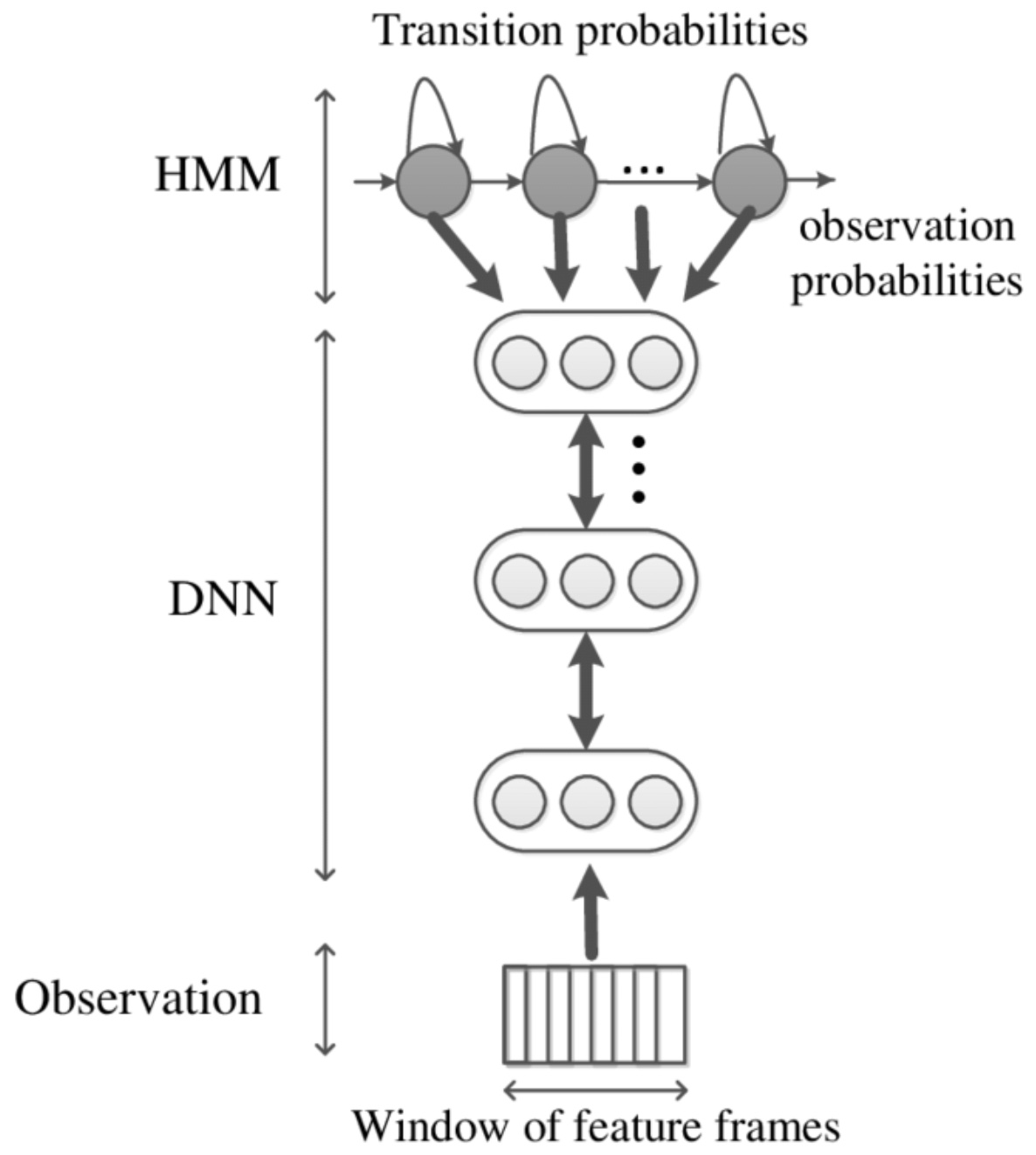
- Traditional speech recognition systems adopt a GMM-HMM architecture where the GMM is the acoustic model that computes the state/observation probabilities and the HMM decoder combines these probabilities using dynamic programming (DP). With the advent of deep learning, the role played by the GMM as the acoustic model is now replaced by a DNN. Rather than the GMM modeling the observation probabilities, a DNN is trained to output them. The HMM still acts as a decoder. The figure below illustrates both approaches side-by-side.
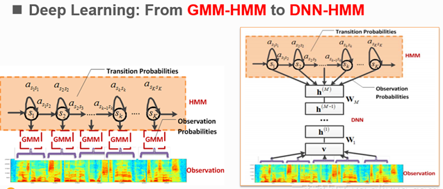
- The DNN computes the observation probabilities and outputs a probability distribution over as many classes as the HMM states for each speech frame using a softmax layer. The number of HMM states depend of the number of phones, with a typical setup of 3 target labels for each phone for the beginning, middle and end of the segment, 1 state for silence, and 1 state for background. The DNN is typically trained to minimize the average cross-entropy loss over all frames between the predicted and the ground-truth distributions. The HMM decoder computes the word detection score using the observation, the state transition, and the prior probabilities. An architectural overview of a DNN-HMM is shown in the diagram below.
- Compared to traditional GMM-HMM acoustic models, DNN-HMM-based acoustic models perform better in terms of TIMIT database. When compared with GMM, DNN is advantageous in the following ways:
- De-distribution hypothesis is not required for characteristic distribution when DNN models the posterior probability of the acoustic characteristics of speech.
- GMM requires de-correlation processing for input characteristics, but DNN is capable of using various forms of input characteristics.
- GMM can only use single-frame speech as inputs, but DNN is capable of capturing valid context information by means of splicing adjoining frames.
- Once the HMM model is built, to figure out the maximum a posteriori probability estimate of the most likely sequence of hidden states, i.e., the Viterbi path, a graph-traversal algorithm like the Viterbi decoder algorithm (typically implemented using the concept of dynamic programming in algorithms) can be applied.
- Given that speech comprises of sequential data, RNNs (and it’s variants, GRUs and LSTMs) are natural choices for DNNs. However, for tasks such as speech recognition, where the alignment between the inputs and the labels is unknown, RNNs have so far been limited to an auxiliary role. The problem is that the standard training methods require a separate target for every input, which is usually not available. The traditional solution — the so-called hybrid approach — is to use Hidden Markov Models (HMMs) to generate targets for the RNN, then invert the RNN outputs to provide observation probabilities (Bourlard and Morgan, 1994). However the hybrid approach does not exploit the full potential of RNNs for sequence processing, and it also leads to an awkward combination of discriminative and generative training.
- The connectionist temporal classification (CTC) output layer (Graves et al., 2006) removes the need for HMMs for providing alignment altogether by directly training RNNs to label sequences with unknown alignments, using a single discriminative loss function. CTC can also be combined with probabilistic language models for word-level speech and handwriting recognition. Note that the HMM-based decoder is still a good idea for cases where the task at hand involves a limited vocabulary and as a result, a smaller set of pronunciations, such as keyword spotting (vs. speech recognition).
- Using the CTC loss enables all-neural encoder-decoder seq2seq architectures that utilize an end-to-end neural architecture which generates phonemes at the output of the encoder as an intermediate step, which are consumed by a decoder which utilizes a language model and pronunciation model to generate transcriptions. The language model helps with secondary aspects of ASR such as punctuation, capitalization, and suggesting the right spellings based on the best word match.
- Recent models in this area such as Listen Attend Spell (LAS) forgo the intermediate phoneme labels altogether and train an end-to-end architecture that directly emits transcriptions at its output.
- For more in this area, Alex Graves’s book on Supervised Sequence Labelling with Recurrent Neural Networks is a great reference.
Putting it all together
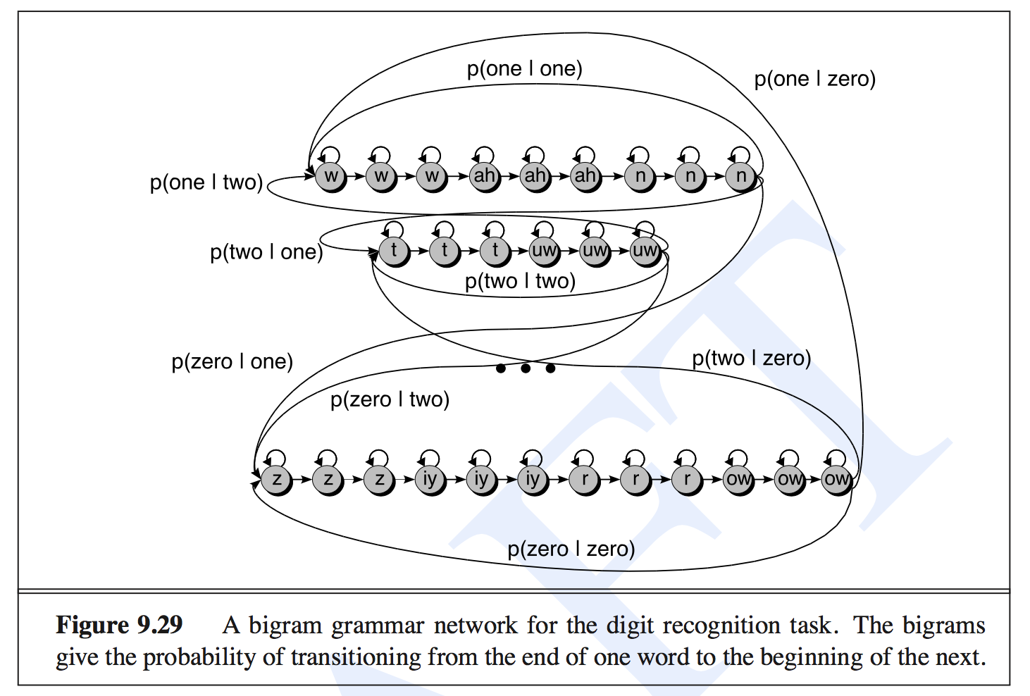
- Let’s take an example of a simple digit recognition task. The words are the digits from one to nine. THe following hierarchical graph from Speech and Language Processing by Jurafsky and Martin, 2008 shows the hierarchical transitions of this task. \(P(one \| two)\) represents the transition probability from digit two to one.
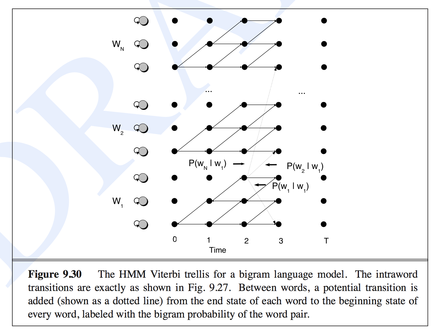
- Given this hierarchical transition matrix, a Viterbi trellis decoding method is used. The following figure from Speech and Language Processing by Jurafsky and Martin, 2008 shows the scheme of this decoding process. The words (digits) are stacked vertically and the feature sequence is shown horizontally.
Keyword Spotting / Wakeword Detection
- To achieve always-on keyword spotting, running a complex neural network all the time is a recipe for battery drain.
- The trick is to use a two-pass system by breaking down the problem into two pieces: (i) low-compute (running on an always-on processor), and (ii) more accurate (running on the main processor) as shown below:
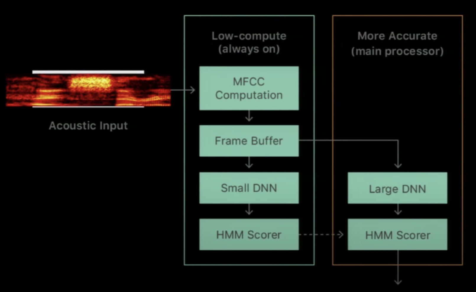
- The first low-compute piece typically runs on a special always-on processor (AOP) which is named so because it does not enter sleep states (unlike the main processor) and is always-on. The trade-off is that it is much less powerful than the main processor so you can only do small number of computations if you don’t want to impact the battery life.
- The second more accurate piece running on the main processor consumes high power but only uses that power for a very limited amount of time when you actually want it to compute something, i.e., when it is not sleeping. The rest of the time it goes to several levels of sleep and most of the time the main processor is completely asleep.
- Thus, we have a two layer system similar to a processor cache hierarchy. The first level is running all the time with a very simple DNN and then if it is confident with its predictions, it does not wake up the main system. However, if it is unsure of its predictions, it wakes up the main processor which runs a bigger, fancier DNN that is more accurate.
- Note that both passes share the same set of computed speech features which are typically generated on the AOP.
- The level-1/first-stage thresholds are tuned to trade-off false-reject rates for high false-accept rates so we don’t easily miss an event where the user was looking to interact with the device due to it not waking up the second-stage (negatives/rejects do not wake up stage-2). Since the level-2/second-stage model is a beefier model, it can mitigate false-accepts easily. It is also important to make sure the precision is not too low as to wake up the level-2/second-stage model (also known as the “checker” model) frequently, and eventually lead to a battery drain.
- This requires the level-1 stage to have high recall with modest precision to ensure that the voice assistant doesn’t miss a true positive. At the same time, the level-1 stage needs to optimize for speed to ensure we deliver a great set of candidates and satisfy the strict latency requirements of the system.
- The level-2 stage, on the other hand, has high precision with modest recall to ensure a smooth user-experience by ensuring that the voice-assistant minimizes false positives (and avoids waking up frequently due to excessive false positives). The level-2 stage can also incorporate a more complex architecture; since the level-2 stage is only invoked on a handful of instances compared to level-1, the latencies involved with such complex architectures are usually manageable.
- This paradigm is similar to how recommender systems optimize for recall during their retrieval stage and precision during their ranking stage.
Measuring Performance
- Evaluating performance in keyword spotting involves several key metrics, primarily focusing on Precision, Recall, F1-score, and Detection Error Trade-off (DET) curves. Each metric provides a distinct perspective on the system’s performance and effectiveness in different operational scenarios.
Precision
- Precision measures the accuracy of the model in identifying wakewords. It indicates how many of the model’s wakeword detections are correct, calculated as:
- A high precision value ensures fewer false activations, conserving device power and enhancing user experience by reducing unintended interactions.
Recall
- Recall assesses the reliability of the model in detecting actual wakeword occurrences. It shows the proportion of actual wakeword instances the model successfully identifies, calculated as:
- High recall ensures the voice assistant is consistently responsive, minimizing missed interactions and improving user satisfaction.
Precision-Recall (PR) Curves
- Precision-Recall curves visually illustrate the trade-off between precision and recall at various threshold settings. By plotting precision against recall, developers can analyze system behavior and select optimal operational thresholds that suit specific precision and recall requirements.
- However, PR curves have limitations in keyword spotting scenarios, especially when evaluating systems where false positives and false negatives must both be strictly managed.
F1-score
- The F1-score provides a balanced evaluation by combining precision and recall into a single metric. It is especially useful in scenarios where balancing false positives and false negatives is critical. The F1-score is the harmonic mean of precision and recall:
- Optimizing the F1-score helps maintain a balanced performance between accuracy and reliability.
Detection Error Trade-off (DET) Curves
-
DET curves offer a comprehensive visual assessment of keyword spotting system performance, particularly highlighting the trade-offs between false alarm rates and missed detection rates across varying thresholds. Unlike precision-recall curves, DET curves specifically plot the False Negative Rate (FNR) against the False Positive Rate (FPR) on a normal deviate scale.
-
False Negative Rate (FNR): Probability of missing the wakeword (i.e., not waking the device when the wakeword is spoken), calculated as:
- False Positive Rate (FPR): Probability of falsely detecting a wakeword when it is not present, calculated as:
-
DET curves are generally preferred for keyword spotting tasks due to several advantages:
- Symmetric Visualization: DET curves equally emphasize both false positives and false negatives, enabling balanced optimization.
- Clear Operational Trade-offs: DET curves provide a clearer depiction of trade-offs critical for user experience and battery efficiency.
- Direct Threshold Selection: They facilitate intuitive threshold tuning aligned with real-world performance requirements, directly addressing operational priorities.
-
By employing DET curves alongside precision, recall, and F1-score, developers can holistically assess and optimize keyword spotting systems, ensuring effective balance across responsiveness, accuracy, and power efficiency.
Online learning with live data to improve robustness
- To improve the robustness of a speech model such as ASR, Keyword Spotting etc., we can train it on online data gathered from the field. To do so, we run the classifier with a very low threshold, for instance, in case of keyword spotting, if the usual detection threshold is 0.8, we run it at a threshold of 0.5. This leads to the keyword spotter firing on a lot of keywords – most of them being false positives and the others being true positives. This is because for a classifier, lower the classification threshold, more the number of false positives, while higher the classification threshold, more the number of false negatives.
- Next, we manually sift through the results and identify the true positives and use them for re-training the classifier. The false positives, in turn, are used as hard negatives to also re-train the classifier and thus, make it more robust to erroneous scenarios involving false accepts.
Handling dynamic language switching and code switching
- In order to support such dynamic language switching from one interaction to the next (which is different from code switching, where words from more than one language are used within the same interaction or utterance), the backend intelligence must perform language identification (LID) along with automatic speech recognition (ASR) so that the detected language can be used to trigger appropriate downstream systems such as natural language understanding, text-to-speech synthesis, etc., which usually are language specific.
- To enable dynamic language switching between two or more pre-specified languages, a commonly adopted strategy is to run several monolingual ASR systems in parallel along with a standalone acoustic LID module, and pass only one of the recognized transcripts downstream depending on the outcome of language detection. While this approach works well in practice, it is neither cost-effective for more than two languages, nor suitable for on-device scenarios where compute resources and memory are limited. To this end, Joint ASR and Language Identification Using RNN-T: An Efficient Approach to Dynamic Language Switching (2021) proposed all-neural architectures that can jointly perform ASR and LID for a group of pre-specified languages and thereby significantly improve the cost effectiveness and efficiency of dynamic language switching. Joint ASR-LID modeling, by definition, involves multilingual speech recognition. Multilingual ASR models are trained by pooling data from the languages of interest, and it is often observed that languages with smaller amounts of data (i.e., low-resource languages) benefit more from this.
Speaker Recognition
- Speaker recognition can be classified into (i) speaker verification, and (ii) speaker identification. Speaker verification aims to verify whether an input speech corresponds to the claimed identity. Speaker identification aims to identify an input speech by selecting one model from a set of enrolled speaker models. In some cases, speaker verification follows speaker identification in order to validate the identification result.
- Speaker verification is gauged using the EER metric on the DET-curve while speaker identification is gauged using accuracy.
- i-vectors by Dehak et al. in 2010 were the leading technology behind speaker recognition, up until DNNs took over with d-vectors by Variani et al. in 2014. The latest in speaker recognition is x-vectors by Snyder et al. in 2018 which proposed using data augmentation, consisting of added noise and reverberation, as an inexpensive method to multiply the amount of training data and improve robustness. The figure below shows the embedding extraction process with d-vectors:
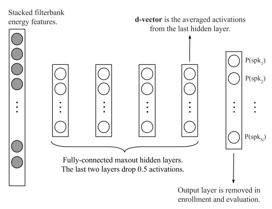
- Read more on speaker recognition in this book chapter by Jin and Yoo from KAIST.
Data augmentation
Time domain
Gain
- Gain augmentation can be applied by simply multiplying the raw audio by a scalar.
Types of noise
Reverberation noise / room impulse response (RIR)
- Reverberation noise, also known as room impulse response (RIR), is produced when a sound source stops within an enclosed space. Sound waves continue to reflect off the ceiling, walls and floor surfaces until they eventually die out. These reflected sound waves are known as reverberation.
Babble noise
- Babble noise is considered as one of the best noises for masking speech. Refer Babble Noise: Modeling, Analysis, and Applications.
Speed and pitch
- These augmentations, while slow to run, are mainly used to artificially increase the number of training speakers.
Codec augmentation
- Transcoding audio in a new codec can increase diversity in the training dataset, however it is extremely slow and we expect Alexa data to have limited variation in used codecs.
Mixup
- Mixup has shown promising results on small datasets with a limited number of utterances per training speaker.
Dynamic Range Compression
- We do expect most Alexa recordings to have a constant volume due to the audio preprocessing. Therefore we expect that introducing or suppressing volume variations within a recording to have a limited impact on real world data.
Frequency domain
SpecAugment
- This paper by Park et al. (2019) from Google presents SpecAugment, a simple data augmentation method for speech recognition.
- SpecAugment greatly improves the performance of ASR networks. SpecAugment is applied directly to the feature inputs of a neural network (i.e., filter bank coefficients). The augmentation policy consists of warping the features, masking blocks of frequency channels, and masking blocks of time steps. They apply SpecAugment on Listen, Attend and Spell (LAS) networks for end-to-end speech recognition tasks.
- They achieve state-of-the-art performance on the LibriSpeech 960h and Swichboard 300h tasks on end-to-end LAS networks by augmenting the training set using simple handcrafted policies, surpassing the performance of hybrid systems even without the aid of a language model. SpecAugment converts ASR from an over-fitting to an under-fitting problem, and they are able to gain performance by using bigger networks and training longer. On LibriSpeech, they achieve 6.8% WER (more on WER in the section on Evaluation metrics) on test-other without the use of a language model, and 5.8% WER with shallow fusion with a language model. This compares to the previous state-of-the-art hybrid system of 7.5% WER. For Switchboard, they achieve 7.2%/14.6% on the Switchboard/CallHome portion of the Hub5’00 test set without the use of a language model, and 6.8%/14.1% with shallow fusion, which compares to the previous state-of-the-art hybrid system at 8.3%/17.3% WER.
Evaluation metrics
Precision and Recall
- In case of an imbalanced dataset scenario, precision and recall are appropriate performance metrics. Precision and recall are typically juxtaposed together when reported.
- Precision is defined as the fraction of relevant instances among all retrieved instances.
- Recall, sometimes referred to as sensitivity, is the fraction of retrieved instances among all relevant instances.
- Note that precision and recall are computed for each class. They are commonly used to evaluate the performance of classification or information retrieval systems.
A perfect classifier has precision and recall both equal to 1.
- It is often possible to calibrate the number of results returned by a model and improve precision at the expense of recall, or vice versa.
- Precision and recall should always be reported together and are not quoted individually. This is because it is easy to vary the sensitivity of a model to improve precision at the expense of recall, or vice versa.
- As an example, imagine that the manufacturer of a pregnancy test needed to reach a certain level of precision, or of specificity, for FDA approval. The pregnancy test shows one line if it is moderately confident of the pregnancy, and a double line if it is very sure. If the manufacturer decides to only count the double lines as positives, the test will return far fewer positives overall, but the precision will improve, while the recall will go down. This shows why precision and recall should always be reported together.
- The figure below (taken from the Wikipedia article on precision and recall) shows a graphical representation of precision and recall:
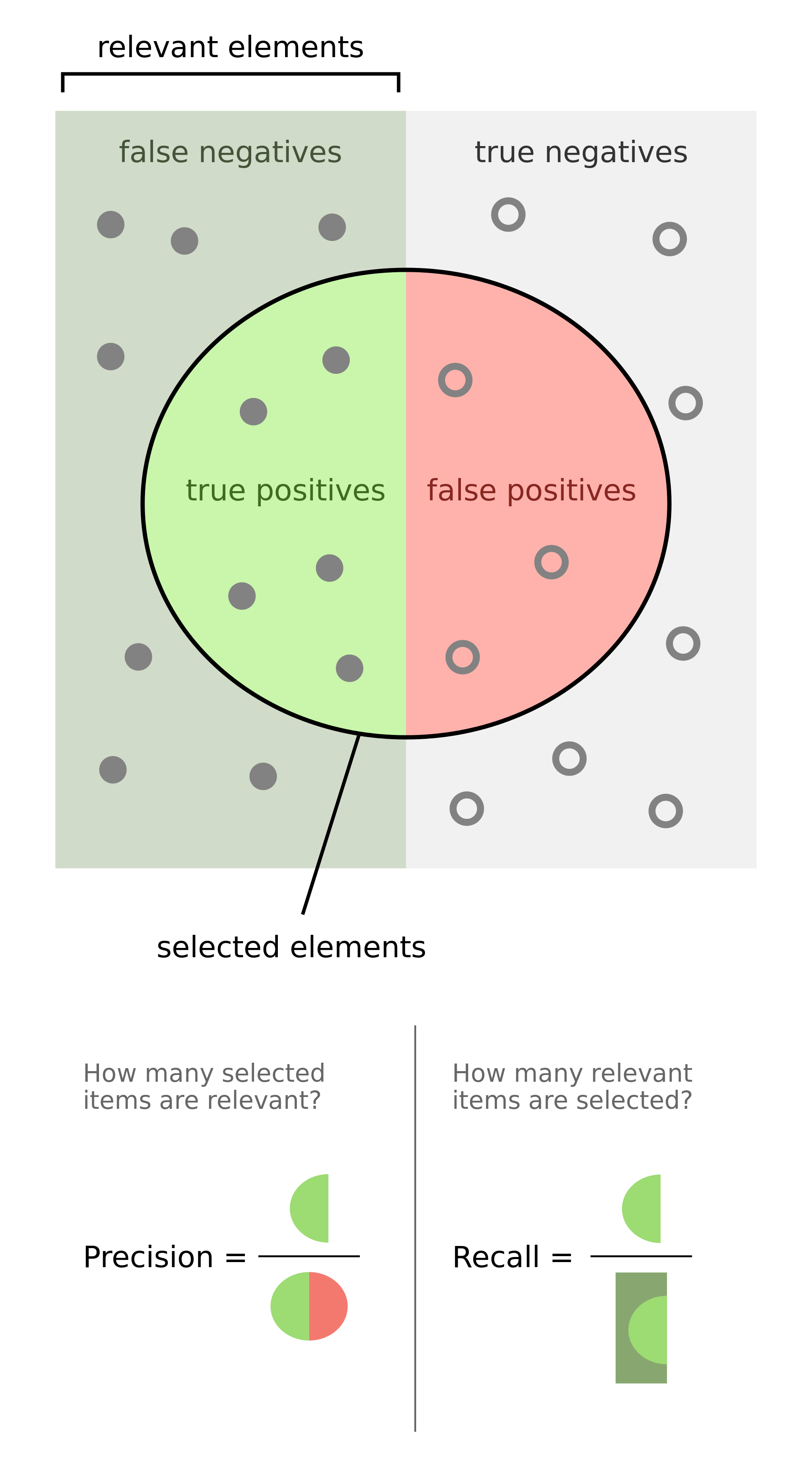
- Formally, precision and recall can be defined as:
- Precision: Out of all the samples marked positive, how many were actually positive (i.e., the true positives)?
- Recall: Out of all the samples that are actually positive, how many were marked positive (i.e., the true positives)?
- From the above definitions it is clear that with PR metrics, the focus is on the positive class (also called the relevant class).
-
In the section on Precision-Recall (PR) Curves, we explore how to get the best out of these two metrics using PR curves.
- Key takeaways
- Precision: how many selected items are relevant?
- Recall: how many relevant items are selected?
Historical Background
- This section is optional and offers a historical walk-through of how precision, recall and F1-score came about, so you may skip to the next section if so desired.
- Precision and recall were first defined by the American scientist Allen Kent and his colleagues in their 1955 paper Machine literature searching VIII. Operational criteria for designing information retrieval systems.
- Kent served in the US Army Air Corps in World War II, and was assigned after the war by the US military to a classified project at MIT in mechanized document encoding and search.
- In 1955, Kent and his colleagues Madeline Berry, Fred Luehrs, and J.W. Perry were working on a project in information retrieval using punch cards and reel-to-reel tapes. The team found a need to be able to quantify the performance of an information retrieval system objectively, allowing improvements in a system to be measured consistently, and so they published their definition of precision and recall.
- They described their ideas as a theory underlying the field of information retrieval, just as the second law of thermodynamics “underlies the design of a steam engine, regardless of its type or power rating”.
- Since then, the definitions of precision and recall have remained fundamentally the same, although for search engines the definitions have been modified to take into account certain nuances of human behavior, giving rise to the modified metrics precision @ \(k\) and mean average precision (mAP), which are the values normally quoted in information retrieval contexts today.
- In 1979, the Dutch computer science professor Cornelis Joost van Rijsbergen recognized the problems of defining search engine performance in terms of two numbers and decided on a convenient scalar function that combines the two. He called this metric the Effectiveness function and assigned it the letter E. This was later modified to the \(F_1\) score, or \(F_{\beta}\) score, which is still used today to summarize precision and recall.
Examples
- Precision and recall can be best explained using examples. Consider the case of evaluating how well does a robot sifts good apples from rotten apples. A robot looks into the basket and picks out all the good apples, leaving the rotten apples behind, but is not perfect and could sometimes mistake a rotten apple for a good apple orange.
- After the robot finishes picking the good apples, precision and recall can be calculated as:
- Precision: number of good apples picked out of all the picked apples.
- Recall: number of good apples picked out of all possible good apples.
- Precision is about exactness, classifying only one instance correctly yields 100% precision, but a very low recall, it tells us how well the system identifies samples from a given class.
- Recall is about completeness, classifying all instances as positive yields 100% recall, but a very low precision, it tells how well the system does and identify all the samples from a given class.
- As another example, consider the task of information retrieval. As such, precision and recall can be calculated as:
- Precision: number of relevant documents retrieved out of all retrieved documents.
- Recall: number of relevant documents retrieved out of all relevant documents.
Applications
- Precision and recall are measured for every possible class in your dataset. So, precision and recall metrics are relatively much more appropriate (especially compared to accuracy) when dealing with imbalanced classes.
An important point to note is that PR are able to handle class imbalance in scenarios where the positive class (also called the minority class) is rare. If, however, the dataset is imbalanced in such a way that the negative class is the one that’s rare, PR curves are sub-optimal and can be misleading. In these cases, ROC curves might be a better fit.
- So when do we use PR metrics? Here’s the typical use-cases:
- When two classes are equally important: PR would be the metrics to use if the goal of the model is to perform equally well on both classes. Image classification between cats and dogs is a good example because the performance on cats is equally important on dogs.
- When minority class is more important: PR would be the metrics to use if the focus of the model is to identify correctly as many positive samples as possible. Take spam detectors for example, the goal is to find all the possible spam emails. Regular emails are not of interest at all — they overshadow the number of positives.
Formulae
-
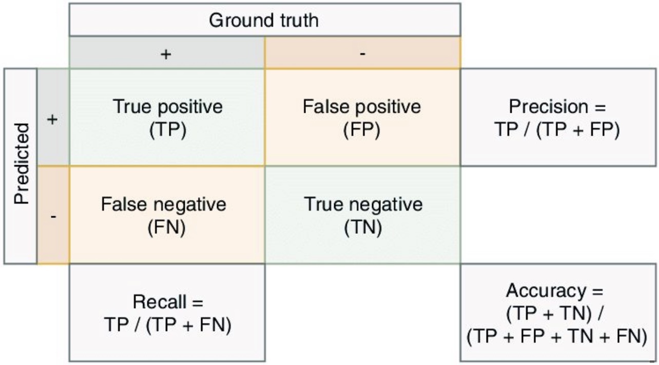
Mathematically, precision and recall are defined as,
\[\operatorname {Precision}=\frac{TP}{TP + FP} \\\] \[\operatorname{Recall}=\frac{TP}{TP + FN} \\\]- where,
- \(TP\) is the True Positive Rate, i.e., the number of instances which are relevant and which the model correctly identified as relevant.
- \(FP\) is the False Positive Rate, i.e., the number of instances which are not relevant but which the model incorrectly identified as relevant.
- \(FN\) is the false negative rate, i.e., the number of instances which are relevant and which the model incorrectly identified as not relevant.
- where,
-
In the content of the robot sifting good apples from the rotten ones,
\[\operatorname {Precision}=\frac{\text { # of picked good apples }}{\text { # of picked apples }}\] \[\operatorname{Recall}=\frac{\text { # of picked good apples }}{\text { # of good apples }}\] -
In the context of information retrieval,
\[\operatorname {Precision}=\frac{\text { retrieved relevant documents }}{\text { all retrieved documents }}\] \[\operatorname{Recall}=\frac{\text { retrieved relevant documents }}{\text { all relevant documents }}\]
Precision/Recall Tradeoff
- Depending on the problem at hand, you either care about high precision or high recall.
- Examples of high precision:
- For a model that detects shop lifters, the focus should be on developing a high precision model by reducing false positives (note that precision is given by \(\frac{TP}{TP+FP}\) and since \(FP\) features in the denominator, reducing \(FP\) leads to high precision). This implies that if we tag someone as a shop lifter, we’d like to make sure we do so with high confidence.
- Examples of high recall:
- In an adult content detection problem, the focus should be on developing a high recall model by reducing false negatives (note that recall is given by \(\frac{TP}{TP+FN}\) and since \(FN\) features in the denominator, reducing \(FN\) leads to high recall). This implies that if the model classified a video as good for kids (i.e., not having adult content), it should be marked so with high confidence.
- In a disease detection scenario, the focus should be on developing a high recall model by reducing false negatives. This implies that if the model classified a patient as not having the disease, it should be done do with high confidence else it can prove fatal.
- In an autonomous car driving scenario, the focus should be on developing a high recall model by reducing false negatives. This implies that if the model determined that there was no obstacle in the car’s surrounding radius, it should be done do with high confidence else fatalities can occur.
- Often, there is an inverse relationship between precision and recall, where it is possible to increase one at the cost of reducing the other. This is called the precision/recall tradeoff. However, in some scenarios, it is important to strike the right balance between both:
- As an example (from the Wikipedia article on Precision and Recall), brain surgery provides an illustrative example of the tradeoff. Consider a brain surgeon removing a cancerous tumor from a patient’s brain. The surgeon needs to remove all of the tumour cells since any remaining cancer cells will regenerate the tumor. Conversely, the surgeon must not remove healthy brain cells since that would leave the patient with impaired brain function. The surgeon may be more liberal in the area of the brain he removes to ensure he has extracted all the cancer cells. This decision increases recall but reduces precision. On the other hand, the surgeon may be more conservative in the brain he removes to ensure he extracts only cancer cells. This decision increases precision but reduces recall. That is to say, greater recall increases the chances of removing healthy cells (negative outcome) and increases the chances of removing all cancer cells (positive outcome). Greater precision decreases the chances of removing healthy cells (positive outcome) but also decreases the chances of removing all cancer cells (negative outcome).
Receiver Operating Characteristic (ROC) Curve
- Suppose we have the probability prediction for each class in a multiclass classification problem, and as the next step, we need to calibrate the threshold on how to interpret the probabilities. Do we predict a positive outcome if the probability prediction is greater than 0.5 or 0.3? The Receiver Operating Characteristic (ROC) curve ROC helps answer this question.
- Adjusting threshold values like this enables us to improve either precision or recall at the expense of the other. For this reason, it is useful to have a clear view of how the False Positive Rate and True Positive Rate vary together.
- The ROC curve shows the variation of the error rates for all values of the manually-defined threshold. The curve is a plot of the False Positive Rate (also called the False Acceptance Rate) on the X-axis versus the True Positive Rate on the Y-axis for a number of different candidate threshold values between 0.0 and 1.0. A data analyst may plot the ROC curve and choose a threshold that gives a desirable balance between the false positives and false negatives.
- False Positive Rate (also called the False Acceptance Rate) on the X-axis: the False Positive Rate is also referred to as the inverted specificity where specificity is the total number of true negatives divided by the sum of the number of true negatives and false positives.
- True Positive Rate on the Y-axis: the True Positive Rate is calculated as the number of true positives divided by the sum of the number of true positives and the number of false negatives. It describes how good the model is at predicting the positive class when the actual outcome is positive.
- Note that both the False Positive Rate and the True Positive Rate are calculated for different probability thresholds.
- As another example, if a search engine assigns a score to all candidate documents that it has retrieved, we can set the search engine to display all documents with a score greater than 10, or 11, or 12. The freedom to set this threshold value generates a smooth curve as below. The figure below shows a ROC curve for a binary classifier with AUC = 0.93. The orange line shows the model’s false positive and false negative rates, and the dotted blue line is the baseline of a random classifier with zero predictive power, achieving AUC = 0.5.

- Note that another way to obtain FPR and TPR is through TNR and FNR respectively, as follows:
- Note that the equal error rate (EER) in ROC curves is obtained as follows:
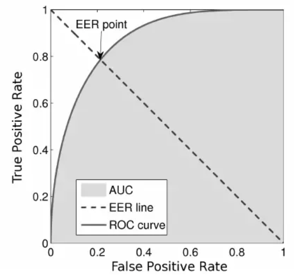
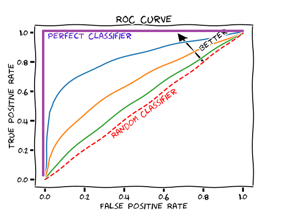
- Also, the \(y = x\) line in the ROC curve signifies the performance of a random classifier (so we need our curve to nudge towards the top-left to yield better AUC and thus better performance than a random classifier):
Detection error tradeoff (DET) curve
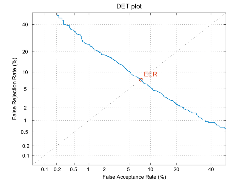
- A detection error tradeoff (DET) curve is a graphical plot of error rates for binary classification systems, plotting the false rejection rate (FRR) vs. false acceptance rate (FAR) for different probability thresholds.
- The X- and Y-axes are scaled non-linearly by their standard normal deviates (or just by logarithmic transformation), yielding tradeoff curves that are more linear than ROC curves, and use most of the image area to highlight the differences of importance in the critical operating region.
Comparing ROC and DET curves
-
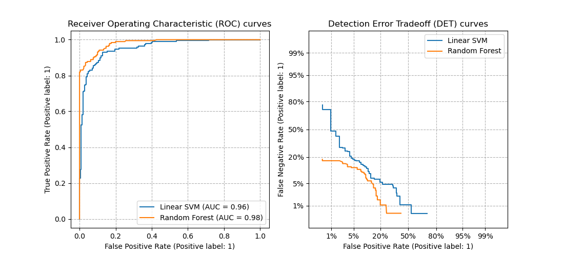
Let’s compare receiver operating characteristic (ROC) and detection error tradeoff (DET) curves for different classification algorithms for the same classification task.
-
DET curves are commonly plotted in normal deviate scale. To achieve this the DET display transforms the error rates as returned by sklearn’s det_curve and the axis scale using
scipy.stats.norm. -
The point of this example is to demonstrate two properties of DET curves, namely:
-
It might be easier to visually assess the overall performance of different classification algorithms using DET curves over ROC curves. Due to the linear scale used for plotting ROC curves, different classifiers usually only differ in the top left corner of the graph and appear similar for a large part of the plot. On the other hand, because DET curves represent straight lines in normal deviate scale. As such, they tend to be distinguishable as a whole and the area of interest spans a large part of the plot.
-
DET curves give the user direct feedback of the detection error tradeoff to aid in operating point analysis. The user can deduct directly from the DET-curve plot at which rate false-negative error rate will improve when willing to accept an increase in false-positive error rate (or vice-versa).
-
-
The plots in this example compare the ROC curve on the left with the corresponding DET curve on the right. There is no particular reason why these classifiers have been chosen for the example plot over other classifiers available in scikit-learn.
- Note that the equal error rate (EER) in DET curves is the intersection of the \(y = x\) line with the DET curve:
- To generate DET curves using scikit-learn:
import numpy as np
from sklearn.metrics import det_curve

y_true = np.array([0, 0, 1, 1])
y_scores = np.array([0.1, 0.4, 0.35, 0.8])

fpr, fnr, thresholds = det_curve(y_true, y_scores)
# fpr: 			array([0.5, 0.5, 0. ])
# fnr: 			array([0. , 0.5, 0.5])
# thresholds: 	array([0.35, 0.4 , 0.8 ])
-
Note the formulae to obtain FAR (FPR) and FRR (FNR):
\[FAR = FPR = \frac{FP}{\text{number of negatives}} = \frac{FP}{FP + TN} \\ FRR = FNR = \frac{FP}{\text{number of positives}} = \frac{FN}{FN + TP}\]- where, FP: False positive; FN: False Negative; TN: True Negative; TP: True Positive
-
Another way to obtain FAR and FRR is through TNR and TPR respectively, as follows:
Area under the ROC Curve (AUC)
- The area under the ROC curve (AUROC) is a good metric for measuring the classifier’s performance. This value is normally between 0.5 (for a bad classifier) and 1.0 (a perfect classifier). The better the classifier, the higher the AUC and the closer the ROC curve will be to the top left corner.
Precision-Recall Curve
- We saw earlier that when a dataset has imbalanced classes, precision and recall are better metrics than accuracy. Similarly, for imbalanced classes, a Precision-Recall curve is more suitable than a ROC curve.
- A Precision-Recall curve is a plot of the Precision (y-axis) and the Recall (x-axis) for different thresholds, much like the ROC curve. Note that in computing precision and recall there is never a use of the true negatives, these measures only consider correct predictions.
Area Under the PR Curve (AUC)
- Similar to the AUROC, the PR AUC summarizes the curve with a range of threshold values as a single score.
- The score can then be used as a point of comparison between different models on a binary classification problem where a score of 1.0 represents a model with perfect skill.
Key takeaways: Precision, Recall and ROC/PR Curves
- ROC Curve: summaries the trade-off between the True Positive Rate and False Positive Rate for a predictive model using different probability thresholds.
- Precision-Recall Curve: summaries the trade-off between the True Positive Rate and the positive predictive value for a predictive model using different probability thresholds.
- In the same way it is better to rely on precision and recall rather than accuracy in an imbalanced dataset scenario (since it can offer you an incorrect picture of the classifier’s performance), a Precision-Recall curve is better to calibrate the probability threshold compared to the ROC curve. In other words, ROC curves are appropriate when the observations are balanced between each class, whereas precision-recall curves are appropriate for imbalanced datasets. In both cases, the area under the curve (AUC) can be used as a summary of the model performance.
| Metric | Formula | Description |
|---|---|---|
| Accuracy | $$\frac{TP+TN}{TP+TN + FP+FN}$$ | Overall performance of model |
| Precision | $$\frac{TP}{TP + FP}$$ | How accurate the positive predictions are |
| Recall/Sensitivity | $$\frac{TP}{TP + FN}$$ | Coverage of actual positive sample |
| Specificity | $$\frac{TN}{TN + FP}$$ | Coverage of actual negative sample |
| F1-score | $$2 \times\frac{\textrm{Precision} \times \textrm{Recall}}{\textrm{Precision} + \textrm{Recall}}$$ | Harmonic mean of Precision and Recall |
Speech Recognition
Speech-to-Speech Machine Translation
- BLEU (BiLingual Evaluation Understudy)
- METEOR (Metric for Evaluation of Translation with Explicit ORdering)
Manual evaluation by humans for fluency, grammar, comparative ranking, etc.
🤗 Open ASR Leaderboard
- The Hugging Face ASR Leaderboard ranks and evaluates speech recognition models on the Hugging Face Hub.
- They report the Average WER and RTF – lower the better. Models are ranked based on their Average WER, from lowest to highest.

Popular Models
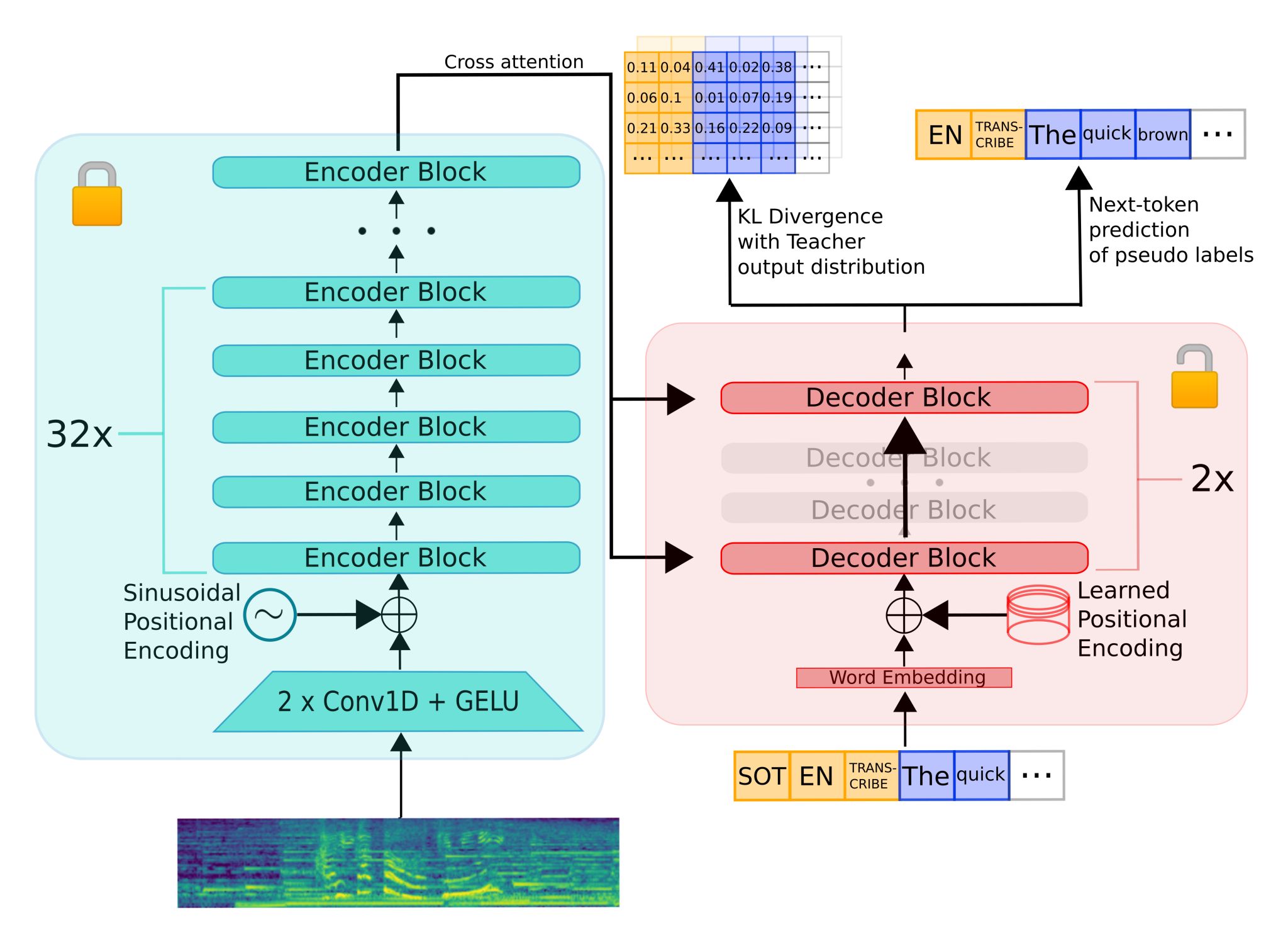
Distil-Whisper
- HuggingFace’s distil-whisper: Distilled OpenAI’s Whisper on 20,000 hours of open-sourced audio data.
- Distil-Whisper is significantly smaller and faster (5.8 times faster, 51% fewer parameters) than the original Whisper model, maintaining similar performance (within 1% WER) on out-of-distribution test data in a zero-shot setting.
- The authors use a large-scale pseudo-labelling approach to assemble an open-source dataset for training, selecting high-quality pseudo-labels based on a word error rate (WER) heuristic.
- The motivation was the fact that OpenAI’s Whisper yields astonishing accuracy for most audio, but it’s too slow and expensive for most production use cases. In addition, it has a tendency to hallucinate.
- Encoding takes \(O(1)\) passes while decoding takes \(O(N)\). This implies that reducing decoder layers is \(N\) time more effective. They kept the whole encoder, but utilized only two decoder layers.
- The encoder is frozen during distillation to ensure Whisper’s robustness to noise is kept.
- The model demonstrates improved robustness against hallucination errors in long-form audio, and its design allows it to be paired with Whisper for speculative decoding, doubling the inference speed while maintaining output accuracy.
- The paper highlights the utility of large-scale pseudo-labelling in speech recognition and the effectiveness of the WER threshold filter in distillation. The training and inference code, along with the models, are made publicly available by the authors.
- To make sure Distil-Whisper does not inherit hallucinations, they filtered out all data samples below a certain WER threshold. By doing so, we were able to reduce hallucinations and actually beat the teacher on long-form audio evaluation.
- The checkpoints are here and also directly available in 🤗 Transformers. All with MIT License.
Parakeet
- Parakeet is jointly developed by NVIDIA NeMo and Suno.ai teams. It is up to 10x faster and 30% more accurate than Whisper models!
- Parakeet is an XXL version of FastConformer Transducer (around 1.1B parameters) model that only supports the English language. The model was trained on 64K hours of English speech collected and prepared by NVIDIA NeMo and Suno teams using NeMo toolkit for over several hundred epochs.
Canary
- Canary-1B, with 1 billion parameters, is trained to excel in automatic speech-to-text recognition (ASR) and translation tasks, supporting English, German, French, and Spanish.
- Model Highlights:
- Language Support: Fluent in 4 languages for ASR and capable of translating between English and German/French/Spanish, including punctuation and capitalization control.
- Architecture: An innovative encoder-decoder setup combining a FastConformer encoder with a Transformer Decoder, ensuring efficient and accurate text generation.
- Ease of Use: Leveraging concatenated SentencePiece tokenizers for scalability and simplicity in language expansion.
- Getting Started with NeMo:
- To harness the power of Canary-1B, NVIDIA recommends installing the NeMo toolkit post-Cython and the latest PyTorch version. This toolkit not only facilitates model training and fine-tuning but also simplifies the inference process for developers and researchers.
- Usage and Performance:
- Canary-1B shines in both ASR and AST (automatic speech-to-text translation), providing exceptional accuracy and versatility. Whether you’re translating speeches or transcribing multi-lingual audio files, Canary-1B delivers with precision. It’s trained on a diverse dataset totaling 85k hours of speech, ensuring robust performance across its supported languages.
- Demo; Model
Suggested Videos
- Deep Learning in Speech Recognition by Alex Acero, Apple Inc.
- End-to-End Models for Speech Processing at Stanford by Navdeep Jaitly, NVIDIA
- Speech Recognition (ASR) by Andrew Senior, Google
- Text to Speech (TTS) by Andrew Senior, Google
- Automatic Speech Recognition: An Overview by Preethi Jyothi, IIT Bombay
- Machine Learning and Causal Inference by Susan Athey, Stanford
References
- Speech Technology - Kishore Prahallad
- Speech and Language Processing by Jurafsky and Martin, 2nd Edition, 2008
- Interspeech 2017 Series Acoustic Model for Speech Recognition Technology
- What’s the difference between a phoneme, a phone, and an allophone?
- Speaker Verification and Identification
- Understanding automatic speech recognition (ASR)
- Gap between DNN and HMM
Acknowledgements
- Thanks to Bharani Kempaiah for helping proof-read this article and offering suggestions for improvement.
Citation
If you found our work useful, please cite it as:
@article{Chadha2020DistilledSpeechProcessing,
  title   = {Speech Processing},
  author  = {Chadha, Aman and Kempaiah, Bharani},
  journal = {Distilled AI},
  year    = {2020},
  note    = {\url{https://aman.ai}}
}