Primers • Residual/Skip Connections
- Overview
- The vanishing gradient problem
- Prelude: Backpropagation
- Backpropagation and partial derivatives
- Skip connections for the win
- ResNet: skip connections via addition
- DenseNet: skip connections via concatenation
- Short and Long skip connections in Deep Learning
- Case Study for long skip connections: U-Nets
- Conclusion
- Related Papers
- Evolution of Skip Connections
- Overview
- Attention Residuals
- Manifold-Constrained Hyper-Connections
- From Hyper-Connections to constrained residual topology
- Failure mode: loss of identity mapping
- Core idea: manifold-constrained residual mappings
- Why doubly stochastic constraints restore stability
- Architectural comparison
- Parameterization and projection
- Dynamic residual mappings
- Systems and efficiency considerations
- Stability and scaling behavior
- Interpretation
- Unifying perspective
- Comparative design guidance
- References
- Foundational residual connections and identity mapping
- Skip connections in segmentation and biomedical vision
- Transformer architectures and residual design evolution
- Attention Residuals and depth-wise aggregation
- Hyper-Connections and residual stream generalization
- Manifold-Constrained Hyper-Connections and stability
- Optimization, scaling, and efficiency
- Books and blogs
- Citation
Overview
-
In order to understand the plethora of design choices involved in building deep neural nets (such as skip connections) that you see in so many works, it is critical to understand a little bit of the mechanisms of backpropagation.
-
If you were trying to train a neural network back in 2014, you would definitely observe the so-called vanishing gradient problem. In simple terms: you are behind the screen checking the training process of your network and all you see is that the training loss stopped decreasing but your performance metric is still far away from the desired value. You check all your code lines to see if something was wrong all night and you find no clue. Not the best experience in the world, believe me! Wonder why? Because the gradients that facilitate learning weren’t propagating through all the way to the initial layers of the network! Hence leading to “vanishing gradients”!
The vanishing gradient problem
-
So, let’s remind ourselves the update rule of gradient descent without momentum, given \(L\) to be the loss function and \(\lambda\) the learning rate:
\[w_{new} = w_{current} - \alpha \cdot \frac{\partial L}{\partial w_{current}}\] -
What is basically happening is that you try to update the parameters by changing them with a small amount \(\alpha \cdot \frac{\partial L}{\partial w_{current}}\) that was calculated based on the gradient, for instance, let’s suppose that for an early layer the average gradient \(\frac{\partial L}{\partial w_{current}} = 1e-15\). Given a learning rate \(\alpha\) of \(1e-4\), you basically change the layer parameters by the product of the referenced quantities \((\alpha \cdot \frac{\partial L}{\partial w_{current}})\), which is \(1e-19\), and as such, implies little to no change to the weights. As a result, you aren’t actually able to train your network. This is the vanishing gradient problem.
Prelude: Backpropagation
-
One can easily grasp the vanishing gradient problem from the backpropagation algorithm. We will briefly inspect the backpropagation algorithm from the prism of the chain rule, starting from basic calculus to gain an insight on skip connections. In short, backpropagation is the “optimization-magic” behind deep learning architectures. Given that a deep network consists of a finite number of parameters that we want to learn, our goal is to iteratively optimize these parameters using the gradient of the loss function \(L\) with respect to the network’s parameters.
-
As you have seen, each architecture has some input (say an image) and produces an output (prediction). The loss function is heavily based on the task we want to solve. For now, what you need to know is the loss function is a quantitative measure of the distance between two tensors, that can represent an image label, a bounding box in an image, a translated text in another language etc. You usually need some kind of supervision to compare the network’s prediction with the desired outcome (ground truth).
-
So, the beautiful idea of backpropagation is to gradually minimize this loss by updating the parameters of the network. But how can you propagate the scalar measured loss inside the network? That’s exactly where backpropagation comes into play.
Backpropagation and partial derivatives
- In simple terms, backpropagation is about understanding how changing the weights (parameters) in a network impacts the loss function by computing the partial derivatives. For the latter, we use the simple idea of the chain rule, to minimize the distance in the desired predictions. In other words, backpropagation is all about calculating the gradient of the loss function while considering the different weights within that neural network, which is nothing more than calculating the partial derivatives of the loss function with respect to model parameters. By repeating this step many times, we will continually minimize the loss function until it stops reducing, or some other predefined termination criteria are met.
Chain rule
- The chain rule basically describes the gradient (rate of change) of a function with respect to some input variable. Let the function be the loss function \(z\) of a neural network, while \(x\) and \(y\) be parameters of the neural network, which are in turn functions of a previous layer parameter \(t\). Further, let \(f, g, h\) be different layers on the network that perform a non-linear operation on the input vector. As such,
- Using the chain rule of multi-variate calculus to express the gradient of \(z\) with respect to the input \(t\):
-
Interestingly, the famous algorithm does exactly the same operation but in the opposite way: it starts from the output \(z\) and calculates the partial derivatives of each parameter, expressing it only based on the gradients of the later layers.
-
It’s really worth noticing that all these values are often less than 1, independent of the sign. In order to propagate the gradient to the earlier layer’s, backpropagation uses multiplication of the partial derivatives (as in the chain rule). For every layer that we go backwards in the network, the gradient of the network gets smaller and smaller owing to multiplication of the upstream gradient with absolute value less than 1 to compute the downstream gradient at every layer (since \(\text{downstream gradient = local gradient }\times\text{ upstream gradient}\)).
Skip connections for the win
-
Skip connections are standard in many convolutional architectures. By using a skip connection, we provide an alternative path for the gradient (with backpropagation). It is experimentally validated that this additional paths are often beneficial for model convergence during training. As the name suggests, skip connections in deep architectures, skip some layer in the neural network and feed the output of one layer as the input to the next layers (instead of only the next one).
-
As previously explained, using the chain rule, we must keep multiplying terms with the error gradient as we go backwards. However, in the long chain of multiplication, if we multiply many things together that are less than one, then the resulting gradient will be very small. Thus, the gradient becomes very small as we approach the earlier layers in a deep architecture. In some cases, the gradient becomes zero, meaning that we do not update the early layers at all.
-
In general, there are two fundamental ways that one could use skip connections through different non-sequential layers:
- Addition as in residual architectures,
- Concatenation as in densely connected architectures.
-
Let’s first do a walk-through of skip connections via addition, which are commonly referred as residual skip connections.
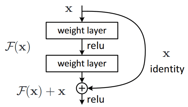
ResNet: skip connections via addition
- The core idea is to backpropagate through the identity function, by just using a vector addition. Then the gradient would simply be multiplied by one and its value will be maintained in the earlier layers. This is the main idea behind Residual Networks (ResNets): they stack these skip residual blocks together, as shown in the figure below (image taken from the ResNet paper). We use an identity function to preserve the gradient.
-
Mathematically, we can represent the residual block, and calculate its partial derivative (gradient), given the loss function like this:
\[\frac{\partial L}{\partial x } = \frac{\partial L}{\partial H} \frac{\partial H}{\partial x} = \frac{\partial L}{\partial H} \left( \frac{\partial F}{\partial x} + 1 \right) = \frac{\partial L}{\partial H} \frac{\partial F}{\partial x} + \frac{\partial L}{\partial H}\]- where \(H\) is the output of the network snippet above and is given by \(F(x) + x\)
-
Apart from the vanishing gradients, there is another reason that we commonly use them. For a plethora of tasks (such as semantic segmentation, optical flow estimation, etc.) information captured in the initial layers could be utilized by the later layers for learning. It has been observed that in earlier layers the learned features correspond to low-level semantic information that is extracted from the input. Without skip connections, that information would have turned too abstract.
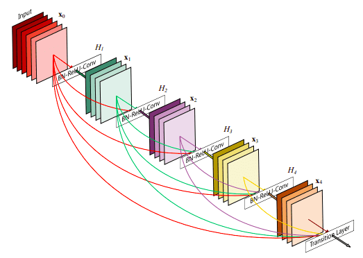
DenseNet: skip connections via concatenation
- As stated, for many dense prediction problems, there is low-level information shared between the input and output, and it would be desirable to pass this information directly across the net. The alternative way that you can achieve skip connections is by concatenation of previous feature maps. The most famous deep learning architecture is DenseNet. Below you can see an example of feature reusability by concatenation with five convolutional layers (image taken from DenseNet):
-
This architecture heavily uses feature concatenation so as to ensure maximum information flow between layers in the network. This is achieved by connecting via concatenation all layers directly with each other, as opposed to ResNets. Practically, what you basically do is to concatenate the feature channel dimension. This leads to:
-
An enormous amount of feature channels on the last layers of the network,
-
More compact models and,
-
Extreme feature re-usability.
-
Short and Long skip connections in Deep Learning
-
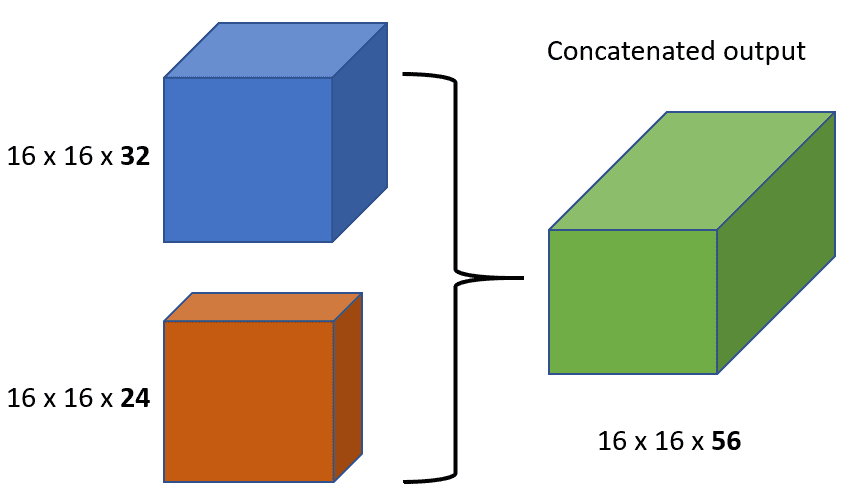
In more practical terms, you have to be careful when introducing additive skip connections in your deep learning model. The dimensionality has to be the same in addition and also in concatenation apart from the chosen channel dimension. That is the reason why you see that additive skip connections are used in two kinds of setups:
-
Short skip connections.
-
Long skip connections.
-
-
Short skip connections are used along with consecutive convolutional layers that do not change the input dimension (see ResNet), while long skip connections usually exist in encoder-decoder architectures. It is known that the global information (shape of the image and other statistics) resolves what, while local information resolves where (small details in an image patch).
-
Long skip connections often exist in architectures that are symmetrical, where the spatial dimension is gradually reduced in the encoder part and is gradually increased in the decoder part as illustrated below. In the decoder part, one can increase the dimensionality of a feature map via transpose convolutional (ConvT) layers. The transposed convolution operation forms the same connectivity as the normal convolution but in the backward direction.
Case Study for long skip connections: U-Nets
-
Mathematically, if we express convolution as a matrix multiplication, then transpose convolution is the reverse order multiplication (\(B \times A\) instead of \(A \times B\)). The aforementioned architecture of the encoder-decoder scheme along with long skip connections is often referred as U-shape (U-net). Long skip connections are utilized for tasks that the prediction has the same spatial dimension as the input such as image segmentation, optical flow estimation, video prediction, etc.
-
Long skip connections can be formed in a symmetrical manner, as shown in the diagram below:
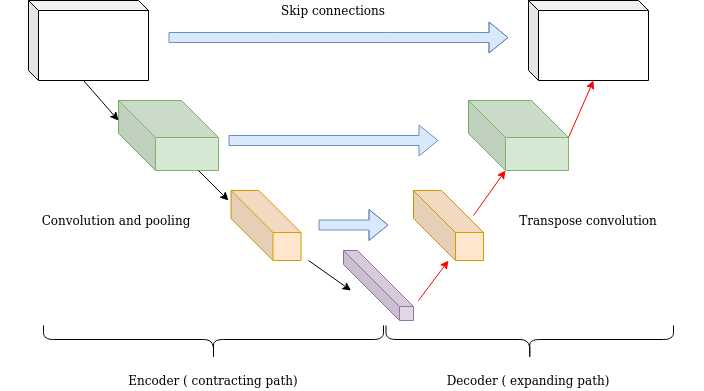
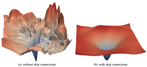
- By introducing skip connections in the encoder-decoded architecture, fine-grained details can be recovered in the prediction. Even though there is no theoretical justification, symmetrical long skip connections work incredibly effectively in dense prediction tasks (medical image segmentation).
Conclusion
-
To sum up, the motivation behind skip connections is that they enable an uninterrupted gradient flow during training, which helps tackle the vanishing gradient problem. Concatenative skip connections enable an alternative way to ensure feature reusability of the same dimensionality from the earlier layers and are widely used in symmetrical architectures.
-
On the other hand, long skip connections are used to pass features from the encoder path to the decoder path in order to recover spatial information lost during downsampling. Short skip connections appear to stabilize gradient updates in deep architectures. Overall, skip connections thus enable feature reusability and stabilize training and convergence.
-
In “Visualizing the Loss Landscape of Neural Nets” by Li et al. (2017), it has been experimentally validated that the loss landscape changes significantly when introducing skip connections, as illustrated below:
Related Papers
Deep Residual Learning for Image Recognition
- ResNet paper by He et al. from Facebook AI in CVPR 2016. Most cited in several AI fields.
- The issue of vanishing gradients when training a deep neural network was addressed with two tricks:
- Batch normalization and,
- Short skip connections
- Instead of \(H(x) = F(x)\), the skip connection leads to \(H(x) = F(x) + x\), which implies that the model is learning the difference (i.e., residual), \(F(x) = H(x) - x\).
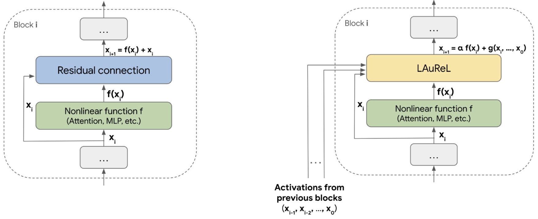
LAUREL: Learned Augmented Residual Layer
-
This paper by Gaurav Menghani, Ravi Kumar, and Sanjiv Kumar from Google Research introduces LAUREL (Learned Augmented Residual Layer), a generalization of the canonical residual connection used in deep learning architectures. LAUREL aims to improve model quality while keeping parameter, latency, and memory overhead minimal, making it suitable as a drop-in replacement in both vision and language models.
-
Core Concept:
- LAUREL extends the standard residual formulation: \(x_{i+1} = f(x_i) + x_i\) to a more expressive form: \(x_{i+1} = \alpha f(x_i) + g(x_i, x_{i-1}, ..., x_0)\) where $\alpha$ is a learnable scalar and $g(\cdot)$ is a learnable linear function over the current and previous layer outputs.
- The goal is to enhance the residual stream to support richer interactions and improved information propagation across layers.
-
Variants:
-
LAUREL-RW (Residual Weights): Introduces learnable weights $\alpha$ and $\beta$ for $f(x_i)$ and $x_i$ respectively: \(x_{i+1} = \alpha f(x_i) + \beta x_i\) Adds only two parameters per layer. Uses sigmoid or softmax to normalize $\alpha$, $\beta$.
-
LAUREL-LR (Low-Rank): Adds a low-rank linear transformation \(W = AB + I\) on \(x_i\): \(x_{i+1} = f(x_i) + B A x_i + x_i\) Reduces parameter growth using matrices $A, B \in \mathbb{R}^{D \times r}$ where $r \ll D$, leading to 2rD new parameters per layer.
-
LAUREL-PA (Previous Activations): Incorporates previous $k$ activations: \(x_{i+1} = f(x_i) + \left( \sum_{j=0}^{k-1} \gamma_{i,j} h_i(x_{i-j}) \right) + x_i\) Adds \(2rD + k\) parameters when using low-rank transforms for $h_i$. Supports richer temporal residual interactions.
-
These can be mixed into hybrid variants like LAUREL-RW+LR or LAUREL-RW+LR+PA, allowing flexibility in trade-offs between expressiveness and cost.
-
-
Implementation and Performance:
-
ResNet-50 on ImageNet-1K:
- Baseline: 74.95% top-1 accuracy.
- Adding one ResNet layer: 75.20% (+4.37% params).
- LAUREL-RW: 75.10% (+0.003% params).
- LAUREL-RW+LR (r=16): 75.20% (+1.68% params).
- LAUREL-RW+LR+PA: 75.25% (+2.40% params), outperforming naive scaling with fewer parameters.
-
1B LLM Pretraining (LLM-1):
- Baseline vs LAUREL-RW+LR (r=4): 0.012% param increase, no measurable latency increase.
- Notable improvements across tasks like GSM8K-CoT (+5.39%), BOOLQ (+13.08%), and BookQA (+20.05%).
-
4B LLM Pretraining (LLM-2):
- LAUREL-RW+LR (r=64): ~0.1% param increase, 1-2% latency increase.
- Improvements on MATH (+4.08%), MGSM (+6.07%), BELEBELE (+8.27%), and multimodal tasks like MMMU (+12.75%).
-
The following figure from the paper shows: (Left) A standard residual connection; the model is divided into logical ‘blocks’, and the residual connection combines the output of a non-linear function \(f\) and the input to this function. (Right) An illustration of the LAUREL framework; LAUREL can be used to replace the regular residual connection. Again, \(f\) can be any non-linear function such as attention, MLPs, and groups of multiple non-linear layers.
-
-
Efficiency and Scalability:
-
LAUREL is designed to be footprint-aware:
- LAUREL-RW: ~constant memory and latency.
- LAUREL-LR: \(\Theta(2rD)\) memory, \(O(rD^2)\) latency.
- LAUREL-PA: \(\Theta(kD)\) memory, \(O(kD)\) latency.
-
LAUREL outperforms naive model scaling both in accuracy and parameter efficiency. For instance, it achieved higher ResNet-50 performance using 2.6× fewer parameters than adding an extra layer.
-
Evolution of Skip Connections
Overview
- Deep Residual Learning for Image Recognition by He et al. (2015) made depth trainable by rewriting a layer as:
- Identity Mappings in Deep Residual Networks by He et al. (2016) clarified why this works: the identity path gives forward activations and backward gradients a direct route across depth. But this same simplicity becomes restrictive in modern LLMs. The residual stream does not decide which earlier layer matters, it simply accumulates every layer output with fixed unit weight:
- This creates three pressure points, as delineated below.
Uniform accumulation dilutes layer contributions
- In PreNorm Transformers, residual states can grow with depth, so each new layer must compete against an increasingly large accumulated state. Attention Residuals by Kimi Team et al. (2026) addresses this by replacing fixed residual addition with learned depth-wise attention, allowing each layer to retrieve earlier representations selectively.
A single residual stream limits cross-depth routing
- Standard residuals preserve information, but they do not provide a learned topology for routing information across layers. Multi-stream extensions such as Hyper-Connections by Zhu et al. (2024) widen the residual stream and introduce learnable mappings between streams, making residual connectivity itself a trainable architectural object rather than a fixed addition rule.
Unconstrained residual mixing can destabilize scale
- Once residual mixing becomes learnable, the identity guarantee that made ResNets stable can be lost. mHC: Manifold-Constrained Hyper-Connections by Xie et al. (2025) solves this by constraining residual mixing matrices to a doubly stochastic manifold, preserving identity-like signal conservation while still allowing multi-stream interaction:
- These newer designs keep the core ResNet insight, namely direct signal propagation, but generalize it in two directions: Attention Residuals make residual aggregation selective across depth, while mHC makes residual topology wider and learnable without giving up stability.
Attention Residuals
Overview
-
Standard residual connections implicitly define a recurrence over depth in which all prior layer outputs are aggregated with equal weight. This can be interpreted as a form of linear attention over depth, where the aggregation weights are fixed and uniform. Attention Residuals by Kimi Team et al. (2026) generalizes this mechanism by introducing content-dependent, learned weighting over previous layers, analogous to how self-attention generalizes recurrence over sequence positions.
-
The core idea is to replace fixed accumulation with a softmax-weighted combination over all preceding layer outputs:
\[h_l = \sum_{i=0}^{l-1} \alpha_{i \to l} \cdot v_i\]-
where:
- $v_0 = h_1$ (embedding)
- $v_i = f_i(h_i)$ for $i \geq 1$
- $\alpha_{i \to l}$ are attention weights satisfying $\sum_i \alpha_{i \to l} = 1$
-
-
This transforms residual connections from a fixed additive structure into a learned depth-wise routing mechanism.
-
The following figure (source) shows an overview of attention residuals: (a) standard residuals: standard residual connections with uniform additive accumulation; (b) full attention residuals: each layer selectively aggregates all previous layer outputs via learned attention weights; (c) block attention residuals: layers are grouped into blocks, reducing memory from \(O(Ld)\) to \(O(Nd)\).

Depth-wise attention formulation
-
Attention Residuals introduce a query-key-value formulation across depth:
\[\alpha_{i \to l} = \frac{\exp\left(q_l^\top \cdot \text{RMSNorm}(k_i)\right)}{\sum_{j=0}^{l-1} \exp\left(q_l^\top \cdot \text{RMSNorm}(k_j)\right)}\]-
with:
\[q_l = w_l, \quad k_i = v_i, \quad v_i = \begin{cases} h_1 & i=0 \\ f_i(h_i) & i \geq 1 \end{cases}\]- where $w_l \in \mathbb{R}^d$ is a learned pseudo-query vector per layer.
-
-
Key properties:
- The query is independent of the forward pass, enabling parallel computation across layers.
- RMS normalization prevents magnitude dominance by deeper layers.
- The formulation is equivalent to softmax attention over depth.
-
This design completes the transition from linear recurrence to attention along the depth dimension, analogous to the transition from RNNs to Transformers over sequence length.
Relationship to standard residual connections
-
Standard residual connections can be recovered as a special case:
\[\alpha_{i \to l} = \frac{1}{l}\]- which corresponds to uniform weighting across all prior layers.
-
More generally, residual connections can be interpreted as:
- Linear attention over depth with fixed kernel
- No content-dependent routing
- Implicit bias toward later layers due to accumulation dynamics
-
Attention Residuals remove these constraints, enabling:
- Selective retrieval of earlier features
- Layer-specific aggregation strategies
- Improved utilization of early-layer representations
Full Attention Residuals
-
In the full formulation, each layer attends over all previous layer outputs. The computational and memory complexity is:
- Computation: \(O(L^2 d)\)
- Memory: \(O(L d)\)
-
Despite the quadratic computation, depth is typically much smaller than sequence length, making this tractable in moderate-scale settings.
-
Implementation details:
- All intermediate activations must be retained
- Attention weights can be computed in parallel across layers due to query independence
- No additional parameters beyond one vector $w_l$ per layer and normalization
-
However, in large-scale distributed training, this introduces:
- Increased activation retention cost
- Communication overhead in pipeline parallelism
Block Attention Residuals
-
To address scalability, Block Attention Residuals partition layers into $N$ blocks, each containing $S = L/N$ layers.
-
Within each block:
- Across blocks, attention is applied over block-level representations:
-
This reduces complexity to:
- Memory: \(O(N d)\)
- Computation: \(O(N^2 d)\)
-
The following figure (source) shows PyTorch-style pseudo-code for block attention residuals (i.e., block-level aggregation and attention), where
block_attn_rescomputes softmax attention over block representations using a learned pseudo-query and the forward pass maintains both completed block summaries and an intra-block partial residual state.

-
Key implementation components:
- Intra-block accumulation: standard residual-style summation within a block
- Inter-block attention: softmax attention over block summaries
- Partial block states: allow fine-grained updates within blocks
Two-phase computation strategy
-
To minimize memory access overhead, Attention Residuals employ a two-phase computation:
- Phase 1: Inter-block attention (batched):
- All queries within a block are evaluated together:
- This amortizes memory reads across $S$ layers.
- Phase 2: Intra-block refinement (sequential):
- Each layer refines its representation using partial block states and merges via online softmax:
-
where:
- $o^{(1)}, \ell^{(1)}$ come from inter-block attention
- $o^{(2)}, \ell^{(2)}$ come from intra-block updates
-
This maintains exact equivalence while reducing I/O overhead.
Training and systems considerations
-
Attention Residuals introduce several system-level challenges:
-
Memory and communication:
- Full AttnRes requires storing all layer outputs
- Pipeline parallelism requires transmitting them across stages
-
Block AttnRes reduces this by:
- Compressing layer outputs into block representations
- Reducing communication from $O(Ld)$ to $O(Nd)$
-
Cross-stage caching:
- Intermediate block representations are cached locally across pipeline stages to avoid redundant communication.
-
Initialization:
- Pseudo-queries are initialized to zero:
-
which yields uniform attention at initialization:
\[\alpha_{i \to l} = \frac{1}{l}\]
-
This ensures a smooth transition from standard residual behavior and prevents early training instability.
Empirical effects
-
Attention Residuals by Kimi Team et al. (2026) demonstrates:
- More uniform hidden-state magnitudes across depth
- Improved gradient distribution
- Consistent gains across model scales
-
These effects directly address the limitations of residual accumulation:
- Preventing dominance of late layers
- Enabling retrieval of early representations
- Improving training stability in deep networks
Interpretation
-
Attention Residuals can be viewed as:
- A depth-wise generalization of self-attention
- A replacement for fixed residual accumulation
- A learned routing mechanism across layers
-
Conceptually:
- ResNet: identity + local transformation
- Hyper-Connections: multi-stream residual mixing
- Attention Residuals: global, content-aware aggregation over depth
-
Together, they represent a shift from static connectivity toward adaptive information flow across network depth.
Manifold-Constrained Hyper-Connections
From Hyper-Connections to constrained residual topology
-
Hyper-Connections generalize residual connections by expanding the residual stream into multiple parallel channels and introducing learnable mappings between them. Instead of a single residual pathway, the model maintains an \(n\)-stream representation:
\[x_l \in \mathbb{R}^{n \times C}\]-
and applies three mappings:
- Pre-mapping $H_l^{pre} \in \mathbb{R}^{1 \times n}$ to compress streams into layer input
- Post-mapping $H_l^{post} \in \mathbb{R}^{1 \times n}$ to expand layer output
- Residual mapping $H_l^{res} \in \mathbb{R}^{n \times n}$ to mix streams
-
-
The forward pass becomes:
-
Hyper-Connections by Zhu et al. (2024) shows that widening the residual stream increases representational capacity without increasing per-layer FLOPs.
-
However, this added flexibility removes a critical invariant: identity mapping.
Failure mode: loss of identity mapping
- In standard residual networks, repeated application of identity connections guarantees stable signal propagation:
- In Hyper-Connections, the equivalent propagation becomes:
-
Because $H_l^{res}$ is unconstrained, the composite mapping:
\[\prod_{i} H_i^{res}\]- can amplify or attenuate signals arbitrarily.
-
The following figure (source) shows training instability in Hyper-Connections, comparing the absolute loss gap and gradient norm behavior of HC and mHC in 27B-model training.

-
This leads to:
- exploding or vanishing residual streams
- unstable gradients
- breakdown of the residual learning principle
-
Empirically, signal amplification can reach orders of magnitude beyond stable regimes.
Core idea: manifold-constrained residual mappings
-
Manifold-Constrained Hyper-Connections (mHC) by Xie et al. (2025) restores stability by constraining $H_l^{res}$ to lie on a specific manifold: the set of doubly stochastic matrices.
-
Formally:
\[H_l^{res} \in \mathcal{M}_{res}\]-
where:
\[\mathcal{M}_{res} = \left\{ H \in \mathbb{R}^{n \times n} \mid H \mathbf{1}_n = \mathbf{1}_n,\; \mathbf{1}_n^\top H = \mathbf{1}_n^\top,\; H \ge 0 \right\}\]
-
-
This manifold is known as the Birkhoff polytope.
Why doubly stochastic constraints restore stability
-
This constraint introduces several critical properties, as delineated below.
-
Norm preservation:
- For any $H_l^{res}$:
- This ensures the mapping is non-expansive, preventing signal explosion.
-
Mean preservation:
- Since rows sum to 1:
- is a convex combination of input streams, preserving the average signal.
-
Compositional closure:
- Products of doubly stochastic matrices remain doubly stochastic:
- This ensures stability across arbitrary depth.
-
Geometric interpretation:
- The Birkhoff polytope is the convex hull of permutation matrices:
- Thus, residual mixing becomes a convex combination of permutations, enabling structured but stable feature mixing.
-
Architectural comparison
-
Residual connections: Use fixed identity mapping, preserving a direct path from shallower to deeper layers through simple addition. This makes optimization stable because gradients can flow through the identity branch without depending entirely on learned transformations. The tradeoff is that the residual path itself is not adaptive: every layer receives the same accumulated stream structure.
-
Hyper-Connections: Use unconstrained learned mixing, making the residual pathway learnable by expanding it into multiple streams and mixing them with trainable matrices. This increases expressivity because information can be routed across streams rather than only carried forward through a single identity path. However, because the mixing matrices are unconstrained, repeated composition across depth can amplify or suppress signals unpredictably.
-
mHC: Uses constrained learned mixing with stability guarantees, keeping the multi-stream expressivity of Hyper-Connections while constraining the residual mixing matrix to a doubly stochastic manifold. This preserves identity-like signal conservation because each stream update behaves like a normalized convex combination of streams. The result is a residual topology that can learn richer routing patterns while maintaining stable forward and backward propagation.
Parameterization and projection
- To enforce the manifold constraint, mHC uses a projection step:
-
This projection is implemented using the Sinkhorn-Knopp algorithm:
- Iteratively normalize rows and columns
- Converges to a doubly stochastic matrix
-
Sinkhorn-Knopp by Sinkhorn and Knopp (1967) provides an efficient iterative procedure for this projection.
-
Implementation details:
- Apply normalization in log-space for numerical stability
- Use entropic regularization to ensure smooth convergence
- Maintain differentiability for backpropagation
Dynamic residual mappings
-
As in Hyper-Connections, mappings are input-dependent:
\[H_l^{res} = \alpha_l^{res} \cdot \tanh(\theta_l^{res} \tilde{x}_l^\top) + b_l^{res}\]-
where:
- $\tilde{x}_l = \text{RMSNorm}(x_l)$
- $\theta_l^{res} \in \mathbb{R}^{n \times C}$
- $b_l^{res} \in \mathbb{R}^{n \times n}$
-
-
After computing this unconstrained matrix, projection enforces the manifold constraint.
-
This yields (i) dynamic, input-conditioned mixing and (ii) bounded and stable transformations.
Systems and efficiency considerations
-
While mHC stabilizes training, it introduces system-level overhead due to:
- expanded residual stream (\(nC\) instead of \(C\))
- additional mappings
- projection operations
-
The paper addresses these through several optimizations:
-
Kernel fusion: Combine multiple operations into a single GPU kernel to reduce memory access overhead.
-
Recomputation: Use selective recomputation to reduce activation memory footprint during backpropagation.
-
Pipeline parallelism optimization: Overlap communication with computation using scheduling strategies such as DualPipe.
-
-
These optimizations mitigate the “memory wall” bottleneck described in modern architectures.
Stability and scaling behavior
- The following figure (source) shows propagation instability in Hyper-Connections, including single-layer and composite residual mapping gain magnitudes for forward signals and backward gradients in a 27B model.

-
mHC addresses this by:
- bounding signal amplification
- stabilizing gradient norms
- preserving identity-like behavior across depth
-
Empirical results show:
- improved training stability at large scale
- better scaling with model size
- minimal additional training overhead (~6.7%)
Interpretation
-
Manifold-Constrained Hyper-Connections represent a synthesis of two competing goals:
- expressivity: enable rich, multi-stream residual interactions
-
stability: preserve identity mapping properties essential for deep training
-
Conceptually:
- ResNet ensures stability via identity
- Hyper-Connections increase capacity via topology
-
mHC constrains topology to preserve stability
-
This introduces a new design principle:
- residual connections can be treated as structured transformations on a constrained manifold, rather than simple additive pathways.
Unifying perspective
-
Together with Attention Residuals:
- Attention Residuals solve how to weight information across depth
- mHC solves how to route information across parallel residual streams
-
Both move beyond static residual addition toward (i) learned, structured aggregation, (ii) controlled signal propagation, and (iii) scalable architectural expressivity.
Comparative design guidance
Choosing the right residual generalization
- Use standard residual connections when the primary requirement is stability, simplicity, and minimal overhead:
-
Use Attention Residuals by Kimi Team et al. (2026) when the main bottleneck is uniform depth-wise accumulation, especially in PreNorm LLMs where fixed residual addition can dilute individual layer contributions.
-
Use mHC: Manifold-Constrained Hyper-Connections by Xie et al. (2025) when the goal is to increase residual-stream capacity through multi-stream routing while preserving the identity-like stability that unconstrained Hyper-Connections by Zhu et al. (2024) can weaken.
Comparison of mechanisms
| Mechanism | What changes | Main benefit | Main cost |
|---|---|---|---|
| ResNet-style residuals | Fixed identity addition | Stable gradient flow | No adaptive routing |
| Attention Residuals | Softmax attention over previous layer outputs | Selective depth-wise retrieval | Extra depth-attention state |
| Block Attention Residuals | Attention over block summaries | Scalable depth-wise retrieval | Coarser layer resolution |
| Hyper-Connections | Multi-stream residual topology | Higher residual capacity | Possible instability |
| mHC | Manifold-constrained multi-stream topology | Capacity with stable signal propagation | Projection and I/O overhead |
Complementary roles
- Attention Residuals and mHC solve different parts of the residual-design problem.
Attention Residuals answer: “Which earlier layer outputs should this layer use?” while mHC answers: “How should information move across parallel residual streams?”
- This distinction is important: Attention Residuals operate across depth, while mHC operates across residual-stream width. In principle, these ideas are not mutually exclusive, since one improves depth-wise selection and the other improves stream-wise routing.
Key takeaway
- The evolution from ResNet residuals to Attention Residuals and mHC suggests a broader design principle: residual connections should no longer be treated as passive addition rules. They can be learned communication structures, provided that their parameterization preserves stable signal propagation.
References
Foundational residual connections and identity mapping
- Learning representations by back-propagating errors by Rumelhart et al. (1986)
- Deep Residual Learning for Image Recognition by He et al. (2015)
- Identity Mappings in Deep Residual Networks by He et al. (2016)
- Highway Networks by Srivastava et al. (2015)
- Densely Connected Convolutional Networks by Huang et al. (2017)
- FractalNet: Ultra-Deep Neural Networks without Residuals by Larsson et al. (2016)
Skip connections in segmentation and biomedical vision
- U-Net: Convolutional Networks for Biomedical Image Segmentation by Ronneberger et al. (2015)
- 3D U-Net: Learning Dense Volumetric Segmentation from Sparse Annotation by Çiçek et al. (2016)
- The Importance of Skip Connections in Biomedical Image Segmentation by Drozdzal et al. (2016)
Transformer architectures and residual design evolution
- Attention Is All You Need by Vaswani et al. (2017)
- Language Models are Few-Shot Learners by Brown et al. (2020)
- LLaMA: Open and Efficient Foundation Language Models by Touvron et al. (2023)
- RMSNorm: Root Mean Square Layer Normalization by Zhang and Sennrich (2019)
Attention Residuals and depth-wise aggregation
- Attention Residuals by Kimi Team et al. (2026)
- Kimi Linear Architecture by Moonshot AI et al. (2024)
- A Survey of Attention Mechanisms in Deep Learning by Chaudhari et al. (2019)
Hyper-Connections and residual stream generalization
- Hyper-Connections by Zhu et al. (2024)
- Residual Matrix Transformer by Mak and Flanigan (2025)
- MUDDFormer: Multiway Dynamic Dense Connections by Xiao et al. (2025)
Manifold-Constrained Hyper-Connections and stability
- mHC: Manifold-Constrained Hyper-Connections by Xie et al. (2025)
- Sinkhorn-Knopp Algorithm for Matrix Scaling by Sinkhorn and Knopp (1967)
Optimization, scaling, and efficiency
- Visualizing the Loss Landscape of Neural Nets by Li et al. (2018)
- Efficient Memory Management for Large Language Model Serving with PagedAttention by Kwon et al. (2023)
- FlashAttention: Fast and Memory-Efficient Exact Attention by Dao et al. (2022)
- Chinchilla Scaling Laws by Hoffmann et al. (2022)
Books and blogs
- Neural Networks and Deep Learning by Nielsen (2018)
- The Annotated Transformer
- Residual Connections Explained
- Understanding Deep Residual Networks
Citation
If you found our work useful, please cite it as:
@article{Chadha2020DistilledSkipConnections,
  title   = {Residual/Skip Connections},
  author  = {Chadha, Aman},
  journal = {Distilled AI},
  year    = {2020},
  note    = {\url{https://aman.ai}}
}