Primers • Parameter Efficient Fine-Tuning
- Overview
- Parameter-Efficient Fine-Tuning (PEFT)
- Advantages
- PEFT methods
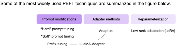
- Prompt Modifications
- Adapters
- Reparameterization
- Low-Rank Adaptation (LoRA)
- Background
- Overview
- Advantages
- Limitations
- Hyperparameters
- How does having a low-rank matrix in LoRA help the fine-tuning process?
- How does low-rank constraint introduced by LoRA inherently act as a form of regularization, especially for the lower layers of the model?
- How does LoRA help avoid catastrophic forgetting?
- How does multiplication of two low-rank matrices in LoRA lead to lower attention layers being impacted less than higher attention layers?
- In LoRA, why is \(A\) initialized using a Gaussian and \(B\) set to 0?
- For a given task, how do we determine whether to fine-tune the attention layers or feed-forward layers?
- Assuming we’re fine-tuning attention weights, which specific attention weight matrices should we apply LoRA to?
- Is there a relationship between setting scaling factor and rank in LoRA?
- How do you determine the optimal rank \(r\) for LoRA?
- How do LoRA hyperparameters interact with each other? Is there a relationship between LoRA hyperparameters?
- Why does a higher rank make it the easier to overfit?
- Does LoRA adapt weights in all layers?
- Quantized Low-Rank Adaptation (QLoRA)
- Quantization-Aware Low-Rank Adaptation (QA-LoRA)
- Refined Low-Rank Adaptation (ReLoRA)
- S-LoRA: Serving Thousands of Concurrent LoRA Adapters
- Weight-Decomposed Low-Rank Adaptation (DoRA)
- Summary of LoRA Techniques
- Low-rank Linear Subspace ReFT (LoReFT)
- Stratified Progressive Adaptation Fine-tuning (SPAFIT)
- BitFit
- NOLA
- Matrix of Rank Adaptation (MoRA)
- Low-Rank Adaptation (LoRA)
- Which PEFT Technique to Choose: A Mental Model
- Comparative Analysis of Popular PEFT Methods
- Practical Tips for Finetuning LLMs Using LoRA
- Related: Surgical fine-tuning
- References
- Citation
Overview
- Fine-tuning of large pre-trained models on downstream tasks is called “transfer learning”.
- While full fine-tuning pre-trained models on downstream tasks is a common, effective approach, it is an inefficient approach to transfer learning.
- The simplest way out for efficient fine-tuning could be to freeze the networks’ lower layers and adapt only the top ones to specific tasks.
- In this article, we’ll explore Parameter Efficient Fine-Tuning (PEFT) methods that enable us to adapt a pre-trained model to downstream tasks more efficiently – in a way that trains lesser parameters and hence saves cost and training time, while also yielding performance similar to full fine-tuning.
Parameter-Efficient Fine-Tuning (PEFT)
- Let’s start off by defining what parameter-efficient fine-tuning is and give some context on it.
- Parameter-efficient fine-tuning is particularly used in the context of large-scale pre-trained models (such as in NLP), to adapt that pre-trained model to a new task without drastically increasing the number of parameters.
- The challenge is this: modern pre-trained models (like BERT, GPT, T5, etc.) contain hundreds of millions, if not billions, of parameters. Fine-tuning all these parameters on a downstream task, especially when the available dataset for that task is small, can easily lead to overfitting. The model may simply memorize the training data instead of learning genuine patterns. Moreover, introducing additional layers or parameters during fine-tuning can drastically increase computational requirements and memory consumption.
- As mentioned earlier, PEFT allows to only fine-tune a small number of model parameters while freezing most of the parameters of the pre-trained LLM. This helps overcome the catastrophic forgetting issue that full fine-tuned Large Language Models (LLMs) face where the LLM forgets the original task it was trained on after being fine-tuned.
- The image below (source) gives a nice overview of PEFT and its benefits.
Advantages
- Parameter-efficient fine-tuning is useful due the following reasons:
- Reduced computational costs (requires fewer GPUs and GPU time).
- Faster training times (finishes training faster).
- Lower hardware requirements (works with cheaper GPUs with less VRAM).
- Better modeling performance (reduces overfitting).
- Less storage (majority of weights can be shared across different tasks).
Practical use-case
- Credits to the below section go to Pranay Pasula.
- PEFT obviates the need for 40 or 80GB A100s to make use of powerful LLMs. In other words, you can fine-tune 10B+ parameter LLMs for your desired task for free or on cheap consumer GPUs.
- Using PEFT methods like LoRA, especially 4-bit quantized base models via QLoRA, you can fine-tune 10B+ parameter LLMs that are 30-40GB in size on 16GB GPUs. If it’s out of your budget to buy a 16GB GPU/TPU, Google Colab occasionally offers a 16GB VRAM Tesla T4 for free. Remember to save your model checkpoints every now and then and reload them as necessary, in the event of a Colab disconnect/kernel crash.
- If you’re fine-tuning on a single task, the base models are already so expressive that you need only a few (~10s-100s) of examples to perform well on this task. With PEFT via LoRA, you need to train only a trivial fraction (in this case, 0.08%), and though the weights are stored as 4-bit, computations are still done at 16-bit.
- Note that while a good amount of VRAM is still needed for the fine-tuning process, using PEFT, with a small enough batch size, and little gradient accumulation, can do the trick while still retaining ‘
FP16’ computation. In some cases, the performance on the fine-tuned task can be comparable to that of a fine-tuned 16-bit model. - Key takeaway: You can fine-tune powerful LLMs to perform well on a desired task using free compute. Use a <10B parameter model, which is still huge, and use quantization, PEFT, checkpointing, and provide a small training set, and you can quickly fine-tune this model for your use case.
PEFT methods
- Below, we will delve into individual PEFT methods and delve deeper into their nuances.
Prompt Modifications
Soft Prompt Tuning
- First introduced in the The Power of Scale for Parameter-Efficient Prompt Tuning; this paper by Lester et al. introduces a simple yet effective method called soft prompt tuning, which prepends a trainable tensor to the model’s input embeddings, essentially creating a soft prompt to condition frozen LLMs to perform specific downstream tasks. Unlike the discrete text prompts, soft prompts are learned through backpropagation and can be fine-tuned to incorporate signals from any number of labeled examples.
- Soft prompt tuning only requires storing a small task-specific prompt for each task, and enables mixed-task inference using the original pre-trained model.
- The authors show that prompt tuning outperforms few-shot learning by a large margin, and becomes more competitive with scale.
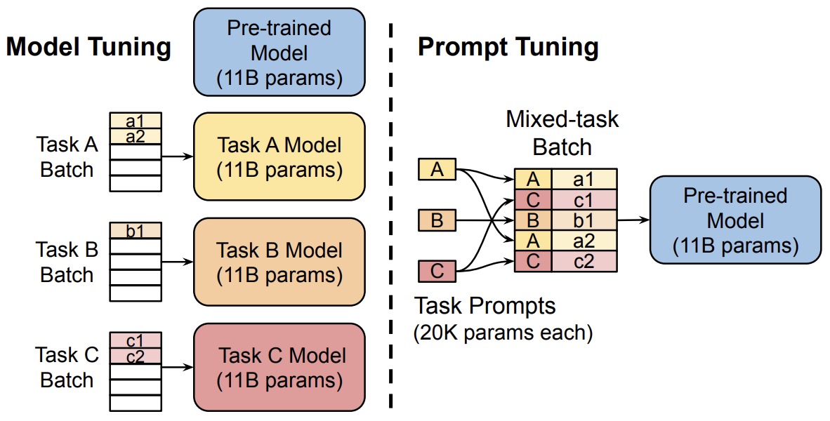
- This is an interesting approach that can help to effectively use a single frozen model for multi-task serving.
- Model tuning requires making a task-specific copy of the entire pre-trained model for each downstream task and inference must be performed in separate batches. Prompt tuning only requires storing a small task-specific prompt for each task, and enables mixed-task inference using the original pretrained model. With a T5 “XXL” model, each copy of the tuned model requires 11 billion parameters. By contrast, our tuned prompts would only require 20,480 parameters per task—a reduction of over five orders of magnitude – assuming a prompt length of 5 tokens.
- Thus, instead of using discrete text prompts, prompt tuning employs soft prompts. Soft prompts are learnable and conditioned through backpropagation, making them adaptable for specific tasks.
- Prompt Tuning offers many benefits such as:
- Memory-Efficiency: Prompt tuning dramatically reduces memory requirements. For instance, while a T5 “XXL” model necessitates 11 billion parameters for each task-specific model, prompt-tuned models need a mere 20,480 parameters (assuming a prompt length of 5 tokens).
- Versatility: Enables the use of a single frozen model for multi-task operations.
- Performance: Outshines few-shot learning and becomes more competitive as the scale grows.
Soft Prompt vs. Prompting
- Soft prompt tuning and prompting a model with extra context are both methods designed to guide a model’s behavior for specific tasks, but they operate in different ways. Here’s how they differ:
- Mechanism:
- Soft Prompt Tuning: This involves introducing trainable parameters (soft prompts) that are concatenated or added to the model’s input embeddings. These soft prompts are learned during the fine-tuning process and are adjusted through backpropagation to condition the model to produce desired outputs for specific tasks.
- Prompting with Extra Context: This method involves feeding the model with handcrafted or predefined text prompts that provide additional context. There’s no explicit fine-tuning; instead, the model leverages its pre-trained knowledge to produce outputs based on the provided context. This method is common in few-shot learning scenarios where the model is given a few examples as prompts and then asked to generalize to a new example.
- Trainability:
- Soft Prompt Tuning: The soft prompts are trainable. They get adjusted during the fine-tuning process to optimize the model’s performance on the target task.
- Prompting with Extra Context: The prompts are static and not trainable. They’re designed (often manually) to give the model the necessary context for the desired task.
- Use Case:
- Soft Prompt Tuning: This method is particularly useful when there’s a need to adapt a pre-trained model to various downstream tasks without adding significant computational overhead. Since the soft prompts are learned and optimized, they can capture nuanced information necessary for the task.
- Prompting with Extra Context: This is often used when fine-tuning isn’t feasible or when working with models in a zero-shot or few-shot setting. It’s a way to leverage the vast knowledge contained in large pre-trained models by just guiding their behavior with carefully crafted prompts.
- In essence, while both methods use prompts to guide the model, soft prompt tuning involves learning and adjusting these prompts, whereas prompting with extra context involves using static, handcrafted prompts to guide the model’s behavior.
Prefix Tuning
- Proposed in Prefix-Tuning: Optimizing Continuous Prompts for Generation, prefix-tuning is a lightweight alternative to fine-tuning for natural language generation tasks, which keeps language model parameters frozen, but optimizes a small continuous task-specific vector (called the prefix).
- Instead of adding a soft prompt to the model input, it prepends trainable parameters to the hidden states of all transformer blocks. During fine-tuning, the LM’s original parameters are kept frozen while the prefix parameters are updated.
- Prefix-tuning draws inspiration from prompting, allowing subsequent tokens to attend to this prefix as if it were “virtual tokens”.
- The figure below from the paper shows that fine-tuning (top) updates all Transformer parameters (the red Transformer box) and requires storing a full model copy for each task. They propose prefix-tuning (bottom), which freezes the Transformer parameters and only optimizes the prefix (the red prefix blocks). Consequently, prefix-tuning only need to store the prefix for each task, making prefix-tuning modular and space-efficient. Note that each vertical block denote transformer activations at one time step.
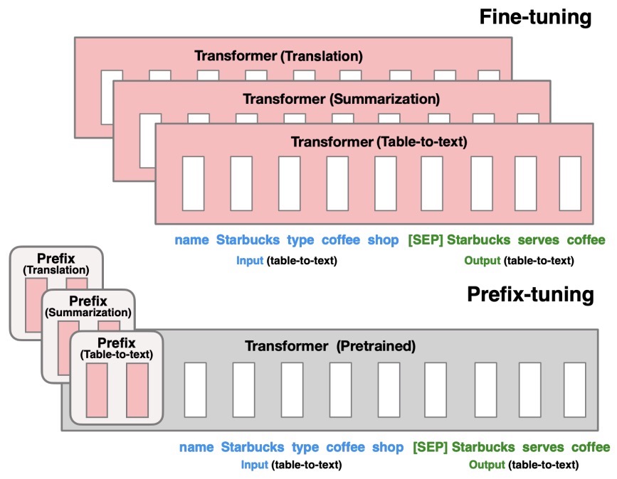
-
They apply prefix-tuning to GPT-2 for table-to-text generation and to BART for summarization. They find that by learning only 0.1% of the parameters, prefix-tuning obtains comparable performance in the full data setting, outperforms fine-tuning in low-data settings, and extrapolates better to examples with topics unseen during training.
-
The image below (source) illustrate how in prefix tuning, trainable tensors are addted to each transformer block instead of only in the input embedding.
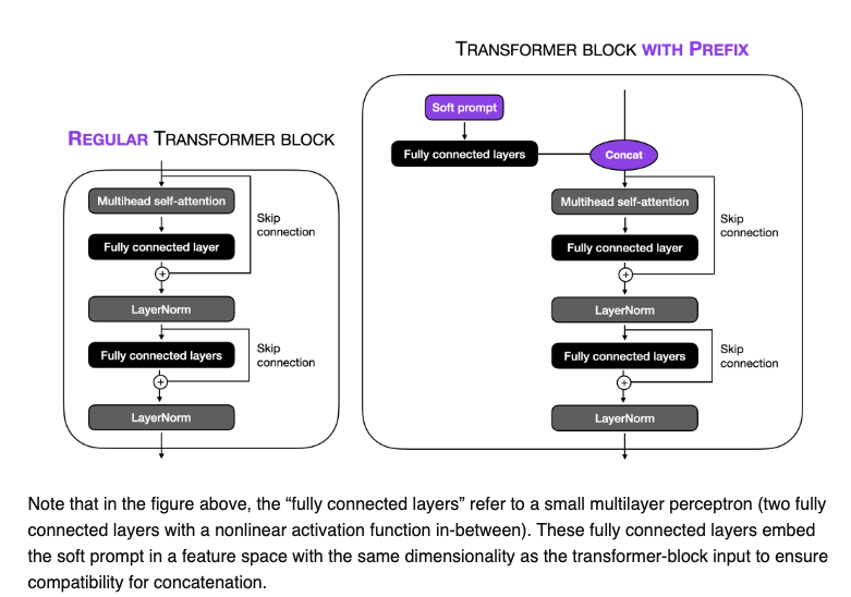
Hard prompt tuning
- Hard prompt tuning directly modifies the input prompt to the model. This can involve a vast multitude of things such as:
- We can add examples of outputs we expect from the prompt
- We can add tags specifically relating to our task at hand
- In essence, it is just the modification of the string input, or prompt, to the model.
Adapters
- Adapter layers, often termed “Adapters”, add minimal additional parameters to the pretrained model. These adapters are inserted between existing layers of the network.
- Adapters is a PEFT technique shown to achieve similar performance as compared to tuning the top layers while requiring as fewer parameters as two orders of magnitude.
- Adapter-based tuning simply inserts new modules called “adapter modules” between the layers of the pre-trained network.
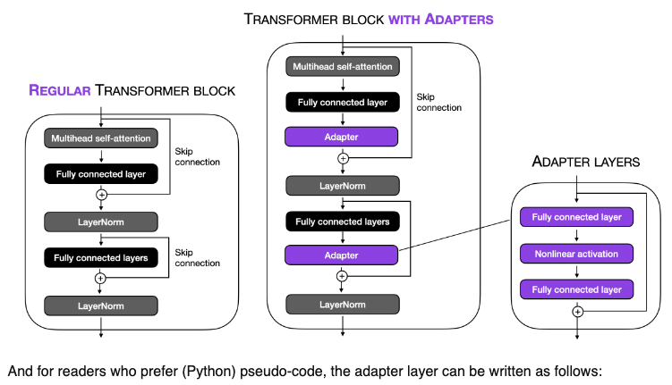
- The image below (source) illustrates this concept for the transformer block:
- During fine-tuning, only the parameters of these adapter layers are updated, while the original model parameters are kept fixed. This results in a model with a small number of additional parameters that are task-specific.
- Keeping the full PT model frozen, these modules are the only optimizable ones while fine-tuning – this means only a very few parameters are introduced per task yielding “compact” models.
- They offer many benefits such as:
- Parameter-Efficiency: By keeping the main model frozen and only updating the adapter layers, a minimal number of parameters are added per task. This results in compact models that are memory-efficient.
- Performance: Despite the small parameter footprint, adapters often achieve performance comparable to conventional fine-tuning.
-
The adapter module consists of two fully connected layers with a bottleneck structure. This structure is inspired by autoencoders, which are designed to encode information into a compressed representation and then decode it back to its original form.
- Here’s how the parameter efficiency is achieved:
-
Bottleneck Structure: The first layer of the adapter reduces the dimensionality of the input (e.g., from 1024 to 24 dimensions). This drastic reduction means that the information from the original 1024 dimensions must be compressed into just 24 dimensions. The second layer then projects these 24 dimensions back to the original 1024 dimensions.
-
Reduction in Parameters: This bottleneck approach significantly reduces the number of parameters. In your example, the total number of parameters introduced by the adapter is 49,152 (from the computation 1024x24 + 24x1024). If we were to use a single fully connected layer to project a 1024-dimensional input to a 1024-dimensional output directly, it would require 1,048,576 parameters (1024x1024).
-
Efficiency Analysis: By using the adapter approach, the number of parameters is substantially lower. Comparing 49,152 parameters to 1,048,576 parameters shows a dramatic reduction, making the adapter much more efficient in terms of parameter usage.
-
Why is this Beneficial?: This efficiency is particularly beneficial when fine-tuning large pre-trained models. Instead of retraining or adapting the entire network (which would be computationally expensive and memory-intensive), adapters allow for targeted adjustments with far fewer additional parameters. This makes the process more manageable and practical, especially when resources are limited.
- The adapter’s bottleneck structure allows it to achieve similar functionality (adapting the model to new tasks or data) as a full-sized layer would, but with a significantly reduced number of parameters. This efficiency makes adapters a popular choice for fine-tuning large pre-trained models in a resource-effective manner.
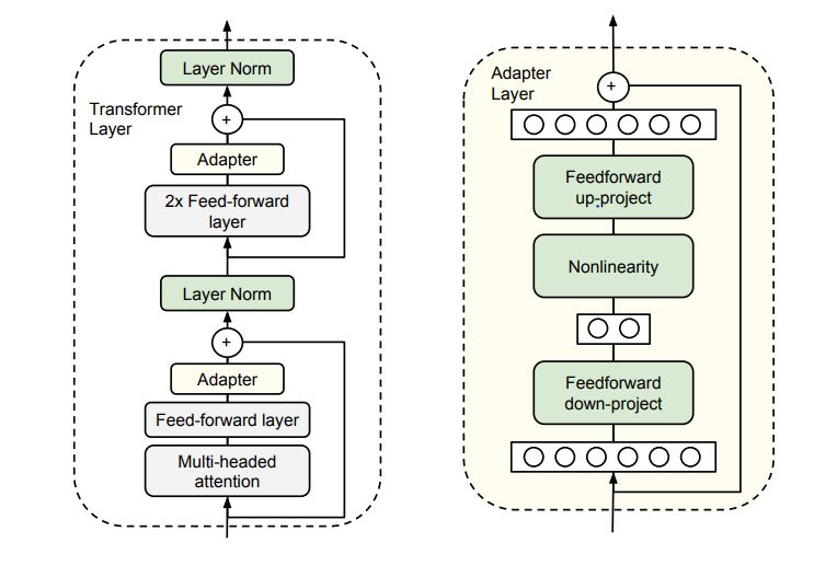
What is an Adapter Module?
- Let’s look at the application of the adapter module in the transformer architecture in three points:
- The adapter module (right) first projects the original \(d\)-dimensional features into a smaller \(m\)-dimensional vector, applies a non-linearity, and then projects it back to \(d\) dimensions.
- As can be seen, the module features a skip-connection - With it in place, when the parameters of the projection layers are initialized to near-zero which eventually leads to near identity initialization of the module. This is required for stable fine-tuning and is intuitive as with it, we essentially do not disturb the learning from pre-training.
- In a transformer block (left), the adapter is applied directly to the outputs of each of the layers (attention and feedforward).
How do you decide the value of \(m\)?
- The size \(m\) in the Adapter module determines the number of optimizable parameters and hence poses a parameter vs performance tradeoff.
- The original paper experimentally investigates that the performance remains fairly stable across varying adapter sizes \(m\) and hence for a given model a fixed size can be used for all downstream tasks.
LLaMA-Adapters
-
This paper introduces an efficient fine-tuning method called LLaMA-Adapter. This method is designed to adapt the LLaMA model into an instruction-following model with high efficiency in terms of resource usage and time. Key aspects of this paper include:
-
Parameter Efficiency: LLaMA-Adapter introduces only 1.2 million learnable parameters on top of the frozen LLaMA 7B model, which is significantly fewer than the full 7 billion parameters of the model. This approach leads to a more efficient fine-tuning process both in terms of computational resources and time, taking less than one hour on 8 A100 GPUs.
-
Learnable Adaption Prompts: The method involves appending a set of learnable adaption prompts to the input instruction tokens in the higher transformer layers of LLaMA. These prompts are designed to adaptively inject new instructions into the frozen LLaMA while preserving its pre-trained knowledge, effectively guiding the subsequent contextual response generation.
-
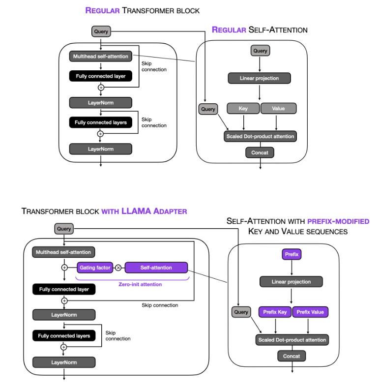
Zero-initialized Attention Mechanism: To avoid disturbances from randomly initialized adaption prompts, which can harm fine-tuning stability and effectiveness, the paper proposes a zero-initialized attention mechanism with a learnable gating factor. This mechanism allows for a stable learning process and progressive incorporation of instructional signals during training. It ensures that the newly acquired instructional signals are effectively integrated into the transformer while retaining the pre-trained knowledge of LLaMA.
-
Generalization and Multi-modal Reasoning: LLaMA-Adapter is not only effective for language tasks but can also be extended to multi-modal instructions, allowing for image-conditioned LLaMA models. This capability enables superior reasoning performance on benchmarks like ScienceQA and COCO Caption. Additionally, the approach has demonstrated strong generalization capacity in traditional vision and language tasks.
-
-
In summary, the LLaMA-Adapter represents a significant advancement in the field of parameter-efficient fine-tuning of large LLMs. Its innovative use of learnable adaption prompts and zero-initialized attention mechanism provides a highly efficient method for adapting pre-trained models to new tasks and domains, including multi-modal applications.
-
The image below (source) illustrates this concept below.
Reparameterization
Low-Rank Adaptation (LoRA)
Background
Rank of a Matrix
- The rank of a matrix is a measure of the number of linearly independent rows or columns in the matrix.
- If a matrix has rank 1, it means all rows or all columns can be represented as multiples of each other, so there’s essentially only one unique “direction” in the data.
- A full-rank matrix has rank equal to the smallest of its dimensions (number of rows or columns), meaning all rows and columns are independent.
-
On a related note, a matrix is said to be rank-deficient if it does not have full rank. The rank deficiency of a matrix is the difference between the lesser of the number of rows and columns, and the rank. For more, refer Wikipedia: Rank.
-
Example:
- Consider the following 3x3 matrix \(A\):
-
Step-by-Step to Determine the Rank:
-
Row Reduction: To find the rank, we can use Gaussian elimination to transform the matrix into its row echelon form, making it easier to see linearly independent rows.
After row-reducing \(A\), we get:
\[A = \begin{bmatrix} 1 & 2 & 3 \\ 0 & -3 & -6 \\ 0 & 0 & 0 \end{bmatrix}\] -
Count Independent Rows: Now we look at the rows with non-zero entries:
- The first row \([1, 2, 3]\) is non-zero.
- The second row \([0, -3, -6]\) is also non-zero and independent of the first row.
- The third row is all zeros, which does not contribute to the rank.
Since there are two non-zero, independent rows in the row echelon form, the rank of \(A\) is 2.
-
-
Explanation:
- The rank of 2 indicates that only two rows or columns in \(A\) contain unique information, and the third row (or column) can be derived from a combination of the other two. Essentially, this matrix can be thought of as existing in a 2-dimensional space rather than a full 3-dimensional space, despite its 3x3 size.
- In summary:
- The rank of matrix \(A\) is 2.
- This rank tells us the matrix’s actual dimensionality in terms of its independent information.
Related: Rank of a Tensor
- While LoRA injects trainable low-rank matrices, it is important to understand rank in the context of tensors as well.
-
The rank of a tensor refers to the number of dimensions in the tensor. This is different from the rank of a matrix, which relates to the number of linearly independent rows or columns. For tensors, rank simply tells us how many dimensions or axes the tensor has.
-
Explanation with Examples:
- Scalar (Rank 0 Tensor):
- A scalar is a single number with no dimensions.
- Example:
5or3.14 - Shape:
()(no dimensions) - Rank: 0
- Vector (Rank 1 Tensor):
- A vector is a one-dimensional array of numbers.
- Example:
[3, 7, 2] - Shape:
(3,)(one dimension with 3 elements) - Rank: 1
- Matrix (Rank 2 Tensor):
- A matrix is a two-dimensional array of numbers, like a table.
- Example: \(\begin{bmatrix} 1 & 2 & 3 \\ 4 & 5 & 6 \end{bmatrix}\)
- Shape:
(2, 3)(two dimensions: 2 rows, 3 columns) - Rank: 2
- 3D Tensor (Rank 3 Tensor):
- A 3D tensor can be thought of as a “stack” of matrices, adding a third dimension.
- Example: \(\begin{bmatrix} \begin{bmatrix} 1 & 2 & 3 \\ 4 & 5 & 6 \end{bmatrix}, \begin{bmatrix} 7 & 8 & 9 \\ 10 & 11 & 12 \end{bmatrix} \end{bmatrix}\)
- Shape:
(2, 2, 3)(three dimensions: 2 matrices, each with 2 rows and 3 columns) - Rank: 3
- 4D Tensor (Rank 4 Tensor):
- A 4D tensor might represent multiple “stacks” of 3D tensors.
- Example: In deep learning, a 4D tensor is commonly used to represent batches of color images, with dimensions
[batch size, channels, height, width]. - Shape:
(10, 3, 64, 64)for a batch of 10 images, each with 3 color channels and a resolution of 64x64. - Rank: 4
- Scalar (Rank 0 Tensor):
- General Rule:
- Rank = Number of dimensions (or axes) of the tensor.
- Why Rank Matters:
- The rank of a tensor tells us about its structural complexity and the data it can represent. Higher-rank tensors can represent more complex data structures, which is essential in fields like deep learning, physics simulations, and data science for handling multi-dimensional data.
Overview
-
Intrinsic Rank Hypothesis:
- Low-Rank Adaptation (LoRA) is motivated by the hypothesis that the updates to a model’s weights during task-specific adaptation exhibit a low “intrinsic rank.” This suggests that the weight changes required for effective adaptation are inherently low-dimensional. Thus, LoRA constrains these updates by representing them through low-rank decomposition matrices, enabling efficient adaptation without fine-tuning all model parameters.
-
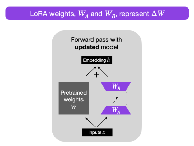
As illustrated in the figure below from the paper, LoRA leverages this by introducing two trainable low-rank matrices, \(A\) and \(B\), which capture the adaptation. \(A\) (the down-projection matrix) projects the input into a lower-dimensional subspace, while \(B\) (the up-projection matrix) maps it back to the original dimension. Per the LoRA paper by Hu et al. (2021), the matrix \(A\) is initialized with random Gaussian noise (i.i.d. samples from a normal distribution), while the matrix \(B\) is initialized to zeros so that \(\Delta W = B A\) starts as the zero matrix. During training, the product of \(A\) and \(B\) forms a low-rank update matrix that is added to the original, pre-trained weight matrix \(W\) to produce the adapted model output \(h\). This approach allows for efficient adaptation by modifying only a small subset of parameters while keeping the pre-trained weights \(W\) frozen.
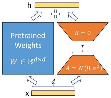
- This product, \(BA\), is low-rank because the rank of a matrix product is at most the minimum rank of the two factors. For instance, if \(B\) is a \(d \times r\) matrix and \(A\) is an \(r \times d\) matrix, where \(r\) is much smaller than \(d\), the resulting product \(BA\) will have a maximum rank of \(r\), regardless of the dimensions of \(d\). This means the update to \(W\) is constrained to a lower-dimensional space, efficiently capturing the essential information needed for adaptation.
- For example, if \(d = 1000\) and \(r = 2\), the update matrix \(BA\) will have a rank of at most 2 (since the rank of a product cannot exceed the rank of its factors), significantly reducing the number of parameters and the computational overhead required for fine-tuning. This means \(BA\) is a low-rank approximation that captures only the most essential directions needed for adaptation, thus enabling efficient updates without full matrix adjustments while keeping the pre-trained weights \(W\) frozen.
- Process:
- LoRA fundamentally changes the approach to fine-tuning large neural networks by introducing a method to decompose high-dimensional weight matrices into lower-dimensional forms, preserving essential information while reducing computational load. Put simply, LoRA efficiently fine-tunes large-scale neural networks by introducing trainable low-rank matrices, simplifying the model’s complexity while retaining its robust learning capabilities.
- LoRA is similar to methods like Principal Component Analysis (PCA) and Singular Value Decomposition (SVD), leveraging the observation that weight updates during fine-tuning are often rank-deficient. By imposing a low-rank constraint on these updates, LoRA enables a lightweight adaptation process that captures the most critical directions or “components” in the weight space. This means the model can retain essential knowledge from its pre-training phase while focusing on the specific nuances of the new task, resulting in efficient adaptation with a smaller memory and computational footprint.
- During backpropagation, only the low-rank LoRA matrices (A and B) receive gradient updates; the original pretrained weights remain frozen. Gradients flow through the combined effective weight (W = W_0 + BA), but only the LoRA-specific parameters (A and B) have
requires_grad=True, ensuring that only these low-rank components are optimized while the base model weights remain unchanged.
- Application:
- LoRA’s primary application is in the efficient fine-tuning of large neural networks, particularly in transformer-based architectures. In practice, LoRA identifies key dimensions within the original weight matrix that are crucial for a specific task, significantly reducing the adaptation’s dimensionality.
- Instead of fine-tuning all weights, which is computationally prohibitive for large models, LoRA introduces two trainable low-rank matrices, \(A\) and \(B\), in specific layers of the transformer (e.g., in the query and value projections of the attention mechanism). These matrices are optimized during training while keeping the core model parameters frozen. This architecture adjustment means that only a fraction of the original parameters are actively updated, thus lowering memory usage and enabling faster computations.
- By focusing only on the most relevant dimensions for each task, LoRA enables the deployment of large models on hardware with limited resources and facilitates task-switching by updating only the low-rank matrices without retraining the entire model.
- Benefits:
- LoRA provides several advantages that make it particularly suitable for practical use in industry and research settings where resource constraints are a concern. The primary benefit is in memory and computational efficiency.
- By keeping the majority of the model’s parameters frozen and only updating the low-rank matrices, LoRA significantly reduces the number of trainable parameters, leading to lower memory consumption and faster training times. This reduction in training complexity also means that fewer GPUs or lower-spec hardware can be used to fine-tune large models, broadening accessibility.
- Additionally, LoRA avoids introducing any additional latency during inference because, once the low-rank matrices have been trained, they can be merged back into the pre-trained weights without altering the architecture.
- This setup makes LoRA ideal for environments where models need to switch between tasks frequently, as only the task-specific low-rank weights need to be loaded, allowing the model to quickly adapt to new tasks or datasets with minimal overhead.
- In Summary:
- LoRA represents a highly efficient approach to fine-tuning, striking a balance between the depth of knowledge encapsulated in large pre-trained models and the need for targeted adaptation to new tasks or data.
- By leveraging the low intrinsic rank of weight updates, LoRA retains the model’s robustness and generalization capability while allowing for quick, cost-effective adaptations. This approach redefines efficiency in the era of massive LLMs, making it feasible to use and adapt large-scale pre-trained models across various applications and domains without the extensive computational burden associated with traditional fine-tuning.
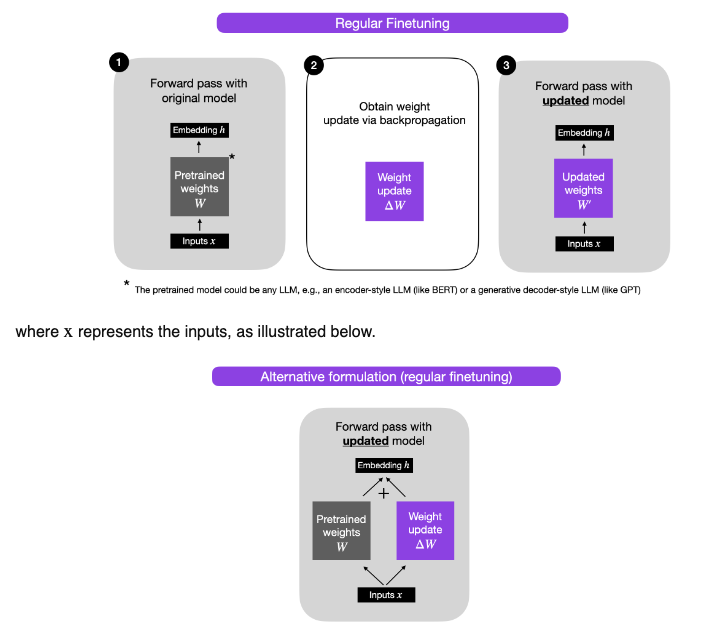
- As a recap of traditional finetuning vs. LoRA (source):
- LoRA Without Regret by John Schulman of Thinking Machines shows that, when applied to all layers with the right hyperparameters, LoRA can match full fine-tuning in performance and sample efficiency across most post-training scenarios while being significantly more compute- and memory-efficient.
Advantages
Parameter Efficiency
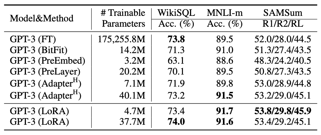
- Compared to full fine-tuning GPT-3 175B with Adam, LoRA can reduce the number of trainable parameters by 10,000 times. Specifically, this means that LoRA only fine-tunes approximately 0.01% of the parameters of the original model.
- The below table from the LoRA paper indicates that for GPT-3 with LoRA, we see that we only fine-tune \(\frac{4.7}{175255} \times 100 = 0.002\%\) and \(\frac{38}{175255} \times 100 = 0.02\%\) parameters.
GPU Memory (and Storage) Savings
- Compared to full fine-tuning GPT-3 175B with Adam, LoRA can reduce the GPU memory requirement by 3 times. Specifically, this means that LoRA fine-tunes the original model with 33% of the memory.
- For a large Transformer trained with Adam, LoRA reduces VRAM usage by up to two-thirds by avoiding the need to store optimizer states for the frozen parameters. On GPT-3 175B, VRAM consumption during training drops from 1.2TB to 350GB. When adapting only the query and value projection matrices with a rank \(r = 4\), the checkpoint size decreases significantly from approximately 350GB to 35MB. This efficiency allows training with significantly fewer GPUs and avoids I/O bottlenecks.
Efficient Task Switching
- Task switching is more cost-effective as only the LoRA weights need swapping, enabling the creation of numerous customized models that can be dynamically swapped on machines storing the pre-trained weights in VRAM.
Faster Training Speed
- Training speed also improves by 25% compared to full fine-tuning, as the gradient calculation for the vast majority of the parameters is unnecessary.
No additional inference latency
- LoRA ensures no additional inference latency when deployed in production by allowing explicit computation and storage of the combined weight matrix \(W = W_0 + BA\). During inference, this approach uses the pre-computed matrix \(W\), which includes the original pre-trained weights \(W_0\) and the low-rank adaptation matrices \(B\) and \(A\). This method eliminates the need for dynamic computations during inference.
- When switching to another downstream task, the pre-trained weights \(W_0\) can be quickly restored by subtracting the current low-rank product \(BA\) and adding the new task-specific low-rank product \(B' A'\). This operation incurs minimal memory overhead and allows for efficient task switching without impacting inference speed. By merging the low-rank matrices with the pre-trained weights in advance, LoRA avoids the extra computational burden during real-time inference (unlike adapters), ensuring latency remains on par with that of fully fine-tuned models.
Limitations
- While LoRA offers significant advantages in terms of parameter efficiency and memory savings, it also has some limitations. One notable limitation is the complexity involved in batching inputs for different tasks when using distinct low-rank matrices \(A\) and \(B\). If the goal is to absorb \(A\) and \(B\) into the combined weight matrix \(W\) to avoid additional inference latency, it becomes challenging to batch inputs from different tasks in a single forward pass. This is because each task would require a different set of \(A\) and \(B\) matrices, complicating the batching process.
- Additionally, although it is possible to avoid merging the weights and dynamically select the appropriate LoRA modules for each sample in a batch, this approach is more feasible in scenarios where latency is not a critical concern. This workaround does not fully address the need for seamless integration when low-latency inference is required across multiple tasks.
- In summary, while LoRA provides a highly efficient adaptation method, the complexity in handling multiple tasks simultaneously and the need for careful management of low-rank matrices during batching are important considerations for its practical deployment.
Hyperparameters
- LoRA-specific hyperparameters include rank (\(r\)) and alpha (\(\alpha\)). Others, while still used for LoRA-based fine-tuning, such as learning rate (lr), dropout probability (\(p\)), and batch size (\(N\)), are more generic to deep learning-based model training/fine-tuning. Here’s a detailed explanation of each:
Rank (\(r\))
-
Description: In LoRA, instead of fine-tuning the full weight matrix, the weight updates are modeled as a low-rank approximation. Specifically, the weight update matrix \(\Delta W\) is decomposed into two smaller matrices, \(A \in \mathbb{R}^{d \times r}\) and \(B \in \mathbb{R}^{r \times k}\), where \(r\) is much smaller than \(d\) or \(k\). The rank (\(r\)) of matrices \(A\) and \(B\) – one of the core hyperparameters in LoRA – represents the rank of the low-rank decomposition applied to the weight matrices. The new weight is then modeled as:
\[W = W_0 + \Delta W = W_0 + A \cdot B\] - Role: The rank controls the dimensionality of the low-rank matrices and hence the number of additional parameters introduced during fine-tuning.
-
Interpretation: Lower values of \(r\) will impose stronger restrictions on how much the weight matrices can adapt, potentially limiting the model’s flexibility but greatly reducing the computational and memory footprint. Higher values of \(r\) allow for more expressive updates but increase the number of parameters and computation required.
-
Equation: In matrix form, for any original weight matrix \(W_0 \in \mathbb{R}^{d \times k}\), the adapted weight update is expressed as:
\[\Delta W = A \cdot B\]- where, \(A \in \mathbb{R}^{d \times r}\) and \(B \in \mathbb{R}^{r \times k}\), where \(r \ll d, k\).
-
Typical Values: 2–16, depending on the size of the model and the complexity of the task. In most tasks, a small rank (e.g., 4 or 8) provides a good trade-off between performance and efficiency.
-
Higher Values: For more complex tasks, larger models, or cases where the pretrained model diverges significantly from the specialized task, higher rank values (e.g., 32, 64, or 128) may be used. Examples include:
- Adapting a general language model to legal contract review, where formal, domain-specific syntax and terminology dominate.
- Fine-tuning for biomedical question answering or clinical note summarization, which involves specialized jargon not well represented in general corpora.
- Tuning for code generation in a low-resource or proprietary programming language.
-
Adapting to historical or archaic language for cultural heritage and digitization tasks.
- These scenarios benefit from higher-rank LoRA modules due to the substantial gap between the pretraining data and the target domain, requiring more capacity to learn meaningful adaptations.
Scaling Factor (\(\alpha\))
-
Description: \(\alpha\) is a scaling factor applied to the LoRA updates. Specifically, it scales the low-rank updates \(A \cdot B\) before adding them to the base weight matrix \(W_0\). The weight update rule becomes:
\[W = W_0 + \frac{\alpha}{r} \cdot (A \cdot B)\] -
Role: The purpose of \(\alpha\) is to control the magnitude of the low-rank updates to prevent the model from diverging too far from the pre-trained weights. By dividing \(\alpha\) by the rank \(r\), LoRA ensures that the update magnitude is normalized according to the size of the low-rank decomposition. This is crucial because a larger rank would introduce more freedom for updates, and the division by \(r\) keeps the updates in check.
-
Interpretation: A higher \(\alpha\) means that the low-rank updates will have a larger impact on the final weight, while a smaller \(\alpha\) means the low-rank updates will contribute less to the adapted model. The division by \(r\) helps keep the effect of the low-rank update consistent across different choices of rank.
-
Equation: The weight update is now written as:
\[\Delta W = \frac{\alpha}{r} \cdot (A \cdot B)\] -
Typical Values: Common values for \(\alpha\) are in the range of 1–32. The typical recommendation is to set \(\alpha = \frac{r}{\text{base rank}}\), where \(\text{base rank}\) is a predetermined scale for the model.
Dropout Probability (\(p\))
-
Description: Dropout is a regularization technique used to prevent overfitting, and it is applied in the LoRA framework as well. The dropout probability (\(p\)) refers to the probability with which a particular element in the low-rank matrices \(A\) and \(B\) is randomly set to zero during training. Dropout is typically used to reduce overfitting by introducing noise during training.
-
Role: The role of dropout in LoRA is to regularize the low-rank weight updates and ensure they do not overfit to the fine-tuning data. By randomly zeroing out parts of the matrices, the model learns more robust and generalizable updates.
-
Interpretation: Higher values of dropout probability \(p\) imply more aggressive regularization, which can reduce overfitting but also may slow down learning. Lower values of \(p\) imply less regularization and could potentially lead to overfitting on small datasets.
-
Equation: The dropout operation is typically represented as:
\[A_{dropped} = A \odot \text{Bernoulli}(1-p)\]- where, \(\odot\) denotes element-wise multiplication, and \(\text{Bernoulli}(1-p)\) is a binary mask where each element is independently drawn from a Bernoulli distribution with probability \(1 - p\).
-
Typical Values: Dropout probabilities \(p\) are typically set between 0.0 (no dropout) and 0.3 for LoRA tasks.
-
Learning Rate (\(\eta\))
-
Description: The learning rate is a fundamental hyperparameter in any optimization process, and it determines the step size at which the model’s parameters are updated during training. In the context of LoRA, it controls the update of the low-rank matrices \(A\) and \(B\) rather than the full model weights.
-
Role: The learning rate governs how fast or slow the low-rank matrices adapt to the new task. A high learning rate can lead to faster convergence but risks overshooting the optimal solution, while a small learning rate can provide more stable convergence but might take longer to adapt to the new task.
-
Interpretation: A higher learning rate might be used in the early stages of fine-tuning to quickly adapt to the new task, followed by a lower rate to refine the final performance. However, too high a learning rate may destabilize training, especially when \(\alpha\) is large.
-
Equation: The update to the low-rank parameters follows the standard gradient descent update rule:
\[\theta_{t+1} = \theta_t - \eta \cdot \nabla_{\theta} L\]Where \(L\) is the loss function, \(\nabla_{\theta} L\) is the gradient of the loss with respect to the low-rank parameters \(\theta\), and \(\eta\) is the learning rate.
-
Typical Values: Learning rates for LoRA typically range from \(10^{-5}\) to \(10^{-3}\), depending on the model, the task, and the scale of adaptation needed.
-
Batch Size (\(N\))
-
Description: The batch size is the number of examples that are passed through the model at one time before updating the weights. It is a crucial hyperparameter for stabilizing the training process.
-
Role: In LoRA, the batch size affects how stable and efficient the low-rank adaptation process is. A larger batch size can stabilize the gradient estimates and speed up convergence, while smaller batches introduce more noise into the gradient, which may require a smaller learning rate to maintain stability.
-
Interpretation: Smaller batch sizes allow for faster updates but with noisier gradients, whereas larger batch sizes reduce noise but require more memory. Finding the right balance is important for both computational efficiency and effective adaptation.
-
Equation: The loss for a given batch of size \(N\) is averaged over the batch:
\[L_{\text{batch}} = \frac{1}{N} \sum_{i=1}^{N} L_i\]- where, \(L_i\) is the loss for the \(i\)-th example in the batch.
-
Typical Values: Batch sizes can vary widely depending on the available hardware resources. Typical values range from 8 to 64.
-
Summary
- The main hyperparameters involved in LoRA—rank (\(r\)), alpha (\(\alpha\)), dropout probability (\(p\)), learning rate (\(\eta\)), and batch size (\(N\))—are crucial for controlling the behavior and effectiveness of LoRA. By adjusting these parameters, LoRA can offer an efficient way to fine-tune large pre-trained models with significantly reduced computational costs and memory usage while maintaining competitive performance. Each of these hyperparameters impacts the trade-off between model flexibility, computational efficiency, and training stability.
- These hyperparameters are interconnected, especially scaling factor and rank; changes in one can require adjustments in others; more on this in the section on Is There a Relationship Between Setting Scaling Factor and Rank in LoRA?. Effective tuning of these parameters is critical for leveraging LoRA’s capabilities to adapt large models without extensive retraining.
How does having a low-rank matrix in LoRA help the fine-tuning process?
- In LoRA, a low-rank matrix is a matrix with a rank significantly smaller than its full dimensionality, which enables efficient and focused adjustments to model parameters. This lightweight adaptation mechanism allows large LLMs to learn new tasks without overfitting by capturing only the most essential adjustments, thus optimizing both information representation and parameter efficiency.
What is a Low-rank Matrix?
- A matrix is considered low-rank when its rank (the number of independent rows or columns) is much smaller than its dimensions. For example, a 1000x1000 matrix with rank 10 is low-rank because only 10 of its rows or columns contain unique information, and the others can be derived from these. This smaller rank indicates that the matrix contains a limited variety of independent patterns or directions, meaning it has a reduced capacity to capture complex relationships.
Low-Rank in LoRA Context
- In LoRA, low-rank matrices are introduced to fine-tune large LLMs with fewer trainable parameters. Here’s how it works:
- Adding Low-Rank Matrices: LoRA adds small, low-rank matrices to the model’s layers (typically linear or attention layers). These matrices serve as “adaptation” layers that adjust the original layer’s output.
- Freezing the Original Weights: The original model weights remain frozen during fine-tuning. Only the low-rank matrices are trained, which reduces the number of parameters to update.
- By limiting the rank of these new matrices, LoRA effectively limits the number of patterns they can represent. For instance, a rank-5 matrix in a high-dimensional space can only capture 5 independent directions, which forces the model to learn only essential, low-dimensional adjustments without becoming too complex.
Example
- Suppose we have a pre-trained model layer represented by a 512x512 matrix (common in large LLMs). Instead of fine-tuning this large matrix directly, LoRA adds two low-rank matrices, \(A\) and \(B\), with dimensions 512x10 and 10x512, respectively. Here:
- The product \(A \times B\) has a rank of 10, much smaller than 512.
- This product effectively adds a low-rank adaptation to the original layer, allowing it to adjust its output in just a few key directions (10 in this case), rather than making unrestricted adjustments.
Why rank matters
- The rank of the LoRA matrices directly affects the model’s ability to learn task-specific patterns:
- Lower Rank: Imposes a strong constraint on the model, which helps it generalize better and reduces the risk of overfitting.
- Higher Rank: Provides more flexibility but also increases the risk of overfitting, as the model can learn more complex adjustments that may fit the fine-tuning data too closely.
How does low-rank constraint introduced by LoRA inherently act as a form of regularization, especially for the lower layers of the model?
- In LoRA, the low-rank constraint serves as a built-in regularization mechanism by limiting the model’s flexibility during fine-tuning. This constraint especially impacts lower layers, which are designed to capture general, foundational features. By further restricting these layers, LoRA minimizes their adaptation to task-specific data, reducing the risk of overfitting. This regularization preserves the model’s foundational knowledge in the lower layers, while allowing the higher layers—where task-specific adjustments are most beneficial—to adapt more freely.
Low-Rank Constraint as Regularization
-
Low-Rank Matrices Limit Complexity: By adding only low-rank matrices to the model’s layers, LoRA restricts the model’s capacity to represent highly complex, task-specific patterns. A low-rank matrix has fewer independent “directions” or dimensions in which it can vary. This means that the model, even when fine-tuned, can only make adjustments within a constrained range, learning broad, generalizable patterns rather than memorizing specific details of the training data. This limited capacity serves as a form of regularization, preventing the model from overfitting.
-
Reduced Sensitivity to Noisy Patterns: Low-rank matrices inherently ignore minor or highly detailed variations in the training data, focusing only on dominant, overarching patterns. This makes LoRA less sensitive to the idiosyncrasies of the fine-tuning dataset, enhancing the model’s robustness and generalization ability.
Effect on Lower Layers
- The lower layers of a neural network, especially in a transformer model, are primarily responsible for extracting general-purpose features from the input data. In LLMs, for example:
- Lower layers capture basic syntactic relationships, such as sentence structure and word dependencies.
- These layers learn representations that are widely applicable across tasks and domains.
- Because these lower layers are already optimized to represent broad, generalizable patterns from pre-training, they are naturally less flexible and more constrained in what they capture compared to higher layers, which focus on more task-specific details. Adding a low-rank constraint in LoRA further reinforces this effect:
-
Enhanced Regularization on Lower Layers: Since lower layers are already constrained to capture only general patterns, the addition of a low-rank constraint essentially adds a second layer of regularization. This means that these layers become even less likely to adapt in ways that would compromise their general-purpose functionality. The low-rank constraint reinforces their role as foundational feature extractors, preserving their generalization capability while preventing overfitting on the specific details of the fine-tuning data.
-
Minimal Disruption of Pre-Trained Knowledge: The low-rank adaptation in LoRA ensures that lower layers maintain the knowledge they acquired during pre-training. Because these layers are regularized by the low-rank constraint, they are less likely to overfit to new data patterns introduced during fine-tuning. This preservation of pre-trained knowledge is crucial for maintaining the model’s transferability to other tasks or domains, as lower layers retain their broad, foundational representations.
Why This Matters for Generalization
- When fine-tuning with LoRA:
- Higher Layers Adapt More Easily: Higher layers, being closer to the output, are more adaptable and can more readily accommodate task-specific changes introduced during fine-tuning.
- Lower Layers Remain Generalized: Lower layers, reinforced by the low-rank constraint, retain their focus on general patterns. This balanced approach helps the model generalize well to unseen data because the lower layers still provide robust, general-purpose representations while the higher layers adapt to the new task.
How does LoRA help avoid catastrophic forgetting?
-
LoRA helps prevent catastrophic forgetting by fine-tuning large pre-trained models in a way that preserves their foundational knowledge while allowing for task-specific adaptations. Catastrophic forgetting occurs when fine-tuning neural networks, particularly large pre-trained models, causes them to overwrite or disrupt previously learned information, reducing performance on earlier tasks. LoRA mitigates this risk through a few key strategies:
- Freezing Original Weights: The core model parameters remain untouched, preserving the base knowledge and preventing interference.
- Introducing Low-Rank Matrices: These matrices have limited capacity, focusing solely on task-specific adjustments, which allows the model to adapt to new tasks without losing general knowledge.
- Targeting Specific Layers: LoRA typically modifies higher attention layers, avoiding disruption to fundamental representations in lower layers.
- Parameter-Efficient, Modular Adaptation: LoRA’s modular design allows for reversible, task-specific adjustments, making it suitable for flexible multi-task and continual learning.
-
Through this approach, LoRA enables large models to adapt efficiently to new tasks while retaining previously learned information, which is especially valuable for applications requiring retention of prior knowledge.
Freezing the Original Weights
- One of the core aspects of LoRA is that it freezes the original model weights and adds new, low-rank matrices that handle the fine-tuning process:
- The frozen original weights retain the model’s general knowledge from pre-training. This means that core information, patterns, and representations acquired from extensive pre-training on large datasets remain unaffected.
- Since only the low-rank matrices are adjusted for the new task, there is no direct modification of the original weights. This minimizes the risk of overwriting or disrupting the knowledge captured in those weights.
- By keeping the original parameters intact, LoRA avoids catastrophic forgetting in a way that typical fine-tuning (where the original weights are updated) does not.
Low-Rank Adaptation Layers for Task-Specific Adjustments
- LoRA introduces low-rank matrices as additional layers to the model, which have the following properties:
- Limited Capacity: Low-rank matrices have a constrained capacity to represent new information, which forces them to focus only on essential, task-specific adaptations. This means they cannot significantly alter the underlying model’s behavior, preserving the broader general knowledge.
- Focused Adaptation: By adding task-specific information via low-rank matrices rather than altering the model’s entire parameter space, LoRA ensures that the new task-specific changes are confined to these auxiliary matrices. This helps the model adapt to new tasks without losing its prior knowledge.
Layer-Specific Impact
- LoRA often targets specific layers in the model, commonly the attention layers:
- Higher Attention Layers: These layers (closer to the output) are responsible for more task-specific representations and are typically the ones modified by LoRA. This selective adaptation means that the deeper, more task-general features in lower layers are left intact, reducing the risk of catastrophic forgetting.
- Minimal Lower-Layer Impact: Since lower layers (closer to the input) remain unchanged or minimally affected, the model retains the general-purpose, foundational features learned during pre-training, which are crucial for generalization.
- This selective impact allows LoRA to introduce new, task-specific representations while preserving fundamental information, balancing new task learning with knowledge retention.
Parameter-Efficient Fine-Tuning
- LoRA is designed for parameter-efficient fine-tuning, meaning it uses a fraction of the parameters that traditional fine-tuning would require:
- LoRA adds only a small number of new parameters through the low-rank matrices. This efficiency keeps the model changes lightweight, making it less likely to interfere with the original model’s representations.
- The low-rank constraint also regularizes the fine-tuning process, helping to prevent overfitting to the new task, which can indirectly support retention of general knowledge. Overfitting can cause catastrophic forgetting if the model becomes too specialized, as it loses flexibility in dealing with tasks beyond the fine-tuning data.
Easy Reversibility
- Since LoRA’s approach is to add new matrices rather than alter the original model’s weights, it makes it easy to revert the model to its original state or apply it to different tasks:
- The low-rank matrices can be removed or swapped out without affecting the base model. This modularity allows for rapid switching between tasks or models, making it easy to adapt the model to different tasks while maintaining the pre-trained knowledge.
- This adaptability is particularly useful for multi-task learning or continual learning, as it allows LoRA-enhanced models to apply distinct low-rank adaptations for different tasks without compromising the model’s underlying pre-trained knowledge.
Modular and Reusable Adapters
- With LoRA, fine-tuning for different tasks can be achieved by creating different low-rank matrices for each new task:
- These modular, reusable matrices enable task-specific tuning without overwriting previous adaptations or the original model. This is especially valuable for applications where the model needs to perform multiple tasks or domains interchangeably.
- By associating each task with its own set of low-rank matrices, LoRA enables the model to maintain knowledge across tasks without interference, effectively circumventing catastrophic forgetting.
How does multiplication of two low-rank matrices in LoRA lead to lower attention layers being impacted less than higher attention layers?
- In LoRA, the use of low-rank matrices enables efficient, controlled updates by selectively applying them to specific layers—primarily in the higher attention layers rather than the lower ones. This targeted approach allows the model to adjust effectively to task-specific nuances in these higher layers, which capture more complex patterns and contextual information, while preserving the general features encoded in the lower layers. By focusing fine-tuning efforts on the higher layers, LoRA minimizes overfitting and retains foundational knowledge from pre-training, making it an efficient and effective fine-tuning strategy.
Role of Low-Rank Matrices in LoRA
- LoRA adds two low-rank matrices, \(A\) and \(B\), to certain layers, typically in the form:
\(W_{\text{new}} = W + A \times B\)
- where:
- \(W\) is the original (frozen) weight matrix in the model layer.
- \(A\) and \(B\) are low-rank matrices (with ranks much smaller than the original dimensionality of \(W\)), creating a low-rank adaptation.
- where:
- The product \(A \times B\) has a limited rank and thus introduces only a restricted adjustment to \(W\). This adjustment constrains the layer to learn only a few independent patterns rather than a full set of complex, task-specific transformations.
Higher Attention Layers: Task-Specific Focus
- In large models, higher attention layers (closer to the output) tend to capture task-specific, abstract features, while lower attention layers (closer to the input) capture general, reusable patterns. By applying LoRA-based fine-tuning primarily to higher attention layers:
- The model’s low-rank adaptation focuses on high-level, task-specific adjustments rather than modifying general representations.
- Higher layers, which already deal with more specific information, are more sensitive to the small adjustments made by \(A \times B\) since they directly influence task-related outputs.
- In practice, LoRA-based fine-tuning modifies these higher layers more significantly because these layers are more directly responsible for adapting the model to new tasks. Lower layers, in contrast, require less task-specific adjustment and retain their general-purpose features.
Limited Capacity of Low-Rank Matrices and Layer Impact
- The low-rank matrices \(A\) and \(B\) have limited expressive power (due to their low rank), meaning they can only introduce a small number of directional adjustments in the weight space. This limited capacity aligns well with higher layers because:
- Higher layers don’t need drastic changes but rather subtle adjustments to fine-tune the model to specific tasks.
- The constraint imposed by low-rank matrices helps avoid overfitting by restricting the number of learned patterns, which is ideal for the high-level, abstract representations in higher layers.
- For lower layers, which capture broad, general-purpose features, such limited adjustments don’t significantly impact the model. Lower layers still operate with the general features learned during pre-training, while higher layers adapt to task-specific details.
Why Lower Layers are Less Affected
- Lower layers in the attention stack are less impacted by LoRA’s low-rank updates because:
- They are often not fine-tuned at all in LoRA-based setups, preserving the general features learned during pre-training.
- Even when fine-tuned with low-rank matrices, the limited capacity of \(A \times B\) is not sufficient to drastically alter their broader, foundational representations.
In LoRA, why is \(A\) initialized using a Gaussian and \(B\) set to 0?
- In LoRA, the initialization strategy where matrix \(A\) is initialized with a Gaussian distribution and matrix \(B\) is set to zero is crucial for ensuring a smooth integration of the adaptation with minimal initial disruption to the pre-trained model. This approach is designed with specific goals in mind:
Preserving Initial Model Behavior
- Rationale: By setting \(B\) to zero, the product \(\Delta W = BA\) initially equals zero. This means that the adapted weights do not alter the original pre-trained weights at the beginning of the training process.
- Impact: This preserves the behavior of the original model at the start of fine-tuning, allowing the model to maintain its pre-trained performance and stability. The model begins adaptation from a known good state, reducing the risk of drastic initial performance drops.
Gradual Learning and Adaptation
- Rationale: Starting with \(\Delta W = 0\) allows the model to gradually adapt through the updates to \(B\) during training. This gradual adjustment is less likely to destabilize the model than a sudden, large change would.
- Impact: As \(B\) starts updating from zero, any changes in the model’s behavior are introduced slowly. This controlled adaptation is beneficial for training dynamics, as it allows the model to incrementally learn how to incorporate new information effectively without losing valuable prior knowledge.
Ensuring Controlled Updates
- Rationale: Gaussian initialization of \(A\) provides a set of initial values that, while random, are statistically regularized by the properties of the Gaussian distribution (such as having a mean of zero and a defined variance). This regularity helps in providing a balanced and predictable set of initial conditions for the adaptation process.
- Impact: The Gaussian distribution helps ensure that the values in \(A\) are neither too large nor too biased in any direction, which could lead to disproportionate influence on the updates when \(B\) begins to change. This helps in maintaining a stable and effective learning process.
Focused Adaptation
- Rationale: The low-rank matrices \(A\) and \(B\) are intended to capture the most essential aspects of the new data or tasks relative to the model’s existing capabilities. By starting with \(B = 0\) and \(A\) initialized randomly, the learning focuses on identifying and optimizing only those aspects that truly need adaptation, as opposed to re-learning aspects that the model already performs well.
-
Impact: This focus helps optimize training efficiency by directing computational resources and learning efforts towards making meaningful updates that enhance the model’s capabilities in specific new areas.
- This initialization strategy supports the overall goal of LoRA: to adapt large, pre-trained models efficiently with minimal resource expenditure and without compromising the foundational strengths of the original model. This approach ensures that any new learning builds on and complements the existing pre-trained model structure.
For a given task, how do we determine whether to fine-tune the attention layers or feed-forward layers?
- Deciding whether to fine-tune the attention layers or the feed-forward (MLP) layers in a model adapted using LoRA involves several considerations. These include the nature of the task, the model architecture, and the distribution of parameters between attention and feed-forward layers.
- Note that the LoRA paper originally only adapted the attention weights for downstream tasks and froze the MLP modules (so they are not trained in downstream tasks) both for simplicity and parameter-efficiency. Thus, the number of attention weights relative to feed-forward weights can impact the choice of .
- Here are some key factors to guide this decision:
Nature of the Task
- Task Requirements: Attention mechanisms are particularly effective for tasks that benefit from modeling relationships between different parts of the input, such as sequence-to-sequence tasks or tasks requiring contextual understanding. If the task demands strong relational reasoning or context sensitivity, fine-tuning attention layers might be more beneficial.
- Feed-Forward Layer Role: MLPs generally focus on transforming the representation at individual positions without considering other positions. They are effective for tasks requiring more substantial non-linear transformation of features. If the task demands significant feature transformation at individual positions, MLPs may need adaptation.
Model Architecture
- Proportion of Parameters: In transformer architectures, MLPs typically contain a larger number of parameters compared to attention mechanisms (of the order of 2x to 5x). For example, in standard configurations like those seen in BERT or GPT models, the MLPs can contain around three times more parameters than the attention layers.
- Impact on Efficiency: Because MLPs are parameter-heavy, fine-tuning them can significantly increase the number of trainable parameters, impacting training efficiency and computational requirements. If parameter efficiency is a priority, you might opt to adapt only the attention layers, as originally done in the LoRA approach.
Computational Constraints
- Resource Availability: The decision can also be influenced by available computational resources. Adapting attention layers only can save computational resources and training time, making it a preferable option when resources are limited.
- Balance of Adaptation and Performance: If computational resources allow, experimenting with both components can be useful to understand which contributes more to performance improvements on specific tasks.
Empirical Testing
- A/B Testing: One effective way to determine the optimal strategy for a specific model and task is to conduct empirical tests where you fine-tune the attention layers alone, the MLP layers alone, and both together in different experiments to compare the performance impacts.
- Performance Metrics: Monitoring key performance metrics specific to the task during these tests will guide which components are more critical to fine-tune.
Task-Specific Research and Insights
-
Literature and Benchmarks: Insights from research papers and benchmarks on similar tasks can provide guidelines on what has worked well historically in similar scenarios. For example, tasks that require nuanced understanding of input relationships (like question answering or summarization) might benefit more from tuning attention mechanisms.
-
In summary, the choice between tuning attention or MLP layers depends on the specific demands of the task, the model’s architecture, the balance of parameters, and empirical results. Considering these aspects can help in making a decision that optimizes both performance and efficiency.
Assuming we’re fine-tuning attention weights, which specific attention weight matrices should we apply LoRA to?
- The question of which attention weight matrices in the transformer architecture should be adapted using LoRA to optimize performance on downstream tasks is central to maximizing the effectiveness of parameter usage, especially when dealing with large models like GPT-3. Based on the findings reported in the LoRA paper and the specific experiment mentioned, here’s a detailed explanation and recommendation:
Context and Setup
- The LoRA paper explores the adaptation of various weight matrices within the self-attention module of GPT-3 under a limited parameter budget. With a constraint of 18 million trainable parameters, the authors tested different configurations of adapting the weights associated with the query (\(W_q\)), key (\(W_k\)), value (\(W_v\)), and output (\(W_o\)) matrices. This setup allows for a comparison of the effectiveness of adapting different combinations of weights at varying ranks.
Experimental Findings
- Parameter Allocation: The experiment considered adapting individual weight types at a rank of 8 and combinations of weights at lower ranks (4 and 2) due to the fixed parameter budget. This arrangement allowed assessing whether it is more beneficial to distribute the available parameters across multiple weight types or concentrate them on fewer weights at a higher rank.
- Performance Metrics: The validation accuracies on the WikiSQL and MultiNLI datasets served as the primary performance indicators. The results show varying degrees of success depending on which weights were adapted and how the ranks were distributed. The table below from the LoRA paper shows validation accuracy on WikiSQL and MultiNLI after applying LoRA to different types of attention weights in GPT-3, given the same number of trainable parameters. Adapting both \(W_q\) and \(W_v\) gives the best performance overall. They find the standard deviation across random seeds to be consistent for a given dataset, which they report in the first column.
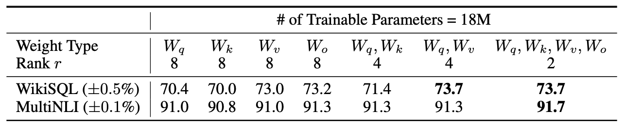
Key Results and Recommendations
- Single vs. Multiple Weight Adaptation: Adapting single weight matrices (\(W_q\), \(W_k\), \(W_v\), or \(W_o\) individually) at a higher rank generally resulted in lower performance compared to adapting combinations of weights at a reduced rank. Specifically, putting all parameters in ∆\(W_q\) or ∆\(W_k\) alone did not yield optimal results.
- Optimal Combination: The combination of adapting both \(W_q\) and \(W_v\) at a rank of 4 emerged as the most effective strategy, achieving the highest validation accuracies on both datasets. This suggests a balanced approach to distributing the parameter budget across multiple types of attention weights, rather than focusing on a single type, leads to better performance.
- Effectiveness of Rank Distribution: The result indicates that a lower rank (such as 4) is sufficient to capture essential adaptations in the weights, making it preferable to spread the parameter budget across more types of weights rather than increasing the rank for fewer weights.
Conclusion and Strategy for Applying LoRA
- Based on these findings, when applying LoRA within a limited parameter budget, it is advisable to:
- Distribute Parameters Across Multiple Weights: Focus on adapting multiple types of attention weights (such as \(W_q\) and \(W_v\)) rather than a single type, as this approach leverages the synergistic effects of adapting multiple aspects of the attention mechanism.
- Use Lower Ranks for Multiple Weights: Opt for a lower rank when adapting multiple weights to ensure that the parameter budget is used efficiently without compromising the ability to capture significant adaptations.
- This strategy maximizes the impact of the available parameters by enhancing more dimensions of the self-attention mechanism, which is crucial for the model’s ability to understand and process input data effectively across different tasks.
Is there a relationship between setting scaling factor and rank in LoRA?
- In the LoRA framework, the relationship between the scaling factor \(\alpha\) and the rank \(r\) of the adaptation matrices \(A\) and \(B\) is an important consideration for tuning the model’s performance and managing how adaptations are applied to the pre-trained weights. Both \(\alpha\) and \(r\) play significant roles in determining the impact of the low-rank updates on the model, and their settings can influence each other in terms of the overall effect on the model’s behavior.
Understanding \(\alpha\) and \(r\)
- Scaling Factor \(\alpha\): This parameter scales the contribution of the low-rank updates \(\Delta W = BA\) before they are applied to the original model weights \(W\). It controls the magnitude of changes introduced by the adaptation, effectively modulating how aggressive or subtle the updates are.
- Rank \(r\): This determines the dimensionality of the low-rank matrices \(A\) and \(B\). The rank controls the expressiveness of the low-rank updates, with higher ranks allowing for more complex adaptations but increasing computational costs and potentially the risk of overfitting.
Relationship and Interaction
- Balancing Impact: A higher rank \(r\) allows the model to capture more complex relationships and nuances in the adaptations, potentially leading to more significant changes to the model’s behavior. In such cases, \(\alpha\) might be adjusted downward to temper the overall impact, ensuring that the modifications do not destabilize the model’s pre-trained knowledge excessively.
- Adjusting for Subtlety: Conversely, if the rank \(r\) is set lower, which constrains the flexibility and range of the updates, \(\alpha\) may need to be increased to make the limited updates more impactful. This can help ensure that the adaptations, though less complex, are sufficient to achieve the desired performance improvements.
- Experimental Tuning: The optimal settings for \(\alpha\) and \(r\) often depend on the specific task, the dataset, and the desired balance between adapting to new tasks and retaining generalizability. Experimentation and validation are typically necessary to find the best combination.
Practical Considerations
- Overfitting vs. Underfitting: Higher ranks with aggressive scaling factors can lead to overfitting, especially when the model starts fitting too closely to nuances of the training data that do not generalize well. Conversely, too low a rank and/or too conservative an \(\alpha\) might lead to underfitting, where the model fails to adapt adequately to new tasks.
- Computational Efficiency: Higher ranks increase the number of parameters and computational costs. Balancing \(\alpha\) and \(r\) can help manage computational demands while still achieving meaningful model improvements.
Conclusion
- The relationship between \(\alpha\) and \(r\) in LoRA involves a delicate balance. Adjusting one can necessitate compensatory changes to the other to maintain a desired level of adaptation effectiveness without sacrificing the model’s stability or performance. Understanding how these parameters interact can significantly enhance the strategic deployment of LoRA in practical machine learning tasks.
How do you determine the optimal rank \(r\) for LoRA?
- The optimal rank \(r\) for LoRA is influenced by the specific task and the type of weight adaptation. Based on the results reported in the paper from the experiments on the WikiSQL and MultiNLI datasets:
- For WikiSQL:
- When adapting only \(W_q\), the optimal rank is \(r = 4\), with a validation accuracy of 70.5%.
- When adapting \(W_q\) and \(W_v\), the optimal rank is \(r = 8\), with a validation accuracy of 73.8%.
- When adapting \(W_q, W_k, W_v, W_o\), the optimal ranks are \(r = 4\) and \(r = 8\), both achieving a validation accuracy of 74.0%.
- For MultiNLI:
- When adapting only \(W_q\), the optimal rank is \(r = 4\), with a validation accuracy of 91.1%.
- When adapting \(W_q\) and \(W_v\), the optimal rank is \(r = 8\), with a validation accuracy of 91.6%.
- When adapting \(W_q, W_k, W_v, W_o\), the optimal ranks are \(r = 2\) and \(r = 4\), both achieving a validation accuracy of 91.7%.
- For WikiSQL:
- The table below from the paper shows the validation accuracy on WikiSQL and MultiNLI with different rank \(r\) by adapting \(\left\{W_q, W_v\right\}\), \(\left\{W_q, W_k, W_v, W_c\right\}\), and just \(W_q\) for a comparison.. To our surprise, a rank as small as one suffices for adapting both \(W_q\) and \(W_v\) on these datasets while training \(W_q\) alone needs a larger \(r\).
![]()
- In summary, while the optimal rank \(r\) varies depending on the dataset and the type of weight adaptation, a rank of \(r = 4\) or \(r = 8\) generally yields the best performance. Specifically, a rank of \(r = 4\) is often sufficient for single weight types like \(W_q\), and a rank of \(r = 8\) is more effective for adapting multiple weight types such as \(W_q\) and \(W_v\).
- However, a small \(r\) cannot be expected to work for every task or dataset. Consider the following thought experiment: if the downstream task were in a different language than the one used for pre-training, retraining the entire model (similar to LoRA with \(r = d_{model}\)) could certainly outperform LoRA with a small \(r\).
- In summary, selecting a rank that is too high can counteract the benefits of the low-rank adaptation by allowing the model to become overly complex and fit the training data too precisely. Conversely, choosing a rank that’s too low may limit the model’s ability to capture necessary information, leading to underfitting. Therefore, setting the rank in LoRA fine-tuning involves finding a balance: enough capacity to adapt to new data without overfitting.
How do LoRA hyperparameters interact with each other? Is there a relationship between LoRA hyperparameters?
-
There is a significant relationship among the hyperparameters in the Low-Rank Adaptation (LoRA) technique, particularly how they interact and influence each other to affect the adaptation and performance of the model. Understanding the interactions between these hyperparameters is crucial for effectively tuning the model to achieve desired behaviors and performance improvements. Here’s a detailed breakdown of the primary hyperparameters in LoRA and how they are interrelated:
- Rank and Scaling Factor:
- Higher ranks allow \(A\) and \(B\) to capture more detailed and complex modifications. However, with increased rank, the potential for overfitting and destabilizing the original model’s behavior also rises. The scaling factor \(\alpha\) often needs to be adjusted in response to the rank; a higher rank might require a smaller \(\alpha\) to moderate the effect of these more complex updates.
- Rank and Regularization:
- As the rank increases, the number of parameters in \(A\) and \(B\) also increases, which can lead to overfitting. Regularization becomes more critical with higher ranks to ensure that the model generalizes well and does not just memorize the training data.
- Learning Rate and Scaling Factor:
- The learning rate for \(A\) and \(B\) can influence how quickly the model adapts the low-rank updates. If \(\alpha\) is high, leading to stronger updates, a lower learning rate might be necessary to prevent training instability. Conversely, with a lower \(\alpha\), a higher learning rate might be feasible to ensure that the updates are sufficiently impactful.
- Regularization and Learning Rate:
- Regularization settings might need adjustment based on the learning rate. A higher learning rate can cause larger updates, which might increase the risk of overfitting unless balanced by stronger regularization.
Practical Considerations
- Tuning Strategy:
- Tuning these hyperparameters requires careful experimentation and validation. Often, changes to one parameter necessitate adjustments to others to maintain a balanced and effective training regime.
- Trade-offs:
- There are trade-offs between model flexibility, training stability, computational efficiency, and the risk of overfitting. Effective management of LoRA’s hyperparameters is key to navigating these trade-offs.
- Application-Specific Adjustments:
- Depending on the specific requirements of the task and characteristics of the data, the optimal settings for these hyperparameters can vary significantly. Task-specific performance metrics and validation are essential to guide these adjustments.
- In summary, understanding and managing the relationships between these LoRA hyperparameters enables practitioners to finely tune their models to specific tasks without extensive retraining while leveraging pre-trained model architectures efficiently.
Why does a higher rank make it the easier to overfit?
- In LoRA-based fine-tuning, a higher rank can indeed lead to easier overfitting. To understand why, let’s break down the mechanics of LoRA and how rank affects model capacity and overfitting.
- The rank in LoRA determines the dimensions of these additional matrices, effectively controlling their capacity to capture information:
- Low Rank: Small matrices that can represent only limited information.
- High Rank: Larger matrices with greater capacity to capture complex patterns.
-
In mathematical terms, a higher rank means more degrees of freedom in the low-rank matrices, allowing them to approximate more complex relationships in the data.
- Here’s why a higher rank increases overfitting in LoRA:
-
Increased Capacity to Capture Training Noise: A higher rank increases the expressive power of the LoRA matrices. This means they can capture not only meaningful patterns in the training data but also noise or spurious correlations. This added capacity can lead the model to “memorize” the training data rather than generalize from it, making it prone to overfitting.
-
Less Regularization Effect: Low-rank matrices act as a form of regularization by constraining the model’s capacity to learn only the most essential patterns. When the rank is increased, this regularization effect diminishes. The model can then adjust more parameters, fitting closely to the training data distribution, which can hurt its performance on unseen data.
-
Reduced Ability to Generalize: The initial idea behind LoRA is to adapt large models with minimal parameter changes to preserve generalization. By increasing the rank, we deviate from this minimalist adaptation, moving toward a more specialized adaptation to the training data. This specialization makes it harder for the model to generalize to different data distributions.
-
Higher Variance in Learned Features: With higher-rank matrices, the LoRA-based adjustments might capture a wider variety of features from the training data, leading to high variance in the learned representations. This increased variance can cause the model’s predictions to vary more significantly with small changes in the input, reducing its robustness and making it overfit the nuances of the training set.
-
Does LoRA adapt weights in all layers?
-
LoRA does not typically adapt weights across all layers of a neural network; instead, it targets specific layers, often the attention layers in large LLMs. This selective adaptation is a design choice aimed at balancing the effectiveness of fine-tuning with computational efficiency and minimizing the risk of overfitting. By modifying only key layers, like attention layers, LoRA efficiently focuses on layers where task-specific information is most impactful while preserving the general-purpose features of the lower layers.
-
Layers Typically Adapted in LoRA:
- In the original LoRA implementation:
- Attention Layers: LoRA primarily targets attention layers (such as the query and value projections in transformers) because they play a critical role in capturing contextual information. By adapting only these layers, LoRA can achieve significant task-specific improvements without needing to modify the entire model.
- Few Additional Layers (if necessary): Sometimes, LoRA may extend adaptation to a few other layers (like feed-forward layers in transformers) if the new task requires it. However, this is usually done with caution to avoid overfitting and to keep the parameter footprint low.
-
Why not all layers?:
- Computational Efficiency: Adapting all layers would introduce a large number of low-rank matrices throughout the model, greatly increasing the memory and computation requirements, which LoRA is specifically designed to reduce.
- Risk of Overfitting: Adapting all layers, especially the lower (more general) layers, could lead the model to overfit to the fine-tuning dataset, particularly if the dataset is small. Lower layers tend to capture general features, and adapting them might make the model too specialized, losing generalization ability.
- Focus on Task-Specific Information: The upper (or top) layers of a model generally capture task-specific features, while lower layers handle more general, reusable features. LoRA’s selective adaptation focuses on adjusting only those layers where task-specific learning is most beneficial.
Does LoRA impact lower attention layers less than higher attention layers?
-
Yes, in practice, LoRA impacts higher attention layers more than lower ones. This is because LoRA selectively adapts layers, targeting the task-specific adaptability of higher layers while preserving the general-purpose features in lower layers. This design enables effective task adaptation with minimal overfitting, allowing the model to retain broad applicability.
-
Why higher attention layers are more affected:
-
Function of Higher Attention Layers: Higher attention layers (those closer to the output) tend to capture more task-specific, abstract information. During fine-tuning, LoRA modifies these layers to incorporate new task-related features. Adjustments here have a greater impact on the model’s output because these layers process information in a way that directly influences final predictions.
-
Less Impact on Lower Layers: Lower layers (closer to the input) generally focus on extracting basic, general features. For example, in LLMs, they capture fundamental linguistic structures like syntax and word relationships. Since these lower layers capture foundational patterns, they benefit less from task-specific adaptations. Fine-tuning these lower layers with LoRA could lead to a loss of generalizable features, which would reduce the model’s ability to transfer across tasks.
-
LoRA’s Selective Impact: LoRA is typically implemented on a subset of attention heads or specific projections within the attention mechanism (e.g., the query and value projections). Even when applied across all layers, the task-specific nature of fine-tuning tends to have a more pronounced effect on the higher layers, which adapt more flexibly to new data patterns.
-
Regularization Effect in Lower Layers: Because LoRA introduces a low-rank constraint, it inherently acts as a form of regularization. Lower layers, which are already constrained to represent general features, become even more regularized. This further reduces the likelihood of significant changes in these layers and minimizes the effect of LoRA on them.
-
-
Practical Implications:
-
In many cases, fine-tuning with LoRA results in:
- Major adjustments to higher layers, allowing the model to learn specific features of the fine-tuning task.
- Minimal impact on lower layers, preserving general knowledge from pre-training and preventing overfitting.
Quantized Low-Rank Adaptation (QLoRA)
- Proposed in QLoRA: Efficient Finetuning of Quantized LLMs by Dettmers et al. from the University of Washington.
- QLoRA is an efficient finetuning method that enables training very large models—up to 65B parameters—on a single 48GB GPU, without loss of accuracy compared to full 16-bit finetuning. It does this by backpropagating through a frozen, 4-bit quantized pretrained model into LoRA Adapters.
- In short, QLoRA combines LoRA’s parameter-efficient adaptation with two key quantization innovations—4-bit NormalFloat (
NF4) and Double Quantization (DQ)—plus paged optimizers to handle memory spikes. This combination greatly reduces GPU memory usage while preserving performance. - For a practical introduction to QLoRA, see this Hugging Face blog on Making LLMs even more accessible with bitsandbytes, 4-bit quantization and QLoRA.
High-level process
- Quantize the pretrained model weights to 4-bit and freeze them.
- Attach small, trainable LoRA adapters throughout the transformer layers.
- Fine-tune only these adapters while the quantized base model remains frozen.
- The figure below from the paper shows different finetuning methods and their memory requirements. QLoRA improves over LoRA by quantizing the transformer model to 4-bit precision and using paged optimizers to handle memory spikes.
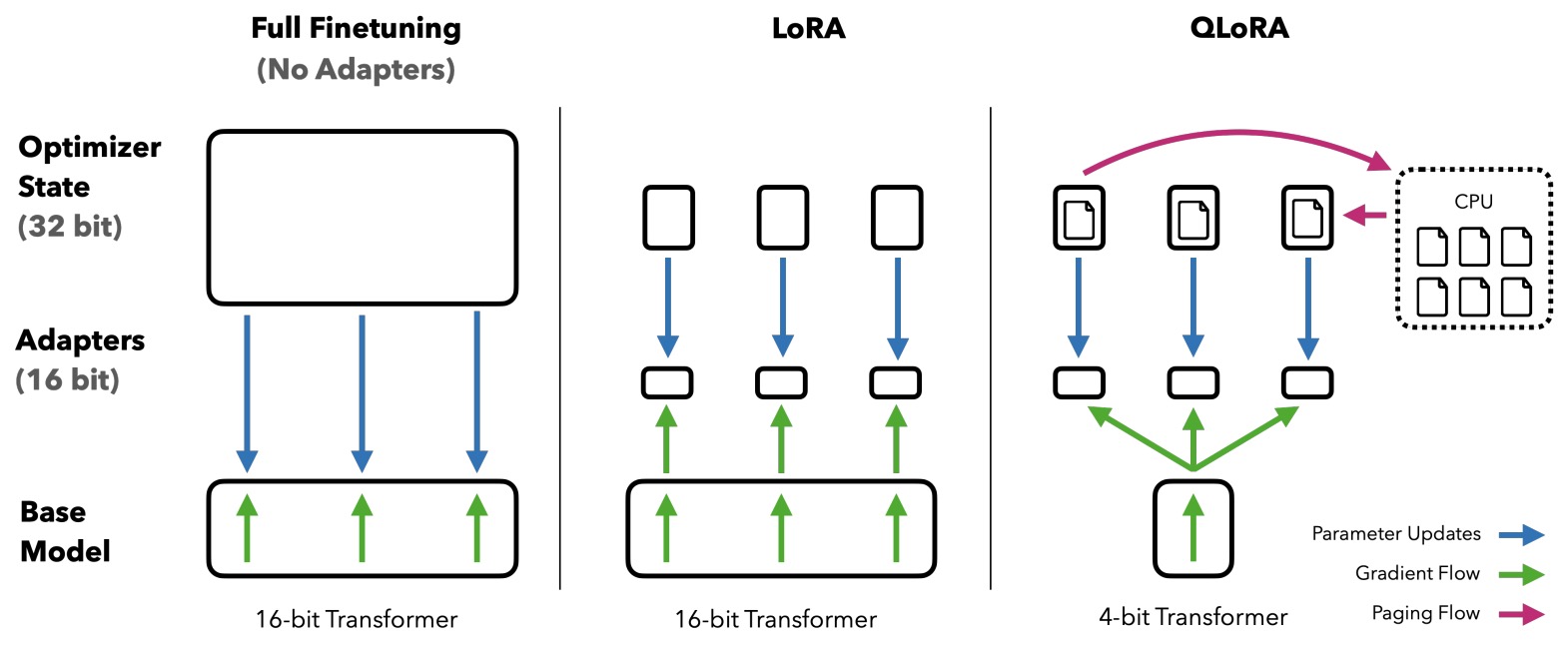
- The figure below (source) compares full fine-tuning, LoRA, and QLoRA:
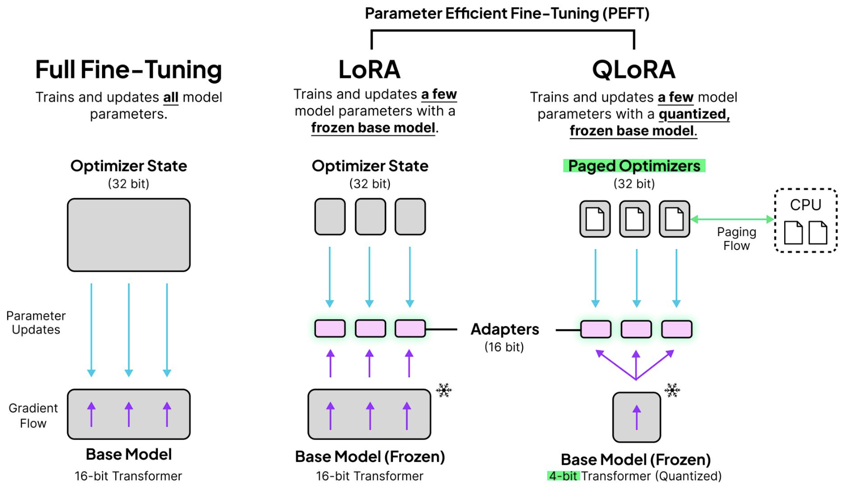
Key Components
-
Low-Rank Adaptation (LoRA):
- Inserts small rank-decomposed trainable matrices into all of a base model’s layers. Put simply, the LoRA adapters are applied to both the self-attention module (including query, key, value, and output projections)–as in vanilla LoRA–and the feed-forward network (MLP) layers inside each transformer block. This broader placement was found to be critical for matching the performance of full 16-bit finetuning.
- Only these adapters are updated; the large frozen weight matrices are never modified.
-
4-bit NormalFloat (
NF4) Quantization:NF4is an information-theoretically optimal quantization scheme for values drawn from a zero-centered normal distribution (common for pretrained LLM weights).- It is based on quantile quantization, ensuring each bin contains an equal probability mass, minimizing quantization error.
NF4avoids expensive per-tensor quantile estimation by exploiting the fact that all weights can be scaled to match a fixed \(N(0,1)\) distribution, allowing the use of precomputed quantization bin edges.- The quantization is asymmetric with an exact zero representation, which is crucial for padding/sparse elements, and means that only a scale value (no zero-point) needs to be stored for each block.
- Compared to regular 4-bit floats (
FP4),NF4yields lower perplexity and higher accuracy across benchmarks while keeping the same memory footprint.
-
Double Quantization (DQ):
- In block-wise quantization, each block of weights has an associated quantization constant (scale) — but no separate zero-point, since
NF4’s asymmetric codebook already contains an exact zero representation. These scale values are the only per-block metadata stored alongside the quantized weights, and in QLoRA’s DQ scheme, they are themselves quantized to further reduce memory overhead. For small block sizes (e.g., 64), storing these constants can be a large relative memory cost. - DQ reduces this overhead by quantizing the quantization constants themselves.
- The first quantization maps
FP32weights →NF4values with per-blockFP32scales. - The second quantization maps these scales into
FP8(block size 256), plus a second set ofFP32scales for dequantization. - This reduces quantization constant storage from 0.5 bits per parameter to 0.127 bits per parameter—a 0.373 bit saving per parameter—without measurable performance loss.
- In block-wise quantization, each block of weights has an associated quantization constant (scale) — but no separate zero-point, since
-
Paged Optimizers:
- Uses NVIDIA Unified Memory to automatically swap optimizer states between CPU RAM and GPU memory when GPU memory is full during large sequence processing.
- This avoids out-of-memory errors without slowing down training under typical sequence lengths.
Operation
-
In a single linear layer with LoRA in QLoRA:
- Stored weight format:
NF4quantized base model weights, plus LoRA adapter weights inBF16. - Computation:
- Dequantize
NF4weights (double dequantization if DQ is used) intoBF16on the fly. - Perform matrix multiplications with the dequantized weights plus LoRA projections.
- Backpropagate gradients only into LoRA parameters; no gradient storage for the base weights.
- Dequantize
In QLoRA, only the original model’s weights are quantized to
NF4. The LoRA adapter weights remain in higher precision (BF16) and are the only parameters updated during finetuning. - Stored weight format:
-
Formally:
-
Forward pass with double dequantization:
- \[W_{\text{NF4}} \xrightarrow{\text{DQ}} W_{\text{BF16}}\]
- \[Y_{\text{BF16}} = X_{\text{BF16}} \cdot W_{\text{BF16}} + X_{\text{BF16}} L_1 L_2\]
-
Backward pass:
- Compute derivatives w.r.t. LoRA parameters only, while still dequantizing base weights for intermediate computations.
-
Impact and Results
- Guanaco, the best-performing QLoRA model family, achieves 99.3% of ChatGPT’s score on the Vicuna benchmark after 24 hours of finetuning on a single GPU.
- QLoRA’s memory optimizations—
NF4, double quantization, and paged optimizers—enable training 33B parameter models on 24GB consumer GPUs and 65B models on a single 48GB GPU. - Across GLUE, Super-NaturalInstructions, and MMLU benchmarks,
NF4+ DQ matches or exceeds full 16-bit LoRA and full finetuning results, outperformingFP4andINT4quantization. - This makes large-scale finetuning accessible for small teams and researchers without massive compute clusters.
Quantization-Aware Low-Rank Adaptation (QA-LoRA)
- Proposed in QA-LoRA: Quantization-Aware Low-Rank Adaptation of Large LLMs.
- Xu et al. from Huawei propose Quantization-Aware Low-Rank Adaptation (QA-LoRA), which jointly performs parameter-efficient fine-tuning and low-bit quantization. Unlike prior methods, QA-LoRA ensures that the fine-tuned weights remain in low-bit form after training, eliminating the need for post-training quantization (PTQ) — a step that typically introduces accuracy degradation at very low bit widths such as
INT3orINT2. In standard approaches like LoRA or QLoRA, fine-tuning ends with full-precision weights (e.g.,FP16). Deploying in low precision then requires PTQ, which compresses the model after it has been optimized in high precision, leading to significant quantization error and loss in accuracy for low-bit formats. QA-LoRA avoids this by training directly in the target low-bit format in a quantization-aware manner, so the model is deployment-ready without further quantization steps. - Put simply, QA-LoRA extends QLoRA’s idea but removes its main deployment bottleneck (FP16 fallback) while improving accuracy at lower bit widths, all with minimal implementation overhead. The merged weights \(W' = \tilde{W} + sAB\) remain quantized throughout fine-tuning, meaning inference can run natively on low-bit integer kernels without precision fallback.
- The motivation comes from an imbalance between the Degrees of Freedom (DoF) of quantization and adaptation: traditional column-wise quantization assigns one scaling and zero factor per column (low DoF) but uses many LoRA parameters per column (high DoF). This can lead to large quantization errors and difficulty in merging LoRA and base weights in low precision. QA-LoRA solves this by using group-wise quantization and group-shared LoRA parameters, increasing quantization DoF and reducing adaptation DoF in a balanced way. By balancing quantization and adaptation degrees of freedom via group-wise design, it offers low-bit fine-tuning and efficient deployment for LLMs on both server and edge environments.
- Code is available at GitHub.
Key ideas and contributions
- Group-wise quantization: Partition each column of the pre-trained weight matrix into \(L\) groups. Each group has its own scaling (\(\alpha\)) and zero (\(\beta\)) factors, enabling finer quantization granularity and reducing quantization error.
- Group-wise LoRA: Within each group, all rows of the LoRA \(A\) matrix share the same values. This is implemented via a parameter-free summation (average pooling) over the input vector, reducing its dimension from \(D_{in}\) to \(L\) before applying LoRA.
- Mergeability in low-bit form: By aligning the grouping in quantization and LoRA, the merged weights \(W' = \tilde{W} + sAB\) can remain in
INT4/INT3/INT2format, enabling fast inference withoutFP16fallback. - Efficient operators: QA-LoRA uses standard integer formats (e.g.,
INT4) with CUDA-optimized kernels, avoiding the lack of operator-level acceleration forNF4(used in QLoRA).
Implementation details
-
Minimal code change: Implemented by inserting a few lines into LoRA’s forward pass. The pseudocode in the paper shows:
- Pre-quantization of weights with group-wise scaling and zero factors.
- Pooling (QA) over input groups before applying LoRA \(A\) and \(B\) matrices.
- Adjusting \(\beta\) factors in the merge step to incorporate LoRA updates without leaving the low-bit domain.
-
Quantization uses GPTQ with
group_size = 32by default, asymmetric quantization,act_order = false, andtrue_sequential = true. -
The following figure illustrates QA-LoRA’s design. Compared to LoRA and QLoRA, QA-LoRA is efficient in both fine-tuning and inference, without accuracy loss from PTQ. While
INT4is shown, QA-LoRA generalizes toINT3andINT2.
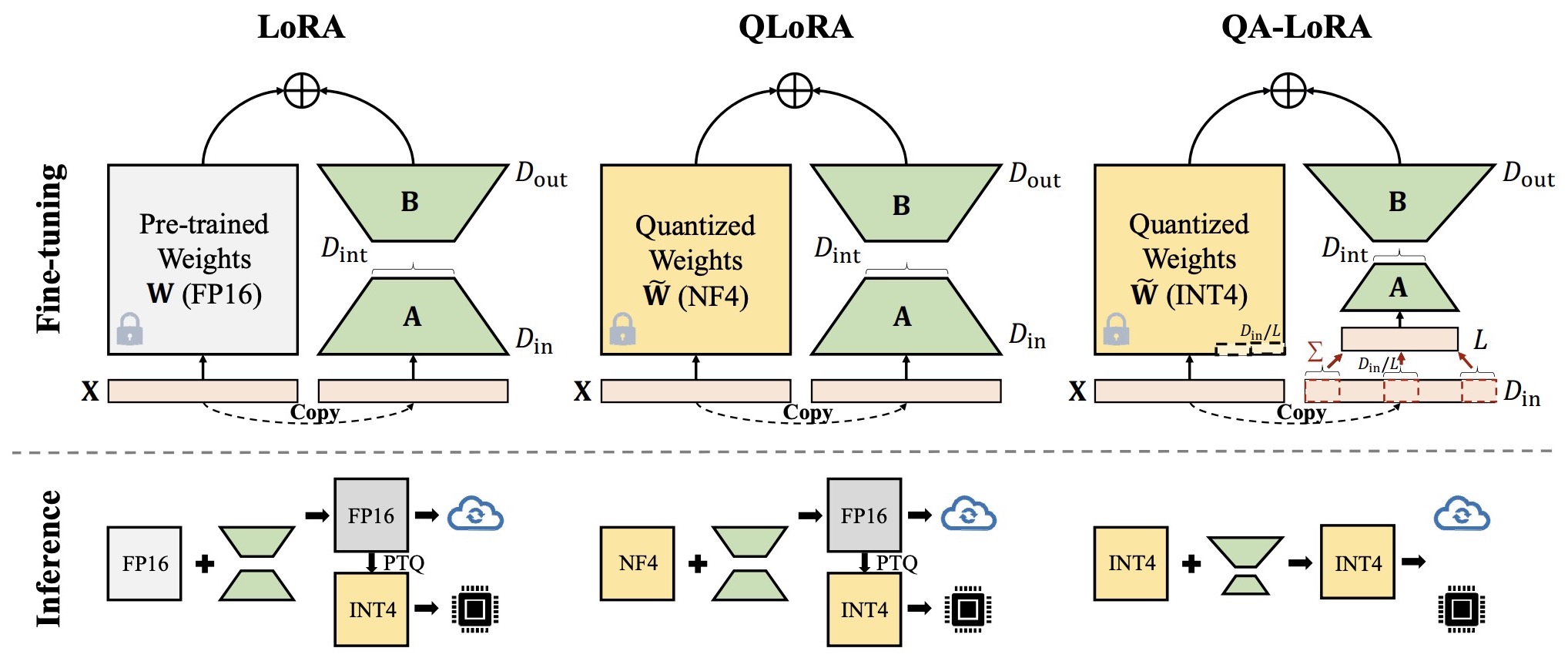
-
Fine-tuning settings:
- Datasets: Alpaca (52K) and FLAN v2 subset (320K).
- Optimizer: Paged AdamW, \(\eta = 2 \times 10^{-5}\) (LLaMA-7B/13B) or \(\eta = 1 \times 10^{-5}\) (LLaMA-33B/65B),
max_grad_norm = 0.3,batch_size = 16. - Steps: 10K (Alpaca), 20K (FLAN v2).
- Hardware: Tesla V100 GPUs (1 GPU for ≤33B models, 2 GPUs for 65B).
Algorithm steps
- Group-wise quantization of base weights into
INT4/3/2at fine-tuning start. - Group-wise LoRA pooling and adaptation — only \(L \times D_{int}\) parameters for \(A\) instead of \(D_{in} \times D_{int}\).
- Fine-tuning LoRA parameters while keeping base weights quantized.
- Merging LoRA and base weights in the quantized domain by adjusting \(\beta\) factors directly.
Advantages over prior work
- Compared to LoRA: Lower fine-tuning memory and faster inference due to quantization.
- Compared to QLoRA:
- Avoids
FP16fallback after merging. - Uses CUDA-optimized INT formats instead of
NF4, yielding >50% faster inference. - Higher accuracy at low bit widths (especially
INT2/INT3) due to quantization-aware adaptation.
- Avoids
Results
- On LLaMA and Llama 2 models, QA-LoRA matches or exceeds QLoRA’s accuracy at
INT4and significantly outperforms it atINT3andINT2. - Training time reduction: For LLaMA-13B, fine-tuning time drops from 73.1h (QLoRA) to 29.5h (QA-LoRA).
- Commonsense QA tasks show consistent improvements, with QA-LoRA (2-bit) achieving +15% accuracy over QLoRA (2-bit) with PTQ.
Comparison of LoRA, QLoRA, and QA-LoRA
- The table below summarizes key differences in methodology, quantization formats, fine-tuning characteristics, inference properties, and practical considerations for deployment for LoRA, QLoRA, and QA-LoRA.
| Aspect | LoRA (Hu et al., 2021) |
QLoRA (Dettmers et al., 2023) |
QA-LoRA (Xu et al., 2023) |
|---|---|---|---|
| Primary Goal | Parameter-efficient fine-tuning (reduce trainable parameters while preserving accuracy) | Combine low-bit quantization and LoRA to reduce fine-tuning memory | Joint low-bit quantization and LoRA with mergeability in quantized form for both fine-tuning and inference |
| Base Weight Precision During Fine-Tuning | FP16 or FP32 |
NF4 (NormalFloat4, 4-bit floating point) |
INT4, INT3, or INT2 (integer quantization) with group-wise scaling |
| LoRA Weight Precision During Fine-Tuning | FP16/FP32 |
FP16 |
Same precision as base weight (INT4/3/2) due to quantization-aware adaptation |
| Adaptation Method | Low-rank matrices A and B added to frozen base weights | Same as LoRA but applied to NF4-quantized base weights | Group-wise LoRA (shared parameters within quantization groups) for mergeability in low-bit domain |
| Quantization Granularity | N/A | Column-wise NF4 quantization of base weights |
Group-wise integer quantization (e.g., group size 32) with group-specific scale and zero |
| Post-Fine-Tuning Merge Result | Full-precision model (merging A and B into W yields FP16/FP32) |
Full-precision model (merging requires FP16 fallback) unless PTQ is applied (accuracy loss at low bits) |
Fully quantized merged model, no need for PTQ, no accuracy loss compared to full precision |
| Inference Precision | FP16/FP32 |
FP16 (without PTQ) or INT4 (with PTQ, accuracy drop) |
INT4/3/2, same as during training |
| Hardware Efficiency | Reduced training memory vs. full fine-tuning; no change in inference speed | Reduced training memory; inference slower without PTQ due to FP16 fallback; NF4 has no widespread hardware acceleration |
Reduced training memory; inference fast due to native integer kernels; compatible with existing INT quantization acceleration |
| Accuracy at Low Bit Widths | High (since no quantization) | Good at 4-bit NF4, but drops significantly with INT4 PTQ, and worse at 3-bit/2-bit |
Matches QLoRA at 4-bit NF4; outperforms significantly at INT3 and INT2 |
| Implementation Complexity | Moderate; widely supported in libraries | Moderate; requires NF4 quantization and mixed precision handling | Low; a few extra lines on top of LoRA, uses standard INT formats and group pooling |
| Representative Use Cases | PEFT when quantization is not needed or when deployment can afford FP16 |
Fine-tuning large models under memory constraints, where deployment can use FP16 or 4-bit NF4 |
Fine-tuning and deploying large models directly in INT4/3/2 on resource-limited hardware |
Refined Low-Rank Adaptation (ReLoRA)
- Proposed in Stack More Layers Differently: High-Rank Training Through Low-Rank Updates by Lialin et al. from UMass Lowell.
- Refined Low-Rank Adaptation (ReLoRA) is a low-rank training technique as an alternative approach to training large neural networks. ReLoRA utilizes low-rank updates to train high-rank networks. Put simply, they explore whether LoRA can be used for pretraining (as opposed to finetuning) LLMs in a parameter-efficient manner.
- They apply ReLoRA to pre-training transformer LLMs with up to 350M parameters and demonstrate comparable performance to regular neural network training.
- Furthermore, they observe that the efficiency of ReLoRA increases with model size, making it a promising approach for training multi-billion-parameter networks efficiently. Their findings shed light on the potential of low-rank training techniques and their implications for scaling laws.
- A caveat worth mentioning is that the researchers only pretrained models up to 350 M parameters for now (the smallest Llama 2 model is 7B parameters, for comparison).
- The following figure (source) presents an overview of their results:
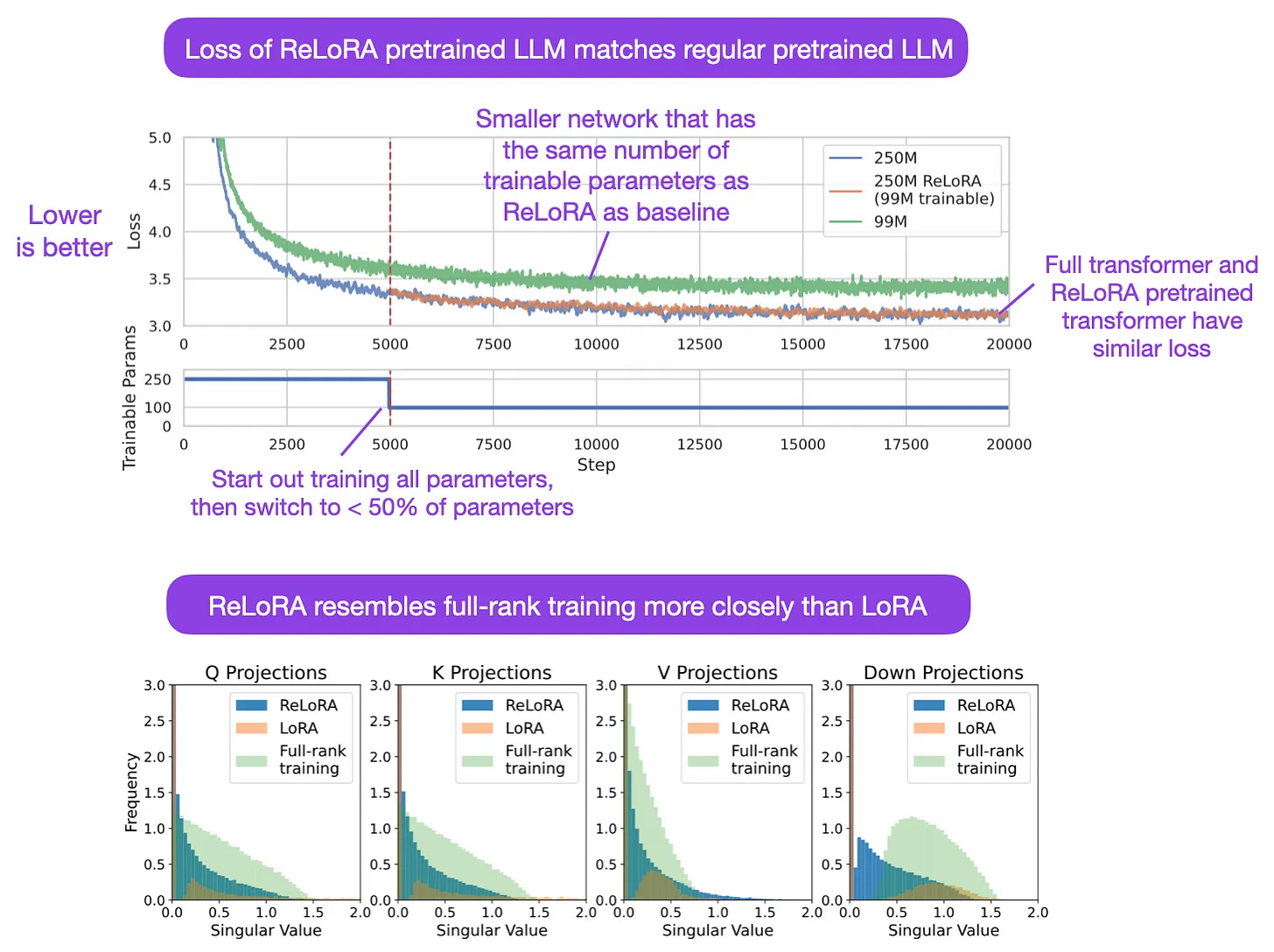
S-LoRA: Serving Thousands of Concurrent LoRA Adapters
- This paper by Sheng et al. from UC Berkeley, Stanford, and Shanghai Jiao Tong focuses on the scalable serving of LoRA (Low-Rank Adaptation) adapters for large LLMs (LLMs).
- The “pretrain-then-finetune” paradigm, widely adopted in deploying LLMs, leads to numerous fine-tuned variants, presenting significant opportunities for batched inference during serving. The paper introduces S-LoRA, a system designed for this purpose.
- S-LoRA addresses memory management challenges by storing all adapters in main memory and fetching them to GPU memory as needed. The system employs Unified Paging, a unified memory pool managing dynamic adapter weights and KV cache tensors, to reduce memory fragmentation and I/O overhead.
- The paper presents a novel tensor parallelism strategy and customized CUDA kernels for efficient heterogeneous batching of LoRA computations, enabling the serving of thousands of adapters on a single or multiple GPUs with minimal overhead.
- The following image from the paper shows separated batched computation for the base model and LoRA computation. The batched computation of the base model is implemented by GEMM. The batched computation for LoRA adapters is implemented by custom CUDA kernels which support batching various sequence lengths and adapter ranks.
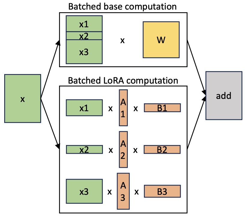
- The following image from the paper shows an overview of memory allocation in S-LoRA. S-LoRA stores all adapters in the main memory and fetches the active adapters for the current batch to the GPU memory. The GPU memory is used to store the KV cache, adapter weights, base model weights, and other temporary tensors.
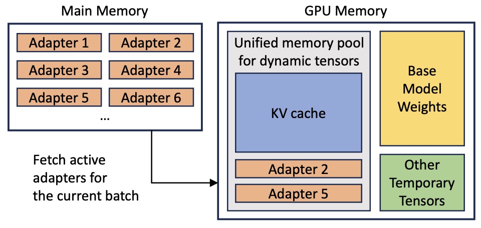
- S-LoRA’s performance is evaluated against state-of-the-art libraries like Weights PEFT and vLLM, showing up to 4 times higher throughput and the capability to serve significantly more adapters.
- The system is effective in reducing the training and communication costs in Federated Learning, making it a promising approach for deploying large LLMs in resource-constrained environments.
- This paper contributes significantly to the field of machine learning by presenting a novel and efficient method for serving a large number of LoRA adapters, a crucial aspect in the deployment of large-scale LLMs.
- Code
Predibase
- Similar to S-LoRA, Predibase, a startup, offers a unique serving infrastructure – LoRAX – which lets you cost-effectively serve many fine-tuned adapters on a single GPU in dedicated deployments.
Weight-Decomposed Low-Rank Adaptation (DoRA)
- Proposed in DoRA: Weight-Decomposed Low-Rank Adaptation by Liu et al. from NVIDIA and HKUST.
- Weight-Decomposed Low-Rank Adaptation (DoRA) is a novel Parameter-Efficient Fine-Tuning (PEFT) method that surpasses existing techniques like LoRA by decomposing pre-trained weights into magnitude and directional components for efficient fine-tuning. This method is designed to bridge the accuracy gap between LoRA-based methods and full fine-tuning, without increasing inference costs.
- The authors’ weight decomposition analysis reveals fundamental differences between full fine-tuning and LoRA, showing that directional updates play a crucial role in learning capability. DoRA employs LoRA for directional updates and introduces trainable magnitude components, enhancing learning capacity and stability.
- DoRA demonstrates superior performance across a range of tasks, including commonsense reasoning, visual instruction tuning, and image/video-text understanding, across models like LLaMA, LLaVA, and VL-BART. It achieves this by effectively managing the trade-off between the number of trainable parameters and learning capacity, without adding inference overhead.
- The following figure from the paper illustrates an overview of DoRA, which decomposes the pre-trained weight into magnitude and direction components for fine-tuning, especially with LoRA to efficiently update the direction component. Note that \(\|\cdot\|_c\) denotes the vector-wise norm of a matrix across each column vector.

- Experiments show that DoRA not only outperforms LoRA but also matches or exceeds the performance of full fine-tuning across different tasks, with significant improvements in commonsense reasoning tasks and multimodal understanding, illustrating its effectiveness and efficiency.
- The paper also explores DoRA’s compatibility with other LoRA variants, such as VeRA, and demonstrates its adaptability across different training sizes and rank settings, further establishing its utility as a versatile and powerful fine-tuning method.
- Blog
Summary of LoRA Techniques
- The following section is inspired from Cameron Woulfe’s (source) post.
- Here’s an overview of some prevalent variants of LoRA techniques:
- LoRA models the update derived for a model’s weights during finetuning with a low rank decomposition, implemented in practice as a pair of linear projections. LoRA leaves the pretrained layers of the LLM fixed and injects a trainable rank decomposition matrix into each layer of the model.
- QLoRA is (arguably) the most popular LoRA variant and uses model quantization techniques to reduce memory usage during finetuning while maintaining (roughly) equal levels of performance. QLoRA uses 4-bit quantization on the pretrained model weights and trains LoRA modules on top of this. In practice, QLoRA saves memory at the cost of slightly-reduced training speed.
- QA-LoRA is an extension of LoRA/QLoRA that further reduces the computational burden of training and deploying LLMs. It does this by combining parameter-efficient finetuning with quantization (i.e., group-wise quantization applied during training/inference).
- LoftQ studies a similar idea to QA-LoRA – applying quantization and LoRA finetuning on a pretrained model simultaneously.
- LongLoRA attempts to cheaply adapt LLMs to longer context lengths using a parameter-efficient (LoRA-based) finetuning scheme. In particular, we start with a pretrained model and finetune it to have a longer context length. This finetuning is made efficient by:
- Using sparse local attention instead of dense global attention (optional at inference time).
- Using LoRA (authors find that this works well for context extension).
- S-LoRA aims to solve the problem of deploying multiple LoRA modules that are used to adapt the same pretrained model to a variety of different tasks. Put simply, S-LoRA does the following to serve thousands of LoRA modules on a single GPU (or across GPUs):
- Stores all LoRA modules in main memory.
- Puts modules being used to run the current query into GPU memory.
- Uses unified paging to allocate GPU memory and avoid fragmentation.
- Proposes a new tensor parallelism strategy to batch LoRA computations.
- **ReLoRA refines neural network training by iteratively applying low-rank updates to achieve high-rank performance, streamlining the process for large models.
- DoRA surpasses existing techniques like LoRA by decomposing pre-trained weights into magnitude and directional components for efficient fine-tuning. This method is designed to bridge the accuracy gap between LoRA-based methods and full fine-tuning, without increasing inference costs. It employs LoRA for directional updates and introduces trainable magnitude components, enhancing learning capacity and stability.
- Many other LoRA variants exist as well:
- LQ-LoRA: uses a more sophisticated quantization scheme within QLoRA that performs better and can be adapted to a target memory budget.
- MultiLoRA: extension of LoRA that better handles complex multi-task learning scenarios.
- LoRA-FA: freezes half of the low-rank decomposition matrix (i.e., the A matrix within the product AB) to further reduce memory overhead.
- Tied-LoRA: leverages weight tying to further improve the parameter efficiency of LoRA.
- GLoRA: extends LoRA to adapt pretrained model weights and activations to each task in addition to an adapter for each layer.
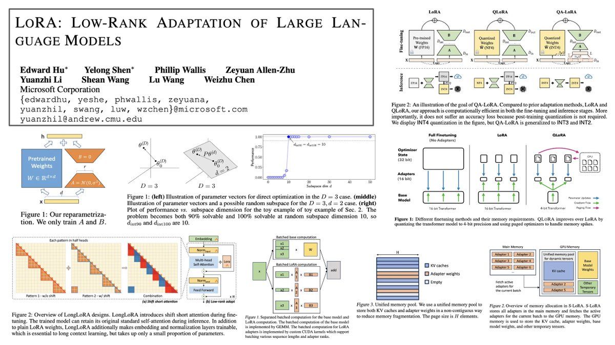
Low-rank Linear Subspace ReFT (LoReFT)
- Proposed in ReFT: Representation Finetuning for LLMs by Wu et al. from Stanford and the Pr(Ai)2R Group.
- Representation Finetuning (ReFT) is a suite of methods to modify the hidden representations of LLMs (LMs) for task-specific adaptation. Unlike traditional parameter-efficient finetuning (PEFT) methods that adapt by modifying weights, ReFT manipulates a small fraction of model representations, enhancing the interpretability and flexibility of the interventions.
- A key variant within ReFT, named Low-rank Linear Subspace ReFT (LoReFT), leverages a low-rank projection matrix to edit representations in a linear subspace. This approach is demonstrated to be 10\(\times\)–50\(\times\) more parameter-efficient compared to existing state-of-the-art PEFTs like LoRA.
- The ReFT methodology, specifically Low-rank Linear Subspace ReFT (LoReFT), operates by editing hidden representations in a linear subspace. LoReFT modifies these representations using a projection matrix \(R\), which redefines them in a low-dimensional subspace for efficiency. The matrix \(R\) has orthonormal rows, which are crucial for maintaining the quality of the intervention without adding much complexity.
- The core intervention of LoReFT, as per the distributed interchange intervention (DII) formula \(DII(b, s, R) = b + R^\top(Rs - Rb)\), leverages the projection matrix to adjust the hidden states \(b\) towards a target state \(s\) by the application of \(R\). This intervention is designed to manipulate the model output towards desired behaviors or answers subtly and effectively.
- LoReFT employs a linear transformation defined by the parameters \(W\) and \(b\) (not to be confused with the bias term), which projects the representation into the subspace before it is edited. This transformation helps in aligning the representation more closely with the task-specific features that are crucial for performance.
- Practically, LoReFT is implemented as a set of non-overlapping interventions across multiple layers of a Transformer-based model. These interventions are strategically placed to modify the behavior of the model without extensive retraining of the underlying parameters.
- Each intervention is applied after the computation of layer \(L\) representations, meaning it directly affects the computation of subsequent layers \(L+1\) to \(L+m\). This placement ensures that the interventions have a cascading effect, enhancing their impact on the final model output.
- The hyperparameter tuning for LoReFT focuses on the number and placement of interventions across the layers, optimizing both the effectiveness of each intervention and the overall computational overhead. This involves selecting the appropriate number of prefix and suffix positions in the input where interventions are most beneficial, as well as deciding on the layers where these modifications will have the most impact.
- The figure below from the paper shows an illustration of ReFT. (1) The left panel depicts an intervention I: the intervention function \(\Phi\) is applied to hidden representations at positions \(P\) in layer \(L\). (2) The right panel depicts the hyperparameters we tune when experimenting with LoReFT. Specifically, the figure depicts application of LoReFT at all layers with prefix length \(p\) = 2 and suffix length \(s\) = 2. When not tying layer weights, we train separate intervention parameters at each position and layer, resulting in 16 interventions with unique parameters in this example.
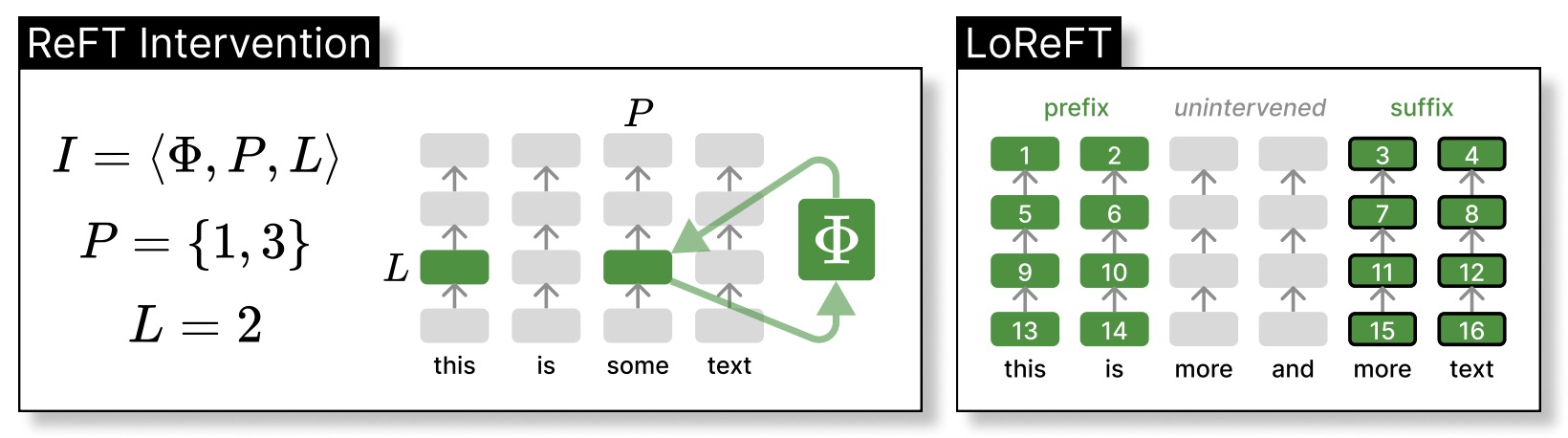
- The authors evaluate LoReFT across multiple domains, including commonsense reasoning, arithmetic reasoning, instruction-following, and natural language understanding. It is shown that LoReFT achieves competitive or superior performance on all tasks, especially shining in commonsense reasoning benchmarks.
- Implementation details reveal that LoReFT interventions are applied at selected layers and positions within the LM, optimizing both the number of interventions and their locations through hyperparameter tuning. This targeted approach allows for minimal additional computational overhead at inference.
- LoReFT is implemented in a publicly available Python library,
pyreft, which facilitates the adoption of ReFT methods by providing tools to apply these interventions on any pretrained LM from the HuggingFace model hub. - The paper establishes the potential of representation-focused finetuning as a more effective alternative to weight-based methods, setting new standards for efficiency and performance in adapting large-scale LMs to diverse tasks.
Stratified Progressive Adaptation Fine-tuning (SPAFIT)
- Proposed in SPAFIT: Stratified Progressive Adaptation Fine-tuning for Pre-trained Large LLMs by Arora and Wang from Simon Fraser University, Stratified Progressive Adaptation Fine-tuning (SPAFIT) is a novel Parameter-Efficient Fine-Tuning (PEFT) method aimed at optimizing the fine-tuning process of Transformer-based large LLMs by localizing the fine-tuning to specific layers according to their linguistic knowledge importance. This addresses issues like catastrophic forgetting and computational inefficiency common in full fine-tuning methods.
- SPAFIT organizes the model into three groups of layers, with increasing complexity of fine-tuning allowed as the layers progress from basic linguistic processing to more task-specific functions. Group 1 layers remain completely frozen, Group 2 layers undergo fine-tuning only on bias terms, and Group 3 layers are fine-tuned using both BitFit for simple parameters and Low-Rank Adaptation (LoRA) for more significant weight matrices.
- The authors conducted experiments using the BERT-large-cased model across nine tasks from the GLUE benchmark. Their results demonstrate that SPAFIT can achieve or exceed the performance of full fine-tuning and other PEFT methods like Full BitFit and Full LoRA while fine-tuning significantly fewer parameters.
- The figure below from the paper illustrates an example implementation of SPAFIT on BERT.

- Notable results include SPAFIT models achieving the best performance on tasks involving sentence similarity, like MRPC and STS-B, and showing a substantial reduction in the number of parameters fine-tuned—highlighting SPAFIT’s efficiency.
- The research suggests that different types of linguistic knowledge can indeed be localized to specific layers of an LLM, potentially leading to more targeted and efficient fine-tuning strategies.
- The paper raises points for future investigation, including the application of SPAFIT to more complex tasks like summarization and to models that contain both encoder and decoder architectures. The study also acknowledges the need for further analysis on the optimal balance of parameter efficiency against task performance and the extent of adaptation necessary at different layers.
BitFit
- Proposed in BitFit: Simple Parameter-efficient Fine-tuning for Transformer-based Masked Language-models by Ben-Zaken et al. from Yoav Goldberg’s group at Bar Ilan University and the Allen Institute for Artificial Intelligence introduces BitFit, a fine-tuning method for pre-trained BERT models. BitFit focuses on updating only the bias-terms of the model, which are a minimal fraction of the model’s parameters, effectively reducing the memory footprint and computational demands typically associated with full model fine-tuning.
- BitFit’s methodology leverages the observation that fine-tuning often doesn’t require extensive retraining of all parameters. Instead, fine-tuning only the bias terms achieves competitive results compared to full model fine-tuning, especially with small to medium-sized datasets. In scenarios permitting slight performance degradation, the method can be constrained to adjust only two specific types of bias terms, representing just 0.04% of the total model parameters.
- Implementation details include freezing the transformer-encoder’s main weights and training only the bias terms along with a task-specific classification layer. This approach allows the model to handle multiple tasks efficiently in a streaming fashion without requiring simultaneous access to all task datasets.
- Experimental results on the GLUE benchmark show that BitFit is comparable or superior to full fine-tuning in several NLP tasks. It also outperforms other parameter-efficient methods like Diff-Pruning and Adapters in terms of the number of parameters modified, showcasing its effectiveness in achieving high performance with significantly fewer trainable parameters.
- The findings underscore the potential of focusing fine-tuning efforts on a small subset of parameters, specifically bias terms, to maintain or even enhance performance while minimizing computational costs. This approach also prompts further exploration of the role of bias terms in neural networks and their impact on model behavior and task transferability.
NOLA
- Proposed in NOLA: Compressing LoRA Using Linear Combination of Random Basis by Koohpayegani et al. in ICLR 2024, NOLA is a novel method for compressing large LLMs (LLMs) that addresses the limitations of Low-Rank Adaptation (LoRA). NOLA reparameterizes the rank-decomposition matrices used in LoRA through linear combinations of randomly generated basis matrices, significantly reducing the parameter count by optimizing only the mixture coefficients.
- NOLA decouples the number of trainable parameters from both the rank choice and network architecture, unlike LoRA, where parameters are inherently dependent on the matrix dimensions and rank, which must be an integer. This method not only preserves the adaptation quality but also allows for extreme compression, achieving up to 20 times fewer parameters than the most compressed LoRA models without loss of performance.
- The method’s implementation includes using a pseudo-random number generator for creating basis matrices, where the generator’s seed and the linear coefficients are stored, greatly reducing storage requirements. Quantization of these coefficients further minimizes storage needs without impacting model performance.
- The figure below from the paper shows the process that NOLA follows. After constraining the rank of \(\Delta W\) by decomposing it to \(A \times B\), we reparametrize A and B to be a linear combination of several random basis matrices. We freeze the basis and W and learn the combination coefficients. To reconstruct the model, we store the coefficients and the seed of the random generator which is a single scalar. NOLA results in more compression compared to LoRA and more importantly decouples the compression ratio from the rank and dimensions of W. One can reduce the number of parameters to 4 times smaller than rank=1 of LoRA which is not possible with LoRA due to rank being an integer number.

- Detailed experimental evaluations across several tasks and models, including GPT-2 and LLaMA-2, showcase NOLA’s effectiveness. It maintains or exceeds benchmark metrics such as BLEU and ROUGE-L while using significantly fewer parameters compared to both LoRA and full model fine-tuning.
- The approach’s versatility is demonstrated through its application not only in natural language processing tasks but also in adapting Vision Transformer (ViT) models for image classification, indicating its potential widespread applicability across different types of deep learning architectures.
- Code
Matrix of Rank Adaptation (MoRA)
- Proposed in MoRA: High-Rank Updating for Parameter-Efficient Fine-Tuning by Jiang et al. from Beihang University and Microsoft introduces a novel method, MoRA (Matrix of Rank Adaptation) is a parameter-efficient fine-tuning (PEFT) technique for LLMs. The authors identify limitations in existing PEFT methods, particularly Low-Rank Adaptation (LoRA), which may restrict LLMs’ ability to learn and retain new knowledge. To address these issues, MoRA employs a high-rank updating mechanism using a square matrix to achieve greater flexibility and effectiveness without increasing the number of trainable parameters.
- MoRA utilizes non-parameterized operators to adjust input and output dimensions, ensuring the weight can be integrated back into LLMs like LoRA. The method involves the following steps:
- Reduction of Input Dimension: Non-parameter operators reduce the input dimension for the square matrix.
- Increase of Output Dimension: Corresponding operators increase the output dimension, maintaining the number of trainable parameters while achieving high-rank updates.
- The figure below from the paper illustrates an overview of our method compared to LoRA under same number of trainable parameters. \(W\) is the frozen weight from model. \(A\) and \(B\) are trainable low-rank matrices in LoRA. \(M\) is the trainable matrix in our method. Gray parts are non-parameter operators to reducing the input dimension and increasing the output dimension. \(r\) represents the rank in two methods.
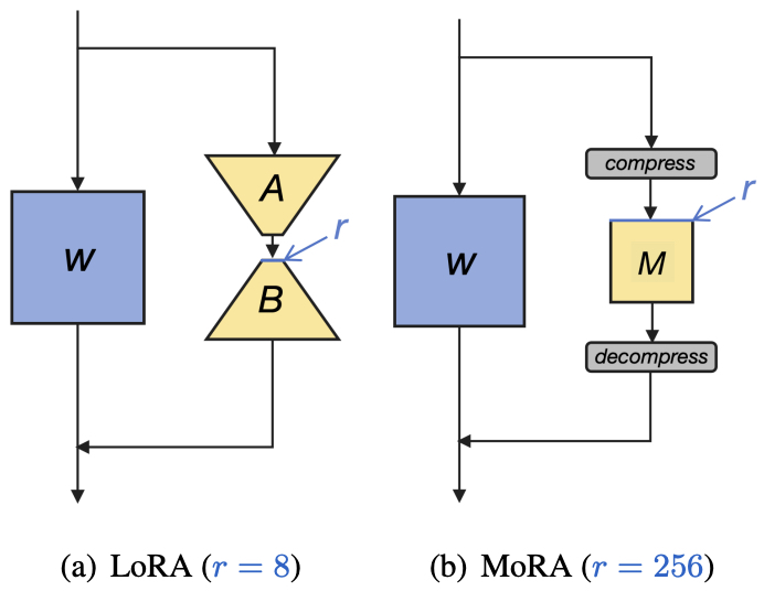
- The authors comprehensively evaluate MoRA across five tasks—instruction tuning, mathematical reasoning, continual pretraining, memory, and pretraining—demonstrating that MoRA outperforms LoRA in memory-intensive tasks and achieves comparable performance in other areas.
- Technical Details and Implementation:
- Low-Rank Limitation in LoRA: LoRA uses low-rank matrices to approximate full-rank updates, limiting its capacity to store new information, especially in memory-intensive tasks. The low-rank matrices A and B in LoRA struggle to fully capture the complexity needed for tasks requiring substantial knowledge enhancement.
- High-Rank Updating in MoRA: MoRA replaces the low-rank matrices with a square matrix, significantly increasing the rank and thus the capacity for updates. For example, LoRA with rank 8 employs matrices \(A \in \mathbb{R}^{4096 \times 8}\) and \(B \in \mathbb{R}^{8 \times 4096}\), while MoRA uses a square matrix \(M \in \mathbb{R}^{256 \times 256}\), achieving a higher rank with the same number of parameters.
- Compression and Decompression Functions: MoRA employs various methods to implement compression and decompression functions, including truncation, sharing rows/columns, reshaping, and rotation. These methods help reduce the input dimension and increase the output dimension effectively.
- Rotation Operators: Inspired by RoPE (Rotary Position Embedding), MoRA introduces rotation operators to differentiate inputs, enhancing the expressiveness of the square matrix.
- Evaluation and Results:
- Memory Task: In memorizing UUID pairs, MoRA showed significant improvements over LoRA with the same number of trainable parameters. MoRA required fewer training steps to achieve high accuracy compared to LoRA, demonstrating its effectiveness in memory-intensive tasks.
- Fine-Tuning Tasks: MoRA was evaluated on instruction tuning (using Tülu v2 dataset), mathematical reasoning (using MetaMath, GSM8K, MATH), and continual pretraining (in biomedical and financial domains). It matched LoRA’s performance in instruction tuning and mathematical reasoning but outperformed LoRA in continual pretraining tasks, benefiting from high-rank updating.
- Pretraining: MoRA and a variant, ReMoRA (which merges updates back into the model during training), were evaluated on pretraining transformers from scratch on the C4 dataset. MoRA showed better pretraining loss and perplexity metrics compared to LoRA and ReLoRA, further validating the advantages of high-rank updating.
- MoRA addresses the limitations of low-rank updates in LoRA by employing high-rank matrices, significantly enhancing the model’s capacity to learn and memorize new knowledge. This method shows promise for improving parameter-efficient fine-tuning of LLMs, especially in memory-intensive and domain-specific tasks. The authors provide comprehensive implementation details and empirical evaluations, establishing MoRA as an effective advancement in the field of PEFT.
Which PEFT Technique to Choose: A Mental Model
- Choosing a PEFT involves simply matching them with your objectives as shown in the figure below.
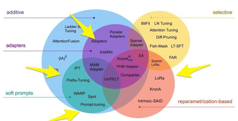
Soft Prompt Tuning
-
What: Soft Prompt tuning involves adding a small trainable prefix to the input of the pre-trained LLM during fine-tuning, which modifies the representation learned by the pre-trained model to better suit the downstream task.
-
When to use: Prompt Tuning is a good choice when you have a large pre-trained LLM but want to fine-tune it for multiple different downstream tasks at inference time with minimal computational resources. It is also useful when you want to generate diverse and high-quality text outputs based on specific prompts.
Prefix Tuning
-
What: Prefix Tuning involves learning a set of trainable parameters that modify the pre-trained LLM’s hidden states in response to task-specific prompts during inference, effectively fine-tuning the model at inference time.
-
When to use: When you want to fine-tune a pre-trained LLM for a specific downstream task and have limited computational resources when you want to modify the representation learned by the pre-trained model for a particular task.
Adapters
-
What: Adapters are tiny modules that are added to pre-trained LLMs, typically between the pre-trained layers, to adapt the model to new downstream tasks. During fine-tuning, only the weights of the adapter are learned, while the pre-trained model’s parameters remain fixed.
-
When to use: When you need to fine-tune multiple downstream tasks on the same pre-trained model. Additionally, Adapters are flexible and can be quickly and easily plugged into different parts of the pre-trained model without requiring major modifications.
BitFit
-
What: BitFit simplifies the fine-tuning process by only updating the bias terms of the model, reducing the number of parameters that need to be modified.
-
When to use: BitFit is an excellent choice when computational resources are a constraint or when working with smaller datasets. It’s especially suited for tasks where slight performance compromises are acceptable in exchange for greater efficiency.
- Key Features:
- Bias-Only Training: By focusing on updating only the bias terms, BitFit significantly lowers the computational demands and memory usage.
- Efficient Adaptability: This method achieves comparable results to more extensive fine-tuning methods with far fewer parameter updates, making it ideal for rapid deployment and iterative development.
- Process:
- Freezing Main Weights: The main weights of the Transformer encoder are frozen, preserving the pre-trained knowledge.
- Bias Term Training: Only the bias terms are fine-tuned along with a task-specific classification layer, providing an efficient way to adapt the model to new tasks.
- Evaluation Across Tasks: BitFit’s efficacy is tested on various NLP tasks, showing its capability to maintain high performance with minimal parameter adjustments.
LoRA
-
What: LoRA (Low-Rank Adaptation) is a technique that modifies the pre-trained LLM’s attention mechanism during fine-tuning by introducing a low-rank matrix factorization that learns task-specific attention patterns.
-
When to use: LoRA is a good choice when you want to fine-tune a pre-trained LLM for a specific downstream task that requires task-specific attention patterns. It is also useful when you have limited computational resources and want to reduce the number of trainable parameters in the model. Specifically:
- Memory Efficiency is Desired but Not Critical: LoRA offers substantial savings in terms of parameters and computational requirements. If you’re looking to achieve a balanced reduction in trainable parameters without diving into the complexities of quantization, LoRA is an ideal choice.
- Real-time Application: LoRA ensures no added inference latency, making it suitable for real-time applications.
- Task-Switching is Required: LoRA can share the pretrained model across multiple tasks, reducing the need for maintaining separate models for each task.
QLoRA
-
What: QLoRA (Quantized Low-Rank Adaptation) is an advanced fine-tuning technique that integrates quantization with low-rank adaptation, allowing for efficient fine-tuning of large LLMs with significantly reduced memory usage.
-
When to use: QLoRA is ideal for scenarios where memory and computational efficiency are paramount, particularly when fine-tuning very large models on limited hardware. It is especially useful when working with low-bit model environments or when full 16-bit fine-tuning would be prohibitively expensive.
- Key Features:
- 4-bit Quantization: QLoRA uses a novel 4-bit NormalFloat (
NF4) quantization, optimized for normally distributed weights, to reduce the memory footprint. - Double Quantization: This technique further reduces memory usage by quantizing the quantization constants.
- Paged Optimizers: These manage memory spikes during gradient checkpointing, enabling stable fine-tuning on a single GPU.
- 4-bit Quantization: QLoRA uses a novel 4-bit NormalFloat (
- Process:
- Model Quantization: The pre-trained model is quantized to 4-bit precision using
NF4. - Adding LoRA Weights: LoRA weights are integrated into the quantized model.
- Fine-Tuning: The LoRA weights are fine-tuned, with gradients backpropagated through the frozen quantized model.
- Double Quantization: Quantization constants are further quantized to minimize memory usage.
- Model Quantization: The pre-trained model is quantized to 4-bit precision using
- Key Features:
QA-LoRA
-
What: QA-LoRA is a specialized technique for fine-tuning low-bit diffusion models. It integrates quantization-aware strategies with Low-Rank Adaptation (LoRA) principles, providing an efficient way to handle low-bit model environments.
-
When to use: Ideal for scenarios where the primary goal is to optimize memory usage and computational efficiency in low-bit settings. This method is particularly effective when traditional fine-tuning approaches fall short due to the constraints of low-bit environments.
- Key Features:
- Quantization-Aware Approach: QA-LoRA uniquely combines LoRA weights with full-precision model weights, then jointly quantizes them, enhancing memory and computational efficiency during inference.
- Efficient for Low-Bit Models: Tailored for low-bit diffusion models, it addresses the specific challenges posed by these environments, making it a standout choice in such contexts.
- Process:
- Adding LoRA Weights: QA-LoRA begins by integrating LoRA weights into the pre-trained model.
- Fine-Tuning LoRA Weights: These weights are then fine-tuned, focusing solely on the LoRA weights while keeping the original model weights unchanged.
- Merging Weights: Post-fine-tuning, the LoRA and original model weights are merged.
- Quantization: The merged weights undergo quantization to a lower-bit format, crucial for reducing memory and computational costs.
ReLoRA
-
What: ReLoRA is an innovative approach for training high-rank networks efficiently. It revises the Low-Rank Adaptation method by iteratively applying low-rank updates to gradually increase the model’s effective rank.
-
When to use: Best suited for training large-scale models, particularly when the objective is to achieve high-rank training outcomes with less computational expenditure. ReLoRA is especially valuable for large transformer LLMs where resource efficiency is critical.
- Key Features:
- Iterative Low-Rank Updates: Unlike traditional low-rank methods, ReLoRA applies updates in an iterative manner, each time incrementally enhancing the model’s rank, leading to more efficient high-rank network training.
- Resource Efficiency: Allows for training of large, high-performing models while significantly reducing computational demands.
- Differentiation from Other Techniques:
- ReLoRA stands out from previous techniques like standard LoRA by its unique iterative process. This method incrementally increases the rank of the model through successive low-rank updates, enabling more dynamic and refined training for large-scale models.
S-LoRA
-
What: S-LoRA is a scalable system for serving multiple LoRA (Low-Rank Adaptation) adapters concurrently in large LLMs (LLMs). It manages memory efficiently by storing all adapters in main memory and dynamically fetching them to GPU memory. The system uses customized CUDA kernels for batch processing, optimizing both memory usage and computational efficiency.
-
When to use: S-LoRA is ideal for scenarios where many fine-tuned variants of LLMs need to be served simultaneously with high throughput. It significantly reduces memory fragmentation and I/O overhead, making it suitable for large-scale deployments in resource-constrained environments.
- Key Features:
- Efficient Memory Management: Utilizes a unified memory pool to manage adapter weights dynamically, reducing memory fragmentation.
- High Throughput Serving: Custom CUDA kernels enable efficient heterogeneous batching of LoRA computations, allowing the serving of thousands of adapters with minimal overhead.
- Reduced Training and Communication Costs: Offers an effective solution in federated learning scenarios by lowering the costs associated with training and data communication.
- Process:
- Storage of Adapters: All adapters are stored in the main memory, ready for dynamic retrieval.
- Dynamic Fetching: Adapters required for current computations are fetched into GPU memory as needed.
- Batch Processing: Customized CUDA kernels facilitate batch processing, ensuring efficient computation across various sequence lengths and adapter ranks.
DoRA
-
What: DoRA is an advanced fine-tuning method that decomposes pre-trained model weights into magnitude and directional components. This decomposition facilitates efficient fine-tuning by employing LoRA for directional updates and introducing trainable magnitude components to enhance the learning capacity and stability.
-
When to use: DoRA is particularly effective when there is a need to bridge the performance gap between LoRA-based methods and full fine-tuning without increasing inference costs. It’s suitable for tasks that require high performance, such as commonsense reasoning, visual instruction tuning, and multimodal understanding.
- Key Features:
- Weight Decomposition: Separates weights into magnitude and direction, allowing for targeted updates that enhance learning capability without additional inference overhead.
- Enhanced Learning Capacity: Integrates trainable magnitude components with directional updates, providing a balanced approach to fine-tuning that improves both stability and learning capacity.
- Versatility Across Tasks: Demonstrates superior performance across various tasks and models, proving its adaptability and effectiveness in different settings.
- Process:
- Decomposition of Weights: Begins with the decomposition of pre-trained model weights into their magnitude and directional components.
- Directional Updates Using LoRA: Employs LoRA specifically for updating directional components during fine-tuning.
- Training of Magnitude Components: Trainable magnitude components are fine-tuned separately, enhancing the overall learning capacity of the model.
- Performance Evaluation: The effectiveness of DoRA is validated across multiple tasks, showcasing significant performance improvements compared to other fine-tuning methods.
SPAFIT
-
What: SPAFIT (Stratified Progressive Adaptation Fine-tuning) is a Parameter-Efficient Fine-Tuning (PEFT) method that targets specific layers of a Transformer-based large language model according to their contribution to linguistic knowledge.
-
When to use: SPAFIT is effective when you want to avoid the pitfalls of catastrophic forgetting and computational inefficiency typical in full model fine-tuning. It’s particularly useful for tasks that require different levels of linguistic processing, allowing for tailored adaptation.
- Key Features:
- Layer-Specific Fine-Tuning: SPAFIT divides the model into three groups, allowing each group of layers to be fine-tuned to varying extents based on their importance to task performance.
- Efficiency and Performance: By fine-tuning fewer parameters, SPAFIT achieves competitive or superior results compared to full fine-tuning, particularly on tasks involving sentence similarity.
- Process:
- Layer Grouping: Model layers are categorized into three groups based on their function and linguistic contribution.
- Adaptive Fine-Tuning: Group 1 layers remain frozen, Group 2 layers are fine-tuned only on bias terms, and Group 3 layers undergo a more comprehensive fine-tuning using BitFit and LoRA for different components.
- Performance Evaluation: SPAFIT’s effectiveness is validated across multiple NLP tasks, showing strong results with fewer fine-tuned parameters.
NOLA
-
What: NOLA is a novel method for compressing large LLMs that reparameterizes the matrices used in Low-Rank Adaptation (LoRA) through linear combinations of randomly generated basis matrices, drastically reducing the parameter count.
-
When to use: Ideal for situations where extreme model compression is necessary without sacrificing performance, making it suitable for deployment in resource-constrained environments or when model storage costs need to be minimized.
- Key Features:
- Parameter Compression: Achieves up to 20 times fewer parameters than the most compressed LoRA models.
- Decoupling Parameter Count: Separates the number of trainable parameters from the rank choice and network architecture, allowing for more flexible and efficient model compression.
- Process:
- Matrix Reparameterization: Decomposes weight changes into two matrices, \(A\) and \(B\), which are then reparameterized using a linear combination of random basis matrices.
- Learning Combination Coefficients: Focuses on optimizing the mixture coefficients for these basis matrices while keeping the original matrices frozen.
- Storage Optimization: Stores only the coefficients and the seed of the random number generator used for creating the basis matrices, significantly reducing storage requirements.
- Evaluation on Multiple Tasks: Demonstrates effectiveness across various tasks and models, maintaining or exceeding benchmark metrics while significantly reducing the parameter count.
MoRA
-
What: MoRA (Matrix of Rank Adaptation) is an advanced fine-tuning technique designed to enhance the capacity of large LLMs (LLMs) to learn and retain new knowledge. It replaces the low-rank matrices used in LoRA with a high-rank square matrix, significantly increasing the model’s update capacity without increasing the number of trainable parameters. This method introduces non-parameterized operators to adjust the input and output dimensions, ensuring efficient integration with existing LLMs.
- When to use: MoRA is particularly effective for tasks that require substantial knowledge enhancement and memory capacity. It is well-suited for scenarios where:
- Memory-Intensive Tasks: The task demands significant memorization and the retention of new knowledge, such as continual pretraining and memory tasks.
- Limited Resources: You need to maximize performance while maintaining low computational and memory overheads.
- Performance Matching or Exceeding LoRA: The method outperforms LoRA on memory-intensive tasks and achieves comparable performance on other tasks, making it a versatile choice across various applications.
- Key Features:
- High-Rank Updates: Utilizes a square matrix to achieve high-rank updates, significantly increasing the model’s capacity to learn and retain new information.
- Efficient Parameter Use: Maintains the same number of trainable parameters as LoRA by employing non-parameterized operators for input and output dimension adjustments.
- Versatility Across Tasks: Demonstrates superior performance in memory-intensive tasks and matches performance in other fine-tuning scenarios, proving its effectiveness across diverse applications.
- Process:
- Input Dimension Reduction: Non-parameterized operators reduce the input dimension for the high-rank square matrix.
- Output Dimension Increase: Corresponding operators increase the output dimension, maintaining parameter efficiency.
- Integration with LLMs: The high-rank matrix and operators can be integrated back into the LLM, similar to LoRA, ensuring seamless deployment.
- Empirical Evaluation: Comprehensive evaluation across multiple tasks, including instruction tuning, mathematical reasoning, and continual pretraining, demonstrating significant improvements in memory-intensive tasks and comparable performance in others.
Comparative Analysis of Popular PEFT Methods
| PEFT Methods | Description | When to Use | Computational Overhead | Memory Efficiency | Versatility across Tasks | Performance Impact |
|---|---|---|---|---|---|---|
| Prompt Tuning | Modifies LLM's hidden states with trainable parameters in response to task-specific prompts. | Large pre-trained LLM. Adaptation to multiple tasks. |
Low | Moderate | High | Depends on prompt quality |
| Prefix Tuning | Adds a trainable prefix to modify LLM's learned representation. | Task-specific adaptation. Limited resources. |
Low | Moderate | Moderate | Can vary, but usually positive with proper tuning |
| Adapters | Inserts neural modules between LLM layers; only adapter weights are updated during fine-tuning. | Multiple tasks on one LLM. Flexibility required. |
Moderate | Good (only adapters are fine-tuned) | High (can be added for multiple tasks) | Typically positive if adapters are well-tuned |
| LoRA | Introduces a low-rank matrix into the attention mechanism to learn task-specific patterns. | Tasks with specialized attention requirements. Limited resources. |
Low-Moderate | Good | Moderate | Generally positive with good training |
| QLoRA | Builds on LoRA with quantization for enhanced memory efficiency. | Strict memory constraints. Emphasis on performance & efficiency. |
Low | Excellent | High | Comparable or better than full fine-tuning |
| QA-LoRA | Enhances LoRA with quantization-aware techniques for fine-tuning low-bit diffusion models. | Optimizing efficiency in low-bit settings. Resource-constrained environments. |
Low | Excellent | Moderate | Enhanced efficiency and effectiveness in specific settings |
| ReLoRA | Iteratively applies low-rank updates for efficient training of high-rank networks. | Large-scale models requiring high-rank training with reduced resources. | Moderate | Good | Moderate | Achieves high-rank training efficiency and performance |
| S-LoRA | System for scalable serving of LoRA adapters in LLMs, using a unified memory management system and custom CUDA kernels for batch processing. | Deploying multiple LLM variants efficiently. High throughput needs in serving. |
Moderate | Good (efficient memory management) | High (supports thousands of concurrent adapters) | Increases throughput, reduces costs in federated settings |
| DoRA | Decomposes pre-trained weights into magnitude and directional components for fine-tuning, employing LoRA for directional updates to enhance learning capacity and stability. | Improving learning capacity without adding inference overhead. High performance across diverse tasks. |
Low | Good | High (adaptable across various models and tasks) | Matches or exceeds full fine-tuning performance |
| SPAFIT | Stratifies layer fine-tuning by linguistic importance, selectively applying adaptations. | Optimal resource allocation. High performance with reduced parameter tuning. |
Low to moderate | High (fine-tunes fewer parameters) | High (effective across multiple tasks) | Matches or exceeds full model tuning |
| BitFit | Updates only bias terms of pre-trained BERT models, reducing the fine-tuning overhead. | Small to medium datasets. Minimal performance degradation acceptable. |
Low | High (minimal parameters are updated) | Moderate (depends on the importance of bias terms) | Comparable or superior to full fine-tuning |
| NOLA | Compresses LoRA using a linear combination of random basis matrices, minimizing parameter counts. | Extreme model compression without losing performance. Resource-constrained environments. |
Low | Excellent (up to 20 times fewer parameters) | High (effective across NLP and Vision tasks) | Maintains or exceeds benchmark metrics |
| MoRA | Employs a high-rank square matrix for updates, enhancing the model's capacity to learn and retain new knowledge while maintaining parameter efficiency. | Tasks requiring substantial knowledge enhancement and memory capacity. Limited resources. |
Low-Moderate | Good | High | Outperforms LoRA on memory-intensive tasks and matches performance on others |
Practical Tips for Finetuning LLMs Using LoRA
-
This section is inspired by the findings of Sebastian Raschka’s blog talking about practical tips for finetuning.
-
Consistency in LLM Training: Despite the inherent randomness in training models on GPUs, the outcomes of LoRA experiments remain consistent across multiple runs, which is promising for comparative studies.
-
QLoRA Compute-Memory Trade-offs: Quantized LoRA (QLoRA) offers a 33% reduction in GPU memory usage at the cost of a 33% increase in runtime, proving to be a viable alternative to regular LoRA when facing GPU memory constraints.
-
Learning Rate Schedulers: Using learning rate schedulers like cosine annealing can optimize convergence during training and avoid overshooting the loss minima. While it has a notable impact on SGD optimizer performance, it makes less difference when using Adam or AdamW optimizers.
-
Choice of Optimizers: The optimizer choice (Adam vs. SGD) doesn’t significantly impact the peak memory demands of LLM training, and swapping Adam for SGD may not provide substantial memory savings, especially with a small LoRA rank (r).
-
Impact of Multiple Training Epochs: Iterating multiple times over a static dataset in multi-epoch training may not be beneficial and could deteriorate model performance, possibly due to overfitting.
-
Applying LoRA Across Layers: Enabling LoRA across all layers, not just the Key and Value matrices, can significantly increase model performance, though it also increases the number of trainable parameters and memory requirements.
-
LoRA Hyperparameters: Adjusting the LoRA rank (r) and selecting an appropriate alpha value are crucial. A heuristic that yielded good results was setting alpha at twice the rank’s value, with r=256 and alpha=512 being the best setting in one particular case.
-
Fine-tuning Large Models: LoRA allows for fine-tuning 7 billion parameter LLMs on a single GPU with 14 GB of RAM within a few hours. However, optimizing an LLM to excel across all benchmark tasks may be unattainable with a static dataset.
-
-
Additionally, the article addresses common questions related to LoRA:
-
Importance of Dataset: The dataset used for fine-tuning is critical, and data quality is very important. Experiments showed that a curated dataset with fewer examples (like LIMA) could yield better performance than larger datasets (like Alpaca).
-
LoRA for Domain Adaptation: LoRA’s effectiveness for domain adaptation requires further investigation. Including task-specific examples in the fine-tuning process is recommended.
-
Selecting the Best Rank: Choosing the best rank for LoRA is a hyperparameter that needs to be explored for each LLM and dataset. A larger rank could lead to overfitting, while a smaller rank may not capture diverse tasks within a dataset.
-
Enabling LoRA for All Layers: Exploring the impact of enabling LoRA for different combinations of layers is suggested for future experiments.
-
Avoiding Overfitting: To prevent overfitting, one could decrease the rank or increase the dataset size, adjust the weight decay rate, or consider increasing the dropout value for LoRA layers.
-
Other Optimizers: Exploring other optimizers, such as Sophia, which promises faster training and better performance than Adam, is suggested for future research.
-
Factors Influencing Memory Usage: Model size, batch size, the number of trainable LoRA parameters, and dataset size can influence memory usage. Shorter training sequences can lead to substantial memory savings.
-
Related: Surgical fine-tuning
- While not exactly a PEFT method, Surgical fine-tuning by Lee et al. from Finn’s group at Stanford is a method of selectively updating specific layers in a neural network based on how a fine-tuning dataset differs from the original pretraining dataset, rather than retraining every layer.
- Motivation:
- Layer Specificity: Early layers in a neural network capture fundamental features of inputs (e.g., edges or shapes in images), while deeper layers combine these features for predictions (e.g., classifying images).
- Efficiency: Rather than universally fine-tuning every layer, selectively updating specific layers can achieve better performance, especially when the fine-tuning dataset has notable differences from the pretraining dataset.
- Approaches:
- Manual Approach:
- Fine-tune each layer individually and create a distinct model for each layer.
- Compare the performance of each model to identify the best layers for fine-tuning.
- Automated Approach:
- Calculate gradients for each layer.
- Derive relative gradients by dividing the layer’s gradient by its weight magnitude.
- Normalize these relative gradients across layers, ranking them between 0 to 1.
- Assign learning rates for layers based on their normalized relative gradient value during training.
- Based on the findings in this paper, here are some tips for determining which layers to fine-tune when adapting a pretrained model to a new target distribution:
- Consider the type of distribution shift between the source and target data:
- For input-level shifts like image corruptions, fine-tuning earlier layers (first conv block) tends to work best. This allows the model to adapt to changes in the input while preserving higher-level features.
- For feature-level shifts where the feature representations differ between source and target, fine-tuning middle layers (middle conv blocks) tends to work well. This tunes the mid-level features without distorting low-level or high-level representations.
- For output-level shifts like label distribution changes, fine-tuning later layers (fully connected classifier) tends to be most effective. This keeps the feature hierarchy intact and only adapts the output mapping.
- Try fine-tuning only a single contiguous block of layers while freezing others. Systematically test first, middle, and last blocks to find the best one.
- Use criteria like relative gradient norms to automatically identify layers that change the most for the target data. Fine-tuning those with higher relative gradients can work better than full fine-tuning.
- When in doubt, fine-tuning only the classifier head is a solid default that outperforms no fine-tuning. But for shifts related to inputs or features, surgical fine-tuning of earlier layers can improve over this default.
- If possible, do some quick validation experiments to directly compare different surgical fine-tuning choices on a small held-out set of target data.
- The key insight is that different parts of the network are best suited for adapting to different types of distribution shifts between the source and target data.
- Consider the type of distribution shift between the source and target data:
- Manual Approach:
- Results:
- CIFAR-C Dataset:
- Manual approach yielded an accuracy of 82.8%.
- Fine-tuning the entire network resulted in 79.9% accuracy.
- The automated approach achieved an accuracy of 81.4%.
- CIFAR-C Dataset:
- Significance: Surgical fine-tuning is rooted in understanding how neural networks process input. This enhanced understanding can drive the discovery of more efficient methods to improve machine learning models.
- Consideration: For more complex datasets, discerning differences between pretraining and fine-tuning datasets can be challenging. This complexity might make automated approaches like the one proposed more valuable, even if it didn’t yield the best performance on CIFAR-C.
LoRA vs. QLoRA experimentation by Sebastian Raschka
- This section is taken from Sebastian Raschka’s post on LoRA & QLoRA experiments to finetune open-source LLMs, and presents his learnings:
- Despite embracing the inherent randomness of LLM training (or when training models on GPUs in general), the outcomes remain remarkably consistent across multiple runs.
- QLoRA presents a trade-off that might be worthwhile if you’re constrained by GPU memory. It offers 33% memory savings at the cost of a 33% increase in runtime.
- When finetuning LLMs, the choice of optimizer shouldn’t be a major concern. While SGD on its own is suboptimal, there’s minimal variation in outcomes whether you employ AdamW, SGD with a scheduler, or AdamW with a scheduler.
- While Adam is often labeled a memory-intensive optimizer due to its introduction of two new parameters for every model parameter, this doesn’t significantly affect the peak memory demands of the LLM. This is because the majority of the memory is allocated for large matrix multiplications rather than retaining extra parameters.
- For static datasets, iterating multiple times as done in multi-epoch training might not be beneficial. It often deteriorates the results, probably due to overfitting.
- If you’re incorporating LoRA, ensure it’s applied across all layers, not just to the Key and Value matrices, to maximize model performance.
- Adjusting the LoRA rank is essential, and so is selecting an apt alpha value. A good heuristic is setting alpha at twice the rank’s value.
- 7B models can be finetuned efficiently within a few hours on a single GPU possessing 14 Gb of RAM.
- With a static dataset, optimizing an LLM to excel across all benchmark tasks is unattainable. Addressing this requires diverse data sources, or perhaps LoRA might not be the ideal tool.
References
- Finetuning LLMs Efficiently with Adapters
- Srishti Gureja on LinkedIn
- Sebastian Raschka on LinkedIn
- Prithivi Da on LinkedIn
- 🤗 PEFT: Parameter-Efficient Fine-Tuning of Billion-Scale Models on Low-Resource Hardware
- Hugging Face: PEFT
Citation
If you found our work useful, please cite it as:
@article{Chadha2020DistilledPEFT,
  title   = {Parameter Efficient Fine-Tuning (PEFT)},
  author  = {Chadha, Aman},
  journal = {Distilled AI},
  year    = {2020},
  note    = {\url{https://aman.ai}}
}