Primers • Named Entity Recognition
- Introduction
- Linear Sequence Models
- Neural Sequence Labelling Models
- Citation
Introduction
- Since 2015, new methods to perform sequence labelling tasks based on neural networks have been proposed. This article seeks to do a quick recap of some of these new methods, understanding their architectures and pointing out the new aspects of each method.
- Several NLP tasks involve classifying a sequence, a classical example is part-of-speech tagging, in this scenario, each \(x_{i}\) describes a word and each \(y_{i}\) the associated part-of-speech of the word \(x_{i}\) (e.g.: noun, verb, adjective, etc.).
- Another example, is named-entity recognition, in which, again, each \(x_{i}\) describes a word and \(y_{i}\) is a semantic label associated to that word (e.g.: person, location, organization, event, etc.).
Linear Sequence Models
- Classical approaches (i.e., prior to the neural networks revolution in NLP) to deal with these tasks involved methods which made independent assumptions, that is, the tag decision for each word depends only on the surrounding words and not on previous classified words.
-
The next set of methods that were proposed took into consideration the sequence structure, i.e., consider the tag given to the previous classified word(s when deciding the tag to give to the following word. Some examples of such methods are:
-
Hidden Markov Model and Naive Bayes relationship
-
Maximum Entropy Markov Models and Logistic Regression
-
Conditional Random Fields for Sequence Prediction
-
- Recently, methods based on neural networks started succeed and are nowadays state-of-the-art in mostly NLP sequence prediction tasks.
- Most of this methods combine not one simple neural network but several neural networks working in tandem, i.e., combining different architectures. One important architecture common to all recent methods is recurrent neural network (RNN).
- A RNN introduces the connection between the previous hidden state and current hidden state, and therefore a recurrent layer weight parameters. This recurrent layer is designed to store history information. When reading through a sequence of words, the input and output layers have:
- Input layer:
- same dimensionality as feature size
- Output layer:
- represents a probability distribution over labels at time \(t\)
- same dimensionality as size of labels.
- Input layer:
- However, in most proposed techniques, the RNN is replaced by a Long short-term memory (LSTM), where hidden layer updates are replaced by purpose-built memory cells. As a result, they may be better at finding and exploiting long range dependencies in the data. Basically, a LSTM unit is composed of three multiplicative gates which control the proportions of information to forget and to pass on to the next time step.
- Another architecture that is combined with LSTMs in the works described in this post is Convolutional Neural Networks.
Neural Sequence Labelling Models
-
The first ever work to try to use try to LSTMs for the task of Named Entity Recognition was published back in 2003:
- However, lack of computational power led to small and not expressive enough models, consequently with performance results far behind other proposed methods at that time.
-
Next, we review four recent papers which propose neural network architectures to perform NLP sequence labelling tasks such as NER, chunking, or POS-tagging, I will focus only on the architectures proposed and detailed them, and leave out of the datasets or scores:
-
Bidirectional LSTM-CRF Models for Sequence Tagging by Huang et al. (2015)
-
Named Entity Recognition with Bidirectional LSTM-CNNs by Chiu and Nichols (2016)
-
Neural Architectures for Named Entity Recognition by Lample et al. (2016)
-
End-to-end Sequence Labelling via Bi-directional LSTM-CNNs-CRF by Ma and Hovy (2016)
-
Bidirectional LSTM-CRF Models for Sequence Tagging (2015)
Architecture
-
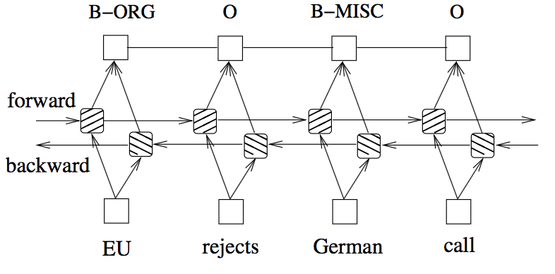
To the best of our knowledge, this was the first work to apply a bidirectional-LSTM-CRF architecture for sequence tagging. The idea is to use two LSTMs, one reading each word in a sentence from beginning to end and another reading the same but from end to beginning, producing for each word, a vector representation made from both the un-folded LSTM (i.e., forward and backward) read up to that word. There is this intuition that the vector for each word will take into account the words read/seen before, on both directions.
-
There is no explicit mention in the paper on how the vectors from each LSTM are combined to produce a single vector for each word, I will assume that they are just concatenated.
-
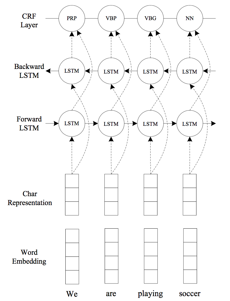
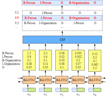
This bidirectional-LSTM architecture is then combined with a CRF layer at the top. A Conditional Random Field (CRF) layer has a state transition matrix as parameters, which can be used to efficiently use past attributed tags in predicting the current tag. The following diagram from Huang et al. (2015) shows a bi-LSTM-CRF model for NER.
Features and Embeddings
- Word embeddings generated from each state of the LSTM, are combined with hand-crafted features:
- spelling, e.g.: capitalization, punctuation, word patters, etc.
- context, e.g: uni-, bi- and tri-gram features
- The embeddings used are those produced by Collobert et al., 2011 which has 130K vocabulary size and each word corresponds to a 50-dimensional embedding vector.
Features connection tricks
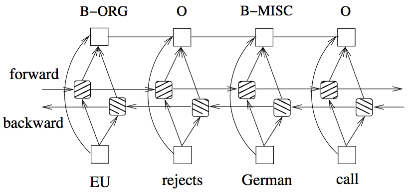
- The input for the model include both word, spelling and context features, however, the authors suggest direct connecting the hand-crafted features to the output layer (i.e, CRF) which accelerates training and result in very similar tagging accuracy, when comparing without direct connections. That is, in my understanding, the vector representing the hand-crafted features are passed directly to the CRF and are not passed through the bidirectional-LSTM. The following diagram from Huang et al. (2015) shows a bi-LSTM-CRF model with Maximum Entropy features.
Summary
In essence, I guess one can see this architecture as using the output of the bidirectional-LSTM, vector representations for each word in a sentence, together with a vector of features derived from spelling and context hand-crafted rules, these vectors are concatenated and passed to a CRF layer.
Named Entity Recognition with Bidirectional LSTM-CNNs (2016)
Architecture
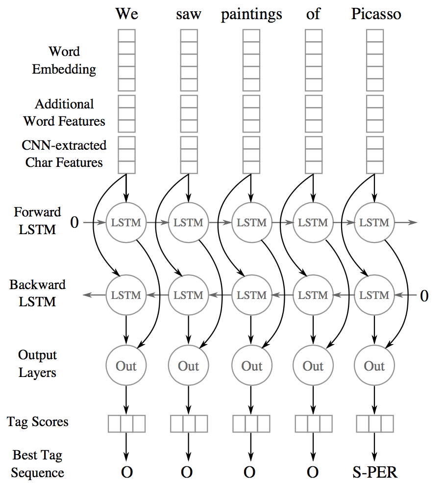
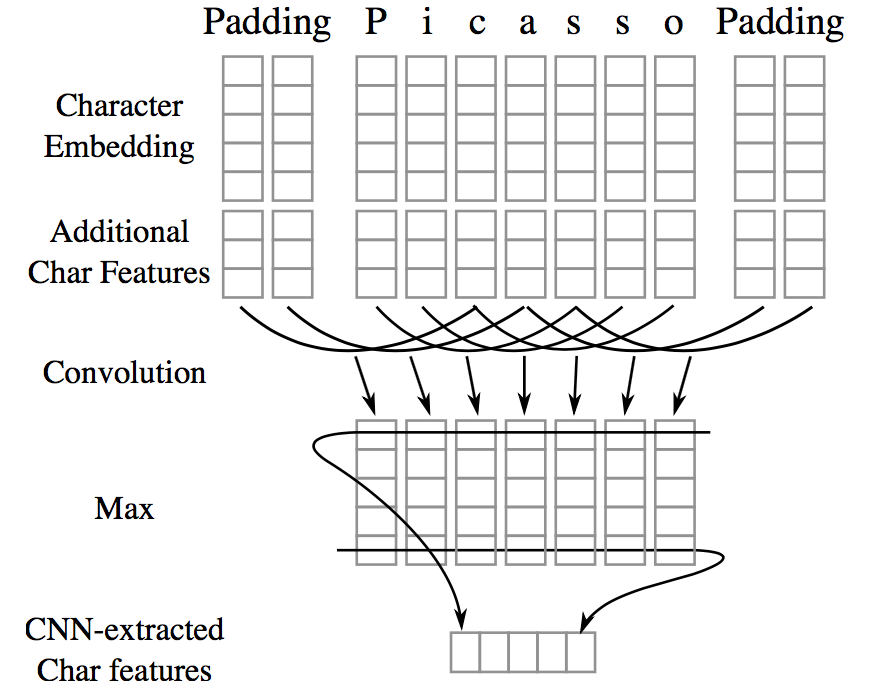
- The authors propose a hybrid model combining bidirectional-LSTMs with a Convolutional Neural Network (CNN), the latter learns both character- and word-level features. So, this makes use of words-embeddings, additional hand-crafted word features, and CNN-extracted character-level features. All these features, for each word, are fed into a bidirectional-LSTM. The following diagram from Chiu and Nichols (2016) shows a bidirectional-LSTMs with CNNs.
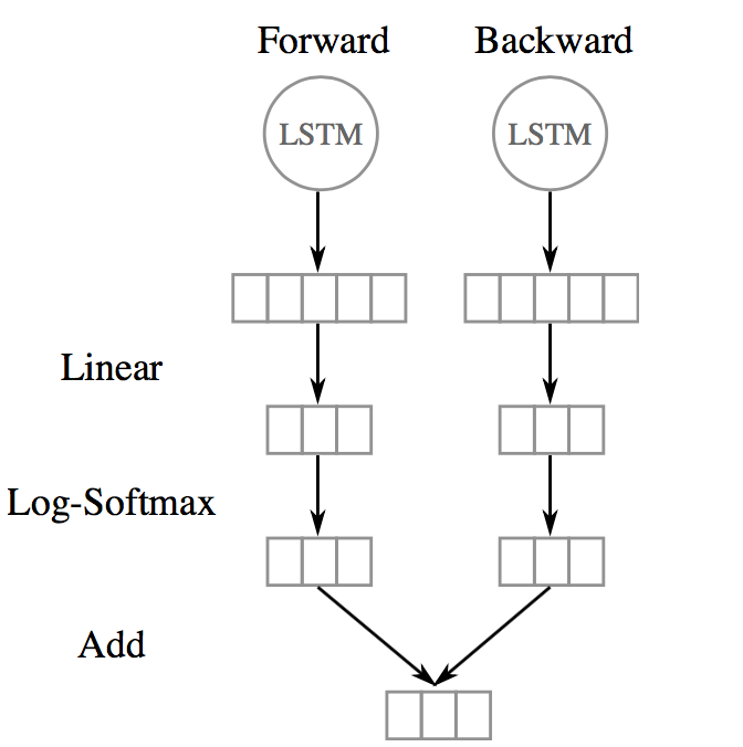
- The output vector of each LSTM (i.e., forward and backward) at each time step is decoded by a linear layer and a log-softmax layer into log-probabilities for each tag category, and These two vectors are then added together. The following diagram from Chiu and Nichols (2016) shows the output layer.
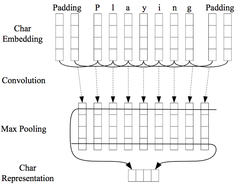
- Character-level features are induced by a CNN architecture, which was successfully applied to Spanish and Portuguese NER by Santos et al. (2015) and German POS-tagging by Labeau et al. (2015). For each word a convolution and a max layer are applied to extract a new feature vector from the per-character feature vectors such as character embeddings and character type. The following diagram from Chiu and Nichols (2016) shows the char-embeddings architecture.
Features and Embeddings
- Word Embeddings: 50-dimensional word embeddings by Collobert et al. (2011), all words are lower-cased, embeddings are allowed to be - modified during training.
- Character Embeddings: randomly initialized a lookup table with values drawn from a uniform distribution with range [−0.5,0.5] to output a character embedding of 25 dimensions. Two special tokens - are added: PADDING and UNKNOWN.
- Additional Char Features A lookup table was used to output a 4-dimensional vector representing the type of the character (upper case, lower case, punctuation, other).
- Additional Word Features: each words is tagged as allCaps, upperInitial, lowercase, mixedCaps, noinfo.
- Lexicons: partial lexicon matches using a list of known named-entities from DBpedia. The list is then used to perform \(n\)-gram matches against the words. A match is successful when the \(n\)-gram matches the prefix or suffix of an entry and is at least half the length of the entry.
Summary
-
The authors also explore several features, some hand-crafted:
- word embeddings
- word shape features
- character-level features (extracted with a CNN)
- lexical features
-
All these features are then concatenated, passed through a bi-LSTM and each time step is decoded by a linear layer and a log-softmax layer into log-probabilities for each tag category. The model also learns a tag transition matrix, and at inference time the Viterbi algorithm selects the sequence that maximizes the score all possible tag-sequences.
Implementations
Neural Architectures for Named Entity Recognition (2016)
Architecture
-
This was, to the best of my knowledge, the first work on NER to completely drop hand-crafted features, i.e., they use no language-specific resources or features beyond a small amount of supervised training data and unlabeled corpora.
-
Two architectures are proposed:
- Bidirectional LSTMs + Conditional Random Fields (CRF)
- Generating labels segments using a transition-based approach inspired by shift-reduce parsers
-
We shall focus on the first model, which follows a similar architecture as the other models presented in this post. The biggest selling point of this model is its simplicity.
-
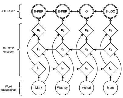
As in the previous models, two LSTMs are used to generate a word representation by concatenating its left and right context. These are two distinct LSTMs with different parameters. The tagging decisions are modeled jointly using a CRF layer by Lafferty et al. (2001). The following diagram from Lample et al. (2016) shows the model architecture.
Embeddings
-
The authors generate words embeddings from both representations of the characters of the word and from the contexts where the word occurs.
-
The rational behinds this idea is that many languages have orthographic or morphological evidence that a word or sequence of words is a named-entity or not, so they use character-level embeddings to try to capture these evidences. Secondly, named-entities appear in somewhat regular contexts in large corpora, therefore they use embeddings learned from a large corpus that are sensitive to word order.
Character Embeddings
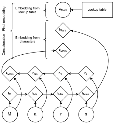
- A character lookup table is initialized randomly containing an embedding for every character. The character embeddings corresponding to every character in a word are given in direct and reverse order to a bidirectional-LSTM. The embedding for a word derived from its characters is the concatenation of its forward and backward representations from the bidirectional-LSTM. The hidden dimension of the forward and backward character LSTMs are 25 each. The following diagram from Lample et al. (2016) shows the character-embeddings Architecture.
Word Embeddings
-
This character-level representation is then concatenated with a word-level representation from pre-trained word embeddings. Embeddings are pre-trained using skip-n-gram (Ling et al., 2015), a variation of skip-gram that accounts for word order.
-
These embeddings are fine-tuned during training, and the authors claim that using pre-trained over randomly initialized ones results in performance improvements.
-
They also mention that they apply a dropout mask to the final embedding layer just before the input to the bidirectional LSTM observe a significant improvement in model’s performance after using dropout.
Summary
-
This model is relatively simple, the authors use no hand-crafted features, just embeddings. The word embeddings are the concatenation of two vectors, a vector made of character embeddings using two LSTMs, for each character in a word, and a vector corresponding to word embeddings trained on external data.
-
The embeddings for word each word in a sentence are then passed through a forward and backward LSTM, and the output for each word is then fed into a CRF layer.
Implementations
- https://github.com/glample/tagger
- https://github.com/Hironsan/anago
- https://github.com/achernodub/bilstm-cnn-crf-tagger
End-to-end Sequence Labelling via Bi-directional LSTM-CNNs-CRF (2016)
Architecture
- This system is very similar to the previous one. The authors use a Convolutional Neural Networks (CNN) to encode character-level information of a word into its character-level representation. Then combine character- and word-level representations and feed them into bidirectional LSTM to model context information of each word. Finally, the output vectors of BLSTM are fed to the CRF layer to jointly decode the best label sequence. The following diagram from Ma and Hovy (2016) shows the model architecture.
Embeddings
Character Embeddings
- The CNN is similar to the one in Chiu and Nichols (2015), the second system presented, except that they use only character embeddings as the inputs to CNN, without any character type features. A dropout layer is applied before character embeddings are input to CNN. The following diagram from Ma and Hovy (2016) shows the character-embeddings architecture.
Word Embeddings
- The word embeddings are the publicly available GloVe 100-dimensional embeddings trained on 6 billion words from Wikipedia and web text.
Summary
- This model follows basically the same architecture as the one presented before, being the only architecture change the fact that they use CNN to generate word-level char-embeddings instead of an LSTM.
Implementations
Key takeaways
-
The main lessons learned from these papers are:
- Use two LSTMs (forward and backward)
- CRF on the top/final layer to model tag transitions
- Final embeddings are a combinations of word and character embeddings
-
The following table summarizes the main characteristics of each of the models:
| Features | Architecture Resume | Structured Tagging | Embeddings | |
|---|---|---|---|---|
| Huang et al. (2015) | Yes |
bi-LSTM output vectors +
features vectors connected to CRF |
CRF | Collobert et al. (2011)
pre-trained 50-dimensions |
| Chiu and Nichols (2016) | Yes |
word embeddings + features vector
input to a bi-LSTM the output at each time step is decoded by a linear layer and a log-softmax layer into log-probabilities for each tag category |
Sentence-level log-likelihood |
- Collobert et al. 2011
- char-level embeddings extracted with a CNN |
| Lample et al. (2016) | No |
chars and word embeddings
input for the bi-LSTM output vectors are fed to the CRF layer to jointly decode the best label sequence |
CRF |
- char-level embeddings
extracted with a bi-LSTM - pre-trained word embeddings with skip-n-gram |
| Ma and Hovy (2016) | No |
chars and word embeddings
input for the bi-LSTM output vectors are fed to the CRF layer to jointly decode the best label sequence |
CRF |
- char embeddings extracted with a CNN
- word embeddings: GloVe 100-dimensions |
Extra: Why a Conditional Random Field at the top?
-
Having independent classification decisions is limiting when there are strong dependencies across output labels, since you decide the label for a word independently from the previous given tags.
-
For sequence labeling or general structured prediction tasks, it is beneficial to consider the correlations between labels in neighborhoods and jointly decode the best chain of labels for a given input sentence:
-
NER is one such task, since interpretable sequences of tags have constraints, e.g.: I-PER cannot follow B-LOC that would be impossible to model with independence assumptions;
-
Another example is in POS tagging, an adjective is more likely to be followed by a noun than a verb;
-
- The idea of using a CRF at the top is to model tagging decisions jointly, that is the probability of a given label to a word depends on the features associated to that word (i.e., final word embedding) and the assigned tag the word before.
- This means that the CRF layer could add constrains to the final predicted labels ensuring they are valid. The constrains are learned by the CRF layer automatically based on the annotated samples during the training process.
Emission score matrix
- The output of the LSTM is given as input to the CRF layer, that is, a matrix \(\textrm{P}\) with the scores of the LSTM of size \(n \times k\), where \(n\) is the number of words in the sentence and \(k\) is the possible number of labels that each word can have, \(\textrm{P}_{i,j}\) is the score of the \(j^{th}\) tag of the \(i^{th}\) word in the sentence. In the image below the matrix would be the concatenation of the yellow blocks coming out of each LSTM. The following diagram from https://createmomo.github.io shows the CRF Input Matrix.
Transition matrix
- \(\textrm{T}\) is a matrix of transition scores such that \(\textrm{P}_{i,j}\) represents the score of a transition from the tag \(i\) to tag \(j\). Two extra tags are added, \(y_{0}\) and \(y_{n}\) are the start and end tags of a sentence, that we add to the set of possible tags, \(\textrm{T}\) is therefore a square matrix of size \(\textrm{k}+2\). The following diagram from https://eli5.readthedocs.io shows the CRF State Transition Matrix.
![]()
Score of a prediction
-
For a given sequence of predictions for a sequence of words \(x\)…
\[\textrm{y} = (y_{1},y_{2},\dots,y_{n})\] -
…we can compute it’s score based on the emission and transition matrices:
\[\textrm{score}(y) = \sum_{i=0}^{n} \textrm{T}_{y_i,y_{i+1}} + \sum_{i=1}^{n} \textrm{P}_{i,y_i}\] -
So the score of a sequence of predictions is, for each word, the sum of the transition from the current assigned tag \(y_i\) to next assigned tag \(y_{i+1}\) plus the probability given by the LSTM to the tag assigned for the current word \(i\).
Training: parameter estimation
-
During training, we assign a probability to each tag but maximizing the probability of the correct tag \(y\) sequence among all the other possible tag sequences.
-
This is modeled by applying a softmax over all the possible taggings \(y\):
\[\textrm{p(y|X)} = \frac{e^{score(X,y)}}{\sum\limits_{y' \in Y({x})} e^{score(X,y')}}\]- where \(Y(x)\) denotes the set of all possible label sequences for \(x\), this denominator is also known as the partition function. So, finding the best sequence is the equivalent of finding the sequence that maximizes \(\textrm{score(X,y)}\).
-
The loss can be defined as the negative log likelihood of the current tagging \(y\):
- So, in simplifying the function above, a first step is to get rid of the fraction using log equivalences, and then get rid of the \(\textrm{log}\ e\) in the first term since they cancel each other out:
- Then the second term can be simplified by applying the log-space addition logadd, equivalence, i.e.: \(\oplus(a, b, c, d) = log(e^a+e^b+e^c+e^d)\):
- Then, replacing the \(\textrm{score}\) by it’s definition:
-
The first term is score for the true data. Computing the second term might be computationally expensive since it requires summing over the \(k^{n}\) different sequences in \(Y(x)\), i.e., the set of all possible label sequences for \(x\). This computation can be solved using a variant of the Viterbi algorithm, the forward algorithm.
-
The gradients are then computed using back-propagation, since the CRF is inside the neural-network. Note that the transition scores in the matrix are randomly initialized - or can also bee initialized based on some criteria, to speed up training - and will be updated automatically during your training process.
Inference: determining the most likely label sequence \(y\) given \(X\)
- Decoding is to search for the single label sequence with the largest joint probability conditioned on the input sequence:
- The parameters \(\theta\) correspond to the transition and emission matrices, basically the task is finding the best \(\hat{y}\) given the transition matrix \(\textrm{T}\) and the matrix \(\textrm{P}\) with scores for each tag for the individual word:
- A linear-chain sequence CRF model, models only interactions between two successive labels, i.e bi-gram interactions, therefore one can find the sequence \(y\) maximizing the score function above by adopting the Viterbi algorithm (Rabiner, 1989).
References
-
Bidirectional LSTM-CRF Models for Sequence Tagging (Huang et al. 2015)
-
Named Entity Recognition with Bidirectional LSTM-CNNs (Chiu and Nichols 2016)
-
Neural Architectures for Named Entity Recognition (Lample et al. 2016)
-
End-to-end Sequence Labelling via Bi-directional LSTM-CNNs-CRF (Ma and Hovy 2016)
-
A Tutorial on Hidden Markov Models and Selected Applications in Speech Recognition
-
Hugo Larochelle on-line lessons - Neural networks [4.1] : Training CRFs - loss function
-
Non-lexical neural architecture for fine-grained POS Tagging (Labeau et al., 2015)
-
Boosting Named Entity Recognition with Neural Character Embeddings (Santos et al., 2015)
Citation
If you found our work useful, please cite it as:
@article{Chadha2020NamedEntityRecognition,
  title   = {Named Entity Recognition},
  author  = {Chadha, Aman},
  journal = {Distilled AI},
  year    = {2020},
  note    = {\url{https://aman.ai}}
}