Primers • Convolutional Neural Networks for Text Classification
- Convolutional Neural Networks
- Convolutional Neural Networks for NLP
- Experiments and Results
- Summary
- References
- Citation
Convolutional Neural Networks
- Convolutional Neural Networks (ConvNets) have in the past years shown break-through results in some NLP tasks, one particular task is sentence classification, i.e., classifying short phrases (i.e., around 20 to 50 tokens), into a set of pre-defined categories. In this post I will explain how ConvNets can be applied to classifying short-sentences and how to easily implemented them in Keras.
- ConvNets were initially developed in the neural network image processing community where they achieved break-through results in recognizing an object from a pre-defined category (e.g., cat, bicycle, etc.).
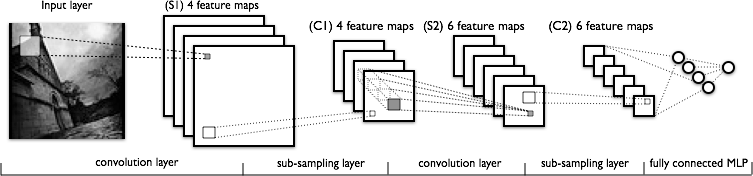
- A Convolutional Neural Network typically involves two operations, which can be though of as feature extractors: convolution and pooling.
- The output of this sequence of operations is then typically connected to a fully connected layer which is in principle the same as the traditional multi-layer perceptron neural network (MLP).
- The following diagram from Huang et al. (2015) shows a Convolutional Neural Network architecture applied to image classification.
Convolutions
- We can think about the input image as a matrix, where each entry represents each pixel, and a value between 0 and 255 representing the brightness intensity. Let’s assume it’s a black and white image with just one channel representing the grayscale. If you would be processing a colour image, and taking into account the colours one would have 3 channels, following the RGB colour mode.
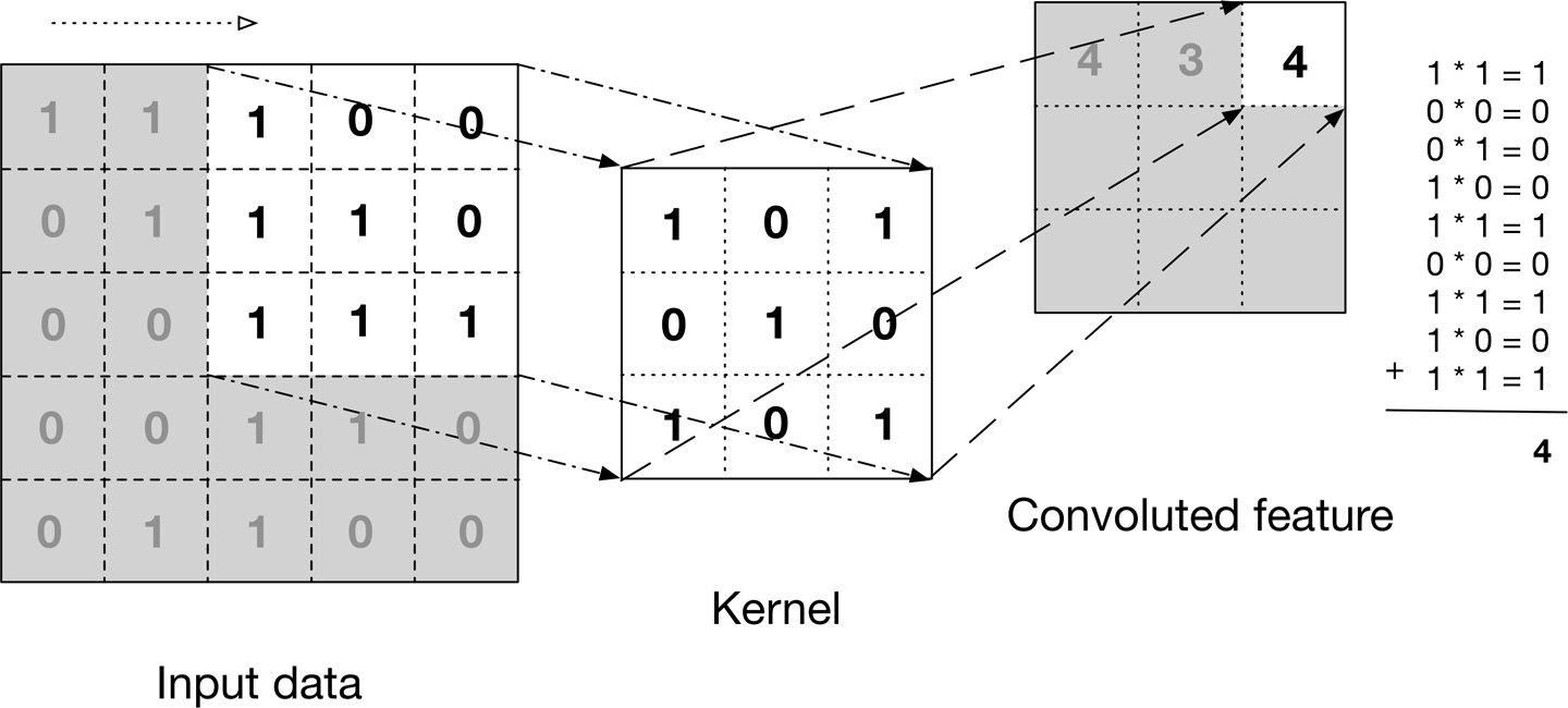
- One way to understand the convolution operation is to imagine placing the convolution filter or kernel on the top of the input image, positioned in a way so that the kernel and the image upper left corners coincide, and then multiplying the values of the input image matrix with the corresponding values in the convolution filter.
- All of the multiplied values are then added together resulting in a single scalar, which is placed in the first position of a result matrix.
- The kernel is then moved \(x\) pixels to the right, where \(x\) is denoted stride length and is a parameter of the ConvNet structure. The process of multiplication is then repeated, so that the next value in the result matrix is computed and filled.
- This process is then repeated, by first covering an entire row, and then shifting down the columns by the same stride length, until all the entries in the input image have been covered.
- The output of this process is a matrix with all it’s entries filled, called the convoluted feature or input feature map.
- An input image can be convolved with multiple convolution kernels at once, creating one output for each kernel.
- The following diagram from “Deep Learning” by Adam Gibson, Josh Patterson shows an example of a convolution operation.
Pooling
-
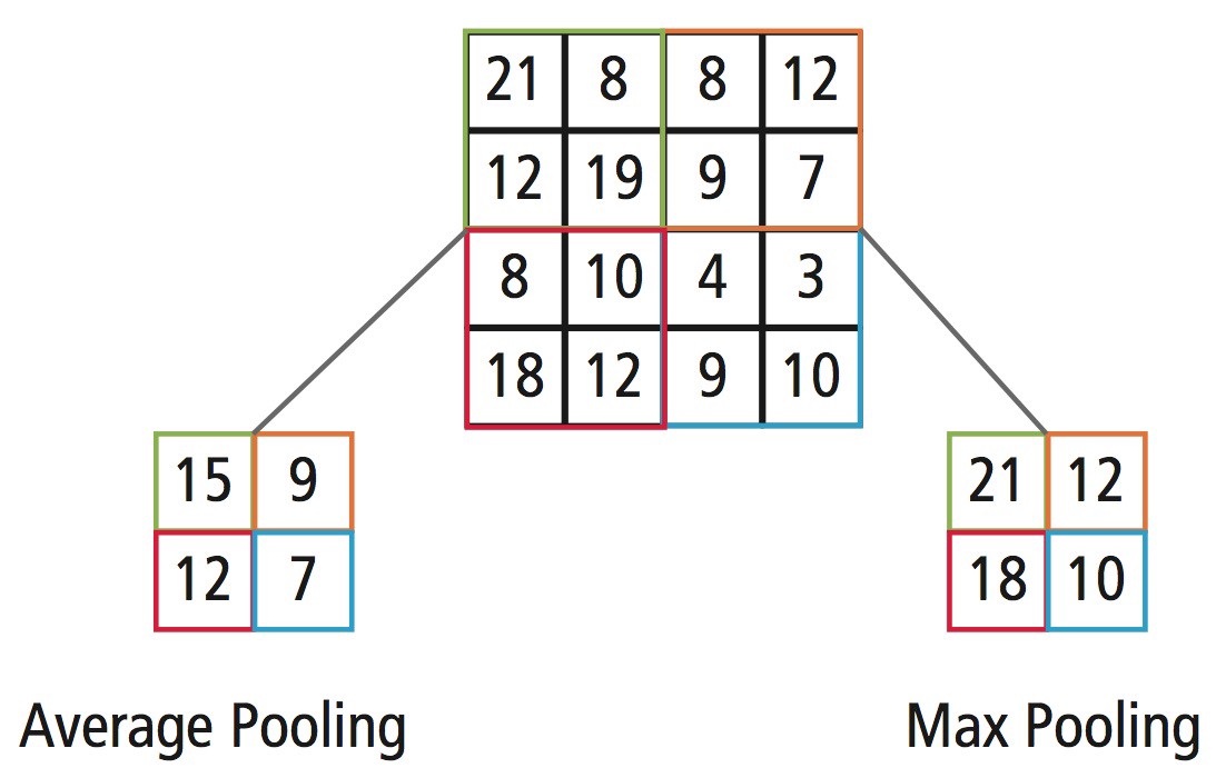
Next comes the pooling or downsampling layer, which consists of applying some operation over regions/patches in the input feature map and extracting some representative value for each of the analysed regions/patches.
-
This process is somehow similar to the convolution described before, but instead of transforming local patches via a learned linear transformation (i.e., the convolution filter), they’re transformed via a hardcoded operation.
- Two of the most common pooling operations are max- and average-pooling. Max-pooling selects the maximum of the values in the input feature map region of each step and average-pooling the average value of the values in the region. The output in each step is therefore a single scalar, resulting in significant size reduction in output size.
- The following diagram from AJ Cheng’s blog shows an example of a pooling operation with stride length of 2.
- Why do we downsample the feature maps and simply just don’t remove the pooling layers and keep possibly large feature maps? François Chollet in “Deep Learning with Python” summarises it well in this sentence:
“The reason to use downsampling is to reduce the number of feature-map coefficients to process, as well as to induce spatial-filter hierarchies by making successive convolution layers look at increasingly large windows (in terms of the fraction of the original input they cover).”
Fully Connected
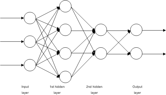
- The two processes described before, i.e., convolutions and pooling, can been thought of as a feature extractors, then we pass this features, usually as a reshaped vector of one row, further to the network, for instance, a multi-layer perceptron to be trained for classification. The following diagram shows an example of multi-layer perceptron network used to train for classification.
- This was a briefly description of the ConvNet architecture when applied to image processing, let’s now see how we can adapt this architecture to Natural Language Processing tasks.
Convolutional Neural Networks for NLP
- In the case of NLP tasks, i.e., when applied to text instead of images, we have a 1 dimensional array representing the text. Here the architecture of the ConvNets is changed to 1D convolutional-and-pooling operations.
- One of the most typically tasks in NLP where ConvNet are used is sentence classification, that is, classifying a sentence into a set of pre-determined categories by considering \(n\)-grams, i.e. it’s words or sequence of words, or also characters or sequence of characters.
1-D Convolutions over text
- Given a sequence of words \(w_{1:n} = w_{1}, \ldots, w_{n}\), where each is associated with an embedding vector of dimension \(d\). A 1D convolution of width-\(k\) is the result of moving a sliding-window of size \(k\) over the sentence, and applying the same convolution filter or kernel to each window in the sequence, i.e., a dot-product between the concatenation of the embedding vectors in a given window and a weight vector \(u\), which is then often followed by a non-linear activation function \(g\).
- Considering a window of words \(w_{i}, \ldots, w_{i+k}\) the concatenated vector of the \(i\)th window is then:
- The convolution filter is applied to each window, resulting in scalar values \(r_{i}\), each for the \(i\)th window:
-
In practice one typically applies more filters, \(u_{1}, \ldots, u_{l}\), which can then be represented as a vector multiplied by a matrix \(U\) and with an addition of a bias term \(b\):
\[\text{r}_{i} = g(x_{i} \cdot U + b)\]- with \(\text{r}_{i} \in R^{l},\ \ \ x_{i} \in R^{\ k\ \times\ d},\ \ \ U \in R^{\ k\ \cdot\ d \ \times l}\ \ \ \text{and}\ \ \ b \in R^{l}\)
-
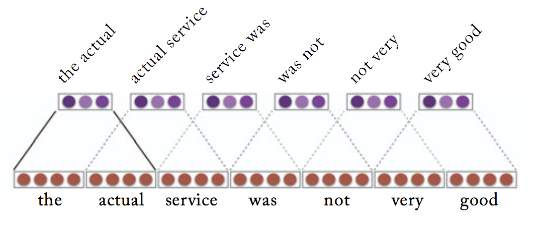
The following diagram from Yoav Goldberg’s book “Neural Network Methods for NLP” shows an example of a sentence convolution in a vector-concatenation notation with \(k\)=2 and dimensional output \(l\)=3.
Channels
-
In the introduction above we assumed we were processing a black and white image, and therefore we have one matrix representing the grayscale intensity of each pixel. With the RGB colour mode each pixel would be a combination of three intensity values instead, one for each of Red, Green and Blue components, and such representation would be stored in three different matrices, providing different characteristics or view of the image, referred to as a Channel. It’s common to apply a different set of filters to each channel, and then combine the three resulting vectors into a single vector.
-
We can also apply the multiple channels paradigm in text processing as well. For example, for a given phrase or window of text, one channel could be the sequence of words, a second channel could be the sequence of corresponding part-of-speech (POS) tags, and a third one could be the shape of the words:
| Word: | The | plane | lands | in | Lisbon |
|---|---|---|---|---|---|
| PoS-tag: | DET | NOUN | VERB | PROP | NOUN |
| Shape: | Xxx | xxxx | xxxx | xx | Xxxxxx |
- Applying the convolution over the words will result in \(m\) vectors \(w\), applying it over the PoS-tags will result also in \(m\) vectors, and the same for the shapes, again \(m\) vectors. These three different channels can then be combined either by summation:
- or by concatenation:
NOTE: each channel can still have different convolutions that read the source document using different kernel sizes, for instance, applying different context windows over words, pos-tags or shapes.
Pooling
- The pooling operation is used to combine the vectors resulting from different convolution windows into a single \(l\)-dimensional vector. This is done again by taking the max or the average value observed in resulting vector from the convolutions. Ideally this vector will capture the most relevant features of the sentence/document.
- This vector is then fed further down in the network - hence, the idea that ConvNet itself is just a feature extractor - most probably to a full connected layer to perform prediction.
Convolutional Neural Networks for Sentence Classification
-
We did a quick experiment, based on the paper by Y. Kim, implementing the four ConvNets models he used to perform sentence classification.
-
CNN-rand: all words are randomly initialized and then modified during training
-
CNN-static: pre-trained vectors with all the words— including the unknown ones that are randomly initialized—kept static and only the other parameters of the model are learned
-
CNN-non-static: same as CNN-static but word vectors are fine-tuned
-
CNN-multichannel: model with two sets of word vectors. Each set of vectors is treated as a channel and each filter is applied
-
-
Let’s just first quickly look at how these different models look like in as a computational graph. The first three (i.e., CNN-rand, CNN-static and CNN-non-static) look pretty much the same:

- The CNN-multichannel model uses two embedding layers, in one channel the embeddings are updated, in the second they remain static. It’s exactly the same network as above but duplicated and adding an extra layer do concatenate both results into a single vector:

Experiments and Results
-
We applied the implemented models on same of the datasets that Kim reported, but we could not get exactly the same results, first his results were reported over, we believe a TensorFlow implementation, and then there is the issue of how the datasets are pre-processed, i.e., tokenised, cleaned, etc.; that will always impact the results.
-
Another issue which puzzles me is that all those experiments only take into consideration the accuracy. Since the class samples are not uniformly distributed across the different classes, we think this is the wrong way to evaluate a classifier.
-
All the code for the models and experiments is available here.
Summary
-
The CNN is just a feature-extraction architecture, alone itself is not useful, but is the fist building block of a larger network. It needs to be trained together with a classification layer in order to produce some useful results.
-
As Yoav Goldberg summarizes it:
“The CNN layer’s responsibility is to extract meaningful sub-structures that are useful for the overall prediction task at hand. A convolutional neural network is designed to identify indicative local predictors in a large structure, and to combine them to produce a fixed size vector representation of the structure, capturing the local aspects that are most informative for the prediction task at hand. In NLP, the convolutional architecture will identify \(n\)-grams that are predictive for the task at hand, without the need to pre-specify an embedding vector for each possible ngram.”
- convolution: an operation which applies a filter to a fixed size window.
- convolution filter or kernel: a template matrix which is used in the convolution operation.
- pooling: combines the vectors resulting from different convolution windows into a single \(l\)-dimensional vector.
- feature_maps: the number of feature maps directly controls capacity and depends on the number of available examples and task complexity.
References
- “Convolutional Neural Networks for Sentence Classification” by Y. Kim (2014) in Conference on Empirical Methods in Natural Language Processing (EMNLP’14)
-
“Deep Learning” by Adam Gibson and Josh Patterson (2017), published by O’Reilly Media, Inc.
-
“Neural Network Methods for Natural Language Processing” by Yoav Goldberg (2017) published by Morgan & Claypool Publishers
- “Deep Learning with Python” by François Chollet (2017) published by Manning Publications
Citation
If you found our work useful, please cite it as:
@article{Chadha2020DistilledCNNsforTextClassification,
  title   = {Convolutional Neural Networks for Text Classification},
  author  = {Chadha, Aman},
  journal = {Distilled AI},
  year    = {2020},
  note    = {\url{https://aman.ai}}
}