Primers • Mixture of Experts
- Overview
- Motivation: Why Mixture-of-Experts?
- Mixture-of-Experts: The Classic Approach
- Hands-On Exercise: How does an MoE model work?
- The Deep Learning Way: Sparsely-Gated MoE
- The “How” Behind MoE
- Expert Capacity and Capacity Factor
- Load Balancing
- Token Dropping
- Expert Specialization
- Differentiability of Sparse Routing in Mixture-of-Experts
- Implementation
- Expert Choice Routing
- Mixture-of-Experts Beyond MLP Layers
- Beyond Token-based Routing: Structural and Hierarchical Routing Paradigms
- Expert Parallelism
- Limitations
- Inference-Time Memory Residency and VRAM Requirements (Primary Limitation)
- Training Instability and Load Imbalance
- Communication Overhead and Hardware Dependency
- Routing Complexity and Gradient Fragmentation
- Underutilization of Model Capacity
- Inference Instability and Latency Variability
- Additional Structural Challenges
- Popular MoE Models
- Learning Resources
- Related Papers
- Outrageously Large Neural Networks: The Sparsely-Gated Mixture-of-Experts Layer
- Scaling Vision with Sparse Mixture of Experts
- Modeling Task Relationships in Multi-task Learning with Multi-gate Mixture-of-Experts
- Mixture-of-Experts Meets Instruction Tuning: A Winning Combination for Large Language Models
- From Sparse to Soft Mixtures of Experts
- Switch Transformers
- QMoE: Practical Sub-1-Bit Compression of Trillion-Parameter Models
- MegaBlocks: Efficient Sparse Training with Mixture-of-Experts
- MoE-LLaVA: Mixture of Experts for Large Vision-Language Models
- Mixture of LoRA Experts
- JetMoE: Reaching Llama2 Performance with 0.1M Dollars
- QMoE: Practical Sub-1-Bit Compression of Trillion-Parameter Models
- CuMo: Scaling Multimodal LLM with Co-Upcycled Mixture-of-Experts
- Branch-Train-MiX: Mixing Expert LLMs into a Mixture-of-Experts LLM
- SwitchHead: Accelerating Transformers with Mixture-of-Experts Attention
- UMoE: Unifying Attention and FFN with Shared Experts
- Mixture of Attention Heads: Selecting Attention Heads Per Token
- Further Reading
- Citation
Overview
-
Neural networks have become the cornerstone of modern deep learning, providing a powerful mechanism for discovering complex patterns and extracting meaningful insights from massive datasets. However, the performance and expressiveness of such networks often scale with their parameter count — larger models tend to perform better but at the cost of exponentially increasing computational and memory demands.
-
Mixture-of-Experts (MoE) offers an elegant and efficient solution to this scaling bottleneck. Rather than activating all parameters for every input, MoE adopts a conditional computation paradigm — selectively activating only a small subset of “experts” based on the data. This approach allows models to achieve near-linear parameter scaling without a proportional increase in compute cost, making it a cornerstone of today’s ultra-large architectures.
-
The MoE concept was first introduced in Mixture of Experts by Jacobs et al. (1991), which established the foundational principles of “gating” and “experts.” The gating network, acting as a dynamic controller, decides which expert (or subset of experts) should handle a given input. Each expert, in turn, specializes in a particular region of the input space, enabling the ensemble to capture complex, heterogeneous data distributions more effectively than monolithic models. This early framework laid the groundwork for later developments in conditional computation and ensemble learning.
-
As deep learning matured, these ideas were revisited and dramatically scaled:
- The Sparsely-Gated Revolution:
- Outrageously Large Neural Networks: The Sparsely-Gated Mixture-of-Experts Layer by Shazeer et al. (2017) introduced top-\(k\) routing, a breakthrough mechanism that routes each input token through only the top \(k\) most relevant experts based on gating scores. This innovation drastically reduced computation while maintaining performance, making it feasible to train neural networks with billions of parameters. Additionally, the authors introduced load-balancing losses to ensure even expert utilization, mitigating the instability caused by uneven routing.
- Scaling with Simplicity:
- The Switch Transformer by Fedus et al. (2021) simplified the MoE architecture by using top-1 routing — assigning each token to a single expert instead of multiple ones. Despite this simplification, the Switch Transformer achieved state-of-the-art performance across large-scale NLP benchmarks while dramatically reducing communication overhead. It became a key stepping stone in scaling models like Google’s T5 family and influenced architectures underlying large-scale systems such as GPT and PaLM.
- Structured Sparsity and Efficiency:
- Building upon these advances, Dropless MoE by Gale et al. (2022) reformulated sparse MoE computation using block-sparse matrix multiplication, a paradigm implemented in the MegaBlocks system. This approach removed the need for token “dropping” and capacity constraints that limited earlier MoE implementations. As a result, MegaBlocks achieved both superior scaling efficiency and hardware utilization, representing one of the fastest industry-grade sparse MoE frameworks to date.
- The Sparsely-Gated Revolution:
-
Together, these works reflect the steady evolution of MoE architectures — from theoretical ensemble models in the early 1990s to the computational backbone of trillion-parameter systems in the 2020s. This three-decade journey demonstrates the field’s resilience and innovation, with each milestone bringing a new balance between scalability, efficiency, and specialization.
-
The infographic below (source) summarizes these milestones in the history of sparse MoE technology. It highlights how these innovations — from Jacobs’ early gating networks to Shazeer’s sparsely-gated layers and Fedus’s streamlined switch routing — have shaped the trajectory of scalable AI systems such as OpenAI’s GPT-4, Google’s Switch Transformer, and emerging multimodal MoEs. Together, they showcase a recurring theme: efficient specialization at scale — the central promise of the Mixture-of-Experts paradigm.

Modern Implementations: Hardware-Aware and Domain-Adaptive MoEs
- The following generation of research, exemplified by Dropless MoE by Gale et al. (2022), shifted focus toward hardware-aware sparsity. By reformulating MoE computation as block-sparse matrix operations, Dropless MoE (via the MegaBlocks framework) removed routing constraints and improved FLOPs utilization — allowing modern accelerators to exploit MoE sparsity efficiently. This efficiency breakthrough laid the foundation for industrial-scale distributed MoEs, particularly those powering multimodal and multilingual systems.
Influence on Next-Generation Models
-
Modern models such as Mixtral-8×7B, DeepSeek-V2, Gemini 1.5, and Claude 3 continue this lineage by embedding MoE principles not only in feed-forward layers but also in attention and cross-modal fusion mechanisms.
- Mixtral-8×7B by Mistral AI (2024) integrates expert routing across decoder blocks, combining the efficiency of sparse activation with the expressivity of dense transformers.
- DeepSeek-V2 extends MoE routing into multimodal alignment, using shared experts for vision-language fusion.
- Gemini 1.5 by Google DeepMind (2024) applies hierarchical expert routing to unify text, image, and code understanding — marking one of the first large-scale commercial systems to employ joint MoE across modalities.
The Continuing Trajectory
- Across these stages, the Mixture-of-Experts paradigm has evolved from an ensemble-learning curiosity into a core architectural principle of scalable intelligence. By selectively activating computation, MoEs align compute expenditure with information complexity — a concept increasingly central to the sustainability and interpretability of trillion-parameter AI systems.
- Future directions now explore structural routing, expert specialization across modalities, and dynamic compute allocation, heralding a new era of adaptable, efficient, and semantically aware expert networks.
Taxonomy of Modern MoE Architectures
- As Mixture-of-Experts architectures have evolved, researchers have introduced a variety of formulations tailored for efficiency, specialization, and scalability across modalities and tasks. Modern MoE systems can be organized into several key categories—each representing a distinct approach to expert routing, activation, and integration within large-scale models.
Sparse MoE Architectures
-
Sparse MoE models activate only a small subset of experts for each input, achieving massive parameter scaling while maintaining computational efficiency.
- Switch Transformer by Fedus et al. (2021) exemplifies this paradigm, using top-1 routing to send each token to a single expert.
- GLaM by Du et al. (2021) extends this with balanced token-to-expert assignments and importance-weighted routing.
- Mixtral-8×7B by Mistral AI (2024) improves upon Switch’s efficiency with optimized load balancing and routing parallelism.
-
Key property: Sparse activation ensures that only a fraction of model parameters are active per token, making these architectures ideal for large-scale pretraining.
Dense–Hybrid MoE Architectures
-
Dense–Hybrid models blend the efficiency of sparse MoE layers with the robustness of dense transformer blocks. They selectively introduce MoE layers into deeper or more specialized parts of the network.
- T5-MoE by Zoph et al. (2022) incorporates sparse experts within the feed-forward layers of T5, combining dense attention with sparse computation.
- DeepSeek-V2 introduces hybrid routing within both encoder and decoder stacks, adapting expert utilization based on modality and context complexity.
-
Key property: Hybrid models retain the stability of dense layers while exploiting MoE sparsity for scaling efficiency.
Hierarchical and Structured MoE Architectures
-
Hierarchical MoEs introduce multiple layers or levels of routing, enabling structured specialization. Experts can operate at different semantic or abstraction levels (e.g., local vs. global).
- Hierarchical Mixture of Experts (HMoE) by Zhou et al. (2022) models expert hierarchies explicitly, allowing high-level experts to coordinate low-level ones.
- Sparse-Transformer++ by Xu et al. (2025) implements multi-stage routing—first among global experts, then among local sub-experts—enhancing interpretability and specialization.
- HC-SMoE by Chen et al. (2025) clusters experts post-training using hierarchical clustering, merging redundant experts without retraining.
-
Key property: These models enable multi-granular routing, improving efficiency and interpretability across hierarchical representations.
Joint MoE and Multimodal Architectures
-
In multimodal MoE systems, both attention and feed-forward components are expert-based, allowing cross-modal interaction and dynamic parameter sharing.
- Uni-MoE by Li et al. (2024) jointly routes text and vision tokens through shared experts, unifying multimodal learning.
- Union of Experts by Yang et al. (2025) employs hierarchical routing where global experts manage modality fusion, while local experts refine within-modality reasoning.
-
Key property: Joint MoEs exploit shared structure across modalities, enabling scalable multimodal reasoning and cross-domain generalization.
Adaptive and Dynamic MoE Architectures
-
These architectures dynamically adjust the number of active experts or routing intensity based on input complexity or importance.
- AdaMoE by Zeng et al. (2024) introduces token-adaptive routing with null experts, which skip computation for trivial tokens.
- Expert Choice Routing (EC-MoE) by Zhou et al. (2022) reverses the routing direction—allowing experts to choose tokens—achieving better load balancing and conceptual clustering.
-
Key property: Adaptive MoEs align compute allocation with token complexity, improving efficiency and semantic coherence.
Modern MoE Landscape
| Type | Representative Models | Routing Mechanism | Key Advantage |
|---|---|---|---|
| Sparse | Switch Transformer, GLaM, Mixtral | Top-k token routing | Extreme scalability |
| Dense–Hybrid | T5-MoE, DeepSeek-V2 | Partial MoE integration | Stability + efficiency |
| Hierarchical | HMoE, Sparse-Transformer++, HC-SMoE | Multi-level expert routing | Interpretability, multi-scale reasoning |
| Joint / Multimodal | Uni-MoE, Union of Experts | Cross-modal routing | Unified multimodal processing |
| Adaptive / Dynamic | AdaMoE, EC-MoE | Token- or expert-adaptive | Compute proportional to complexity |
- In essence, modern MoE systems are evolving from simple token-wise routers into hierarchically organized, multimodal, and adaptive ecosystems of experts. This taxonomy captures the expanding design space of MoEs — from sparse parameter efficiency to cross-modal intelligence — underscoring their central role in next-generation AI architectures.
Motivation: Why Mixture-of-Experts?
The scaling bottleneck of dense neural networks
-
Modern deep learning has been driven by a clear empirical trend: increasing model capacity improves performance when sufficient data and optimization stability are available. This pattern underlies the success of large Transformer-based models such as BERT by Devlin et al. (2018), GPT-3 by Brown et al. (2020), and PaLM by Chowdhery et al. (2022). However, dense scaling suffers from a fundamental inefficiency: all parameters are activated for every token.
-
As model size grows, this dense activation regime causes training and inference costs to rise sharply, not only due to increased FLOPs but also because of memory bandwidth pressure, inter-device communication, and synchronization overheads. Shazeer et al. explicitly describe this issue as a “quadratic blow-up” when both model size and dataset size increase in dense architectures (Outrageously Large Neural Networks: The Sparsely-Gated Mixture-of-Experts Layer by Shazeer et al. (2017)). This dense-activation regime quickly becomes economically and physically infeasible at trillion-parameter scale.
-
The core challenge is therefore not a lack of representational power, but the inability of dense architectures to scale computation efficiently with model capacity.
Conditional computation as a principled solution
-
Mixture-of-Experts (MoE) architectures address this challenge by introducing conditional computation. Rather than executing the full network for every token, an MoE model activates only a small subset of specialized sub-networks (experts), selected dynamically by a learned routing function.
-
This idea traces back to early modular and ensemble methods such as Adaptive Mixtures of Local Experts by Jacobs et al. (1991) and was later formalized in deep learning contexts through conditional computation frameworks like Conditional Computation in Neural Networks by Bengio et al. (2013).
-
Formally, given a token representation \(x\), a router produces a sparse gating vector \(g(x) \in \mathbb{R}^N\) over \(N\) experts, and only the top-\(k\) experts are evaluated:
\[y(x) = \sum_{i \in \text{Top-}k(g(x))} g_i(x), f_i(x)\]- where \(f_i\) denotes the \(i^{th}\) expert network.
-
This mechanism decouples model capacity from per-token compute, enabling models to grow in parameter count without incurring a proportional increase in computational cost.
Scaling training with sparse activation
-
The primary training advantage of MoE lies in compute-efficient scaling. By activating only a small fraction of parameters per token, MoE models can dramatically increase total parameter count while keeping training FLOPs nearly constant relative to a dense baseline.
-
The sparsely-gated MoE layer introduced by Shazeer et al. (2017) demonstrated that it is possible to train models with orders-of-magnitude more parameters than dense Transformers, while maintaining similar training throughput. This insight was extended to large-scale distributed systems by GShard by Lepikhin et al. (2020), which showed that expert parameters could be sharded across thousands of accelerators and trained jointly using sparse routing.
-
Further simplification came from Switch Transformers by Fedus et al. (2021), which demonstrated that routing each token to a single expert is sufficient to retain model quality while substantially reducing communication overhead. These results established sparse MoE as a practical path to training trillion-parameter models.
-
In effect, MoE allows training compute to scale with the number of active experts per token rather than the total number of parameters, fundamentally altering the economics of large-scale pretraining.
Training efficiency and expert specialization
-
From a learning perspective, MoE enables specialization without explicit supervision. Empirical evidence suggests that experts self-organize around latent structures in the data, such as syntax, domain, or modality (Towards Understanding Mixture of Experts in Deep Learning by Chen et al. (2022)). Because each expert processes a narrower distribution of inputs, gradients are less noisy and convergence can be faster than in dense counterparts of comparable quality.
-
This specialization effect becomes especially important in multilingual, multimodal, and instruction-tuned models, as demonstrated in GLaM by Du et al. (2021), Mixtral of Experts by Jiang et al. (2024), and MoE-LLaVA by Xu et al. (2024).
-
In large-scale pretraining regimes, this implicit specialization improves representational efficiency by reducing interference between unrelated patterns, allowing different experts to focus on distinct subspaces of the data distribution while sharing a common embedding and attention backbone.
Efficient inference through conditional routing
-
At inference time, MoE architectures provide a compelling quality–cost trade-off. Although the total parameter count may be extremely large, inference cost per token depends only on the number of activated experts, not on the full model size.
-
This enables MoE models to achieve performance comparable to very large dense models while maintaining inference latency closer to that of much smaller networks. As a result, MoE is particularly attractive for deployment scenarios where throughput and cost efficiency are critical.
-
Moreover, conditional routing allows computation to adapt to input complexity. Simple or redundant tokens can be handled by a small subset of experts, while more complex tokens may engage more specialized computation paths. This form of adaptive inference is fundamentally unavailable in fully dense architectures.
Why MoE enables scalable neural networks
-
Taken together, Mixture-of-Experts architectures provide a structural solution to the scaling limits of dense neural networks. By introducing sparsity at the level of parameter activation, MoE enables:
- massive increases in model capacity without proportional training cost,
- improved representational efficiency through expert specialization,
- inference costs that scale with active computation rather than total parameters,
- adaptive computation aligned with input complexity.
-
As summarized in A Comprehensive Survey of Mixture-of-Experts by Jiang et al. (2025), MoE has evolved from an ensemble-learning technique into a central architectural principle for large-scale neural networks. Its success reflects a broader shift away from uniform computation toward models that allocate resources dynamically—making MoE a cornerstone of scalable training and inference in next-generation AI systems.
Mixture-of-Experts: The Classic Approach
- The MoE concept is a type of ensemble learning technique initially developed within the field of artificial neural networks. It introduces the idea of training experts on specific subtasks of a complex predictive modeling problem.
- In a typical ensemble scenario, all models are trained on the same dataset, and their outputs are combined through simple averaging, weighted mean, or majority voting. However, in an MoE architecture, each “expert” model within the ensemble is only trained on a subset of data where it can achieve optimal performance, thus narrowing the model’s focus. Put simply, MoE is an architecture that divides input data into multiple sub-tasks and trains a group of experts to specialize in each sub-task. These experts can be thought of as smaller, specialized models that are better at solving their respective sub-tasks.
- The popularity of MoE only rose recently as the appearance of Large Language Models (LLMs) and transformer-based models in general swept through the machine learning field. Consequently, this is because of modern datasets’ increased complexity and size. Each dataset contains different regimes with vastly different relationships between the features and the labels.
- To appreciate the essence of MoE, it is crucial to understand its architectural elements:
- Division of dataset into local subsets: First, the predictive modeling problem is divided into subtasks. This division often requires domain knowledge or employs an unsupervised clustering algorithm. It’s important to clarify that clustering is not based on the feature vectors’ similarities. Instead, it’s executed based on the correlation among the relationships that the features share with the labels.
- Expert Models: These are the specialized neural network layers or experts that are trained to excel at specific sub-tasks. Each expert receives the same input pattern and processes it according to its specialization. Put simply, an expert is trained for each subset of the data. Typically, the experts themselves can be any model, from Support Vector Machines (SVM) to neural networks. Each expert model receives the same input pattern and makes a prediction.
- Gating Network (Router): The gating network, also called the router, is responsible for selecting which experts to use for each input data. It works by estimating the compatibility between the input data and each expert, and then outputs a softmax distribution over the experts. This distribution is used as the weights to combine the outputs of the expert layers. Put simply, this model helps interpret predictions made by each expert and decide which expert to trust for a given input.
- Pooling Method: Finally, an aggregation mechanism is needed to make a prediction based on the output from the gating network and the experts.
- The gating network and expert layers are jointly trained to minimize the overall loss function of the MoE model. The gating network learns to route each input to the most relevant expert layer(s), while the expert layers specialize in their assigned sub-tasks.
- This divide-and-conquer approach effectively delegates complex tasks to experts, enabling efficient processing and improved accuracy. Together, these components ensure that the right expert handles the right task. The gating network effectively routes each input to the most appropriate expert(s), while the experts focus on their specific areas of strength. This collaborative approach leads to a more versatile and capable overall model.
- In summary, MoEs improve efficiency by dynamically selecting a subset of model parameters (experts) for each input. This architecture allows for larger models while keeping computational costs manageable by activating only a few experts per input.
Put simply, MoE is how an ensemble of AI models decides as one. It is basically multiple “experts”, i.e., individual models, in a “trend coat”.
Top-level Intuition
- MoE leverages multiple specialized models (experts) to solve complex tasks by dividing the problem space. Each expert becomes proficient in a specific subset of the data, leading to more efficient learning and problem-solving.
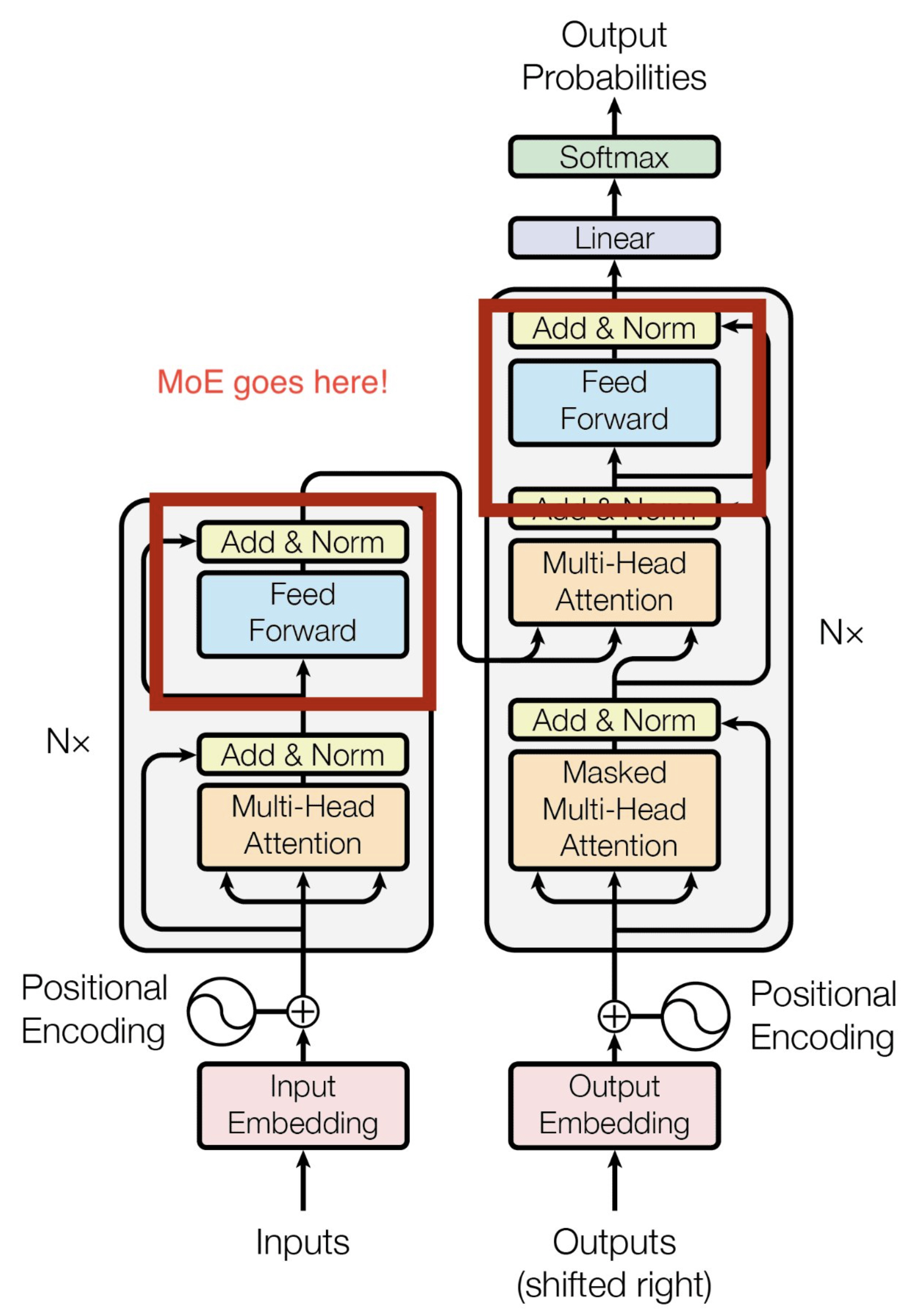
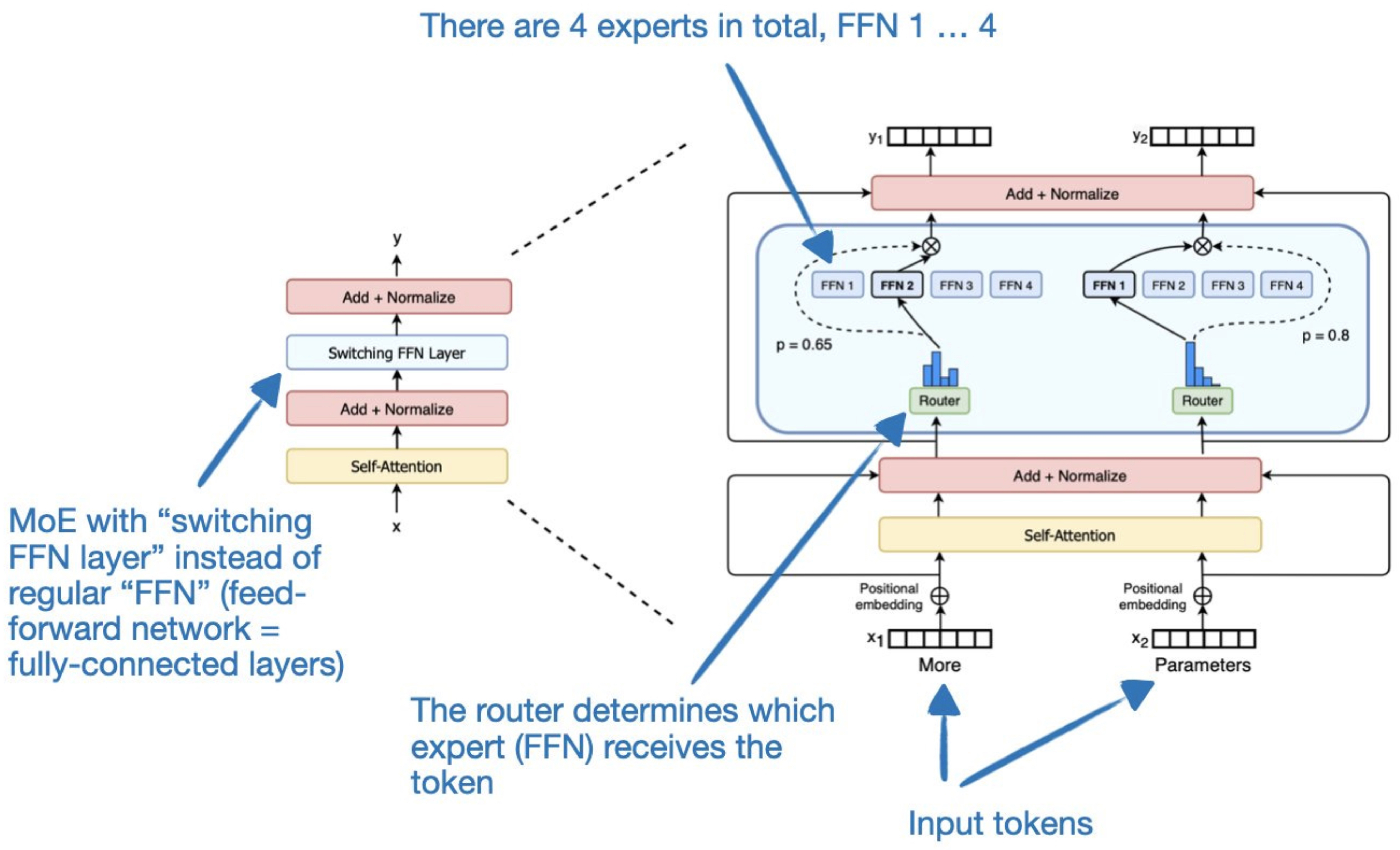
- Specifically, in the feed-forward parts of the model (not the attention blocks) the router selects an expert layer for every token. In the architecture proposed in the seminal paper Outrageously Large Neural Networks: The Sparsely-Gated Mixture-of-Experts Layer, within the feed-forward components of the model (excluding the attention blocks), the router assigns an expert layer for each token. The figures below (source: Nathan Lambert’s tweet, the Transformers and Switch Transformers paper) illustrates this feed-forward-based MoE architecture.
- Conversely, recent publications such as JetMoE: Reaching Llama2 Performance with 0.1M Dollars have expanded this approach, modeling both feed-forward and attention blocks as MoEs.
- A gating network determines which expert(s) to activate for a given input, ensuring the most relevant expertise is applied. The gate learns to assign inputs to experts dynamically, optimizing performance based on the task’s needs.
- MoE architectures reduce computational cost by only activating a subset of experts for each input, rather than the entire model. This approach allows for scalability and adaptability, making MoE suitable for large-scale and diverse datasets.
Gate Functionality
- This section seeks to answer how the gating network (also called gate, router, or switch) in MoE models works under the hood.
- Let’s explore two distinct but interconnected functions of the gate in a MoE model:
- Clustering the Data: In the context of an MoE model, clustering the data means that the gate is learning to identify and group together similar data points. This is not clustering in the traditional unsupervised learning sense, where the algorithm discovers clusters without any external labels. Instead, the gate is using the training process to recognize patterns or features in the data that suggest which data points are similar to each other and should be treated similarly. This is a crucial step because it determines how the data is organized and interpreted by the model.
- Mapping Experts to Clusters: Once the gate has identified clusters within the data, its next role is to assign or map each cluster to the most appropriate expert within the MoE model. Each expert in the model is specialized to handle different types of data or different aspects of the problem. The gate’s function here is to direct each data point (or each group of similar data points) to the expert that is best suited to process it. This mapping is dynamic and is based on the strengths and specialties of each expert as they evolve during the training process.
- In summary, the gate in an MoE model is responsible for organizing the incoming data into meaningful groups (clustering) and then efficiently allocating these groups to the most relevant expert models within the MoE system for further processing. This dual role of the gate is critical for the overall performance and efficiency of the MoE model, enabling it to handle complex tasks by leveraging the specialized skills of its various expert components.
Hands-On Exercise: How does an MoE model work?
- Credits to Tom Yeh for this exercise.
- Let’s calculate an MoE model by hand, with the following config: (i) number of experts: 2, (ii) tokens: 2, (iii) sparse.
- Step-by-step walkthrough:
- The MoE block receives two tokens (blue, orange).
- Gate Network processes \(X_1\) (blue) and determined \(\text{Expert}_2\) should be activated.
- \(\text{Expert}_2\) processes \(X_1\) (blue).
- Gate Network processes \(X_2\) (orange) and determined \(\text{Expert}_1\) should be activated.
- \(\text{Expert}_1\) processes \(X_2\) (orange).
- ReLU activation function processes the outputs of the experts and produces the final output.
Key Benefits
- Size: The model can get really large (while still being efficient, as highlighted in the next point) simply by adding more experts. In this example, adding one more expert means adding 16 more weight parameters.
- Efficiency: The gate network will select a subset of experts to actually compute, in the above exercise: one expert. In other words, only 50% of the parameters are involved in processing a token.
The Deep Learning Way: Sparsely-Gated MoE
- In 2017, an extension of the MoE paradigm suited for deep learning was proposed by Shazeer et al. in Outrageously Large Neural Networks: The Sparsely-Gated Mixture-of-Experts Layer.
- In most deep learning models, increasing model capacity generally translates to improved performance when datasets are sufficiently large. Generally, when the entire model is activated by every example, it can lead to “a roughly quadratic blow-up in training costs, as both the model size and the number of training examples increase”, stated by Shazeer et al. (2017).
- Although the disadvantages of dense models are clear, there have been various challenges for an effective conditional computation method targeted toward modern deep learning models, mainly for the following reasons:
- Modern computing devices like GPUs and TPUs perform better in arithmetic operations than in network branching.
- Larger batch sizes benefit performance but are reduced by conditional computation.
- Network bandwidth can limit computational efficiency, notably affecting embedding layers.
- Some schemes might need loss terms to attain required sparsity levels, impacting model quality and load balance.
- Model capacity is vital for handling vast data sets, a challenge that current conditional computation literature doesn’t adequately address.
- The MoE technique presented by Shazeer et al. aims to achieve conditional computation while addressing the abovementioned issues. They could increase model capacity by more than a thousandfold while only sustaining minor computational efficiency losses.
- The authors introduced a new type of network layer called the “Sparsely-Gated MoE Layer.” They are built on previous iterations of MoE and aim to provide a general-purpose neural network component that can be adapted to different types of tasks.
- The Sparsely-Gated MoE architecture (henceforth, referred to as the MoE architecture), consists of numerous expert networks, each being a simple feed-forward neural network and a trainable gating network. The gating network is responsible for selecting a sparse combination of these experts to process each input.

- The fascinating feature here is the use of sparsity in the gating function. This means that for every input instance, the gating network only selects a few experts for processing, keeping the rest inactive. This sparsity and expert selection is achieved dynamically for each input, making the entire process highly flexible and adaptive. Notably, the computational efficiency is preserved since inactive parts of the network are not processed.
- The MoE layer can be stacked hierarchically, where the primary MoE selects a sparsely weighted combination of “experts.” Each combination utilizes a MoE layer.
- Moreover, the authors also introduced an innovative technique called Noisy Top-\(K\) Gating. This mechanism adds a tunable Gaussian noise to the gating function, retains only the top \(k\) values, and assigns the rest to negative infinity, translating to a zero gating value. Such an approach ensures the sparsity of the gating network while maintaining robustness against potential discontinuities in the gating function output. Interestingly, it also aids in load balancing across the expert networks.
- In their framework, both the gating network and the experts are trained jointly via back-propagation, the standard training mechanism for neural networks. The output from the gating network is a sparse, n-dimensional vector, which serves as the gate values for the n-expert networks. The output from each expert is then weighted by the corresponding gating value to produce the final model output.
- The Sparse MoE architecture has been a game-changer in LLMs, allowing us to scale up modeling capacity with almost constant computational complexity, resulting breakthroughs such as the Switch Transformer, GPT-4, Mixtral-8x7b, and more.
The “How” Behind MoE
- Although the success of MoE is clear in the deep learning field, as with most things in deep learning, our understanding of how it can perform so well is rather unclear.
- Notably, each expert model is initialized and trained in the same manner, and the gating network is typically configured to dispatch data equally to each expert. Unlike traditional MoE methods, all experts are trained jointly with the MoE layer on the same dataset. It is fascinating how each expert can become “specialized” in their own task, and experts in MoE do not collapse into a single model.
- Towards Understanding Mixture of Experts in Deep Learning by Chen et al. attempts to interpret the “how” behind the MoE layers. They conclude that the “cluster structure of the underlying problem and the non-linearity of the expert is pivotal to the success of MoE.”
- Although the conclusion does not provide a direct answer, it helps to gain more insight into the simple yet effective approach of MoE.
Expert Capacity and Capacity Factor
Overview
-
In a MoE model, expert capacity defines the upper bound on how many tokens, samples, or activations may be routed to each expert during a training (or inference) step. This concept is essential for ensuring balanced expert utilization, computational efficiency, and stability in distributed training.
-
Although the foundational work on Sparsely-Gated MoE by Shazeer et al. (2017) introduced much of the routing mechanism, the explicit formalization of expert capacity and the associated capacity factor appear in later work — in particular in Switch Transformer, which defines expert capacity approximately as:
\[\text{expert_capacity} = \frac{T}{N} \times \alpha\]-
where:
- \(T\) is the number of tokens (or routed activations) in the batch,
- \(N\) is the number of experts, and
- \(\alpha\) is the capacity factor (a hyper-parameter)
-
Historical Context and Related Work
- The concept of expert capacity and its controlling hyper-parameter, the capacity factor, evolved through multiple generations of research in conditional computation and large-scale MoE models.
-
In summary:
-
Early conditional-computation research introduced sparse activation but lacked an explicit notion of capacity — for example, early adaptive computation work like Conditional Computation in Neural Networks by Bengio et al. (2013) discussed conditional activation without a formal capacity limit.
-
Outrageously Large Neural Networks: The Sparsely-Gated Mixture-of-Experts Layer by Shazeer et al. (2017) scaled sparse routing to hundreds of experts, revealing the need for explicit load control and motivating later formulations of expert capacity.
-
GShard: Scaling Giant Models with Conditional Computation and Automatic Sharding by Lepikhin et al. (2020) addressed large-scale MoE training and system-level scaling but treated expert capacity implicitly as an implementation-level constraint rather than a tunable hyper-parameter.
-
Switch Transformer: Scaling to Trillion Parameter Models with Simple and Efficient Sparsity by Fedus, Zoph & Shazeer (2021) formally defined the expert capacity equation and the capacity factor as explicit, first-class hyper-parameters.
-
Subsequent studies such as BASE Layers: Simplifying Training of Large, Sparse Models by Lewis et al. (2021), ST-MoE: Designing Stable and Transferable Sparse Expert Models by Zoph et al. (2022), and Efficient Large Language Models: A Survey by Dai et al. (2023) have expanded this idea into capacity-aware training and inference strategies — highlighting expert capacity as a controllable mechanism for efficiency, stability, and specialization.
-
- This evolution transformed expert capacity from a pragmatic load-balancing technique into a theoretically grounded and tunable component essential for scalable sparse neural networks, as reflected in later frameworks like Dropless MoE (MegaBlocks) by Kang et al. (2022) and Mixtral: Sparse Mixture of Experts by Jiang et al. (2024), which continue to refine capacity management in trillion-parameter architectures.
Early Conditional-Computation and MoE Origins
-
The notion of dividing computation among multiple experts dates back to early modular neural networks such as adaptive mixtures of local experts by Michael I. Jordan and Robert A. Jacobs (1991), described in Adaptive Mixtures of Local Experts. These early architectures introduced the idea of a gating network that learns how to distribute inputs to specialized sub-networks.
-
Later, conditional computation became central to deep learning research. According to Learning Factored Representations in a Deep Mixture of Experts by Eigen et al. (2013), the model proposed activating only subsets of a deep network for each input, foreshadowing the sparse-activation ideas used in modern MoE architectures. Similarly, Estimating or Propagating Gradients Through Stochastic Neurons for Conditional Computation by Bengio et al. (2015) extended this to stochastic routing, introducing probabilistic gating mechanisms that enabled selective activation of sub-networks.
-
These early efforts laid the groundwork for modern sparse expert activation but did not define an explicit per-expert token capacity or a capacity-factor hyper-parameter. That formalism would only emerge years later with large-scale transformer-based MoE systems.
The First Large-Scale Sparse MoE: “Sparsely-Gated MoE” (2017)
-
A major leap in scalability came with Outrageously Large Neural Networks: The Sparsely-Gated Mixture-of-Experts Layer by Shazeer et al. (2017). This seminal work operationalized Mixture-of-Experts at unprecedented scale, introducing thousands of feed-forward experts within Transformer-style architectures.
-
The key innovation was the sparsely-gated routing mechanism, where a learned gating network dynamically selected only the top-1 or top-2 experts for each input token. This selective activation made it possible to scale model size without linearly increasing computational cost.
-
The gating network was trained jointly with the experts and included an auxiliary load-balancing loss to encourage even expert utilization and prevent routing collapse (where a few experts dominate). The paper demonstrated how sparse activation could extend model capacity while maintaining manageable training costs on large distributed systems such as TensorFlow.
-
Despite these breakthroughs, the framework did not yet define a formal notion of expert capacity or a capacity factor. Instead, expert load control was managed heuristically through the gating loss and token-dropping mechanisms. These ideas laid the foundation for later work such as GShard and Switch Transformer, which explicitly quantified and parameterized per-expert capacity.
Scaling to Conditional Models: GShard (2020)
-
The next turning point in scaling conditional computation came with GShard. This system enabled training of multilingual Transformer models exceeding 600 billion parameters, establishing a new paradigm for distributed sparse computation across large clusters.
-
GShard introduced several key innovations that made large-scale sparse MoE training practical:
- Automatic sharding across thousands of devices, enabling each expert to reside on separate compute nodes while maintaining efficient communication via all-to-all token exchange.
- Top-2 routing, which improved stability compared to earlier top-1 gating, ensuring that each token could leverage two complementary experts.
- Dynamic load-balancing loss, inherited from Shazeer et al. (2017), to prevent expert overloading and under-utilization during distributed training.
-
While GShard significantly advanced the scalability of MoE systems, its treatment of expert capacity remained implicit. Each expert’s token processing limit was defined as a systems-level constant rather than a tunable model hyper-parameter. This approach worked for engineering stability but limited fine-grained control over computational balance and token overflow.
-
The insights from GShard directly influenced later developments such as Switch Transformer, which explicitly formulated the expert capacity equation and introduced the capacity factor (\(\alpha\)) as a first-class hyper-parameter governing token allocation per expert. This formalization transformed capacity management from a systems constraint into a learnable and optimizable design variable within large-scale MoE architectures.
Formalization of “Capacity Factor”: Switch Transformer (2021)
-
The formal definition of expert capacity emerged in Switch Transformers. This work extended the MoE paradigm to trillion-parameter scale while preserving training efficiency and stability. Its key contribution was the explicit mathematical formulation of expert capacity and the capacity factor, which collectively defined a tunable upper bound on how many tokens could be routed to each expert per training step.
-
The expert capacity \(C\) is defined as:
\[C = \frac{T}{N} \times \alpha\]-
where:
- \(T\) — total number of tokens in the batch,
- \(N\) — total number of experts,
- \(\alpha\) — capacity factor, a tunable scalar that expands or contracts per-expert token capacity.
-
-
The capacity factor \(\alpha\) was introduced to manage the natural variability in token-to-expert assignment. Since routing is probabilistic, some experts receive more tokens than others. Setting \(\alpha > 1\) provides a buffer to accommodate these fluctuations, while \(\alpha < 1\) enforces stricter token limits, increasing efficiency at the risk of dropping excess tokens.
-
According to Switch Transformers, “A capacity factor greater than 1.0 creates additional buffer to accommodate when tokens are not perfectly balanced across experts.” This insight formally linked the idea of routing imbalance to a controllable hyper-parameter, enabling model designers to trade off between computational efficiency, overflow tolerance, and token drop rates.
-
This formulation also introduced a deterministic rule for dropped tokens — when a particular expert exceeds its capacity \(C\), the overflow tokens are either skipped (via residual pathways) or rerouted to other experts, depending on the implementation. The result was a predictable and efficient routing framework that made trillion-parameter training feasible for the first time.
-
The explicit introduction of \(C\) and \(\alpha\) thus transformed what had previously been a system-level constraint (as in GShard) into a model-level hyper-parameter. This shift made expert capacity an essential design tool for controlling load balance, efficiency, and overall throughput in sparse architectures.
Subsequent Research: Variations and Deeper Analysis
-
Following the introduction of expert capacity and the capacity factor in Switch Transformer, subsequent research expanded the theoretical and empirical understanding of how these parameters affect efficiency, load balance, and convergence in MoE architectures.
-
According to A Comprehensive Survey of Mixture-of-Experts: Algorithms and Applications by Jiang et al. (2025), expert capacity and the capacity factor \(\alpha\) are “crucial for ensuring balanced load distribution and efficient utilization of the model’s experts.” This survey synthesizes evidence showing that proper tuning of \(\alpha\) directly improves FLOPs utilization and mitigates expert under-training, a phenomenon where certain experts receive insufficient tokens to learn meaningful specializations.
-
The Mixture-of-Experts with Expert Choice Routing by Zhou et al. (2022) explored the relationship between capacity and routing in detail. The authors demonstrated that lowering the capacity factor from 2.0 to 1.0 increased token drop rates, leading to performance degradation on language modeling benchmarks. Their experiments highlighted that balanced routing and sufficient per-expert capacity are essential for stable optimization and reduced gradient variance across experts.
-
Meanwhile, Capacity-Aware Inference: Mitigating the Straggler Effect in Mixture of Experts by He et al. (2025) focused on inference-time efficiency, proposing capacity-aware token dropping and rerouting mechanisms to avoid the “straggler effect,” where overloaded experts slow down batch inference. These methods adaptively monitor per-expert load and dynamically reassign tokens to maintain predictable latency, demonstrating that expert capacity also governs runtime stability, not just training efficiency.
-
Finally, industry practitioners and open-source frameworks have reinforced these insights. For example, Mixture-of-Experts Explained on the Hugging Face Blog emphasizes that setting the capacity factor between 1.0 and 1.25 achieves an optimal trade-off between throughput and overflow safety in top-2 routing configurations.
-
Collectively, these studies established expert capacity as a tunable control variable central to both system design and model convergence. It governs the interaction between routing stochasticity, memory provisioning, and distributed synchronization—making it one of the most practically significant hyper-parameters in large-scale MoE architectures.
Formal Definition and Role
- The formal notion of expert capacity was first articulated in Switch Transformers. This definition quantifies the number of tokens (or activations) each expert can process in a single forward pass, offering a mathematical framework for balancing computational efficiency and routing uniformity.
Definition
-
Suppose a MoE layer receives a batch of \(T\) tokens that are distributed among \(N\) experts. Each expert can handle at most \(C\) tokens per step, where \(C\) — the expert capacity — is defined as:
\[C = \frac{T}{N} \times \alpha\]-
where:
- \(T\) = total number of tokens in the batch,
- \(N\) = total number of experts,
- \(\alpha\) = capacity factor (a tunable hyper-parameter controlling the per-expert buffer).
-
-
As described in Switch Transformers, this formulation ensures that each expert processes approximately an equal share of the total tokens while allowing flexibility through \(\alpha\). When routing exceeds \(C\) tokens for any expert, the surplus tokens are either dropped (skipped via a residual connection) or rerouted to other experts, depending on the implementation.
Role of Expert Capacity
-
Expert capacity plays a dual role in MoE design:
- as a control mechanism for maintaining balanced token routing, and
- as a stability constraint to prevent computational overload.
-
Load Control and Fair Routing
- According to Switch Transformers, dividing total tokens evenly across experts prevents a single expert from becoming a bottleneck. This equalization maintains high hardware utilization and mitigates under-training of less frequently selected experts.
- The auxiliary load-balancing loss, introduced originally in Sparely-gated MoE, complements this constraint by encouraging the router to distribute tokens uniformly.
-
Safety Buffer and Drop-Rate Management
- A capacity factor \(\alpha > 1.0\) provides a safety margin that accounts for random variation in token-to-expert assignment. For example, with \(\alpha = 1.25\), each expert can process up to 25 % more tokens than its nominal share.
- Empirically, Switch Transformers demonstrated that using \(\alpha = 1.25\) reduced token drop rates below 1 % without sacrificing efficiency. Similarly, Mixture-of-Experts with Expert Choice Routing by Zhou et al. (2022) found that setting \(\alpha = 1.0\) increased overflow events and degraded perplexity, reinforcing the value of moderate over-capacity.
-
Trade-Off Between Efficiency and Robustness
- Larger capacity factors \((\alpha > 1.5)\) enhance routing robustness but raise computational and communication costs proportionally. As noted in Switch Transformers and reaffirmed by A Comprehensive Survey of Mixture-of-Experts by Jiang et al. (2025), tuning \(\alpha\) is a key system-level optimization that balances FLOPs utilization, throughput, and memory overhead.
-
Interaction with Distributed Training
- In distributed systems like GShard, expert capacity \(C\) also serves as a communication boundary. Each device processes a predictable token budget, facilitating efficient all-to-all routing and minimizing synchronization delays.
- Predictable per-expert capacity ensures deterministic scheduling, allowing large-scale models to maintain parallel efficiency without exceeding memory constraints.
-
Mathematical Interpretation
-
Let \(p_i\) denote the fraction of tokens routed to expert \(i\). Ideally, \(p_i \approx \frac{1}{N}\). When routing noise causes imbalance, the overflow tokens \(O_i\) can be modeled as:
\[O_i = \max(0, T p_i - C)\] -
The total drop rate \(r\) is then given by:
\[r = \frac{\sum_i O_i}{T}\] -
Minimizing \(r\) while maintaining low compute cost is a primary optimization objective in MoE design. Effective tuning of \(\alpha\) thus directly impacts stability, fairness, and hardware efficiency.
-
Implications for Routing, Load-Balancing, and Efficiency
- The expert capacity formula \(C = \frac{T}{N} \times \alpha\) introduced in Switch Transformers, governs how efficiently tokens are distributed among experts, how evenly computation is balanced, and how throughput scales in large sparse architectures. This parameter serves as the primary control mechanism linking routing behavior, hardware efficiency, and training stability.
Token Overflow and Drop Rate
- When more than \(C\) tokens are routed to an expert, the excess — called overflow tokens — must be dropped or rerouted. In Switch Transformers, overflow tokens are typically dropped, with their unmodified embeddings passed forward through residual connections.
- This approach preserves computational determinism and avoids memory overload, but it may slightly reduce representational richness. Empirically, Switch Transformers observed that setting \(\alpha \approx 1.25\) maintained <1% token drop rate with minimal performance degradation.
- Similar observations were made in Mixture-of-Experts with Expert Choice Routing by Zhou et al. (2022), where lowering \(\alpha\) to 1.0 increased token drop rate and worsened perplexity scores — demonstrating the sensitivity of model performance to overflow handling.
Load-Balancing and Routing Dynamics
- Expert capacity directly interacts with load-balancing objectives. Ideally, the routing mechanism assigns each expert a uniform fraction \(\frac{T}{N}\) of tokens. However, probabilistic gating (as in Outrageously Large Neural Networks: The Sparsely-Gated Mixture-of-Experts Layer by Shazeer et al., 2017) often leads to skewed utilization.
- To counteract this, an auxiliary load-balancing loss is employed to regularize the router’s token distribution. As introduced in GShard by (Lepikhin et al. (2020)), this loss penalizes uneven expert selection and helps minimize the risk of saturation or underuse.
-
The loss function is often expressed as:
\[L_{\text{balance}} = N \sum_{i=1}^{N} f_i p_i\]- where \(f_i\) is the fraction of tokens routed to expert \(i\) and \(p_i\) is the corresponding gating probability. Minimizing \(L_{\text{balance}}\) encourages equitable routing, reducing the chance that any expert exceeds its capacity \(C\).
Computational and Communication Trade-offs
- Increasing \(\alpha\) expands per-expert workload, improving tolerance to routing variance but increasing compute and memory cost. As reported by Fedus et al. (2021), this trade-off grows linearly — both computation and communication scale with the effective capacity per expert.
- Distributed MoE systems like GShard rely on all-to-all communication to exchange token representations between devices. When actual token loads exceed the expected \(C\), communication overhead rises sharply, leading to network congestion and synchronization delays. Hence, moderate capacity factors (typically \(1.0 \leq \alpha \leq 1.5\)) are preferred in large production-scale MoE implementations.
Scaling Behavior
- Empirical studies show that the optimal capacity factor scales inversely with the number of experts. According to Switch Transformers and A Comprehensive Survey of Mixture-of-Experts by Jiang et al. (2025), as \(N\) increases, the statistical variance of token routing per expert decreases approximately as \(O(\frac{1}{N})\).
- Consequently, very large MoE systems (hundreds of experts) can maintain low drop rates even with \(\alpha \approx 1.0\), while smaller MoEs require slightly higher values (e.g., \(\alpha = 1.25\)) for stable load distribution.
Capacity in Inference and Dynamic Routing
- During inference, expert capacity \(C\) becomes critical for latency predictability. Capacity-Aware Inference: Mitigating the Straggler Effect in Mixture of Experts by He et al. (2025) proposes capacity-aware token dropping and rerouting strategies that dynamically adjust per-expert loads to prevent slowdowns.
- These methods maintain consistent throughput by enforcing per-step load constraints — ensuring that no expert becomes a straggler even under dynamic or adversarial input distributions.
Practical Considerations and Tuning Guidelines
- Deploying large-scale MoE systems requires careful tuning of the expert capacity and capacity factor \((\alpha)\) to balance model quality, system efficiency, and training stability. As shown in Switch Transformers by Fedus, Zoph & Shazeer (2021), small misconfigurations in these parameters can cause severe routing imbalance, elevated token drop rates, or underutilized experts—undermining the benefits of sparse activation.
Choosing the Capacity Factor
- Selecting \(\alpha\) is one of the most critical system-level hyperparameter choices. In Switch Transformers, capacity factors between 1.0 and 1.25 achieved an optimal trade-off between routing efficiency and drop rate (<1%), maintaining high throughput without saturating hardware.
-
In contrast, Mixture-of-Experts with Expert Choice Routing by Zhou et al. (2022) showed that reducing \(\alpha\) to 1.0 increased token drop rates and degraded performance, emphasizing that modest overcapacity buffers are essential for robustness.
-
Empirical guidelines:
- Small MoE models (few experts): \(\alpha = 1.25–1.5\)
- Large MoE systems (hundreds of experts): \(\alpha = 1.0–1.25\)
- Highly dynamic or imbalanced routing: adaptive or per-expert \(\alpha\) (as in Capacity-Aware Inference by He et al., 2025)
Monitoring Routing Distribution and Drop Rate
-
GShard emphasized runtime monitoring of token assignments \(f_i\) across experts to detect imbalance early. Ideally, \(f_i \approx \frac{1}{N}\) for all experts.
-
Overflow per expert \(O_i\) can be modeled as:
\[O_i = \max(0, T f_i - C)\]- … and global drop rate \(r\) as:
-
Persistent drop rates \((r > 1\%)\) usually indicate an insufficient capacity factor or a weak auxiliary load-balancing loss (see Sparsely-Gated MoE). Strengthening this auxiliary term can improve routing uniformity and reduce overflow.
Hardware and Memory Provisioning
- Each expert must pre-allocate buffers for \(C\) tokens, even if average routing loads are lower. Switch Transformers note that this “worst-case provisioning” ensures determinism and prevents runtime allocation stalls but slightly increases memory overhead.
- In distributed systems like GShard, predictable per-expert capacity simplifies all-to-all communication scheduling across GPUs or TPUs, reducing synchronization latency and variance in step time.
Dynamic Capacity Adjustment
-
Adaptive approaches can tune \(\alpha\) in real time during training or inference:
- Capacity-Aware Inference by He et al. (2025) adjusts routing thresholds dynamically to maintain near-constant inference latency.
- Pathways: Asynchronous Distributed Training of Large Sparse Models by Barham et al. (2022) introduces runtime heuristics to reallocate capacity across experts based on observed workloads—improving utilization and scaling efficiency.
Balancing Model Scale and Expert Utilization
- Increasing the number of experts \(N\) without proportionally scaling batch size \(T\) reduces average per-expert token count \((\frac{T}{N})\), leading to sparse or unstable expert training.
- A Comprehensive Survey of Mixture-of-Experts by Jiang et al. (2025) emphasizes maintaining sufficient token diversity per expert to ensure specialization. Solutions include increasing batch size, reducing \(N\), or enabling expert-sharing mechanisms.
Practical Recommendations Summary
- Default tuning: \(\alpha = 1.25\) for top-1 routing, \(\alpha = 1.0\) for top-2 routing (as proposed in Switch Transformers).
- Monitor early: Track routing histograms and drop rates; increase \(\alpha\) if overflow exceeds 1%.
- Balance loss: Use auxiliary load-balancing loss (as proposed in Sparsely-Gated MoE) to stabilize routing.
- Over-provision memory: Allocate buffers for \(C\) tokens per expert to prevent runtime failures.
- Dynamic allocation: Use adaptive capacity adjustment (He et al., 2025) for latency-sensitive inference.
Load Balancing
Overview
- Load balancing is a critical issue in MoE models, ensuring that all experts are used evenly. Without proper load balancing, some experts might be over-utilized while others are under-utilized, leading to inefficiencies and degraded model performance. Effective load balancing ensures that the computational resources are fully utilized, which enhances the model’s overall effectiveness and efficiency.
-
In the context of an MoE layer with \(N\) experts and a batch of \(T\) tokens, one way to view the problem is via two metrics:
-
Token‐assignment fraction:
\[f_i = \frac1T \sum_{x \in \mathcal B} \mathbf{1}{\{\text{expert}(x) = i\}}\]- where \(\mathcal B\) is the token batch and \(expert(x)\) is the index of expert chosen for token \(x\).
-
Routing‐probability average:
\[P_i = \frac1T \sum_{x \in \mathcal B} p_i (x)\]- where \(p_i (x)\) is the gating network’s probability that token \(x\) is assigned to expert \(i\). This formulation is used in the auxiliary load balancing loss in Switch Transformers.
-
- Without balancing, a “rich gets richer” effect can happen: a few experts get many tokens, improve fast, get more tokens, while others stay stagnant and under-trained — reducing the benefit of having many experts and hurting specialization and efficiency.
Total Load on Expert
-
A precise mathematical characterization of the load on each expert was introduced in the Switch Transformer. Assume:
- \(T\) = total number of tokens in the current batch,
- \(p_i (x)\) = the router’s probability of selecting expert \(i\) for token \(x\),
- \(\mathcal{B}\) = the set of tokens in the batch, and
- \(\mathbf{1}{\{\text{expert}(x) = i\}}\) = indicator function showing whether expert \(i\) was chosen for token \(x\).
-
Then, the fraction of tokens actually routed to expert \(i\) is:
- and the average routing probability of that expert is:
- The total load on expert \(i\) can then be expressed as:
- Summing across all experts gives the global load metric:
-
This product \(f_i P_i\) combines how often an expert is selected \((f_i)\) and how confidently it is chosen \((P_{i})\). A model with perfectly balanced routing would satisfy \(f_i = P_i = \frac{1}{N}\), ensuring uniform load across experts.
-
The auxiliary load-balancing loss introduced in Fedus et al. (2021) penalizes deviations from this uniformity:
\[\mathcal{L}_{\text{bal}} = \lambda, N \sum_{i=1}^{N} f_i P_i\]- where \(\lambda\) is a tunable weight controlling how strongly load balancing influences training.
-
If all experts are used evenly, \(f_i = P_i = \frac{1}{N}\), giving \(\mathcal{L}_{\text{bal}} = \lambda\). Conversely, if routing skews toward certain experts, \(\sum_i f_i P_i\) drops below \(\frac{1}{N}\), increasing the penalty.
-
This formulation replaces the earlier coefficient-of-variation-based loss used in Shazeer et al. (2017), offering a simpler and more stable gradient signal that scales efficiently to large expert counts.
-
For an intuitive discussion of this loss and its dynamics, see also Intuition Behind Load Balancing Loss in the Switch Transformer and Yuxi Liu’s MoE Analysis.
Loss Function Component
- To promote balanced expert usage, the total training loss typically includes a load-balancing auxiliary term:
-
where:
- \(\mathcal{L}_{\text{task}}\): main task-specific loss (e.g., cross-entropy for classification),
- \(\mathcal{L}_{\text{load_balancing}}\): penalty encouraging uniform expert utilization,
- \(\lambda\): hyperparameter controlling the strength of this regularization.
-
One early formulation uses entropy of expert selection probabilities (Shazeer et al., 2017):
-
… encouraging uniformity across expert selection probabilities \(p_i\).
-
However, later work introduced a probabilistic load-based formulation, now standard in modern MoE architectures (Fedus et al., 2021):
\[\mathcal{L}_{\text{load_balancing}} = \alpha N \sum_{i=1}^{N} f_i P_i\]- Here, \(\alpha\) scales the auxiliary penalty, \(f_i\) and \(P_i\) are defined as above, and \(N\) normalizes by the number of experts.
-
When all experts are perfectly balanced \((f_i = P_i = \frac{1}{N})\), we obtain:
- This constant lower bound provides a convenient diagnostic for imbalance during training, as noted in Advanced Modern LLM Part 5: Mixture of Experts(MoE) and Switch Transformer by Kim (2023).
Potential Solutions for Load Balancing
-
Regularization Terms in Loss Function
- Add explicit penalties for uneven expert utilization, such as entropy-based or \(f_i P_i\)-based losses.
- Early work by Shazeer et al. (2017) used the coefficient of variation of expert importance to penalize skewed loads:
- This idea evolved into the simpler Switch Transformer formulation where the balancing loss is linear in \(f_i P_i\).
-
Gating Networks and Routing Strategies
- Employ top-k gating with added Gaussian noise to encourage exploration, as introduced in Shazeer et al. (2017).
- In later models, top-1 routing (as in Switch Transformer) improved efficiency but required stronger balancing loss to prevent expert collapse (Fedus et al. 2021).
- Adaptive gating mechanisms can further adjust routing probabilities based on historical load statistics (Lewis et al., 2021).
-
Expert Capacity Constraints
-
As discussed in the Expert Capacity section, Switch Transformer defines per-expert capacity as:
\[C = \frac{T}{N} \times \alpha,\]- where \(T\) is the number of tokens and \(\alpha\) is the capacity factor (Fedus et al. 2021).
- Tokens exceeding capacity are dropped or rerouted, ensuring no single expert dominates.
- Proper tuning of \(\alpha\) (typically between 1.0 and 1.25) minimizes token drops while maintaining computational efficiency.
-
-
MegaBlocks Approach
- The MegaBlocks framework introduced by Gholami et al. (2022) improves load balancing by using block-wise parallelism and structured sparsity.
- It divides the model into independent blocks that can be executed in parallel, using sparse activation to ensure that only a subset of experts or blocks activates for each input.
- Real-time algorithms dynamically redistribute workloads to prevent bottlenecks, and capacity can be adjusted adaptively.
Additional Insights
- Capacity vs Load:
- Expert capacity defines a theoretical upper bound per expert, while the load \(\text{Load}_i\) measures actual utilization. Balanced MoE systems require both constraints and dynamic adjustments.
- Load Variance and Utilization Efficiency:
- Minimizing the variance of \({\text{Load}_i}\) improves throughput in distributed setups, as uneven loads cause idle GPU time. Empirical studies such as Zoph et al. (2022) demonstrate that balanced routing directly correlates with higher training efficiency.
- Training Stability:
- Unbalanced expert loads may cause gradient collapse, as a few experts dominate updates. ST-MoE (Stable MoE) by Zoph et al. (2022) explicitly incorporates regularized routing to mitigate this.
- Hyperparameter Selection:
- \(\lambda\) (balancing-loss weight) and \(\alpha\) (capacity factor) are critical: too small → imbalance; too large → under-training of the main task.
- Typical Switch settings use \(\lambda\approx 0.01–0.1\) and \(\alpha=1.0–1.25\) (Fedus et al. 2021).
- Hardware and Scalability Considerations:
- In distributed expert-parallel systems, uneven loads increase inter-device communication overhead. Balanced routing directly translates to higher GPU utilization and lower synchronization latency, as discussed in Lewis et al. (2021).
Token Dropping
Overview
-
In a MoE model, token dropping refers to the situation where one or more input tokens are not processed by any expert (or their expert processing is skipped) typically because the assigned expert has already hit its capacity limit. This arises from the interplay of routing, expert capacity, and implementation constraints. Token dropping is important because although dropped tokens often still flow through the residual connection, skipping expert computation can reduce the model’s expressivity or degrade utilization of the large expert pool.
-
Token dropping typically occurs when:
- A token is routed to an expert whose capacity \(C\) (cf. Expert Capacity section) is already full.
- The routing mechanism chooses an expert but the expert cannot accept more tokens due to the capacity limit or system constraints.
- As a result the token either bypasses the expert, remains at the residual path, or is rerouted according to a policy.
-
Token dropping has implications for model training and inference: it influences token-expert load balancing, affects gradients (since skipping experts means no expert computation for that token), can change generalization behaviour, and may act implicitly as a form of regularization. For example, according to Mixture-of-Experts Explained by Hugging Face (2023), “Up to ~11% of the tokens were dropped” in fine-tuning of sparse MoE models and token dropping “might be a form of regularization” rather than solely a negative effect.
Mathematical Formulation of Token Dropping
- In the context of a MoE model, token dropping occurs when tokens fail to be processed by their assigned expert(s) — either because the expert is at capacity or because routing constraints force the token to bypass the expert step entirely. The phenomenon has both routing and capacity components and can be formulated mathematically to reason about its impact.
Routing and Capacity Background
-
Recall from the expert capacity formulation that for a MoE layer with \(T\) tokens and \(N\) experts, each expert has a capacity:
\[C = \frac{T}{N} \times \alpha\]- where \(\alpha\) is the capacity factor.
-
When routing assigns token \(x\) to expert \(i\), let \(\mathbf{1}{\{\text{expert}(x) = i\}}\) indicate that the token was routed to expert \(i\). Let \(p_i(x)\) be the gating probability that token \(x\) would go to expert \(i\).
-
Define the actual number of tokens routed to expert \(i\) as:
\[T_i = \sum_{x \in \mathcal{B}} \mathbf{1}{\{\text{expert}(x) = i\}}\]- where \(\mathcal{B}\) is the token batch.
-
If \(T_i > C\), then expert \(i\) is over-capacity. Depending on implementation, the extra tokens beyond capacity may be dropped, i.e., they skip the expert, or be re-routed.
Dropped Token Count and Drop Rate
-
Define the overflow for expert \(i\) as \(O_i = \max(0, T_i - C)\).
-
These \(O_i\) tokens are the ones that cannot be processed by expert \(i\) under the capacity constraint.
-
The total number of dropped tokens (assuming they are dropped rather than rerouted) is:
\[O = \sum_{i=1}^{N} O_i\] -
Hence, the token drop rate \(r\) can be defined as:
\[r = \frac{O}{T}\] -
A high drop-rate \(r\) means many tokens did not receive expert processing — this can degrade model performance because those tokens effectively skip the expert transformation and proceed via the residual connection.
Token Dropping Scenarios
-
There are different mechanisms by which tokens may be dropped:
- Capacity \(C\) reached: When \(T_i\) exceeds \(C\), the simplest policy is to drop any tokens over the threshold; these tokens bypass the expert layer.
- No valid expert assignment: In more extreme cases (e.g., expert-choice routing), some tokens may not be selected by any expert; such tokens automatically become dropped.
- Inference-time straggler mitigation: Capacity-Aware Inference: Mitigating the Straggler Effect in Mixture of Experts by He et al. (2025) utilizes token dropping deliberately at inference to regulate the maximum latency of MoE.
Implications in Formulae
-
Given the routing fractions \(p_i(x)\) and the resulting \(T_i\), we can relate the expected drop rate to imbalance in routing. If we let \(f_i = \frac{T_i}{T}\) be the fraction of total tokens routed to expert \(i\), then overflow occurs when:
\[T f_i > C = \frac{T}{N}\alpha \quad \Longrightarrow \quad f_i > \frac{1}{N}\alpha\] -
Thus, we can write the drop-rate bound approximately as:
\[r \approx \frac{1}{T} \sum_{i=1}^{N} \max \left(0, T f_i - \frac{T}{N}\alpha\right) = \sum_{i=1}^{N} \max \left(0, f_i - \frac{1}{N}\alpha \right)\] -
This shows that the drop rate is driven by the deviation of \(f_i\) from its target value \(\tfrac{1}{N}\) scaled by \(\alpha\). A well-balanced router (so that \(f_i \approx \tfrac{1}{N}\) for all \(i\)) combined with a sufficiently large \(\alpha\) yields low drop rates.
Drop-Rate and Model Quality
- Empirical results in sparse expert models indicate that modest drop rates (on the order of a few percent) are often acceptable without significant accuracy loss. Indeed, as noted in Mixture-of-Experts Explained by Hugging Face (2023), token dropping may serve as a regularizer, reducing over-specialization of experts and improving generalization in some cases.
- However, very high drop rates (e.g., \(r > 5%-10%\)) can degrade performance since many tokens entirely skip the expert layer. This phenomenon reduces the overall model capacity utilization and weakens specialization, as fewer tokens contribute to expert learning.
- Monitoring \(r\) throughout training is thus critical. Modern MoE implementations, such as Switch Transformer by Fedus et al. (2021), emphasize maintaining a low drop rate (typically <1%) to ensure both high throughput and effective expert utilization. Balancing the trade-off between efficiency (from sparse activation) and expressivity (from full token coverage) is an essential aspect of MoE optimization.
Mitigation and Handling Strategies
-
While token dropping can act as a mild form of regularization, excessive dropping severely limits model utilization and stability. To mitigate this, researchers have developed architectural, algorithmic, and systems-level strategies to manage overflow and improve routing robustness. According to Switch Transformer, the objective is to maintain token drop rates below 1% while preserving sparse activation efficiency.
-
In summary, token dropping is both a symptom of routing imbalance and a design variable in MoE systems. Adjusting the capacity factor, improving routing regularization, adopting rerouting or adaptive capacity mechanisms, and monitoring drop statistics are key to controlling it. As observed across works from Sparsely-Gated MoE by Shazeer et al. (2017) through Switch Transformer by Fedus et al. (2021) to Capacity-Aware Inference by He et al. (2025), the field has evolved from simple token dropping heuristics to sophisticated dynamic capacity control strategies that ensure high utilization and stable large-scale performance.
Increasing the Capacity Factor (\(\alpha\))
-
The most straightforward method to mitigate token dropping is to increase the capacity factor (\(\alpha\)) in the expert capacity equation:
\[C = \frac{T}{N} \times \alpha\] -
By increasing \(\alpha\), each expert can process more tokens before reaching its capacity limit, effectively reducing the number of dropped tokens. In Switch Transformer by Fedus et al. (2021), capacity factors between 1.0 and 1.25 were found to provide an optimal trade-off between overflow rate and computational cost.
-
However, increasing \(\alpha\) linearly raises memory and communication requirements, since more token-to-expert activations need to be stored and processed. Thus, while this approach directly reduces overflow, it must be balanced against hardware efficiency and training throughput.
-
Some follow-up works, such as GLaM by Du et al. (2022) and Dropless MoE (MegaBlocks) by Gale et al. (2022), optimize this trade-off by dynamically adjusting \(\alpha\) during training or by employing block-sparse matrix operations that maintain high utilization even with moderate capacity factors.
Auxiliary Load-Balancing Loss
-
Token dropping often results from uneven routing probabilities \(p_i(x)\) across experts. To mitigate this imbalance, Sparsely-Gated MoE by Shazeer et al. (2017) introduced an auxiliary load-balancing loss designed to equalize expert utilization and prevent overload. The formulation is given as:
\[L_{\text{balance}} = N \sum_{i=1}^{N} f_i p_i\]- where \(f_i\) represents the observed fraction of tokens routed to expert \(i\) and \(p_i\) is the mean gating probability for that expert.
- This term penalizes both underutilized and overutilized experts, encouraging the router to maintain an even distribution of token assignments.
-
This auxiliary objective was later refined in GShard and Switch Transformer by Fedus et al. (2021), both of which demonstrated that incorporating a load-balancing term significantly reduces token overflow and stabilizes convergence during large-scale pretraining.
-
Empirical studies in these models found that tuning the balancing coefficient (typically denoted \(\lambda\) in the total loss function \(\mathcal{L} = \mathcal{L}_{\text{task}} + \lambda L_{\text{balance}}\)) can control how aggressively the model enforces equalized load. A moderate \(\lambda\) ensures smooth expert utilization without over-regularizing routing diversity.
-
More recent works, such as MegaBlocks (Dropless MoE) by Gale et al. (2022), demonstrate that efficient block-sparse implementations can achieve implicit load balance without relying on explicit loss regularization, hinting at a new direction for scalable, balance-aware MoE designs.
Rerouting Instead of Dropping
-
Instead of discarding overflow tokens when experts reach capacity, modern MoE systems employ rerouting mechanisms to preserve computation and reduce inefficiency. This approach ensures that nearly all tokens are processed by some expert, maintaining both expressivity and training stability.
-
In Mixture-of-Experts with Expert Choice Routing by Zhou et al. (2022), the Expert Choice (EC) routing paradigm inverts the conventional routing logic — instead of tokens choosing experts, experts select which tokens they process. This inversion naturally balances expert workloads and significantly reduces token drop rates, as each expert autonomously regulates its assigned token set. The result is better specialization and load uniformity without requiring hard capacity truncation.
-
Similarly, Capacity-Aware Inference: Mitigating the Straggler Effect in Mixture of Experts by He et al. (2025) introduces capacity-aware rerouting, an inference-time mechanism designed to address latency bottlenecks in distributed systems. When an expert approaches its capacity threshold, excess tokens are dynamically rerouted to less-loaded experts rather than being dropped. This adaptive routing maintains full expert coverage and stabilizes latency across large-scale deployments.
-
Both of these strategies share a common goal: ensuring that no token is wasted due to static capacity constraints. Rerouting transforms token dropping from a rigid failure case into a flexible balancing mechanism — one that adapts to runtime conditions and preserves computational efficiency.
Dynamic Capacity Allocation
-
Traditional MoE implementations assign each expert a fixed capacity per batch, defined by the capacity factor \(\alpha\). However, fixed allocation can lead to inefficiency when routing distributions fluctuate — some experts may overflow while others remain underutilized. To address this, dynamic capacity allocation strategies adapt expert capacity in real time based on observed token load.
-
In Pathways: Asynchronous Distributed Training of Large Sparse Models by Barham et al. (2022), Google Research introduced a runtime feedback loop that dynamically redistributes capacity among experts. Experts that experience frequent overload receive more capacity in subsequent iterations, while underused experts are scaled down. This adaptive approach maintains throughput and reduces the number of dropped tokens without manually tuning \(\alpha\) for each expert.
-
More recently, dynamic mechanisms have been integrated with routing-aware training. For instance, MegaBlocks: Efficient Sparse Training with Mixture-of-Experts by Gale et al. (2022) combines block-sparse matrix multiplication with adaptive expert assignment. Here, the system tracks utilization across distributed GPUs and reorganizes token blocks such that computational resources are balanced across experts automatically, eliminating manual capacity configuration.
-
The broader implication of this approach is that capacity becomes a learned or emergent property rather than a fixed hyperparameter. By coupling routing statistics (e.g., token density per expert) with adaptive allocation, the model learns to self-regulate load distribution during both training and inference.
-
Mathematically, the dynamic capacity update can be approximated as:
\[C_i^{(t+1)} = C_i^{(t)} + \eta , (T_i^{(t)} - \bar{T}^{(t)})\]- where \(C_i^{(t)}\) is the current capacity of expert \(i\), \(T_i^{(t)}\) is its token load at step \(t\), \(\bar{T}^{(t)}\) is the average token load across experts, and \(\eta\) is a learning rate controlling how quickly capacity adapts.
-
This adaptive strategy enables MoE architectures to maintain high utilization and low drop rates under varying input distributions, marking a step toward self-optimizing expert architectures that can flexibly respond to training dynamics and hardware conditions.
Token Priority and Drop Policies
-
Even when token overflow is unavoidable, drop policy design plays a critical role in determining which tokens are skipped and how gracefully the model handles overload. The choice of drop strategy can influence both performance and stability during training and inference.
-
The Switch Transformer model — Switch Transformer by Fedus et al. (2021) — introduced the lowest-probability drop policy, in which tokens with the smallest gating probabilities \(p_i(x)\) for a given expert are dropped first. This ensures that high-confidence tokens (those most relevant to the expert) are prioritized for computation, while low-confidence tokens pass through the residual pathway. This approach preserves the most informative activations, mitigating quality loss even under heavy load.
-
In contrast, earlier systems like Sparsely-Gated Mixture-of-Experts by Shazeer et al. (2017) used a random drop mechanism — when an expert exceeded capacity, excess tokens were discarded at random. While simple to implement, this strategy introduced non-determinism and gradient noise, leading to less stable training and unpredictable load balancing.
-
Newer approaches incorporate adaptive drop policies informed by runtime load statistics. For instance, Capacity-Aware Inference: Mitigating the Straggler Effect in Mixture of Experts by He et al. (2025) employs latency-aware scheduling that prioritizes tokens based on both routing confidence and hardware availability. Tokens likely to cause straggler delays are deprioritized to ensure consistent inference latency across distributed systems.
-
These developments collectively demonstrate that token dropping is not a binary “keep or skip” operation, but rather a structured decision process. Properly designed drop policies preserve key activations, stabilize expert utilization, and ensure deterministic training dynamics — a critical property for reproducibility in large-scale distributed MoE systems.
Monitoring Drop Metrics
-
Effective management of token dropping in MoE systems requires continuous monitoring of drop-related statistics during both training and inference. This enables early detection of imbalances and helps maintain stable utilization across experts.
-
According to A Comprehensive Survey of Mixture-of-Experts: Algorithms and Applications by Jiang et al. (2025), drop monitoring should include both instantaneous and aggregate statistics:
- Per-step drop rate (\(r\)): measures the proportion of tokens dropped in the current batch.
- Cumulative drop rate: tracks the long-term trend of token loss to detect systematic overload in specific experts.
- Expert imbalance variance (\(\text{Var}(f_i)\)): quantifies how evenly tokens are distributed across experts, serving as an indirect measure of routing fairness.
-
Persistent overflow concentrated in specific experts may indicate gate bias, inadequate capacity factors, or uneven gradient updates in the gating network. Logging these metrics can help diagnose routing instability and inform dynamic load rebalancing.
-
In practice, monitoring frameworks such as Pathways by Barham et al. (2022) and GShard by Lepikhin et al. (2020) integrate real-time telemetry for per-expert utilization and drop tracking. These systems use collected data to adapt routing parameters or adjust expert capacity dynamically, preventing underutilization or runaway overload.
-
For large-scale deployments (e.g., Switch Transformer by Fedus et al. (2021)), visualization dashboards that track \(r\), \(f_i\), and communication latency are essential for debugging distributed bottlenecks. Combining such metrics with adaptive routing policies (e.g., capacity-aware rerouting) closes the control loop between load monitoring and active expert management.
Architectural Alternatives
-
Instead of attempting to manage or mitigate token dropping through load balancing or rerouting alone, several recent architectures have redesigned the routing process itself to eliminate the notion of dropping altogether. These approaches reimagine how experts interact with tokens—favoring continuous mixtures or block-structured routing over discrete, capacity-limited assignment.
-
One of the most influential works in this direction is Soft MoE: Towards Training Large Sparse Models without Dropping Tokens by Puigcerver et al. (2023). In Soft MoE, the hard top-\(k\) selection used in traditional sparse routing is replaced with soft, differentiable gating, where each token contributes to all experts with varying weights determined by a softmax function.
- This eliminates capacity overflow because every token receives some (possibly very small) contribution from every expert.
- The approach smooths gradients during backpropagation, leading to more stable optimization and improved convergence.
- While this increases computational cost due to denser activation, Soft MoE achieves consistent expert utilization and avoids the instability caused by token dropping or rerouting heuristics.
-
Another line of architectural innovation stems from block-sparse formulations such as MegaBlocks: Efficient Sparse Training with Mixture-of-Experts by Gale et al. (2022). Rather than assigning individual tokens to experts, MegaBlocks organizes tokens into fixed-size blocks and performs sparse matrix multiplication at the block level.
- This structure guarantees balanced workloads by ensuring that each compute block is fully utilized.
- It also removes per-token routing constraints, as load balancing occurs implicitly through block scheduling.
- MegaBlocks thus achieves both high efficiency and the elimination of token-level dropping, representing a significant systems-level advance in sparse expert training.
-
Collectively, these architectural innovations—Soft MoE and block-sparse MoE—signal a shift from reactive handling of token dropping toward proactive design choices that make dropping unnecessary. By making routing continuous or structured, modern MoE systems achieve the dual goals of smooth training dynamics and near-perfect expert utilization.
Expert Specialization
- Recent research has uncovered some insights regarding how experts specialize within an MoE architecture. Shown below is a neat visualization from Towards Understanding the Mixture-of-Experts Layer in Deep Learning by Chen et. al (2022), which shows how a 4-expert MoE model learns to solve a binary classification problem on a toy dataset that’s segmented into 4 clusters. Initially, the experts (shown as different colors) are all over the place, but as training proceeds, different experts “specialize” in different clusters until there’s almost a 1:1 correspondence. That specialization is entirely random, and only driven by the small initial random perturbations. Meanwhile, the gate is learning to (i) cluster the data and (ii) map experts to clusters.
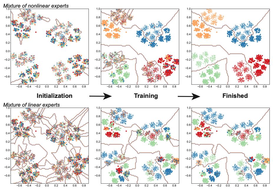
- Another important take-away from this toy experiment is that non-linearity appears to be the key to the success of MoE. Experts with linear activation simply don’t work as well as those with non-linear (cubic in this work) activation.
Mixtral of Experts
- In Mixtral of Experts, the authors perform a routing analysis (i.e., a study on expert specialization) which indicated showed no significant patterns in expert assignment across different topics such as biology, philosophy, or mathematics within The Pile validation dataset, suggesting a mostly syntactic rather than semantic specialization. However, a notable syntactic specialization was observed, where specific tokens in different domains consistently mapped to the same experts, indicating structured syntactic behavior that impacts the model’s training and inference efficiency. Proportion of tokens assigned to each expert on different domains from The Pile dataset for layers 0, 15, and 31. The gray dashed vertical line marks 1/8, i.e. the proportion expected with uniform sampling. Here, they consider experts that are either selected as a first or second choice by the router.

- The figure below from the paper shows repeated consecutive assignments per MoE layer. Repeated assignments occur a lot more often than they would with uniform assignments (materialized by the dashed lines). Patterns are similar across datasets with less repetitions for DM Mathematics.

MoE-LLaVA
- In MoE-LLaVA: Mixture of Experts for Large Vision-Language Models, the authors offer the following findings regarding expert loads and preferences from the provided document, highlighting the dynamic allocation of workloads among experts and their balanced handling of multimodal data.
- Expert Loads:
- The distribution of workloads among experts in the model shows a pattern where different experts take on varying amounts of the total workload depending on the depth of the model layers.
- In the shallower layers (e.g., layers 5-11), experts 2, 3, and 4 primarily collaborate, while expert 1 is more active in the initial layers but gradually withdraws as the layers deepen.
- Expert 3, in particular, dominates the workload from layers 17 to 27, indicating a significant increase in its activation, which suggests that specific experts become more prominent at different depths of the model.
- The figure below from the paper shows a distribution of expert loadings. The discontinuous lines represent a perfectly balanced distribution of tokens among different experts or modalities. The first figure on the left illustrates the workload among experts, while the remaining four figures depict the preferences of experts towards different modalities.
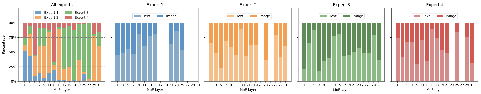
- Expert Preferences:
- Each expert develops preferences for handling certain types of data, such as text or image tokens.
- The routing distributions for text and image modalities are highly similar, indicating that experts do not exhibit a clear preference for any single modality but instead handle both types of data efficiently. This reflects strong multimodal learning capabilities.
- The visualizations of expert preferences demonstrate how text and image tokens are distributed across different experts, revealing that the model maintains a balanced approach in processing these modalities.
- The figure below from the paper shows a distribution of expert loadings. The discontinuous lines represent a perfectly balanced distribution of tokens among different experts or modalities. The first figure on the left illustrates the workload among experts, while the remaining four figures depict the preferences of experts towards different modalities.
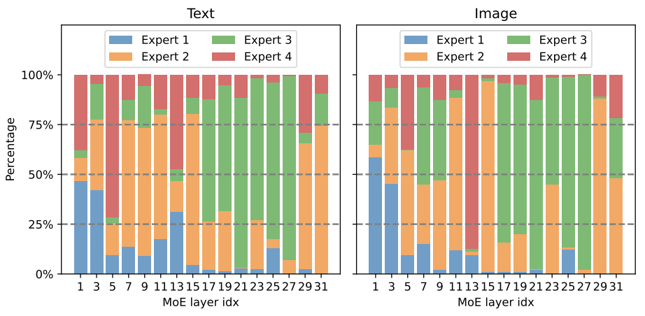
Differentiability of Sparse Routing in Mixture-of-Experts
-
A defining feature of modern Moe architectures is sparse, conditional computation: for each token, only a small subset of experts is activated. This sparsity is typically implemented using a router (or gate) that computes a softmax over expert logits and then applies a hard top-k selection to choose which experts will process the token. At first glance, this hard selection appears incompatible with gradient-based learning because top-k routing is a discrete, non-differentiable operation. However, MoE models remain trainable due to deliberate design choices that introduce biased yet stable gradient estimators.
-
In other words, although sparse MoE routing is not fully differentiable, training remains viable because gradients flow normally through the selected experts, while the router itself is optimized via the underlying soft routing probabilities used before the hard top-k decision. In addition, auxiliary load-balancing losses provide dense optimization signals that encourage effective expert utilization and stabilize training. Together, these mechanisms allow MoE models to benefit from sparse computation without preventing end-to-end learning.
-
This design accepts biased gradients as the cost of conditional computation, enabling MoE architectures to scale to hundreds of billions or trillions of parameters without proportional increases in compute.
-
This section explains how routing is trained despite non-differentiability, and why this approximation works at scale.
Background: Routing Computation Overview
-
Modern sparse MoE layers follow the routing formulation introduced in Outrageously Large Neural Networks: The Sparsely-Gated Mixture-of-Experts Layer by Shazeer et al. (2017) and refined in later systems such as Switch Transformers by Fedus et al. (2021).
-
Let a single input token be represented by a vector
\[x \in \mathbb{R}^{d}\]- where \(d\) is the hidden dimension of the model.
-
The router is a learned linear projection that maps this token representation to a vector of expert logits:
\[z = W_g x\]- where:
- \(W_g \in \mathbb{R}^{N \times d}\) is the router weight matrix, and
- \(N\) is the total number of experts in the MoE layer.
- where:
-
The logit vector \(z = (z_1, z_2, \dots, z_N)\) assigns an unnormalized score \(z_i\) to each expert \(i \in {1, \dots, N}\).
-
These logits are converted into routing probabilities via a softmax:
\[p_i = \frac{\exp(z_i)}{\sum_{j=1}^{N} \exp(z_j)}, \quad i = 1, \dots, N\]- where \(p_i\) denotes the probability of routing token \(x\) to expert \(i\).
-
A sparse selection operator then chooses the indices of the top-\(k\) experts according to these probabilities:
\[\mathcal{E}(x) = \mathrm{TopK}(p, k)\]- where:
- \(k \ll N\) is a small integer (typically \(k = 1\) or \(k = 2\)), and
- \(\mathcal{E}(x) \subset {1, \dots, N}\) is the set of selected expert indices for token \(x\).
- where:
-
Only experts whose indices lie in \(\mathcal{E}(x)\) are executed for this token; all others are skipped.
Non-Differentiability of Top-\(k\) Routing
- The top-\(k\) operator is piecewise constant with respect to the logits \(z\). Infinitesimal perturbations to \(z\) do not change the selected expert set unless the ordering of logits changes. Formally, its gradient is zero almost everywhere:
- As a result, gradients cannot flow through the expert-selection operation itself. This creates an inherent asymmetry between the forward computation graph, which contains discrete routing decisions, and the backward graph, which cannot differentiate through them. Instead, MoE training relies on a partial gradient path that bypasses the discrete selection.
Gradient Flow to Experts
-
Each expert \(E_i\) is a neural network with parameters \(\theta_i\). For experts that are selected (i.e., \(i \in \mathcal{E}(x)\)), gradients propagate normally through their computations.
-
If an expert is not selected for a given token, its output is identically zero and it receives no gradient update:
\[\frac{\partial \mathcal{L}}{\partial \theta_i} = 0 \quad \text{if } i \notin \mathcal{E}(x)\]- where \(\mathcal{L}\) denotes the training loss.
-
This sparse update pattern is intentional and central to MoE scalability. It ensures that both computation and parameter updates scale with \(k\), rather than with the total number of experts \(N\) (GShard by Lepikhin et al. (2020)).
-
Notably, this already breaks forward–backward symmetry: all experts exist in the forward model definition, but only a small subset participates in gradient updates for any given token.h \(k\), not with the total number of experts \(N\) (GShard by Lepikhin et al. (2020)).
Gradient Flow to the Router
-
Although expert selection is discrete, the router still receives gradients through the continuous routing probabilities \(p_i\).
-
Let \(E_i(x)\) denote the output of expert \(i\) applied to token \(x\). The MoE layer output is typically formed as a probability-weighted sum over the selected experts:
- For selected experts, the loss depends smoothly on \(p_i\), which implies:
-
These gradients propagate backward through the softmax into the router parameters \(W_g\). For non-selected experts, both the expert output and its contribution to the loss are zero, and thus they provide no routing gradient signal for that token.
-
This results in a biased gradient estimator: the router is optimized only with respect to experts that were chosen in the forward pass. Despite this bias, training remains stable in large-scale regimes (Scaling Vision with Sparse Mixture of Experts by Riquelme et al. (2021)).
Relation to Straight-Through Estimators
-
This mechanism is closely related to straight-through estimators used in discrete latent variable models (Estimating or Propagating Gradients Through Stochastic Neurons by Bengio et al. (2013)). Conceptually, this creates a deliberately asymmetric computation graph::
- the forward pass uses a hard, discrete decision,
- the backward pass treats routing weights as if they were continuous (and thus assumes a continuous approximation).
- As a result, the router is optimized with respect to a relaxed surrogate objective rather than the exact discrete routing function used at inference time.
- From a symmetry perspective, this explicitly breaks forward–backward equivalence. In a fully symmetric model, the backward pass would compute exact gradients of the same function evaluated in the forward pass. In MoE routing (and straight-through estimators more generally), the backward pass instead computes gradients of a surrogate function.
-
Note that this asymmetry is not unique to MoEs and appears in several other deep learning settings:
-
Examples of symmetric forward–backward flows:
- Standard dense neural networks with continuous activations (e.g., ReLU, GELU), where gradients exactly correspond to the forward computation.
- Soft attention mechanisms, such as Transformer self-attention, where softmax weights are used identically in both forward and backward passes (Attention Is All You Need by Vaswani et al. (2017)).
-
Examples of asymmetric forward–backward flows:
- Straight-through estimators for discrete variables (Bengio et al., 2013).
- Quantization-aware training, where forward passes use quantized weights but backward passes use full-precision gradients (Quantization and Training of Neural Networks for Efficient Integer-Arithmetic-Only Inference by Jacob et al. (2018)).
- Dropout, where units are stochastically removed in the forward pass but gradients are rescaled deterministically (Dropout: A Simple Way to Prevent Neural Networks from Overfitting by Srivastava et al. (2014)).
- REINFORCE-style gradient estimators for stochastic routing or sampling (Simple Statistical Gradient-Following Algorithms for Connectionist Reinforcement Learning by Williams (1992)).
- MoE routing fits squarely into this second category: a controlled, engineered asymmetry that trades exactness for scalability.
-
- While not mathematically exact, this estimator has low variance and scales well in distributed systems, which is critical for large expert counts and trillion-parameter regimes.
Load-Balancing Loss and Dense Router Gradients
-
To prevent routing collapse—where a few experts dominate—modern MoEs introduce an auxiliary load-balancing loss that depends directly on routing probabilities. This idea was introduced in Outrageously Large Neural Networks: The Sparsely-Gated Mixture-of-Experts Layer by Shazeer et al. (2017), and refined in Switch Transformers by Fedus et al. (2021).
-
Let:
- \(f_i\) be the fraction of tokens routed to expert \(i\),
- \(p_i\) be the mean routing probability for expert \(i\).
-
The standard load-balancing loss is:
\[\mathcal{L}_{\text{lb}} = N \sum_{i=1}^{N} f_i p_i\] -
This loss is fully differentiable with respect to the router parameters \(W_g\) and provides gradient signal even for experts that are not selected in the forward pass. Importantly, it partially restores symmetry by introducing a dense, smooth objective that is optimized consistently in both forward statistics and backward gradients. As shown in Switch Transformers by Fedus et al. (2021), this term is critical for maintaining expert utilization and training stability.
Why Biased Gradients Are Acceptable
-
Exact gradients would require evaluating all experts for every token, eliminating the computational advantage of MoEs. Sparse routing therefore trades unbiased gradients for scalability.
-
Empirical evidence across large systems—including GLaM by Du et al. (2022) and MegaBlocks by Gale et al. (2022)—shows that expert specialization reduces gradient interference, biased routing gradients do not prevent convergence, and performance improves as model scale increases.
Implementation
- Credits to the following section go to The AIEdge.
- The Mixture of Experts architecture is relatively straightforward to implement. An implementation that closely aligns with the one found in Mistral 7B is presented below.

Overview
- The architecture, as implemented in the above code, uses a routing mechanism to direct each input token to the most relevant experts. The router, implemented as a linear layer in the
gatevariable, transforms hidden states into logits that are subsequently converted into selection probabilities. These probabilities determine which experts contribute to the output for each token. The final output for each token is a weighted sum of the outputs from the selected experts, ensuring that each part of the input data is processed by the most suitable parts of the network. This method enhances the model’s efficiency and scalability by leveraging specialized networks (experts) only when they are most relevant.
Components
FeedForward Class
- This class defines an individual expert, which is a basic feed-forward network. It consists of three linear layers:
w1andw2transform the input tensor, andw3combines these transformations.
- The
forwardmethod computes the output of this feed-forward network by applying the sequence of transformations and non-linear activations (SiLU, also known as Swish).
MixtureOfExpertsLayer Class
- This class orchestrates the interaction of multiple experts to process the input data.
- Initialization (
__init__):num_experts: Total number of expert networks.n_experts_per_token: Number of experts that should process each token.experts: A list of expert networks.gate: A linear layer that acts as the router, which computes logits (pre-softmax scores) that determine how much each expert contributes to processing each token.
- Forward Pass (
forward):gate_logits: The router outputs logits for each token.weights, selected_experts: Usingtorch.topk, the topn_experts_per_tokenexperts are selected based on the highest logits for each token, indicating which experts are most relevant for each token.weights: Normalized using softmax to convert logits into probabilities indicating the importance of each selected expert’s contribution.out: Initializes an output tensor with zeros, having the same shape as the inputx.- For each expert, the method computes the weighted contribution of the expert’s output to the final output tensor. This is done only for selected experts for each token.
- Initialization (
Expert Choice Routing
-
While traditional MoE models have been integral in scaling transformer-based architectures such as Switch Transformer, GLaM, V-MoE, and FLAN-MoE, they still exhibit challenges that limit their efficiency and fairness in training. One of the most persistent issues is expert under-utilization: certain experts become over-used while others remain under-trained, leading to load imbalance and reduced specialization diversity. These imbalances arise from how routing decisions are made — typically, the gating mechanism chooses the top-\(k\) experts for each token based on compatibility scores, which can lead to overfitting certain experts to specific token distributions. To mitigate this, regularization in the form of a load-balancing auxiliary loss has been introduced to prevent too many examples from being routed to a single or small subset of experts. This loss encourages uniform expert utilization and is defined as:
\[L_{\text{load}} = E \sum_{i=1}^{E} f_i p_i\]- where \(E\) is the number of experts, \(f_i\) represents the fraction of tokens dispatched to expert \(i\), and \(p_i\) is the average gating probability for that expert. This formulation, introduced in Shazeer et al. (2017) and later refined in Zoph et al. (2022), ensures balanced routing and improves overall training stability in sparse MoE architectures.
-
Despite these improvements, token-level routing still tends to produce uneven expert activation and suboptimal hardware efficiency. Because the router assigns experts to tokens independently, it cannot directly control how many tokens each expert processes per batch. This leads to fluctuating expert workloads, unstable gradient updates, and poor Model FLOPs Utilization (MFU) across distributed systems. To overcome this, a new paradigm was proposed that inverts the routing logic—shifting decision-making from tokens to experts.
-
To mitigate this issue, Mixture-of-Experts with Expert Choice Routing by Zhou et al. (2022) at Google introduced Expert Choice (EC) Routing. This method fundamentally rethinks the routing paradigm by reversing the direction of assignment between tokens and experts. Rather than assigning tokens to experts (as in standard MoE routing), EC routing allows experts to choose tokens. This inversion of responsibility has significant implications for training stability, expert specialization, and computational efficiency. By explicitly controlling the number of tokens each expert processes, EC routing achieves inherently balanced workloads, minimizes token overflow, and improves distributed compute utilization.
-
Overall, EC routing represents a paradigm shift in how sparse expert architectures manage routing and specialization. By allowing experts to “choose” their own tokens, it provides superior load balancing, improves specialization, and scales efficiently across distributed systems. This innovation addresses longstanding challenges in traditional MoE systems, offering a robust foundation for the next generation of scalable, efficient, and adaptive large language models.
Core Idea: Reversing the Routing Direction
-
Traditional MoE models employ a token-centric routing strategy. Each token is passed through a gating function that computes a softmax or top-\(k\) score over all available experts, selecting the most relevant ones for processing. Consequently, the gating network determines where each token goes, often leading to congestion among experts that receive high routing scores.
-
In contrast, EC routing adopts an expert-centric routing perspective. Here, the gating network computes a token-to-expert score matrix, where each entry represents how compatible a given token is with a specific expert. Instead of having tokens compete for experts, each expert selects the subset of tokens that it finds most relevant, typically based on the top-\(k\) scoring values. This inversion ensures that every expert processes approximately the same number of tokens, resulting in better load balancing and more uniform expert utilization.
-
The following figure shows the contrast between token-to-expert routing and expert-to-token routing, highlighting how EC ensures balanced load distribution and efficient specialization.
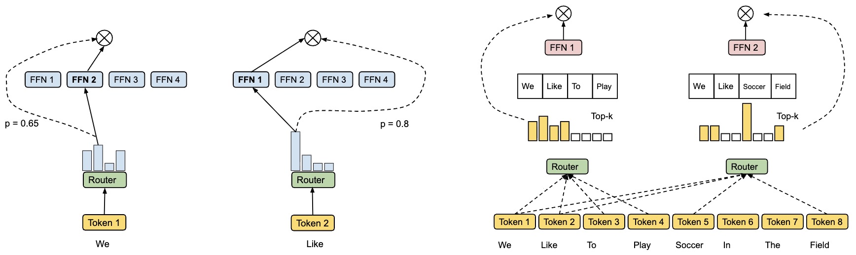
Step-by-Step Workflow of Expert Choice Routing
-
Token-to-Expert Scoring:
-
The EC routing process begins by computing a token-to-expert score matrix, denoted as
\[S \in \mathbb{R}^{T \times E}\]- where \(T\) is the number of tokens and \(E\) is the number of experts.
-
Each element \(S_{t,e}\) represents the relevance or affinity score between token \(t\) and expert \(e\). This score is typically obtained via a linear projection or dot-product similarity in the embedding space.
-
-
Expert Capacity Definition:
- Each expert is assigned a maximum capacity \(C_e\), defined as the number of tokens it can process concurrently.
-
The capacity is determined as:
\[C_e = \text{Capacity Factor} \times \frac{T}{E}\]- where the capacity factor is a hyperparameter controlling the trade-off between load balancing and computational efficiency.
- If the capacity factor is greater than 1, experts may overlap in token assignments, increasing redundancy but also resilience to routing noise.
-
Expert Token Selection (top-\(k\) Selection):
- Each expert independently selects the top-\(k\) tokens from the score matrix that best match its learned specialization.
- This results in an allocation that maximizes compatibility while respecting the expert capacity constraint.
- Mathematically, for expert \(e\):
- where:
- \(\mathcal{T}_e\) denotes the set (or indices) of tokens selected by expert \(e\),
- \(S_{:, e}\) is the column of the score matrix corresponding to expert \(e\),
- and \(C_e\) is the expert’s capacity (i.e., the number of tokens it can process).
-
Permutation and Data Shuffling:
- Once all experts have chosen their tokens, a permutation operation is applied to reorganize the tokens into contiguous blocks assigned to specific experts.
- This step is crucial for computational efficiency, as it enables grouped parallel computation on accelerators (such as GPUs and TPUs) without excessive communication overhead.
- The tokens are then distributed to their respective experts in a format suitable for batched processing.
-
Expert Computation and Output Reassembly:
- Each expert performs its forward computation on its assigned tokens.
- The processed outputs are then passed through an inverse permutation to restore the original token order.
- Finally, the outputs are combined using learned or normalized weights, depending on the aggregation strategy used (e.g., mean pooling, weighted sum).
Advantages of Expert Choice Routing
-
Load Balancing Efficiency: By inverting the routing direction, EC ensures a more uniform distribution of tokens across experts. This eliminates the need for explicit load balancing losses, which are often added to standard MoE architectures to penalize expert overuse.
-
Improved Expert Specialization: Each expert gains control over which tokens it processes, enabling it to develop a clearer and more consistent specialization. This improves convergence and prevents expert collapse (where multiple experts learn redundant behaviors).
-
Reduced Dropping and Padding Overhead: In top-\(k\) routing, when too many tokens are assigned to a popular expert, some must be dropped to maintain computational limits. EC routing’s predefined expert capacity removes the need for token dropping or padding, thereby reducing waste.
-
Enhanced Scalability: EC is more scalable in distributed environments because experts can independently select and process tokens, reducing synchronization costs. This makes EC routing especially advantageous for large-scale systems with thousands of experts.
-
Dynamic Token Prioritization: The EC mechanism naturally prioritizes difficult or ambiguous tokens, since these typically score highly across multiple experts. This adaptive attention to “hard” tokens allows the model to allocate more computational focus where it matters most.
Mathematical Intuition
-
At its core, EC routing optimizes a sparse assignment problem:
\[\max_{A} \sum_{t=1}^{T}\sum_{e=1}^{E} S_{t,e} \cdot A_{t,e}\]-
subject to: \(\sum_{t=1}^{T} A_{t,e} \leq C_e, \quad A_{t,e} \in {0,1}\)
-
where \(A_{t,e}\) represents the binary assignment variable indicating whether token \(t\) is processed by expert \(e\). This optimization ensures each expert operates within its capacity while maximizing global compatibility.
-
-
In practice, this problem is approximated using differentiable top-\(k\) selection and softmax normalization, allowing the routing decisions to remain end-to-end trainable.
Implementation and Integration
- EC routing integrates seamlessly with transformer-based MoE layers, requiring only modifications in the routing subnetwork.
- It is compatible with common deep learning frameworks like TensorFlow and PyTorch, where implementation typically involves:
- Computing token-to-expert scores.
- Applying expert-wise top-\(k\) selection.
- Executing a permutation-based gather-scatter operation.
- The paper demonstrated that EC routing improves perplexity and throughput in language modeling tasks without introducing significant computational overhead, making it an attractive alternative to classic top-\(k\) routing in large language models.
Limitations
-
Increased Routing Complexity: While EC routing balances loads effectively, it introduces additional computational steps during the selection and permutation phases. The construction and manipulation of the token-to-expert score matrix \(S\) can become expensive for large-scale models with millions of tokens or thousands of experts.
-
Communication Overhead: The expert-centric routing process requires collective communication when redistributing token batches among experts, especially in distributed settings. Although the permutation operation is designed for efficiency, it can still create latency in multi-node or multi-GPU environments.
-
Hyperparameter Sensitivity: The performance of EC routing is sensitive to the capacity factor and top-\(k\) settings. Incorrect tuning may lead to token over- or under-assignment, harming both model accuracy and load distribution.
-
Gradient Routing Challenges: Since routing decisions are discrete (due to top-\(k\) selection), gradients must be approximated using continuous relaxations (e.g., Gumbel-softmax or soft top-\(k\)). This approximation can introduce instability during early training or lead to suboptimal expert selection.
-
Specialization Drift: Over the course of training, experts may begin to specialize on overlapping token distributions. Without additional regularization or entropy-based balancing, this overlap can reduce diversity across experts, negating some of the benefits of distributed specialization.
-
Implementation Complexity in Practice: Integrating EC routing into large-scale frameworks requires careful engineering of parallel and distributed computation primitives. Many current deep learning libraries provide limited native support for expert-centric communication patterns, necessitating custom kernels or frameworks (such as GSPMD or DeepSpeed-MoE).
Mixture-of-Experts Beyond MLP Layers
Motivation
- Traditionally, MoE layers have been integrated primarily into the feed-forward (MLP) blocks of transformer architectures. This design exploits conditional computation to scale model parameters without proportional increases in compute. However, limiting MoE to the MLP layers underutilizes its potential — transformer blocks also include attention mechanisms, connectors, and modality-specific encoders that can benefit from conditional sparsity.
-
The evolution of MoE beyond MLP layers marks a significant turning point in scalable neural network design:
- MoE is no longer confined to feed-forward modules—it now extends to attention, connectors, and encoders.
- These expansions enable semantic specialization across modalities, allowing experts to capture structured relationships in vision-language tasks.
- Works like CuMo, V-MoE, LIMoE, and Uni-MoE collectively illustrate this trend, providing both theoretical justification and empirical success.
-
Recent works explore expanding MoE principles to these non-MLP components. The motivation is twofold:
- Representation diversity: Different modalities (text, vision, audio) or architectural components (attention heads, encoders) require distinct forms of specialization.
- Compute efficiency: Selectively activating experts across broader network regions allows models to scale without saturating GPU memory or compute budgets.
MoE in Attention Layers
-
A growing body of work investigates extending MoE to attention sublayers, which traditionally remain dense even in sparse architectures. The MoA (Mixture-of-Attention) concept replaces the single self-attention mechanism with a set of attention experts, each specializing in different token dependencies or context types.
-
Formally, for a token sequence \(X \in \mathbb{R}^{N \times d}\), instead of computing one attention map:
-
MoA introduces a router that assigns tokens to one or more attention experts:
\[\text{MoA}(X) = \sum_{i=1}^E g_i(X) , \text{Attn}_i(X),\]- where \(g_i(X)\) are routing weights (soft or hard) for each attention expert \(i\).
-
This approach, explored in works like MoA-Transformer (Zhao et al., 2024), enables diverse attention patterns — for example, one expert may specialize in short-range syntactic dependencies while another captures long-range semantic relations. Such routing-driven diversity has shown improvements in language modeling perplexity and multimodal reasoning tasks.
MoE in Modality Encoders and Connectors
Vision Encoders
-
In multimodal systems, the vision backbone represents a significant compute bottleneck. CuMo by Li et al. (2024) introduces Co-Upcycled MoE (CuMo), which integrates sparse Top-K MoE blocks into both the vision encoder and the MLP connector of multimodal LLMs. Each MoE expert in the vision encoder is initialized (“upcycled”) from a pre-trained dense MLP block, maintaining stability while enhancing scalability.
-
Their training pipeline involves three stages — pre-training, pre-finetuning, and co-upcycled MoE integration — ensuring that the sparse experts inherit useful priors before specialization. This co-upcycling strategy achieves strong results on benchmarks like MMBench, GQA, and MMMU, outperforming models such as LLaVA-NeXT and Mini-Gemini.
-
Mathematically, the CuMo architecture replaces a dense vision-encoder layer:
-
… with a sparse variant:
\[Y = \sum_{i=1}^{K} g_i(X) \cdot \text{Expert}_i(X),\]- where the router selects top-\(K\) experts and enforces balanced usage through auxiliary load-balancing losses.
Connectors and Adapters
- The MLP connectors between modalities also benefit from expert routing. CuMo’s design integrates MoE into these connectors to improve the alignment between visual and textual embeddings. Similarly, MoE-LLaVA (Zhang et al., 2023) introduces expert-specialized adapters within multimodal connectors, achieving substantial improvements in instruction-following and grounding tasks without increasing inference cost.
Cross-Modal and Multimodal MoE
-
Beyond individual encoders, multimodal frameworks have begun using MoE as a cross-modal fusion mechanism. For instance, LIMoE: Multimodal Contrastive Learning with LIMoE: the Language-Image Mixture of Experts by Mustafa et al. (2022) extends MoE into CLIP-style architectures by inserting expert layers in both visual and text towers. Each expert specializes in a specific modality distribution or visual concept. This structure significantly improves zero-shot image classification and text-image retrieval performance while maintaining computational efficiency.
-
Similarly, V-MoE: Scaling Vision with Sparse Mixture of Experts by Riquelme et al. (2021) demonstrates that replacing dense MLP layers with sparse experts in vision transformers leads to comparable accuracy with half the compute. These advances confirm that MoE designs are not only scalable but also modality-adaptive, enabling cross-domain generalization.
Joint MoE Architectures
-
Recent multimodal systems explore joint MoE formulations where both the attention and feed-forward layers are expert-based, creating a hierarchical sparsity pattern. For example:
- Union of Experts: Adapting Hierarchical Routing to Equivalently Decomposed Transformer by Yang et al. (2025) proposes hierarchical routing, where global experts manage modality interaction, while local experts specialize in intra-modal refinement.
- Uni-MoE: Scaling Unified Multimodal LLMs with Mixture of Experts by Li et al. (2024) uses shared routing across text and vision experts, enabling parameter sharing and reducing routing entropy.
- HC-SMoE: Retraining-Free Merging of Sparse MoE via Hierarchical Clustering by Chen et al. (2025) introduces a hierarchical clustering approach for sparsely activated MoE—merging similar experts without retraining, which aligns naturally with hierarchical expert organization.
-
These architectures embody a shift toward multi-granular expert specialization, where different experts handle distinct facets of reasoning—spatial, textual, semantic, or modality-specific.
Theoretical and Practical Implications
-
Expanding MoE beyond MLP layers introduces new challenges and opportunities:
- Routing complexity increases, requiring hierarchical or differentiable router designs to maintain efficiency.
- Load balancing becomes multidimensional—covering both tokens and modalities.
- Transferability improves, as experts pre-trained on one modality can often generalize to others under joint training.
-
Formally, the total computation cost of multimodal MoE can be expressed as:
\[C_{\text{MoE-total}} = \sum_{l=1}^{L} K_l \cdot C_{\text{expert}}^{(l)},\]
Beyond Token-based Routing: Structural and Hierarchical Routing Paradigms
Overview
- Conventional MoE frameworks treated each token as an independent routing unit, sending it to the most compatible expert(s) based on gating scores. While effective, this token-wise routing neglects structural relationships — such as inter-token dependencies, syntactic grouping, or semantic coherence.
- As models grow in size and context windows expand, such isolated routing becomes increasingly inefficient and unstable.
- To address this, researchers have begun developing structure-aware and hierarchical routing paradigms that capture higher-order relationships — between tokens, concepts, or entire regions of input. These new paradigms leverage cluster formation, graph structures, and expert hierarchies to promote both interpretability and computational efficiency.
- This evolution is well represented by works such as On the Benefits of Learning to Route in Mixture-of-Experts Models by Dikkala et al. (2023), Mixture-of-Experts with Expert Choice Routing by Zhou et al. (2022), Improving Routing in Sparse Mixture of Experts with Graph of Tokens by Nguyen et al. (2025), and AdaMoE: Token-Adaptive Routing with Null Experts for Mixture-of-Experts Language Models by Zeng et al. (2024). Collectively, these works demonstrate a decisive shift from independent token-level decisions to concept- and structure-driven routing in large-scale MoE architectures.
- The evolution from token-wise to structure- and hierarchy-aware routing represents a pivotal shift in Mixture-of-Experts research. By leveraging clusters, attention graphs, and adaptive routing, these systems now learn to organize knowledge semantically, rather than relying purely on statistical matching.
Motivation
-
The motivation for structural and hierarchical routing in MoE models stems from the growing recognition that token-level routing—though effective for sparsity and efficiency—fails to capture the deeper semantic, relational, and structural patterns inherent in data. As model capacity scales, how tokens are routed becomes as important as which experts they reach.
-
Semantic and structural coherence: Tokens or inputs that share semantic or syntactic functions (e.g., all math-related symbols, or tokens in a dialogue segment) should ideally be processed by the same or related experts. This coherence allows experts to specialize more deeply in conceptual domains rather than handling disjoint, unrelated inputs.
-
Avoiding token fragmentation: Independent routing often fragments semantically related tokens across multiple experts, leading to unstable learning dynamics. This fragmentation reduces expert specialization and hinders generalization, as experts receive highly diverse or noisy data distributions. Works such as On the Benefits of Learning to Route in Mixture-of-Experts Models by Dikkala et al. (2023) demonstrate that structured grouping of tokens yields more robust representations.
-
Capturing inter-token dependencies: Incorporating token relationships through similarity metrics, attention maps, or graph structures—as in Improving Routing in Sparse Mixture of Experts with Graph of Tokens by Nguyen et al. (2025)—enables routing decisions that are context-aware rather than independent. This reduces routing “fluctuations” and improves specialization stability across training.
-
Efficiency and interpretability: Structured routing also minimizes redundant computation by reducing frequent expert switching and unnecessary dispatch operations. Grouped tokens routed together lead to fewer communication overheads and more interpretable routing maps (e.g., Expert A handles reasoning tokens, Expert B processes visual descriptions). Such interpretability has been observed in architectures like Mixture-of-Experts with Expert Choice Routing by Zhou et al. (2022), where experts self-organize around coherent semantic patterns.
-
Scalability and balance: Hierarchical and cluster-aware routing promotes scalability by balancing loads across groups of experts instead of individual experts. It ensures that no single expert is overwhelmed, while semantically aligned experts collaborate efficiently under shared routing hierarchies, as seen in hierarchical approaches like Sparse-Transformer++ by Xu et al. (2024).
-
-
In essence, the motivation behind moving beyond token-wise routing is to align computational structure with semantic structure — enabling experts to mirror the inherent organization of language, vision, or multimodal data. This paradigm shift transforms routing from a purely statistical operation into a semantically informed decision process, laying the foundation for more interpretable, efficient, and stable sparse architectures.
Structural and Concept-Aware Routing
- Structural routing extends the traditional MoE paradigm by recognizing that tokens in natural language or multimodal data are rarely independent. Words in a phrase, patches in an image, or frames in a video exhibit strong contextual dependencies.
Clustering-Based Routing
-
In On the Benefits of Learning to Route in Mixture-of-Experts Models by Dikkala et al. (2023), the gating network learns implicit clusters of tokens with similar semantics. The router automatically assigns tokens from the same latent group to a shared expert, effectively discovering conceptual clusters without explicit supervision.
-
Empirically, such clustering reduces expert fragmentation and stabilizes training, as related tokens are processed together. The clustering tendency can be formalized as minimizing intra-cluster variance:
\[\mathcal{L}_{\text{cluster}} = \sum_{i=1}^{E} \sum_{x \in \mathcal{C}_i} | f(x) - \mu_i |^2\]- where \(f(x)\) is the router embedding of token \(x\), \(\mu_i\) is the centroid for expert \(i\), and \(\mathcal{C}_i\) is the token cluster routed to expert \(i\).
Concept-Driven Specialization
- By associating experts with consistent conceptual regions of input space (e.g., math symbols, logical reasoning, or dialogue tone), models develop deeper specialization and interpretability. This emergent conceptual routing has been observed in both Switch Transformers and follow-up works such as Expert Choice Routing, which show that experts often converge toward semantic roles without explicit supervision.
Hierarchical Routing Architectures
- Hierarchical routing introduces a multi-level expert organization where gating occurs at multiple granularities — e.g., clusters of experts managed by super-experts or global routers.
Multi-Level Expert Graphs
- In Sparse-Transformer++ by Xu et al. (2024), routing is decomposed into two stages:
- A global router selects an expert group based on coarse semantic attributes.
- A local router within that group selects the final expert(s) based on finer token-specific features.
-
This hierarchical structure is mathematically defined as:
\[g_i(x) = g_{\text{global}}(x) \cdot g_{\text{local}}^{(i)}(x)\]- where \(g_{\text{global}}\) governs coarse-grained selection across groups and \(g_{\text{local}}^{(i)}\) refines the choice within group \(i\).
-
This two-level design improves routing efficiency (fewer gating operations per token) and enhances expert stability, as related experts co-evolve under shared global context.
Hierarchical Load Balancing
-
Hierarchical models require new balancing strategies to prevent group-level saturation. Load can be defined recursively:
\[\text{Load}_{\text{group}_j} = \sum_{i \in \text{group}_j} f_i P_i\]- where \(f_i\) and \(P_i\) are the fraction and probability for expert \(i\) respectively (as defined in Switch Transformer). Balancing at both the expert and group levels prevents bottlenecks and ensures smooth scaling to hundreds or thousands of experts.
Graph- and Attention-Based Routing
-
Moving beyond pairwise similarity, recent work by Nguyen et al. (2025) introduces a Graph of Tokens (GoT) framework, in which routing is modeled as a message-passing process. Each token becomes a node, and edges encode semantic or attention-based affinities.
-
The routing distribution is then computed via a graph propagation function:
\(p_i(x) = \text{softmax}!\left( \frac{1}{|\mathcal{N}(x)|} \sum_{x' \in \mathcal{N}(x)} w(x, x') , \phi(x') \right),\)
- where \(w(x, x')\) measures similarity between tokens and \(\phi(x')\) represents their local routing states.
-
This framework promotes relational coherence, routing similar tokens jointly and significantly improving generalization in sparse MoE models.
Adaptive and Token-Group Routing
-
Beyond static token clusters, models such as AdaMoE introduce dynamic token grouping. Each token adaptively decides:
- how many experts to engage, and
- whether to skip computation entirely (via null experts).
-
Formally, for token \(x\):
\[\text{Routing}(x) = \sum_{i \in \mathcal{S}(x)} g_i(x) \cdot \text{Expert}_i(x),\]- where \(\mathcal{S}(x)\) is a dynamically determined set of active experts, possibly empty. This allows the model to modulate computation intensity based on token complexity, improving efficiency without degrading accuracy.
Benefits, Limitations, and Open Questions
Benefits
- Improved specialization: Experts trained on coherent semantic groups learn deeper and more transferable representations.
- Stable routing dynamics: Structured gating mitigates routing noise, as observed in Improving Routing in Sparse Mixture of Experts with Graph of Tokens by Nguyen et al. (2025).
- Interpretability: Experts increasingly correspond to identifiable domains or concepts (e.g., reasoning, syntax).
- Efficiency gains: Clustering reduces redundant expert activations and routing overhead.
Limitations
- Latent specialization: Conceptual groupings are emergent rather than explicitly controlled.
- Computational overhead: Computing token-token similarity or maintaining graphs adds cost.
- Load balancing: Balancing across groups of experts or clusters remains non-trivial.
- Domain shift sensitivity: Clusters may drift under distributional changes.
Open Questions
- Can we explicitly label experts by domain or concept during training?
- How does concept-aware routing scale to trillion-parameter MoEs?
- What are the best metrics to evaluate semantic coherence in expert routing?
- Can routing be made hierarchically differentiable, allowing backpropagation through cluster assignments?
- How does routing hierarchy affect transfer and continual learning?
Expert Parallelism
Overview
-
Expert Parallelism (EP) refers to a model-parallelism strategy in which the distinct expert subnetworks are distributed across different devices (e.g., GPUs) rather than being replicated or tensor-sharded in the usual way. For high-level context: a typical MoE model comprises a gate (router) network that selects a subset of expert subnetworks (e.g., feed-forward layers) to process each token or input. By activating only a few experts per input, one gains a parameter-efficient model that uses a high total parameter count while keeping FLOPs somewhat restricted. Please refer Wikipedia: Mixture of Experts for further background.
-
EP enables leveraging that sparsity in a distributed training/inference setup: each device holds one (or more) full experts (rather than parts of all experts), and tokens are routed to the devices which hold the selected experts. This contrasts with tensor parallelism (splitting weights of a layer across devices) or pipeline parallelism (splitting layers across stages). EP is a type of model parallelism that distributes experts of an MoE across GPUs; unlike other model-parallel techniques, EP is applied to only the expert layers thus does not impact the parallel mapping of the rest of layers. The user guide for NVIDIA NeMo Framework offers further details on the specific steps to carry out EP.
-
In this section, we will lay out what EP is (definition and motivation), how it fits into the taxonomy of parallelism approaches (data, tensor, pipeline, expert), and the high-level benefits and trade-offs. In subsequent sections, we will dive deeper into implementation details, communication patterns, load-balancing issues, and scaling analysis.
Definition and taxonomy
What is expert parallelism?
-
More formally, consider a MoE layer in a neural network. Suppose there are \(E\) experts (sub-networks) in that layer, labeled \(f_1, f_2, \dots, f_E\). An input token (or vector) \(x\) is routed via a gating function \(g(x)\) which selects a subset of experts (often the top-\(k\) scoring experts) to process \(x\). In a standard MoE scenario, one writes:
\[y = \sum_{i = 1}^{E} w_i(x) f_i(x)\]- where \(w_i(x)\) is non-zero only for a small subset of experts. (cf. Learning Factored Representations in a Deep Mixture of Experts by Eigen et al. (2013).)
-
In EP, the distribution strategy is: each expert \(f_i\) is assigned to a particular device (or a group of devices). Thus device \(d_j\) might host a subset of experts \(E_j \subseteq {1,2,\dots,E}\). Then when tokens are routed, one must send the token data to the device(s) hosting the selected experts, compute \(f_i(x)\), and then collect the outputs. This allows each device to perform full expert forward/backward passes for the ones it hosts.
Positioning among parallelism strategies
-
It helps to place EP alongside other common paradigms:
- Data parallelism (DP): All devices hold a full copy of the model; different devices process different batches of data.
- Tensor parallelism (TP): A given layer’s weights are partitioned (e.g., split across columns/rows) across devices; each device computes a portion of that layer’s operation, and then results are combined. (See e.g., Paradigms of Parallelism by Colossal-AI.)
- Pipeline parallelism (PP): Different layers are assigned to different devices; for a forward pass, tokens/properties are passed through the pipeline of devices.
- Expert parallelism (EP): A subtype of model parallelism where complete experts (sub-networks) are distributed, rather than splitting weights of a single expert. For example, the DeepSpeed MoE implementation tutorial states: “The GPUs (or ranks) participating in an expert-parallel group of size
ep_sizewill distribute the total number of experts specified by the layer.”
-
Thus EP can be thought of as a specialization of model parallelism particular to MoE architectures; in fact, many large MoE systems use a hybrid parallelism combining DP + TP + EP (and sometimes PP) to scale in three dimensions (data, tensor weights, expert sub-networks). See Section 4 below for more on this.
Why expert parallelism matters
-
The rationale for EP is multi-fold:
- Parameter scale: MoE models allow huge parameter counts (e.g., tens of billions) while only activating a small fraction per input. EP allows distributing those many parameters across devices, so no single device must hold all of them. For example, the blog about training MoEs at scale with PyTorch notes: “As models scale to larger sizes and fail to fit on a single GPU, we require more advanced forms of parallelism. EP is a form of model parallelism where we place different experts on different GPUs for better performance.”
- FLOP/activation efficiency: By routing only to a small subset of experts, each input performs fewer FLOPs than activating all experts. EP then ensures that the computational workload is distributed across devices and each device executes reasonably large matrix multiplications (better GPU utilization) rather than many tiny ones.
- Memory efficiency: Because not all experts are active for each input, and each device holds only part of the expert set, the peak memory footprint per device is reduced compared to naive replication of all experts.
- Scalability: EP enables scaling the number of experts \(E\) and total model capacity without linearly increasing the per-token compute budget (assuming only a small number of experts active per token). This helps achieve almost constant cost per token with increasing parameter counts.
Device Partitioning, Token Routing, and Communication Mechanics
- EP provides an elegant mechanism to map sparsely activated experts onto distributed hardware while preserving high model capacity. It relies on efficient all-to-all communication and balanced routing to ensure scalability. Modern frameworks optimize these aspects through load-balancing losses, fused collectives, and hybrid parallel designs.
Conceptual overview
-
EP works by partitioning experts across multiple devices and dynamically routing token representations to the appropriate devices that host the selected experts. Each expert is a self-contained sub-network—typically a feed-forward block within a Transformer layer. During a forward pass, each input token is assigned to one or more experts according to the routing probabilities produced by the gating network (often a softmax-normalized linear projection of the token embeddings).
-
Formally, let \(E\) denote the total number of experts and \(D\) the number of available devices. We define a device-to-expert mapping function
- such that expert \(e_i\) resides on device \(\phi(i)\). Each token \(x_j\) is routed to a subset of experts \(S_j = {e_{j1}, \dots, e_{jk}}\) with corresponding gating weights \(w_{j1}, \dots, w_{jk}\). The forward output is computed as
-
where \(f_{e_i}\) is the expert network’s transformation (typically a two-layer MLP with activation).
-
This dynamic routing implies an all-to-all communication pattern between devices: tokens assigned to experts on remote devices must be sent there, processed, and returned. The design challenge in EP is therefore to minimize communication overhead and maintain load balance so that each device receives a roughly equal number of tokens.
Communication flow
- The canonical all-to-all routing pipeline follows these steps (as used in systems like GShard by Lepikhin et al. (2020), Switch Transformer by Fedus et al. (2021), and DeepSpeed-MoE):
- Token grouping: For each token, the gate determines its top-\(k\) experts. Tokens are grouped by destination expert.
- All-to-all dispatch: Each device sends token embeddings to the devices hosting the relevant experts. This step dominates communication cost.
- Local expert computation: Each device executes its local experts on the received tokens, producing expert outputs.
- All-to-all gather: Expert outputs are sent back to the originating devices.
- Combination: Each token’s outputs are recombined (weighted by its gating weights \(w_{ji}\)) to produce the final MoE layer output.
- In modern frameworks, both dispatch and gather operations are implemented using highly optimized collective primitives such as NCCL all-to-all or fused CUDA kernels. The cost is largely proportional to \(O(B \times H / D)\) where \(B\) is batch size and \(H\) hidden dimension, assuming uniform routing.
Load balancing across experts
-
Because routing is probabilistic, some experts may receive more tokens than others. Uneven token-to-expert assignment creates two performance issues:
- Underutilization: Idle GPUs waste compute capacity when few tokens are routed to their experts.
- Stragglers: Overloaded experts increase step time, since synchronization waits for all devices to finish processing.
-
To mitigate this, MoE systems introduce an auxiliary load-balancing loss—for instance the formulation from Switch Transformer:
-
where \(f_i\) is the fraction of tokens routed to expert \(i\), \(P_i\) is the average routing probability for expert \(i\), and \(\lambda\) is a weighting coefficient. Minimizing this term encourages uniform token distribution, preventing collapse of routing onto a few experts. (Also discussed in Towards Understanding Mixture of Experts in Deep Learning by Chen et al. (2022).)
-
Another complementary approach is Expert Choice Routing (Mixture of Experts with Expert Choice Routing by Zhou et al. (2022)), which inverts the routing direction: each expert selects which tokens to process based on its capacity and affinity, improving balance and locality. A detailed discourse on capacity factor is available in the Expert Choice Routing section.
Communication–computation trade-off
- The performance of EP is determined by the ratio of communication time \(t_{\text{comm}}\) to computation time \(t_{\text{comp}}\). Let \(T\) denote the total number of tokens per batch, \(k\) the number of selected experts per token, \(E\) the number of experts, and \(D\) the number of devices. A simplified cost model can be written as
-
where BW is interconnect bandwidth and TFLOPs the compute throughput per device. Efficient systems therefore aim to (i) minimize \(k\), (ii) overlap communication with compute, and (iii) route tokens so that most stay local (intra-node routing).
-
State-of-the-art frameworks such as Megablocks by Gale et al. (2022) and DeepSpeed-MoE adopt block-sparse layouts and fused all-to-all operations to reach near-linear scaling up to hundreds of GPUs.
Hybrid parallel strategies
-
Because EP only distributes MoE layers, production-grade systems often combine it with other parallelism types:
- Data + EP: Each data-parallel replica holds a different subset of experts, reducing memory cost per GPU while maintaining large global batch size.
- Tensor + EP: Inside each expert, weight matrices may still be tensor-parallelized to fit very large hidden dimensions (e.g., in GLaM by Du et al. (2021)).
- Pipeline + EP: Different layers are placed in pipeline stages while MoE experts are spread within each stage (see Pathways by Barham et al. (2022)).
-
These hybrid designs achieve efficient scaling across thousands of accelerators. For instance, Google’s Pathways system demonstrated scaling of MoE models to trillions of parameters using combinations of data, tensor, and EP.
Capacity Management and Adaptive Token-to-Expert Assignment
Motivation
-
In expert-parallel architectures, each expert has a finite processing capacity per forward pass—determined by GPU memory, batch size, and routing limits. When the gate assigns too many tokens to a single expert, that expert’s device may run out of memory or cause latency spikes due to queue imbalance. Therefore, MoE systems impose an explicit capacity constraint on each expert, which regulates the number of tokens it can process per batch.
-
Capacity management is a crucial aspect of EP, ensuring that per-device workloads remain balanced and memory-safe. Adaptive gating, dynamic capacity scaling, and fused dispatch kernels collectively stabilize large-scale MoE training. These optimizations make trillion-parameter MoE models—such as GLaM, Switch Transformer, and Pathways—feasible on practical clusters.
-
Let \(C\) denote the maximum number of tokens an expert can handle in one pass. If the total number of tokens routed to expert \(e_i\) is \(T_i > C\), the system must either drop or reassign the overflow tokens.
-
This issue was first highlighted in Switch Transformer by Fedus et al. (2021), which introduced the “expert capacity factor” to control token routing loads and ensure training stability.
Capacity factor and token dropping
- Each expert’s capacity is usually computed as:
-
where:
- \(T\) is the total number of tokens in the batch,
- \(k\) is the number of experts each token is routed to (typically 1 or 2),
- \(E\) is the total number of experts, and
- \(\alpha\) is the capacity factor (a scalar > 1 to provide buffer capacity).
-
If the assigned tokens \(T_i > C\), excess tokens are handled by one of several strategies:
- Dropping: The overflow tokens are ignored (their gradient is set to zero). This is simple but may slightly degrade accuracy.
- Random reassignment: Overflow tokens are redirected to underutilized experts.
- Padding/truncation: Tokens beyond capacity are truncated but still contribute partially to load statistics.
-
For instance, the GLaM model by Du et al. (2021) used top-2 gating with load balancing and a fixed capacity factor \(\alpha = 1.25\), ensuring that only ~1% of tokens were dropped at scale.
-
These mechanisms strike a balance between training efficiency, load uniformity, and memory constraints.
-
A detailed discourse on capacity factor is available in the Expert Capacity and Capacity Factor section.
Dynamic capacity adjustment
-
Recent MoE frameworks implement adaptive capacity management, where each expert’s capacity is automatically tuned based on observed routing statistics. For example:
- BASE Layers by Lewis et al. (2021) introduced a layer-wise balancing mechanism where capacity allocation is proportional to historical token loads.
- Tutel (Microsoft Research, 2022) dynamically adjusts expert buffer sizes and uses token sorting to reduce dispatch irregularity.
- DeepSpeed-MoE implements adaptive “capacity-aware all-to-all” communication, skipping empty slots and compressing routing payloads for communication efficiency.
-
The core idea is that if certain experts consistently receive fewer tokens, their capacity can be reduced to free resources for heavily used experts—improving both compute utilization and memory footprint.
Routing strategies and adaptive gating
-
The gate network itself can evolve to improve token assignment. Beyond static top-k routing, advanced strategies include:
- Noisy Top-k Gating (GShard by Lepikhin et al., 2020): Adds Gaussian noise to logits before selecting experts to encourage exploration and load balance.
- Load-Balanced Routing (Switch Transformer): Adds auxiliary loss to penalize expert imbalance.
- Expert Choice Routing (Zhou et al., 2022): Each expert independently selects a subset of tokens it wants to process, improving locality.
- Hash-based Routing (Hash Layers by Roller et al., 2021): Uses consistent hashing to deterministically map tokens to experts, removing the gate’s learned component for predictability and speed.
- Soft MoE (Soft MoE by Shen et al., 2021): Performs continuous, differentiable routing where all experts contribute but are weighted softly, removing discontinuities in gating gradients.
-
These routing methods trade off between expressiveness (learned gates) and efficiency (deterministic or sparse routing). Hybrid approaches can even mix them layer-wise in the same model.
Capacity overflow analysis
- Consider the case of top-1 gating. Let \(p_i\) denote the probability that a token is assigned to expert \(i\), so \(\sum_i p_i = 1\). If routing is stochastic but independent across tokens, the number of tokens assigned to expert \(i\) follows a Binomial distribution:
- … and the expected number of overflows is:
-
Balancing losses attempt to make \(p_i \approx 1/E\), thus minimizing expected overflow. In practice, systems choose \(\alpha \in [1.0, 1.5]\) for stable training with minimal drops.
-
Empirical results from Switch Transformer showed that for large-scale models with \(E=2048\) experts, setting \(\alpha = 1.25\) yielded optimal trade-offs between speed and accuracy, allowing >99% tokens to be processed successfully per step.
Example: capacity-aware token routing
-
In modern implementations such as NVIDIA Megatron-Core MoE, the routing kernel incorporates capacity-aware padding. Tokens are packed into contiguous buffers, respecting expert capacity, and an optimized fused kernel performs:
- Token sorting by expert ID
- Capacity clipping
- Memory offset computation
- Expert batch matmul in fused CUDA kernel
- Gather back using prefix-sum indices
-
This design removes Python-level overhead and maintains consistent throughput even under non-uniform routing patterns. Benchmarks show that expert-parallel MoE with fused dispatch achieves near-linear scaling to 512 GPUs.
Limitations
-
MoE architectures enable dramatic increases in model capacity with only a modest rise in computation by relying on sparse, conditional activation of parameters. This design makes them highly attractive for large-scale training, where they can achieve impressive performance and theoretical efficiency without proportionally increasing compute costs.
-
However, the same architectural choices that make MoEs powerful also introduce fundamental limitations that complicate training stability, inference efficiency, and real-world deployment. Because computation is sparse but parameters are not, MoE models typically require the full expert set to reside in memory, even though only a small fraction is active for any given input. This disconnect creates significant challenges around memory pressure, system complexity, and deployment flexibility.
-
While MoEs excel during training, inference-time memory residency emerges as the dominant practical bottleneck. Until memory usage can scale with active computation rather than total parameter count, MoE architectures will remain difficult to deploy broadly—despite their compelling efficiency gains on paper and their success at scaling model capacity.
Inference-Time Memory Residency and VRAM Requirements (Primary Limitation)
-
The single largest barrier to the adoption and deployment of MoE models is their inference-time memory footprint, which scales with total model capacity rather than with active computation.
-
Despite sparse activation, all experts must remain resident in memory during inference:
- Each expert is a distinct parameterized network.
- Routing decisions are dynamic, token-level, and input-dependent.
- It is generally impossible to know ahead of time which experts will be activated for a given request.
-
As a result, inference systems must load and keep every expert in GPU (or accelerator) memory to guarantee low-latency access. This fundamentally breaks the intuitive expectation that sparse computation should imply sparse memory usage.
-
Key consequences at inference time:
-
Memory scales with total parameters, not active parameters: Even if only 1–2 experts are used per token, VRAM usage reflects the full MoE layer. This makes MoEs memory-bound rather than compute-bound at inference.
-
Severe constraints on batch size and throughput: High VRAM pressure limits how many concurrent requests can be served. Increasing batch size often becomes impossible long before compute is saturated.
-
High cold-start and autoscaling cost: All experts must be loaded before serving, leading to slow startup times and expensive autoscaling in production systems.
-
Poor memory amortization across requests: Different inputs activate different experts, preventing aggressive caching or eviction strategies. Even “simple” inputs require the entire expert pool to be present.
-
Multi-layer amplification: Modern MoEs typically place experts in multiple transformer layers. Memory usage compounds across layers, making deep MoEs especially difficult to deploy.
-
-
Concrete examples illustrate the severity of this constraint:
- Switch Transformer and GLaM required full expert residency on high-memory TPU pods.
- Large open MoEs such as Mixtral-8×7B must keep all experts loaded, consuming tens of gigabytes of VRAM per device—even though only a fraction are active per token.
-
To serve MoEs at scale, practitioners must choose between:
- Very high-memory accelerators (80–120 GB GPUs, large TPU slices), or
- Expert offloading to CPU/NVMe, which introduces substantial latency and negates many of MoE’s inference advantages.
-
Despite ongoing work on expert offloading, demand paging, pruning, and quantization, MoE architectures fundamentally lower compute per token while leaving inference-time memory requirements tied to the full model size.
-
In practice, this makes MoEs significantly harder—and often more expensive—to deploy than dense models, especially in latency-sensitive or cost-constrained environments.
Training Instability and Load Imbalance
-
MoE models are inherently prone to uneven expert utilization, where a small subset of experts receives the majority of tokens while others remain underused or idle. This load imbalance leads to unstable optimization, undertrained experts, and degraded generalization.
- The issue was first identified in Sparsely-Gated MoE, which introduced a load-balancing loss to encourage uniform routing.
- Later work such as Expert Choice Routing reversed the routing direction, allowing experts to select tokens in an attempt to improve utilization.
- Despite these advances, perfect balance remains elusive—especially at scale.
-
Imbalance has several compounding effects:
- Experts that receive fewer tokens learn more slowly or not at all.
- Overused experts experience higher gradient variance and saturation.
- The system becomes fragile to routing noise, increasing the risk of expert collapse.
-
In large distributed setups, even small routing skews can significantly slow convergence and reduce effective capacity.
Communication Overhead and Hardware Dependency
-
Although MoEs are computationally sparse, they are communication-heavy.
-
During training (and often inference), tokens must be dynamically routed to experts that may reside on different devices. This introduces expensive all-to-all communication patterns:
- Token activations must be exchanged across devices.
- Synchronization barriers become frequent.
- Network bandwidth, not FLOPs, often becomes the bottleneck.
-
Systems such as GShard and Switch Transformer rely on:
- custom kernels,
- carefully engineered all-to-all collectives,
- extremely high-bandwidth interconnects (TPU mesh, NVSwitch).
-
On commodity GPU clusters, communication overhead can dominate total runtime, eroding or even reversing the theoretical efficiency gains of sparsity. This makes MoE training and inference feasible primarily on hyperscale infrastructure, limiting accessibility.
-
In short: MoEs trade dense compute for sparse compute—but replace it with dense communication.
Routing Complexity and Gradient Fragmentation
-
The routing mechanism that selects experts introduces both algorithmic and optimization complexity.
- Routing decisions are typically based on top-\(k\) selection over expert logits.
- These decisions are discrete and non-differentiable.
- Approximations such as soft routing, stochastic gates, or straight-through estimators are required.
-
These approximations introduce noise and instability:
- Small changes in router parameters can dramatically change expert assignments.
- Tokens may be misrouted, slowing expert specialization.
- Gradients become unevenly distributed across experts.
-
This leads to gradient fragmentation, where some experts receive dense, stable gradients, while others receive sparse, noisy, or delayed updates.
-
Fragmentation makes optimization more brittle and increases sensitivity to hyperparameters such as learning rate, routing temperature, and auxiliary loss weights.
Underutilization of Model Capacity
-
Although MoEs contain enormous numbers of parameters, only a tiny fraction are used per token.
- Typically 1–2 experts are active out of dozens.
- Most parameters sit idle during any given forward pass.
-
This creates a gap between nominal capacity and effective capacity:
- Per-token expressivity grows much more slowly than total parameter count.
- Rarely used experts may drift, degrade, or overfit to narrow distributions.
- Capacity is difficult to reallocate dynamically once routing patterns stabilize.
-
Methods such as adaptive routing, expert refreshing, and load-regularized training (e.g., AdaMoE) help, but they do not fully resolve the fundamental inefficiency of unused parameters.
-
As a result, MoEs can look dramatically larger on paper than they are in practice on a per-sample basis.
Inference Instability and Latency Variability
-
Conditional computation introduces non-deterministic inference behavior.
- The same input can activate different experts depending on context.
- Different experts may reside on different devices.
- Routing decisions can trigger different communication paths.
-
This leads to variable latency, unpredictable tail behavior, and difficulty meeting strict SLAs.
-
Batch inference amplifies the issue: if tokens in the same batch route to disjoint experts, synchronization delays can dominate runtime.
-
Some systems freeze routing or restrict expert choice at inference to stabilize latency, but this sacrifices adaptivity and often reduces accuracy—undermining one of MoE’s core benefits.
Additional Structural Challenges
-
Beyond these primary limitations, MoE architectures face several secondary but non-trivial issues:
- Interpretability: Experts rarely align with clean, human-interpretable concepts.
- Generalization: Over-specialized experts may struggle on out-of-distribution data.
- Implementation complexity: Distributed optimizers, expert sharding, checkpointing, and fault tolerance significantly increase engineering burden.
- Energy cost: Communication overhead and underutilized memory can cause total energy consumption to exceed that of dense models.
Popular MoE Models
GPT-4
- Read our GPT-4 primer here.
- Per a rumor, GPT-4 might be an 8-way MoE model with 8 220B parameters (a total of 1.76T parameters).
- A Mixture of Experts (MoE) model essentially revolves around a router that directs questions to the appropriate expert. If GPT-4 does adopt the MoE approach, it would consist of eight specialist models each trained in a specific domain, like mathematics, history, storytelling, etc. When a question is posed, the router analyses it and seamlessly forwards it to the most suitable expert.
- The concept of MoE is quite prevalent (refer Outrageously Large Neural Networks: the Sparsely-Gated Mixture-of-Experts Layer), with Langchain’s high-level implementation of an LLMRouterChain, and notable low-level integrated examples like Google’s Switch Transformer (refer Switch Transformers: Scaling to Trillion Parameter Models with Simple and Efficient Sparsity).
- Per yet another rumor, here are the specifics:
- Parameter count: GPT-4 is more than 10x the size of GPT-3; with a total of ~1.8 trillion parameters across 120 layers.
- Architecture: GPT-4 uses an MoE architecture; the main idea behind used an MoE model was to keep costs training/inference reasonable while ensuring great performance. In other words, it is not a dense transformer like, for instance, PaLM (or GPT-3). They utilizes 16 experts within their model, each is about ~111B parameters for MLP. 2 of these experts are routed per forward pass. There roughly ~55B shared parameters for attention.
- MoE routing: While the literature talks a lot about advanced routing algorithms for choosing which experts to route each token to, OpenAI’s is allegedly quite simple, for the current GPT-4 model.
- Inference: Each forward pass inference (generation of 1 token) only utilizes ~280B parameters and ~560 TFLOPs. This contrasts with the ~1.8 trillion parameters and ~3,700 TFLOP that would be required per forward pass of a purely dense model (vs. the MoE architecture that’s used).
- Dataset: GPT-4 is trained on ~13T tokens. These are not unique tokens, but the total amount of tokens seen over all epochs. There are millions of instruction fine-tuning data samples from ScaleAI & internally (probably acquired through ChatGPT + their API before they changed the policy).
- Training epochs: 2 epochs for text-based data and 4 for code-based data.
- Training paradigm: For pre-training GPT-4 32K, they utilized an 8K context length. The 32K context version of GPT-4 was based on fine-tuning of the 8K after the pre-training. Extending context is hard… but not impossible is a good reference on how to achieve this.
- Batch size: The batch size was gradually ramped up over a number of days on the cluster, but by the end, OpenAI was using a batch size of 60 million! This, of course, is “only” a batch size of 7.5 million tokens per expert due to not every expert seeing all tokens. For the real batch size:** Divide this number by the context width to get the real batch size.
- Parallelism strategies: To parallelize across all their A100s GPUs, they utilized 8-way tensor parallelism as that is the limit for NVLink. Beyond that, they used 15-way pipeline parallelism. Also apparently they used DeepSpeed ZeRo Stage 1 or block-level FSDP.
- Training cost: OpenAI’s training FLOPS for GPT-4 is ~2.15e25, on ~25,000 A100s for 90 to 100 days at about 32% to 36% MFU. Part of this extremely low utilization is due to an absurd number of failures requiring checkpoints that needed to be restarted from. If their cost in the cloud was about $1 per A100 hour, the training costs for this run alone would be about $63 million. Had H100s been used, pre-training could be done with ~8,192 H100s in ~55 days for $21.5 million at $2 per H100 hour.
- MoE tradeoffs: There are multiple MoE tradeoffs taken; for example, MoE is incredibly difficult to deal with on inference because not every part of the model is utilized on every token generation. This means some parts may sit dormant when other parts are being used. When serving users, this really hurts utilization rates. Researchers have shown that using 64 to 128 experts achieves better loss than 16 experts, but that’s purely research. There are multiple reasons to go with fewer experts. One reason for OpenAI choosing 16 experts is because more experts are difficult to generalize at many tasks. More experts can also be more difficult to achieve convergence with. With such a large training run, OpenAI instead chose to be more conservative on the number of experts.
- GPT-4 inference cost: GPT-4 costs 3x that of the 175B parameter DaVinci. This is largely due to the larger clusters required for GPT-4 and much lower utilization achieved. An estimate of it’s costs is $0.0049 cents per 1K tokens for 128 A100s to inference GPT-4 8K context width and $0.0021 cents per 1K tokens for 128 H100s to inference GPT-4 8K context width. It should be noted that they assume decent high utilization and keep batch sizes large.
- Multi-Query Attention: GPT-4 uses MQA instead of MHA (MQA is a classic choice at this point). Because of that only 1 head is needed and memory capacity can be significantly reduced for the KV cache. Even then, the 32K context width GPT-4 definitely cannot run on 40GB A100s, and the 8K is capped on max batch size.
- Continuous batching: OpenAI implements both variable batch sizes and continuous batching. This is so as to allow some level of maximum latency as well optimizing the inference costs.
- Vision multi-modal: They have a separate vision encoder from the text encoder, with cross-attention. The architecture is similar to Google DeepMind’s Flamingo. This adds more parameters on top of the 1.8T text-only GPT-4. It is fine-tuned with another ~2 trillion tokens, after the text only pre-training. On the vision model, OpenAI wanted to train it from scratch, but it wasn’t mature enough, so they wanted to derisk it by starting with text. One of the primary purposes of this vision capability is for autonomous agents able to read web pages and transcribe what’s in images and video. Some of the data they train on is joint data (rendered LaTeX/text), screenshots of web pages, YouTube videos: sampling frames, and run Whisper around it to get transcript.
- Speculative decoding: OpenAI might be using speculative decoding on GPT-4’s inference. The idea is to use a smaller faster model to decode several tokens in advance, and then feeds them into a large oracle model as a single batch. If the small model was right about its predictions (i.e., the larger model agrees), we can decode several tokens in a single batch. But if the larger model rejects the tokens predicted by the draft model then the rest of the batch is discarded. And we continue with the larger model. The conspiracy theory that the new GPT-4 quality had been deteriorated might be simply because they are letting the oracle model accept lower probability sequences from the speculative decoding model.
- Per Andrej Karpathy, speculative sampling/decoding/execution for LLMs is an excellent inference-time optimization. It hinges on the following unintuitive observation: forwarding an LLM on a single input token takes about as much time as forwarding an LLM on \(K\) input tokens in a batch (for larger \(K\) than what might be obvious). This unintuitive fact is because sampling is heavily memory bound: most of the “work” is not doing compute, it is reading in the weights of the transformer from VRAM into on-chip cache for processing. So if you’re going to do all that work of reading in all those weights, you might as well apply them to a whole batch of input vectors.
- At batch_size=1 (i.e. just generating a single stream of prediction on your computer), the inference is super duper memory-bound. The on-chip compute units are twiddling their thumbs while sucking model weights through a straw from DRAM. Every individual weight that is expensively loaded from DRAM onto the chip is only used for a single instant multiply to process each new input token. So the stat to look at is not FLOPS but the memory bandwidth.
- Let’s take a look:
- A100: 1935 GB/s memory bandwidth, 1248 TOPS
- MacBook M2: 100 GB/s, 7 TFLOPS
- The compute is ~200X but the memory bandwidth only ~20X. So the little M2 chip that could will only be about ~20X slower than a mighty A100. This is ~10X faster than you might naively expect just looking at ops.
- The situation becomes a lot more different when you inference at a very high batch size (e.g. ~160+), such as when you’re hosting an LLM engine simultaneously serving a lot of parallel requests. Or in training, where you aren’t forced to go serially token by token and can parallelize across both batch and time dimension, because the next token targets (labels) are known. In these cases, once you load the weights into on-chip cache and pay that large fixed cost, you can re-use them across many input examples and reach ~50%+ utilization, actually making those FLOPS count.
- In summary, why is LLM inference surprisingly fast on your MacBook? If all you want to do is batch 1 inference (i.e. a single “stream” of generation), only the memory bandwidth matters. And the memory bandwidth gap between chips is a lot smaller, and has been a lot harder to scale compared to flops.
- The reason we can’t naively use this fact to sample in chunks of \(K\) tokens at a time is that every \(N^{th}\) token depends on what token we sample at time at step \(N-1\). There is a serial dependency, so the baseline implementation just goes one by one left to right.
- Now the clever idea is to use a small and cheap draft model to first generate a candidate sequence of \(K\) tokens – a “draft”. Then we feed all of these together through the big model in a batch. This is almost as fast as feeding in just one token, per the above. Then we go from left to right over the logits predicted by the model and sample tokens. Any sample that agrees with the draft allows us to immediately skip forward to the next token. If there is a disagreement then we throw the draft away and eat the cost of doing some throwaway work (sampling the draft and the forward passing for all the later tokens).
- The reason this works in practice is that most of the time the draft tokens get accepted, because they are easy, so even a much smaller draft model gets them. As these easy tokens get accepted, we skip through those parts in leaps. The hard tokens where the big model disagrees “fall back” to original speed, but actually a bit slower because of all the extra work.
- In summary, this one weird trick works because LLMs are memory bound at inference time, in the “batch size 1” setting of sampling a single sequence of interest, that a large fraction of “local LLM” use cases fall into. And because most tokens are “easy”.
- More on this here: Blockwise Parallel Decoding for Deep Autoregressive Models, Accelerating Large Language Model Decoding with Speculative Sampling, and Fast Inference from Transformers via Speculative Decoding
- Per Andrej Karpathy, speculative sampling/decoding/execution for LLMs is an excellent inference-time optimization. It hinges on the following unintuitive observation: forwarding an LLM on a single input token takes about as much time as forwarding an LLM on \(K\) input tokens in a batch (for larger \(K\) than what might be obvious). This unintuitive fact is because sampling is heavily memory bound: most of the “work” is not doing compute, it is reading in the weights of the transformer from VRAM into on-chip cache for processing. So if you’re going to do all that work of reading in all those weights, you might as well apply them to a whole batch of input vectors.
- Inference architecture: The inference runs on a cluster of 128 GPUs. There are multiple of these clusters in multiple datacenters in different locations. It is done in 8-way tensor parallelism and 16-way pipeline parallelism. Each node of 8 GPUs has only ~130B parameters, or less than 30GB per GPU at FP16 and less than 15GB at FP8/int8. The model has 120 layers, so it fits in 15 different nodes. (Possibly the there are less layers on the first node since it needs to also compute the embeddings). According to these numbers: OpenAI should have trained on 2x the tokens if they were trying to go by Chinchilla’s optimal. This goes to show that they are struggling to get high quality data.
- Why no Fully Sharded Data Parallel (FSDP)? A possible reason for this could be that some of the hardware infra they secured is of an older generation. This is pretty common at local compute clusters as the organisation usually upgrade the infra in several “waves” to avoid a complete pause of operation. With such a high amount of pipeline parallelism it is very likely that they suffer from the “batch bubble”: slight idle time between batches.
- Dataset mixture: They trained on 13T tokens. CommonCrawl & RefinedWeb are both 5T. Remove the duplication of tokens from multiple epochs and we get to a much reasonable number of “unaccounted for” tokens: the “secret” data – parts of it probably came from Twitter, Reddit, and YouTube. Some speculations are: LibGen (4M+ books), Sci-Hub (80M+ papers), all of GitHub. Part of the missing dataset could also be custom dataset of college textbooks collected by hand for as much courses as possible. This is very easy to convert to text form and than use Self-Instruct to transform it into instruction form. This creates the “illusion” that GPT-4 “is smart” no matter who uses it: for computer scientists, it can help you with your questions about P!=NP; for a philosophy major, it can totally talk to you about epistemology. There are also papers that try to extract by force memorized parts of books from GPT-4 to understand what it trained on. There are some books it knows so well that it had seen them for sure. Moreover, it even knows the unique ids of project Euler problems.
Mixtral: Mistral’s 8x7B MoE Model
- Mixtral 8x7B (56B params) from Mistral follows a Mixture of Experts (MoE) architecture, consisting of 8x 7B experts. With 8 experts and a router network that selects two of them at every layer for the inference of each token, it looks directly inspired from rumors about GPT-4’s architecture. This information can be derived from the model metadata:
{"dim": 4096, "n_layers": 32, "head_dim": 128, "hidden_dim": 14336, "n_heads": 32, "n_kv_heads": 8, "norm_eps": 1e-05, "vocab_size": 32000, "moe": {"num_experts_per_tok": 2, "num_experts": 8}}
- From GPT-4 leaks, we can speculate that GPT-4 is a MoE model with 8 experts, each with 111B parameters of their own and 55B shared attention parameters (166B parameters per model). For the inference of each token, also only 2 experts are used.
- Since the model size (87GB) is smaller than 8x Mistral 7B (8*15GB=120GB), we could assume that the new model uses the same architecture as Mistral 7B but the attention parameters are shared, reducing the naïve 8x7B model size estimation.
- The conclusion is that (probably) Mistral 8x7B uses a very similar architecture to that of GPT-4, but scaled down:
- 8 total experts instead of 16 (2x reduction).
- 7B parameters per expert instead of 166B (24x reduction).
- 42B total parameters (estimated) instead of 1.8T (42x reduction).
- Free to use under Apache 2.0 license
- Outperforms Llama 2 70B with 6x faster inference.
- Matches or outperforms GPT-3.5
- Multilingual: vastly outperforms LLaMA 2 70B on French, Italian, German and Spanish
- Same 32K context as the original GPT-4.
- Each layer in a 8x MoE model has its FFN split into 8 chunks and a router picks 2 of them, while the attention weights are always used in full for each token. This means that if the new mistral model uses 5B parameters for the attention, you will use 5+(42-5)/4 = 14.25B params per forward pass.
- Mixtral is basically 8 models in a trenchcoat: the feedforward layers of the decoder blocks are divided into 8 experts, and for each token, a router will decide which 2 experts to allocate the processing to. The advantage of this architecture is that even though you have \(7 \times 8B = 47B\) parameters in total (considering shared parameters which are not unique to each expery), the model is much cheaper and fast to run since only \(\frac{2}{8}\) experts are activated for each prediction.
But how do you maintain good performance with only \(\frac{1}{4}^{th}\) of your model running at one time? The image below (source) gives us a view of the answer: there’s a marked specialization between experts, with one being stronger on logic, the other on history, and so on. The router knows which one is good at each subject, and like an excellent TV host, it carefully pick its experts to always get a good answer.
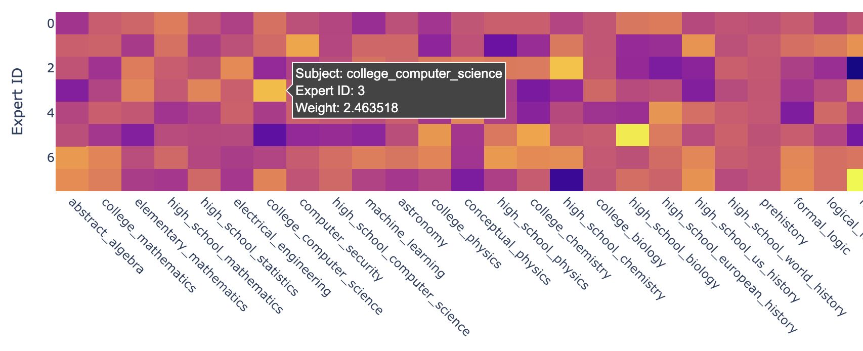
- Mistral has also released Mixtral 8x7B Instruct v0.1 trained using supervised fine-tuning and direct preference optimization (DPO). It scores 8.3 on MT-Bench making it the best open-source model, with performance comparable to GPT3.5.
- Mistral offers three chat endpoints with competitive pricing via Mistral AI La Plateforme:
- Mistral-tiny: Mistral 7B Instruct v0.2, upgraded base model with higher context length 8K \(\rightarrow\) 32K and better finetuning, 6.84 \(\rightarrow\) 7.61 on MT Bench.
- Mistral-small: Mistral 8x7B Instruct v0.1, matches or exceeds GPT-3.5 performance, multilingual.
- Mistral-medium: Outperforms GPT-3.5 on all metrics, multilingual.
- They’ve also announced Mistral-embed, an embedding model with a 1024 embedding dimension, which achieves 55.26 on MTEB.
- Refer MoE Explanation.
- Blog; La Plateforme; Mixtral-8x7B-v0.1 Base model; Mixtral-8x7B-v0.1 Instruct model.
Results
- Benchmark results comparing against the other SOTA OSS models as of this writing: LLaMA-2, Yi-34B (from 01.AI led by Kai-Fu Lee), and DeepSeek-67B (a strong model made by a quant trading company).
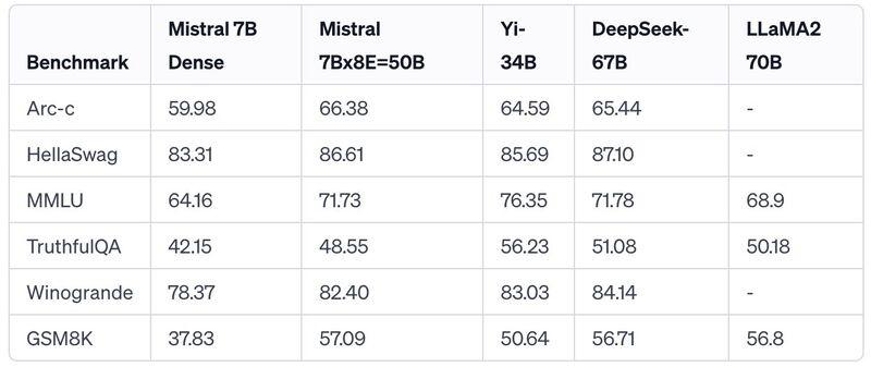
OpenMoE
- OpenMoE, one of the earliest open-source MoE implementations, is a family of open-sourced MoE LLMs.
- Related: Colossal AI’s PyTorch OpenMoE implementation including both training and inference with expert parallelism.
Learning Resources
A Visual Guide to Mixture of Experts (MoE)
- A deep-dive into the MoE architecture. Goes into details about what the separate experts learn, how to route between them, vision-MoE.
Related Papers
Outrageously Large Neural Networks: The Sparsely-Gated Mixture-of-Experts Layer
- The capacity of a neural network to absorb information is limited by its number of parameters. Conditional computation, where parts of the network are active on a per-example basis, has been proposed in theory as a way of dramatically increasing model capacity without a proportional increase in computation. In practice, however, there are significant algorithmic and performance challenges. Also, static neural network architectures apply the same function to every example. In contrast, input dependent models attempt to tailor the function to each example. While it is straightforward for a human to manually specify a single static architecture, it is infeasible to specify every input-dependent function by hand. Instead, the input-dependent function must be automatically inferred by the model, which introduces an extra level of complexity in optimization.
- Given the need to automatically infer architectures for each example, a natural solution is to define a single large model (supernetwork) with a numerous sub-networks (experts), and route examples through a path in the supernetwork. The figure below from Ramachandran and Le (2019) visualizes an example of a routing network.. Intuitively, similar examples can be routed through similar paths and dissimilar examples can be routed through different paths. The example-dependent routing also encourages expert specialization, in which experts devote their representational capacity to transforming a chosen subset of examples.
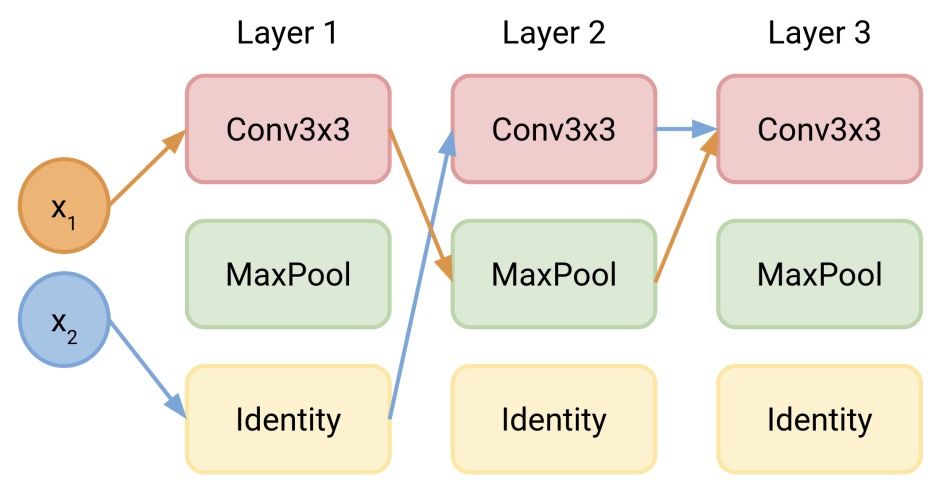
- Learning to route examples to well-matched experts is critical for good performance. Effective routing can be achieved by training another small neural network (router) that learns to route examples through the supernetwork. The router takes the example as input and outputs the next expert to use. The router can take advantage of the intermediate representations of the example produced in the supernetwork.
- This paper by Shazeer et al. in ICLR 2017 addresses these challenges and finally realize the promise of conditional computation, achieving greater than 1000x improvements in model capacity with only minor losses in computational efficiency on modern GPU clusters.
- They introduce a Sparsely-Gated Mixture-of-Experts layer (MoE), consisting of up to thousands of feed-forward sub-networks. A trainable gating network determines a sparse combination of these experts to use for each example. In this per-example routing setup, different examples are processed by different subcomponents, or experts, inside a larger model, a.k.a. a supernetwork.
- Specifically, the proposed MoE layer takes as an input a token representation \(x\) and then routes this to the best determined top-\(k\) experts, selected from a set \(\left\{E_i(x)\right\}_{i=1}^N\) of \(N\) experts. The router variable \(W_r\) produces logits \(h(x)=W_r \cdot x\) which are normalized via a softmax distribution over the available \(N\) experts at that layer. The gate-value for expert \(i\) is given by,
- The top-\(k\) gate values are selected for routing the token \(x\). If \(\mathcal{T}\) is the set of selected top-\(k\) indices then the output computation of the layer is the linearly weighted combination of each expert’s computation on the token by the gate value,
- They apply the MoE to the tasks of language modeling and machine translation, where model capacity is critical for absorbing the vast quantities of knowledge available in the training corpora. We present model architectures in which a MoE with up to 137 billion parameters is applied convolutionally between stacked LSTM layers. On large language modeling and machine translation benchmarks, these models achieve significantly better results than state-of-the-art at lower computational cost.
- The following diagram from the paper illustrates a Mixture of Experts (MoE) layer embedded within a recurrent language model. In this case, the sparse gating function selects two experts to perform computations. Their outputs are modulated by the outputs of the gating network.
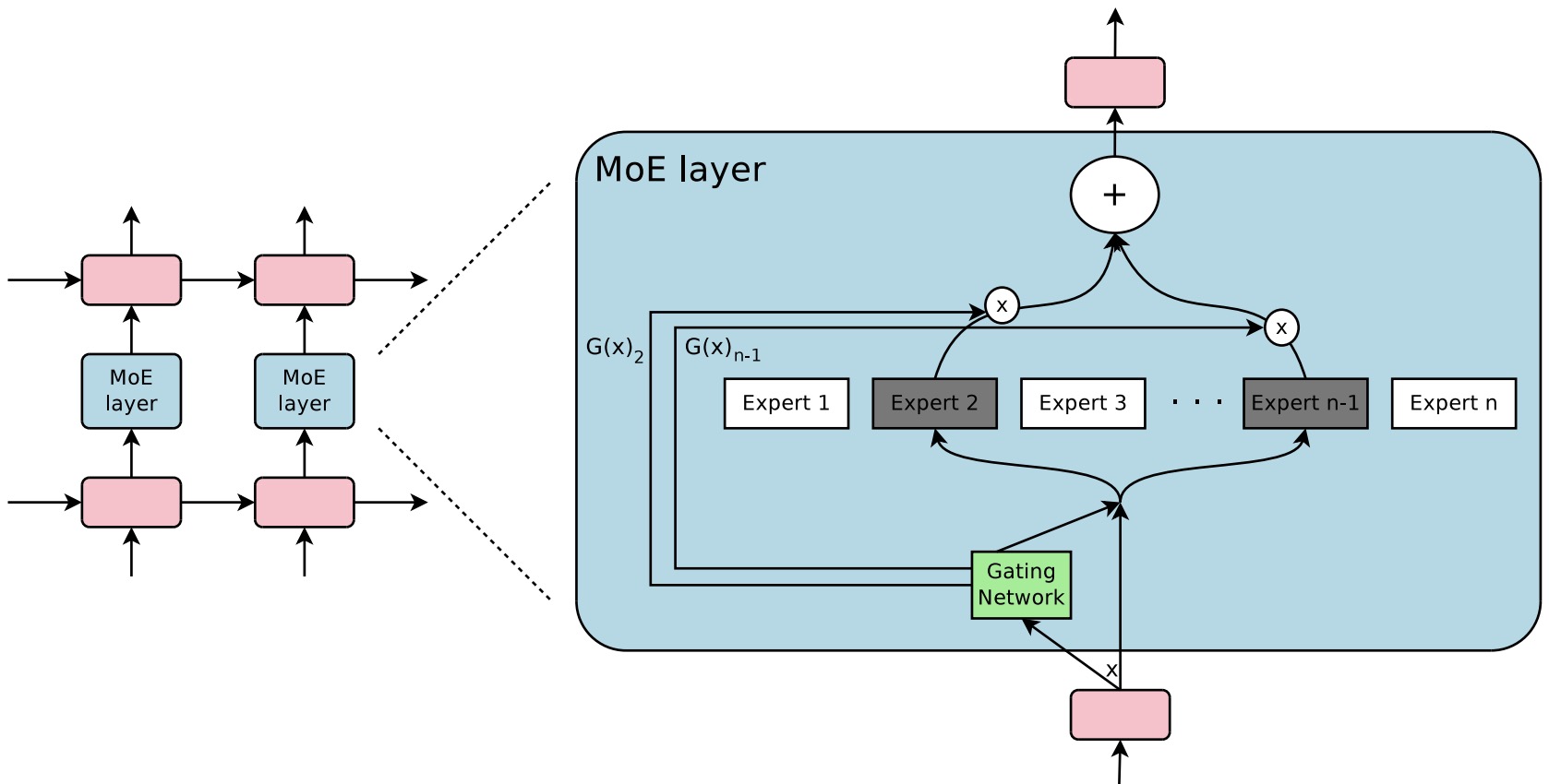
Scaling Vision with Sparse Mixture of Experts
- Almost all prevalent computer vision models networks are “dense,” that is, every input is processed by every parameter.
- This paper by Riquelme et al. from Google Brain introduces the Vision Mixture of Experts (V-MoE), a novel approach for scaling vision models. The V-MoE is a sparsely activated version of the Vision Transformer (ViT) that demonstrates scalability and competitiveness with larger dense networks in image recognition tasks.
- The paper proposes a sparse variant of the Vision Transformer (ViT) that uses a mixture-of-experts architecture. This approach routes each image patch to a subset of experts, making it possible to scale up to 15B parameters while matching the performance of state-of-the-art dense models.
- An innovative extension to the routing algorithm is presented, allowing prioritization of subsets of each input across the entire batch. This adaptive per-image compute leads to a trade-off between performance and computational efficiency during inference.
- The figure below from the paper shows an overview of the architecture. V-MoE is composed of \(L\) ViT blocks. In some, we replace the MLP with a sparsely activated mixture of MLPs. Each MLP (the expert) is stored on a separate device, and processes a fixed number of tokens. The communication of these tokens between devices is shown in this example, which depicts the case when \(k=1\) expert is selected per token. Here each expert uses a capacity ratio \(C=\frac{4}{3}\): the sparse MoE layer receives 12 tokens per device, but each expert has capacity for \(16\left(\frac{16 \cdot 1}{12}=\frac{4}{3}\right.\)). Non-expert components of V-MoE such as routers, attention layers and normal MLP blocks are replicated identically across devices.
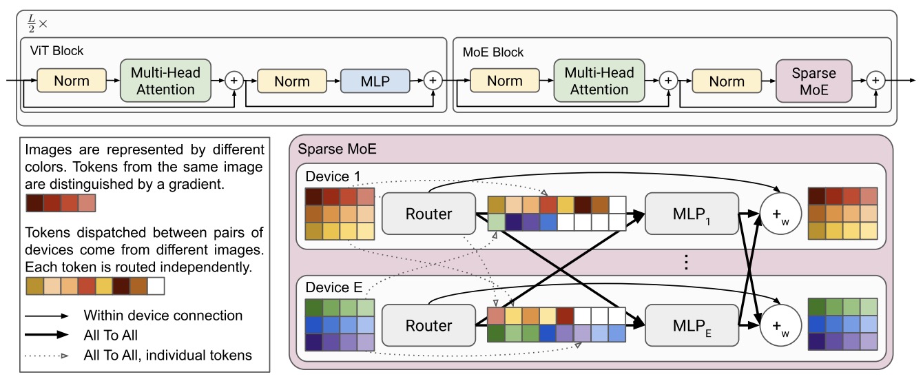
- The V-MoE shows impressive scalability, successfully trained up to 15B parameters, and demonstrates strong performance, including 90.35% accuracy on ImageNet.
- The paper explores the transfer learning abilities of V-MoE, showing its adaptability and effectiveness across different tasks and datasets, even with limited data.
- A detailed analysis of the V-MoE’s routing decisions and the behavior of its experts is provided, offering insights into the model’s internal workings and guiding future improvements.
- V-MoE models require less computational resources than dense counterparts, both in training and inference, thanks to their sparsely activated nature and the efficient use of the Batch Prioritized Routing algorithm.
- The paper concludes with the potential of sparse conditional computation in vision tasks, emphasizing the environmental benefits due to reduced CO2 emissions and the promising directions for future research in large-scale multimodal or video modeling.
- The paper represents a significant advancement in the field of computer vision, particularly in the development of scalable and efficient vision models.
Modeling Task Relationships in Multi-task Learning with Multi-gate Mixture-of-Experts
- This paper by Ma et al. published in KDD 2018, introduces a novel approach to multi-task learning called Multi-gate Mixture-of-Experts (MMoE). The method aims to enhance the performance of multi-task learning models by better handling the relationships between different tasks.
- The MMoE model adapts the MoE framework to multi-task learning by sharing expert submodels across all tasks and using a gating network optimized for each task. This design allows the model to dynamically allocate shared and task-specific resources, efficiently handling tasks with varying degrees of relatedness.
- The paper presents experiments using synthetic data and real datasets, including a binary classification benchmark and a large-scale content recommendation system at Google. These experiments demonstrate MMoE’s effectiveness in scenarios where tasks have low relatedness and its superiority over traditional shared-bottom multi-task models in terms of both performance and trainability.
- MMoE’s architecture consists of multiple experts (feed-forward networks) and a gating network for each task, which determines the contribution of each expert to the task. This setup allows the model to learn nuanced relationships between tasks and allocate computation resources more effectively.
- The following figure from the paper shows a (a) shared-Bottom model, (b) one-gate MoE model, (c) multi-gate MoE model.
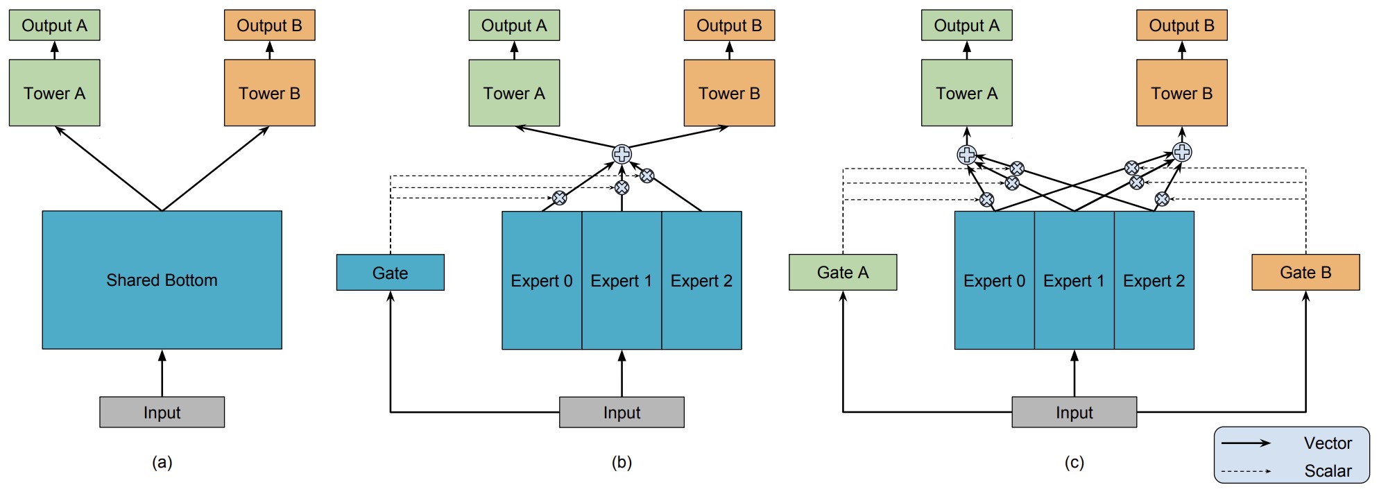
- In the experiments with the Census-income dataset, a UCI benchmark dataset, the task was to predict whether an individual’s income exceeds $50,000 based on census data. The dataset contains demographic and employment-related information. MMoE’s application to this dataset involved addressing the challenge of binary classification using multiple socio-economic factors as input features.
- On synthetic data, MMoE showed better performance, especially when task correlation is low, and demonstrated improved trainability with less variance in model performance across runs. On real-world datasets, including the UCI Census-income dataset and Google’s content recommendation system, MMoE consistently outperformed baseline models in terms of accuracy and robustness.
- MMoE offers computational efficiency by using lightweight gating networks and shared expert networks, making it suitable for large-scale applications. The experiments on Google’s recommendation system highlighted MMoE’s ability to improve both engagement and satisfaction metrics in live experiments compared to single-task and shared-bottom models.
Mixture-of-Experts Meets Instruction Tuning: A Winning Combination for Large Language Models
- The paper titled “Mixture-of-Experts Meets Instruction Tuning: A Winning Combination for Large Language Models” presents an innovative approach to enhancing the performance and scalability of Large Language Models (LLMs) by combining Sparse MoE architecture with instruction tuning. - Sparse MoE is a neural architecture that adds learnable parameters to LLMs without increasing inference costs. In contrast, instruction tuning trains LLMs to follow instructions more effectively.
- The authors advocate for the combination of these two approaches, demonstrating that MoE models benefit significantly more from instruction tuning compared to their dense model counterparts.
- The paper presents three experimental setups: direct finetuning on individual downstream tasks without instruction tuning; instruction tuning followed by few-shot or zero-shot generalization on downstream tasks; and instruction tuning supplemented by further finetuning on individual tasks.
- The findings indicate that MoE models generally underperform compared to dense models of the same computational capacity in the absence of instruction tuning. However, this changes with the introduction of instruction tuning, where MoE models outperform dense models.
- The paper introduces the FLAN-MOE32B model, which outperforms FLAN-PALM62B on four benchmark tasks while using only a third of the FLOPs. This highlights the efficiency and effectiveness of the FLAN-MOE approach.
- The authors conduct a comprehensive series of experiments to compare the performance of various MoE models subjected to instruction tuning. These experiments include evaluations in natural language understanding, reasoning, and question-answering tasks. The study also explores the impact of different routing strategies and the number of experts on the performance of FLAN-MOE models, showing that performance scales with the number of tasks rather than the number of experts.
- The following image from the paper shows the effect of instruction tuning on MOE models versus dense counterparts for base-size models (same flops across all models in this figure). They perform single-task finetuning for each model on held-out benchmarks. Compared to dense models, MoE models benefit more from instruction-tuning, and are more sensitive to the number of instruction-tuning tasks. Overall, the performance of MoE models scales better with respect to the number of tasks, than the number of experts.
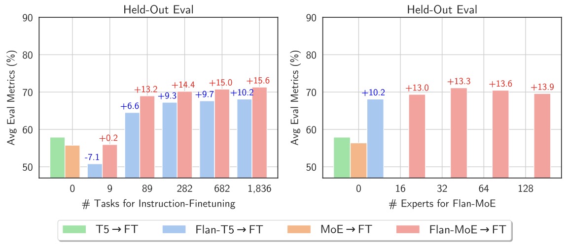
- The paper discusses the challenge of adapting MoE models to multilingual benchmarks and highlights the importance of incorporating diverse linguistic data during training to ensure effective language coverage.
- Overall, the paper “Mixture-of-Experts Meets Instruction Tuning” by Sheng Shen et al. presents significant advancements in the scalability and efficiency of LLMs through the novel integration of MoE architecture and instruction tuning, setting new standards in the field of natural language processing.
From Sparse to Soft Mixtures of Experts
- Sparse Mixture of Experts (MoE) architectures scale model capacity without large increases in training or inference costs. MoE allows us to dramatically scale model sizes without significantly increasing inference latency. In short, each “expert” can separately attend to a different subset of tasks via different data subsets before they are combined via an input routing mechanism. Thus, the model can learn a wide variety of tasks, but still specialize when appropriate. Despite their success, MoEs suffer from a number of issues: training instability, token dropping, inability to scale the number of experts, or ineffective finetuning.
- This paper by Puigcerver et al. from Google DeepMind proposes Soft MoE, a fully-differentiable sparse Transformer that addresses these challenges, while maintaining the benefits of MoEs.
- Extra-large models like Google’s PaLM (540B parameters) or OpenAI’s GPT-4 use Sparse MoE under the hood, which suffers from training instabilities, because it’s not fully differentiable. Soft-MoE replaces the non-differentiable expert routing with a differentiable layer. The end-to-end model is fully differentiable again, can be trained with ordinary SGD-like optimizers, and the training instabilities go away.
- Soft MoE performs an implicit soft assignment by passing different weighted combinations of all input tokens to each expert. As in other MoE works, experts in Soft MoE only process a subset of the (combined) tokens, enabling larger model capacity at lower inference cost.
- The following figure from the paper illustrates the main differences between Sparse and Soft MoE layers. While the router in Sparse MoE layers (left) learns to assign individual input tokens to each of the available slots, in Soft MoE layers (right) each slot is the result of a (different) weighted average of all the input tokens. Learning to make discrete assignments introduces several optimization and implementation issues that Soft MoE sidesteps.
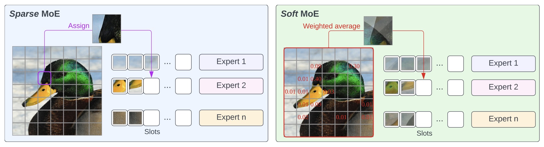
- They propose a fully-differentiable sparse vision transformer (ViT) that addresses aforementioned challenges such as training instability, token dropping, and inefficient finetuning. In the context of visual recognition, Soft MoE greatly outperforms the standard ViT and popular MoE variants (Tokens Choice and Experts Choice). Soft MoE scales ViT models to >50B parameters with little effect on inference latency. For example, Soft MoE-Base/16 requires 10.5x lower inference cost (5.7x lower wall-clock time) than ViT-Huge/14 while matching its performance after similar training. Soft MoE also scales well: Soft MoE Huge/14 with 128 experts in 16 MoE layers has over 40x more parameters than ViT Huge/14, while inference time cost grows by only 2%, and it performs substantially better.
- The following figure from the paper illustrates the Soft MoE routing algorithm. Soft MoE first computes scores or logits for every pair of input token and slot, based on some learnable per-slot parameters. These logits are then normalized per slot (columns) and every slot computes a linear combination of all the input tokens based on these weights (in green). Each expert (an MLP in this work) then processes its slots (e.g. 2 slots per expert, in this diagram). Finally, the same original logits are normalized per token (i.e., by row) and used to combine all the slot outputs, for every input token (in blue). Dashed boxes represent learnable parameters.
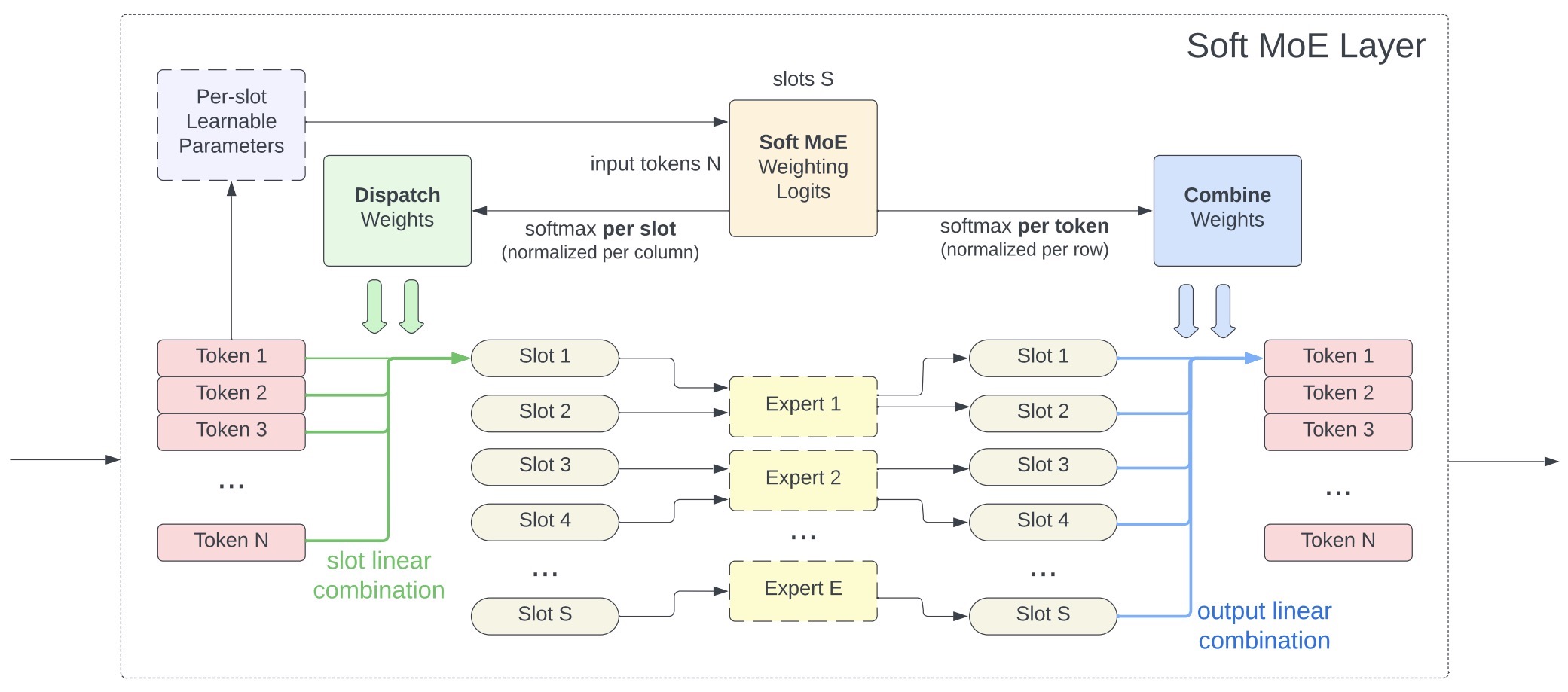
- The following infographic (source) presents an overview of their results:
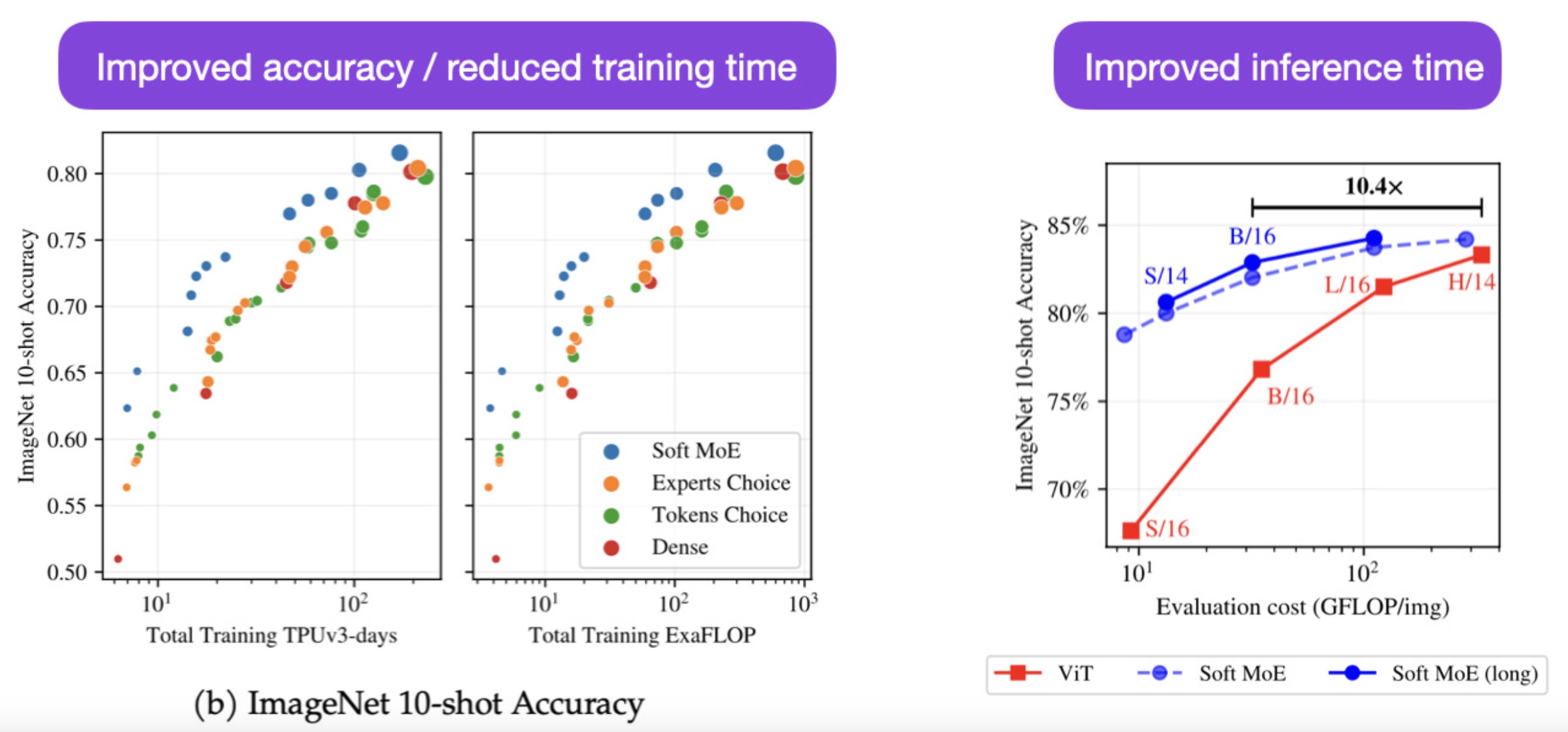
- PyTorch implementation.
Switch Transformers
- Proposed in Switch Transformers: Scaling to Trillion Parameter Models with Simple and Efficient Sparsity.
- In deep learning, models typically reuse the same parameters for all inputs. Mixture of Experts (MoE) defies this and instead selects different parameters for each incoming example. The result is a sparsely-activated model – with outrageous numbers of parameters – but a constant computational cost.
- This paper by Fedus et al. from Google in JMLR 2022 introduces the Switch Transformer which seeks to address the lack of widespread adoption of MoE which has been hindered by complexity, communication costs, and training instability.
- They simplify the MoE routing algorithm and design intuitive improved models with reduced communication and computational costs. Our proposed training techniques help wrangle the instabilities and they show large sparse models may be trained, for the first time, with lower precision (bfloat16) formats.
- The guiding design principle for Switch Transformers is to maximize the parameter count of a Transformer model (Vaswani et al., 2017) in a simple and computationally efficient way. The benefit of scale was exhaustively studied in Kaplan et al. (2020) which uncovered powerlaw scaling with model size, data set size and computational budget. Importantly, this work advocates training large models on relatively small amounts of data as the computationally optimal approach. Heeding these results, they investigate a fourth axis: increase the parameter count while keeping the floating point operations (FLOPs) per example constant. Our hypothesis is that the parameter count, independent of total computation performed, is a separately important axis on which to scale. They achieve this by designing a sparsely activated model that efficiently uses hardware designed for dense matrix multiplications such as GPUs and TPUs. In their distributed training setup, their sparsely activated layers split unique weights on different devices. Therefore, the weights of the model increase with the number of devices, all while maintaining a manageable memory and computational footprint on each device.
- Their switch routing proposal reimagines MoE. Shazeer et al. (2017) conjectured that routing to \(k > 1\) experts was necessary in order to have non-trivial gradients to the routing functions. The authors intuited that learning to route would not work without the ability to compare at least two experts. Ramachandran and Le (2018) went further to study the top-\(k\) decision and found that higher \(k\)-values in lower layers in the model were important for models with many routing layers. Contrary to these ideas, they instead use a simplified strategy where they route to only a single expert. They show this simplification preserves model quality, reduces routing computation and performs better. This \(k = 1\) routing strategy is later referred to as a Switch layer.
- The following figure from the paper illustrates the Switch Transformer encoder block. We replace the dense feed forward network (FFN) layer present in the Transformer with a sparse Switch FFN layer (light blue). The layer operates independently on the tokens in the sequence. They diagram two tokens (\(x_1\) = “More” and \(x_2\) = “Parameters” below) being routed (solid lines) across four FFN experts, where the router independently routes each token. The switch FFN layer returns the output of the selected FFN multiplied by the router gate value (dotted-line).
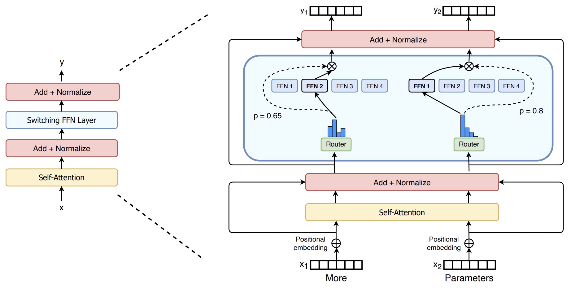
- They design models based off T5-Base and T5-Large to obtain up to 7x increases in pre-training speed with the same computational resources. These improvements extend into multilingual settings where they measure gains over the mT5-Base version across all 101 languages.
- Finally, they advance the current scale of language models by pre-training up to trillion parameter models on the “Colossal Clean Crawled Corpus” and achieve a 4x speedup over the T5-XXL model.
- Code.
QMoE: Practical Sub-1-Bit Compression of Trillion-Parameter Models
- This paper by Frantar and Alistarh from the Institute of Science and Technology Austria and Neural Magic Inc. presents QMoE, a framework designed to address the memory challenges in deploying large language models (LLMs) with MoE architectures.
- The key problem QMoE addresses is the massive memory requirement of large models, exemplified by the 1.6 trillion-parameter SwitchTransformer-c2048 model, which typically requires 3.2TB of memory. QMoE effectively compresses such models to less than 1 bit per parameter, enabling their execution on commodity hardware with minor runtime overheads.
- QMoE employs a scalable algorithm and a custom compression format paired with GPU decoding kernels. It compresses the SwitchTransformer-c2048 model to less than 160GB (0.8 bits per parameter) with minor accuracy loss in under a day on a single GPU.
- The implementation includes a highly scalable compression algorithm and a bespoke compression format, facilitating efficient end-to-end compressed inference. The framework enables running trillion-parameter models on affordable hardware, like servers equipped with NVIDIA GPUs, at less than 5% runtime overhead compared to ideal uncompressed execution.
- The paper discusses the challenges in compressing MoE models, including conceptual issues with existing post-training compression methods and practical scaling challenges. It overcomes these by introducing a custom compression format and highly-efficient decoding algorithms optimized for GPU accelerators.
- The technical contributions include a novel approach to handling massive activation sets and a unique system design for optimized activation offloading, expert grouping, and robustness modifications, ensuring efficient application of data-dependent compression to massive MoEs.
- The framework significantly reduces the size of large models, with QMoE compressed models achieving over 20x compression rates compared to 16-bit precision models. This reduction in size is accompanied by minor increases in loss on pretraining validation and zero-shot data.
- The paper also discusses the system design and optimizations made to address memory costs, GPU utilization, and reliability requirements. These include techniques like optimized activation offloading, list buffer data structures, lazy weight fetching, and expert grouping.
- The following figure from the paper illustrates the offloading execution for the sparse part of a Transformer block. An expert \(E_2\) and its corresponding input tokens \(X_E\) are fetched to GPU memory to produce \(E_2′\), which together with the corresponding outputs \(Y_E\) are written back to CPU again.
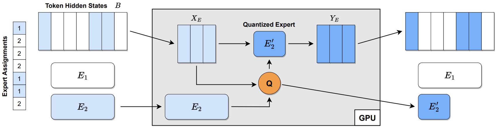
- The experiments demonstrate that QMoE effectively compresses MoE models while maintaining performance. The system was tested on various datasets, including Arxiv, GitHub, StackExchange, and Wikipedia, showing good performance preservation even for highly compressed models.
- The paper provides detailed insights into the encoding and decoding processes and the kernel implementation for the GPU, highlighting the challenges and solutions for achieving sub-1-bit per parameter compression.
- The QMoE framework is a significant step towards practical deployment of massive-scale MoE models, addressing key limitations of MoE architectures and facilitating further research and understanding of such models.
- The paper’s findings are significant as they make it feasible to deploy and research trillion-parameter models on more accessible hardware, potentially democratizing access to high-performance LLMs and spurring further innovation in the field.
MegaBlocks: Efficient Sparse Training with Mixture-of-Experts
- This paper by Gale et al. from Stanford University, Microsoft Research, and Google Research, introduces Dropless MoE, a novel system for efficient MoE training on GPUs.
- The system, named MegaBlocks, addresses the limitations of current frameworks that restrict dynamic routing in MoE layers, often leading to a tradeoff between model quality and hardware efficiency due to the necessity of dropping tokens or wasting computation on excessive padding. Token dropping leads to information loss, as it involves selectively ignoring part of the input data, while padding adds redundant data to make the varying input sizes uniform, which increases computational load without contributing to model learning. This challenge arises from the difficulty in efficiently handling the dynamic routing and load-imbalanced computation characteristic of MoE architectures, especially in the context of deep learning hardware and software constraints.
- MegaBlocks innovatively reformulates MoE computations as block-sparse operations, developing new GPU kernels specifically for this purpose. These kernels efficiently manage dynamic, load-imbalanced computations inherent in MoEs without resorting to token dropping. This results in up to 40% faster end-to-end training compared to MoEs trained with the Tutel library, and 2.4 times speedup over DNNs trained with Megatron-LM.
- The system’s core contributions include high-performance GPU kernels for block-sparse matrix multiplication, leveraging blocked-CSR-COO encoding and transpose indices. This setup enables efficient handling of sparse inputs and outputs in both transposed and non-transposed forms.
- Built upon the Megatron-LM library for Transformer model training, MegaBlocks supports distributed MoE training with data and expert model parallelism. Its unique ability to avoid token dropping through block-sparse computation provides a fresh approach to MoE algorithms as a form of dynamic structured activation sparsity.
- The figure below from the paper shows a Mixture-of-Experts Layer. Shown for
num experts=3,top k=1andcapacity factor=1with the prevalent, token dropping formulation. First (1), tokens are mapped to experts by the router. Along with expert assignments, the router produces probabilities that reflect the confidence of the assignments. Second (2), the feature vectors are permuted to group tokens by expert assignment. If the number of tokens assigned to an expert exceeds its capacity, extra tokens are dropped. Third (3), the expert layers are computed for the set of tokens they were assigned as well as any padding needed for unused capacity. Lastly (4), the results of the expert computation are un-permuted and weighted by the router probabilities. The outputs for dropped tokens are shown here set to zero.
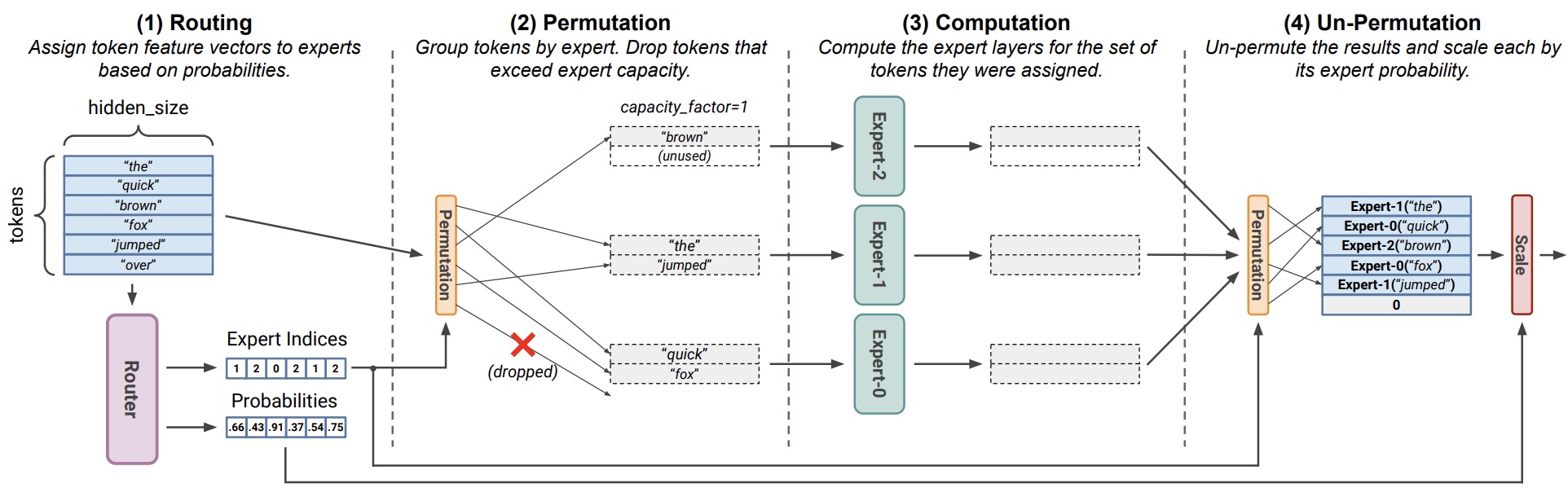
- Experiments demonstrate that MegaBlocks enables significant end-to-end training speedups for MoE models compared to existing approaches, especially as model size increases. The system also reduces the computational overhead and memory requirements associated with MoE layers, leading to more efficient utilization of hardware resources. Furthermore, the approach decreases the number of hyperparameters that need to be re-tuned for each model and task, simplifying the process of training large MoE models.
- The paper provides detailed insights into the design and performance of the block-sparse kernels, including analyses of throughput relative to cuBLAS batched matrix multiplication and discussions on efficient routing and permutation for MoEs. The results show that MegaBlocks’ kernels perform comparably to cuBLAS, achieving an average of 98.6% of cuBLAS’s throughput with minimal variations across different configurations.
- Code
MoE-LLaVA: Mixture of Experts for Large Vision-Language Models
- This paper by Lin et al. from Peking University, Sun Yat-sen University, FarReel Ai Lab, Tencent Data Platform, and Peng Cheng Laboratory introduces MoE-LLaVA, a novel training strategy for Large Vision-Language Models (LVLMs). The strategy, known as MoE-tuning, constructs a sparse model with a large number of parameters while maintaining constant computational costs and effectively addressing performance degradation in multi-modal learning and model sparsity.
- MoE-LLaVA uniquely activates only the top-\(k\) experts through routers during deployment, keeping the remaining experts inactive. This approach results in impressive visual understanding capabilities and reduces hallucinations in model outputs. Remarkably, with 3 billion sparsely activated parameters, MoE-LLaVA performs comparably to the LLaVA-1.5-7B and surpasses the LLaVA-1.5-13B in object hallucination benchmarks.
- The architecture of MoE-LLaVA includes a vision encoder, a visual projection layer (MLP), a word embedding layer, multiple stacked LLM blocks, and MoE blocks. The MoE-tuning process involves three stages: In Stage I, an MLP adapts visual tokens to the LLM. Stage II trains the whole LLM’s parameters except for the Vision Encoder (VE), and in Stage III, FFNs are used to initialize the experts in MoE, and only the MoE layers are trained.
- The following image from the paper illustrates MoE-tuning. The MoE-tuning consists of three stages. In stage I, only the MLP is trained. In stage II, all parameters are trained except for the Vision Encoder (VE). In stage III, FFNs are used to initialize the experts in MoE, and only the MoE layers are trained. For each MoE layer, only two experts are activated for each token, while the other experts remain silent.
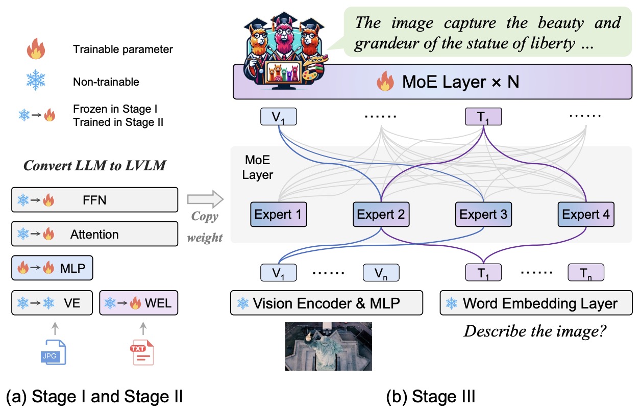
- The model was evaluated on various visual understanding datasets, demonstrating its efficiency and effectiveness. MoE-LLaVA’s performance was on par with or even superior to state-of-the-art models with fewer activated parameters. The paper also includes extensive ablation studies and visualizations to illustrate the effectiveness of the MoE-tuning strategy and the MoE-LLaVA architecture.
- The paper provides a significant contribution to the field of multi-modal learning systems, offering insights for future research in developing more efficient and effective systems.
- Code
Mixture of LoRA Experts
- This paper by Wu et al. from MSR Asia and Tsinghua University, published in ICLR 2024, proposes Mixture of LoRA Experts (MOLE), focusing on efficient composition of Low-Rank Adaptation (LoRA) techniques. It addresses the challenge of effectively integrating multiple trained LoRAs, a method previously developed to fine-tune large pre-trained models with minimal computational overhead.
- MOLE employs a hierarchical weight control approach where each layer of a LoRA is treated as an expert. By integrating a learnable gating function within each layer, MOLE determines optimal composition weights tailored to specific domain objectives. This method enhances the performance of LoRA compositions and preserves their flexibility, addressing the limitations of linear arithmetic and reference tuning-based compositions which either diminish generative capabilities or involve high training costs.
- The figure below from the paper illustrates an overview of LoRA composition methods: (a) Linear arithmetic composition, which commonly applies the same composition weight \(\boldsymbol{W}_i\) to all layers of the \(i^{\text {th}}\) LoRA. (b) Reference tuning-based composition involves retraining a large model by integrating outputs from multiple LoRAs using manually-crafted mask information. (c) Our MoLE, which learns a distribution \(\Upsilon^j\) for the \(j^{\text {th}}\) layer of LoRAs to determine the composition weight \(\boldsymbol{W}_i^j\).

- During the training phase, MOLE predicts weights for each expert using a gating function while keeping other parameters frozen, resulting in minimal computational costs. In the inference phase, MOLE can utilize all trained LoRAs with preserved characteristics or allow for manual masking of LoRAs to adjust weights dynamically without retraining.
- The architecture incorporates gating functions at various hierarchical levels to effectively manage the contributions of different LoRA layers. The paper details two distinct inference modes facilitated by MOLE, enhancing its adaptability across various scenarios and tasks in both NLP and Vision & Language domains.
- The figure below from the paper illustrates the orkflow of MOLE. In the training phase, MOLE predicts weights for multiple LoRAs. In the inference phase, MOLE can allocate weights to multiple LoRAs, or, without altering the gating weights, achieve a more flexible LoRA composition by masking out undesired LoRAs and recalculating and distributing weights proportionally.

- Extensive experiments demonstrate that MOLE outperforms existing LoRA composition methods in terms of both qualitative and quantitative measures. Results from NLP and Vision & Language tasks illustrate that MOLE consistently achieves superior performance compared to traditional composition methods, validating its approach in a real-world setting.
- Code
JetMoE: Reaching Llama2 Performance with 0.1M Dollars
- This paper by Shen et al. from MIT-IBM Watson AI Lab, MIT EECS, Princeton University, and MyShell.ai & MIT introduces JetMoE-8B, a cost-effective large language model developed at the MIT-IBM Watson AI Lab, outperforming established models like Llama2-7B and Llama2-13B-Chat. JetMoE-8B extends the concept of sparse activation to both the attention and feed-forward layers. Despite being trained on a tight budget of under $100,000, JetMoE-8B employs 8 billion parameters, leveraging a Sparsely-gated Mixture-of-Experts (SMoE) architecture that activates only 2 billion parameters per input token. This architecture reduces inference computation by approximately 70% compared to Llama2-7B.
- JetMoE-8B is trained using the Megatron framework with Megablock enhancements, using pipeline parallelism to optimize computational costs and load balance during training. Notably, it incorporates innovations like shared KV projection in attention layers and a frequency-based auxiliary loss for training efficiency.
- The figure below from the paper illustrates the JetMoE architecture.

- For pretraining, JetMoE-8B utilized a mixture of real-world and synthetic datasets, totaling 1.25 trillion tokens. Datasets include RefinedWeb, StarCoder, and various components from The Pile, combined with synthetic datasets like OpenHermes 2.5 for diverse training inputs.
- Utilized a two-phase training approach, incorporating a mix of real and synthetic datasets with adjustments in data weighting during the learning rate decay phase to enhance model performance.
- The model underwent Distilled Supervised Fine-Tuning (dSFT) and Distilled Direct Preference Optimization (dDPO), refining model responses based on preferences from a teacher model to improve alignment with human-like conversational abilities.
- JetMoE-8B’s performance was benchmarked against other models in tasks like ARC-challenge, Hellaswag, and MMLU, showing superior performance in many areas, particularly in code-related benchmarks like MBPP and HumanEval.
- The training parameters, model configurations, and data mixtures are fully documented and made open-source to foster further academic and practical advancements in efficient LLM training methodologies.
- Code
QMoE: Practical Sub-1-Bit Compression of Trillion-Parameter Models
- This paper by Frantar and Alistarh from the Institute of Science and Technology Austria and Neural Magic Inc. presents QMoE, a framework designed to address the memory challenges in deploying large language models (LLMs) with MoE architectures.
- The key problem QMoE addresses is the massive memory requirement of large models, exemplified by the 1.6 trillion-parameter SwitchTransformer-c2048 model, which typically requires 3.2TB of memory. QMoE effectively compresses such models to less than 1 bit per parameter, enabling their execution on commodity hardware with minor runtime overheads.
- QMoE employs a scalable algorithm and a custom compression format paired with GPU decoding kernels. It compresses the SwitchTransformer-c2048 model to less than 160GB (0.8 bits per parameter) with minor accuracy loss in under a day on a single GPU.
- The implementation includes a highly scalable compression algorithm and a bespoke compression format, facilitating efficient end-to-end compressed inference. The framework enables running trillion-parameter models on affordable hardware, like servers equipped with NVIDIA GPUs, at less than 5% runtime overhead compared to ideal uncompressed execution.
- The paper discusses the challenges in compressing MoE models, including conceptual issues with existing post-training compression methods and practical scaling challenges. It overcomes these by introducing a custom compression format and highly-efficient decoding algorithms optimized for GPU accelerators.
- The technical contributions include a novel approach to handling massive activation sets and a unique system design for optimized activation offloading, expert grouping, and robustness modifications, ensuring efficient application of data-dependent compression to massive MoEs.
- The framework significantly reduces the size of large models, with QMoE compressed models achieving over 20x compression rates compared to 16-bit precision models. This reduction in size is accompanied by minor increases in loss on pretraining validation and zero-shot data.
- The paper also discusses the system design and optimizations made to address memory costs, GPU utilization, and reliability requirements. These include techniques like optimized activation offloading, list buffer data structures, lazy weight fetching, and expert grouping.
- The following figure from the paper illustrates the offloading execution for the sparse part of a Transformer block. An expert \(E_2\) and its corresponding input tokens \(X_E\) are fetched to GPU memory to produce \(E_2′\), which together with the corresponding outputs \(Y_E\) are written back to CPU again.
- The experiments demonstrate that QMoE effectively compresses MoE models while maintaining performance. The system was tested on various datasets, including Arxiv, GitHub, StackExchange, and Wikipedia, showing good performance preservation even for highly compressed models.
- The paper provides detailed insights into the encoding and decoding processes and the kernel implementation for the GPU, highlighting the challenges and solutions for achieving sub-1-bit per parameter compression.
- The QMoE framework is a significant step towards practical deployment of massive-scale MoE models, addressing key limitations of MoE architectures and facilitating further research and understanding of such models.
- The paper’s findings are significant as they make it feasible to deploy and research trillion-parameter models on more accessible hardware, potentially democratizing access to high-performance LLMs and spurring further innovation in the field.
CuMo: Scaling Multimodal LLM with Co-Upcycled Mixture-of-Experts
-
This paper by Li et al. from SHI Labs (Georgia Tech & UIUC) and ByteDance introduces CuMo, a multimodal large language model (LLM) framework that scales visual understanding capabilities using Co-Upcycled MoE blocks integrated into the vision encoder and MLP connector, while maintaining minimal additional inference cost. CuMo aims to improve the scalability and efficiency of multimodal LLMs by incorporating sparsity through MoE design, especially on the vision side, which has been underexplored in previous works.
-
Core Concept and Motivation: Prior efforts in scaling multimodal LLMs focused primarily on increasing paired image-text data or enhancing LLMs, which is computationally intensive. CuMo instead targets the vision modules by integrating sparsely-gated Top-K MoE blocks to enhance capability without substantially increasing inference costs.
-
Architecture and Implementation:
-
MoE Integration:
-
CuMo inserts Top-K sparsely-gated MoE blocks into:
- Vision Encoder (CLIP-ViT): Each dense MLP block is replaced with a Top-K MoE block.
- Vision-Language MLP Connector: A two-layer MLP is replaced by a sparse MoE block.
- Each MoE block consists of multiple experts (e.g., 4 or 8), with a router network trained to select Top-K experts (usually K=2) for each input token.
- Output of MoE block: \(X_{out} = \sum_{i=1}^{K} W_i \cdot \text{MLP}_i(X)\) where \(W_i\) is the re-normalized gating weight for the \(i^{th}\) selected expert.
-
-
Training Methodology:
-
Three-Stage Training:
- Pre-training Stage: Only the MLP connector is trained using LLaVA-558K to align visual tokens with text space.
- Pre-finetuning Stage: All parameters are unfrozen and trained with high-quality captions (e.g., ALLaVA) to warm up the model.
- Visual Instruction Tuning: Final training stage with full open-sourced multimodal datasets (~1.65M samples), where the MoE blocks are incorporated and trained.
-
Co-Upcycling Initialization:
- Experts in MoE blocks are initialized from pretrained MLP layers, which stabilizes convergence and reduces training cost. This technique is referred to as co-upcycling.
- The Top-K router is trained from scratch during instruction tuning.
-
-
Loss Function:
-
Combines standard cross-entropy loss with auxiliary losses to ensure balanced expert usage: \(L = L_{ce} + \alpha_b L_b + \alpha_z L_z\) where:
- \(L_{ce}\): language modeling loss
- \(L_b\): load balancing loss
- \(L_z\): router z-loss
- Constants: \(\alpha_b = 0.1\), \(\alpha_z = 0.01\)
-
-
LLM Backbone:
- Uses Mistral-7B as base LLM.
- Authors tested upcycling LLM as well, but found pre-trained MoE models (e.g., Mixtral 8×7B) significantly better, so LLMs are not upcycled in final CuMo.
-
-
Training Datasets:
- Visual instruction tuning leverages a blend of public datasets: LLaVA-665K, ShareGPT4V, LAION-GPT-V, DocVQA, ChartQA, AI2D, InfoVQA, SynDog-EN, ALLaVA, and LIMA.
-
The following figure from the paper shows the architecture of CuMo, which incorporates sparse Top-K MoE blocks into the CLIP vision encoder and vision-language MLP connector, thereby improving the multimodal LLM capabilities from the vision side. Skip connections are omitted for simplicity.
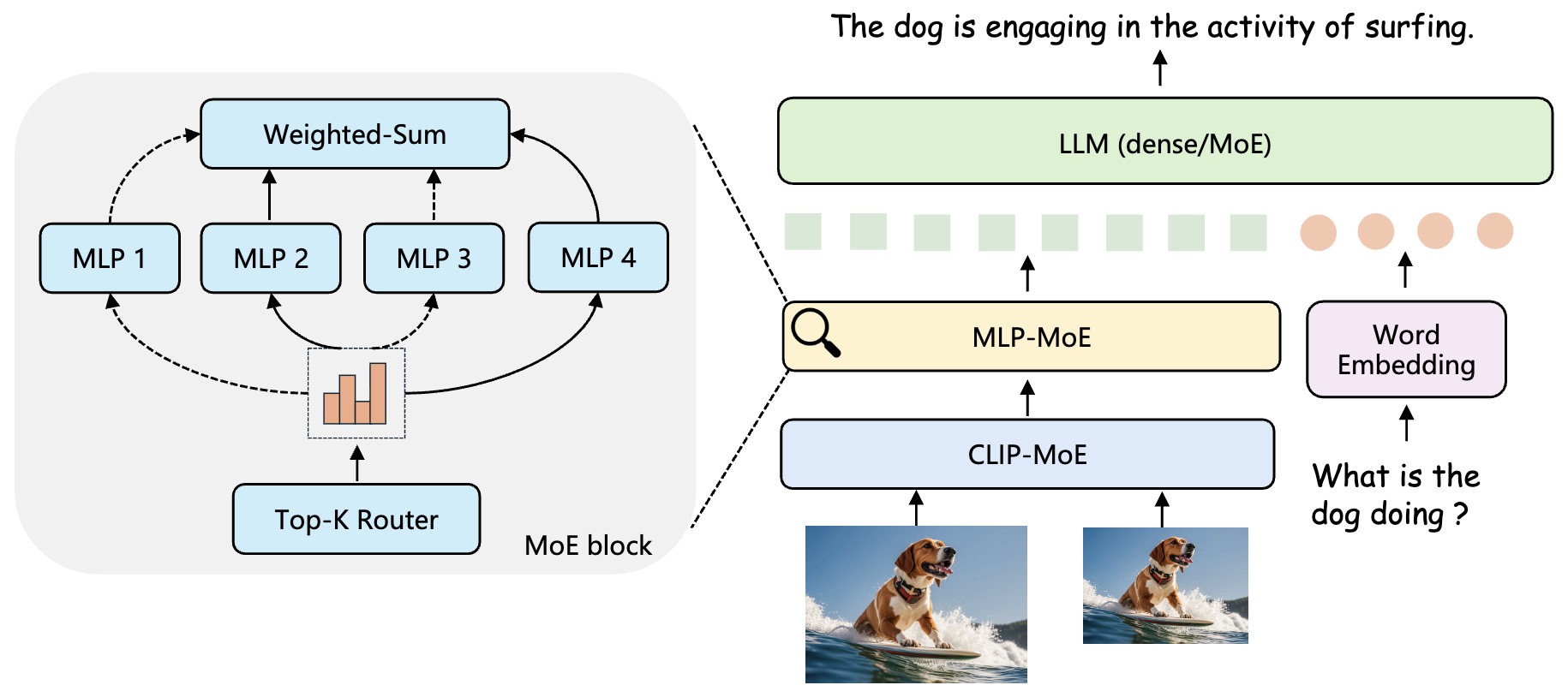
-
Benchmarks and Results:
- CuMo Mistral-7B outperforms existing 7B multimodal LLMs (e.g., LLaVA-NeXT, Mini-Gemini) and rivals many 13B models across diverse benchmarks such as VQAv2, GQA, TextVQA, MME, MMVet, and SEED-IMG.
- CuMo Mixtral-8×7B, the stronger variant, achieves top performance in the 7B MoE model group and even matches private SOTA models like MM1.
- Strong performance even under limited data settings, outperforming baselines trained with similar data volumes.
-
Ablation Studies:
- Validated that upcycling MoE blocks (vs. training from scratch) significantly stabilizes training and improves performance.
- Auxiliary bzloss (load balance + router z-loss) further improves expert utilization and model accuracy.
- Adding multi-resolution visual inputs (1× + 3×) to CLIP enhances understanding without increasing token count.
- ALLaVA-based pre-finetuning yields superior results over ShareGPT4V in the warm-up stage.
-
Qualitative Findings:
- CuMo is strong at visual grounding and reasoning, often outperforming other models in complex dialogue tasks.
- Some hallucinations remain, indicating room for improvement in response accuracy.
Branch-Train-MiX: Mixing Expert LLMs into a Mixture-of-Experts LLM
-
This paper from Sukhbaatar et al. (Meta FAIR) proposes Branch-Train-MiX (BTX), a scalable and efficient method for continued pretraining of Large Language Models (LLMs) across multiple specialized domains (e.g., math, code, knowledge) using a MoE architecture. BTX blends embarrassingly parallel expert training with sparse MoE integration, allowing a single unified model to retain and expand its capabilities across diverse domains while being finetuneable for downstream tasks.
-
Core Idea: Instead of either training a dense model on all data or training separate domain-specific experts (as in Branch-Train-Merge), BTX trains multiple domain-specific expert models in parallel and merges only their feedforward layers into MoE layers. All other modules (e.g., attention layers) are averaged across experts. The model is then finetuned to learn token-level routing, forming a unified and sparsely activated MoE LLM.
-
Architecture and Implementation:
-
Seed Model: Llama-2 7B is used as the base model.
-
Step 1 – Branch & Train:
- Create \(N\) copies of the seed model.
- Each expert \(M_i\) is trained independently on a domain-specific dataset \(D_i\) using standard language modeling objectives.
- Domains used include: Math (201B tokens, 48K steps), Code (210B tokens, 50K steps), Wikipedia (42B tokens).
- Training is fully asynchronous and parallel, allowing linear scaling of training throughput.
-
Step 2 – MiX:
- Feedforward layers from the \(N\) expert models are combined into sparse MoE feedforward layers.
- For each transformer layer \(l\) and input \(x\):
\(\text{FF}^{\text{MoE}}_l(x) = \sum_{i=1}^N g_i(W_lx) \cdot \text{FF}_{li}(x)\)
- where \(W_l\) is the router projection matrix and \(g\) is the routing function (Top-2 routing by default).
- Self-attention layers and other components are averaged across experts.
- A lightweight router is introduced and finetuned using the combined training data to guide expert selection.
-
MoE Finetuning:
- Conducted using 80B tokens over all datasets.
- Supports multiple routing strategies: Top-k (k=2), Sample Top-1 (Gumbel-Softmax), Soft Routing, and Switch routing.
- Load balancing loss is added to prevent dead experts and ensure fair usage:
\(\mathcal{L}_{\text{LB}} = \alpha N \sum_{i=1}^N u_i p_i\)
- where \(u_i\) and \(p_i\) are expert usage and router probabilities, respectively.
-
Alternative Strategies:
- Split Experts: Divide FF modules into chunks for increased MoE granularity.
- Blended Experts: Construct each MoE expert from mixed domain chunks (shown to degrade performance).
-
-
The following figure from the paper shows the Branch-Train-MiX (BTX) method, which involves branching from a seed model into multiple domain-specific experts, training each expert separately, then mixing their feedforward layers into an MoE model and finetuning for token-level routing.
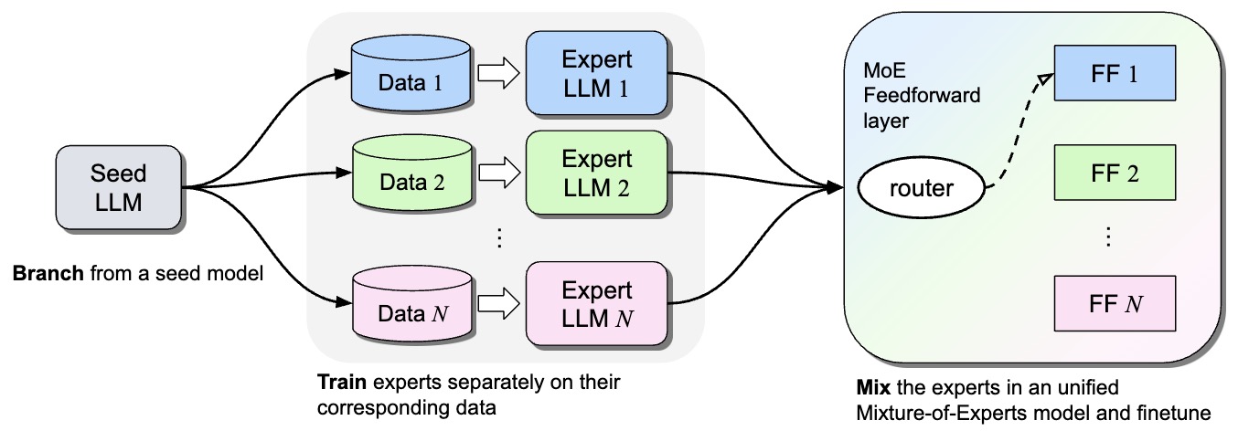
-
Results:
-
BTX outperforms baselines including:
- Llama-2 7B/13B (dense)
- Branch-Train-Merge (BTM)
- Sparse Upcycling (MoE from duplicated seed FF layers)
- Specialists like Llemma and CodeLlama in multi-domain performance.
-
On benchmarks (GSM8K, MATH, HumanEval, MBPP, Natural Questions, MMLU):
- BTX-Top2 achieves best average score (47.9), matching or exceeding specialists in their domains while maintaining generalist performance.
- BTX surpasses Llama-2 13B in all domains except reasoning, despite using half the compute.
-
-
Empirical Findings:
- Routing Analysis: Load balancing during MoE finetuning ensures even usage of experts and avoids dead experts (especially Code expert).
- Efficiency: In compute-matched settings, BTX trains on >2× data than Sparse Upcycling and achieves better generalization.
-
Ablations:
- Blending experts harms performance.
- Freezing expert FF modules during MoE finetuning has minimal impact, indicating pretrained domain knowledge suffices.
- Sample Top-1 routing offers better compute-performance tradeoffs than Switch or Soft routing.
SwitchHead: Accelerating Transformers with Mixture-of-Experts Attention
-
This paper by Csordás et al. introduces SwitchHead, a novel MoE architecture designed specifically for the attention layer in Transformers, a direction underexplored in prior work where MoE has largely been applied only to the feedforward components (MLPs). SwitchHead significantly reduces computational and memory overhead, while maintaining or exceeding the performance of dense, parameter-matched Transformer baselines.
-
Core Idea: Unlike prior attempts at MoE in attention (e.g., MoA), SwitchHead reduces the number of attention matrices by computing MoE projections outside the attention core. It conditionally applies expert selection to value and output projections only, keeping query and key projections fixed per head. This design enables up to 8x fewer attention computations without harming model expressiveness or performance.
-
Architecture and Implementation:
-
Redefinition of Head: A “head” in SwitchHead is redefined as an instance of an attention matrix computation. Each head has its own set of value and output experts (E experts per head).
-
Expert Routing:
- Uses non-competitive sigmoid gating (σ-MoE style).
- Selection is done independently for source (value) and destination (output) projections.
- For a given head \(h\), the value projection is: \(V^h = \sum_{e \in E^h_S} s^h_S[e] \cdot xW^{h,e}_V\)
- The final output is: \(y = \sum_h \sum_{e \in E^h_D} s^h_D[e] \cdot A^h V^h W^{h,e}_O\)
-
Training:
- No special regularization or tricks are required (unlike softmax-gated MoEs).
- All models are trained for 100k steps using Adam with standard learning rates and dropout.
- Language modeling tasks are evaluated under both parameter-matched and MAC-matched settings.
-
Model Configuration:
- Uses 2 or 4 heads, each with multiple experts (typically 4–5).
- Expert selection budget \(k\) (number of active experts) ranges from 2–4.
- Transformer XL and RoPE positional encodings are supported.
-
Datasets: C4, Wikitext-103, Enwik8, and peS2o for pretraining; Lambada, BLiMP, and CBT for zero-shot downstream evaluation.
-
Performance Comparison:
- In parameter-matched settings, SwitchHead achieves similar perplexity with only 44% compute and 27% memory usage.
- In MAC-matched settings, it outperforms the baseline in both perplexity and zero-shot accuracy.
- Compared to Mixture of Attention Heads (MoA), SwitchHead is more compute-efficient due to fewer attention matrices and avoids competitive gating complexities.
-
SwitchAll: Combines SwitchHead attention with σ-MoE-based MLPs for a fully MoE Transformer. Demonstrates further reductions in compute and memory with no degradation in language modeling performance.
-
Analysis:
- SwitchHead’s attention maps are qualitatively similar to dense Transformers, including interpretable induction heads.
- Attention head usage is sparse and often semantically specialized.
-
Key Empirical Finding:
- MoE for value and output projections is essential; MoE for key and query projections offers no benefit under parameter-matching.
-
The following figure from the paper shows a schematic representation of SwitchHead. It consists of a few independent heads, each with multiple experts for value and output projections. Each head has a single attention matrix.
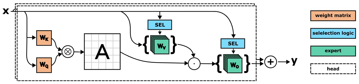
-
-
Benchmarks:
- On Wikitext-103, a 47M SwitchHead matches the baseline (perplexity ~12.3) with 62% fewer MACs and 77% less memory usage.
- On downstream tasks (Lambada, BLiMP, CBT), SwitchHead outperforms dense baselines in zero-shot accuracy.
UMoE: Unifying Attention and FFN with Shared Experts
-
This paper by Yang et al. introduces UMoE, a novel MoE architecture that unifies attention and feed-forward network (FFN) layers in Transformer models. The core innovation lies in reformulating attention mechanisms to reveal an FFN-like structure, enabling shared expert design and efficient parameter sharing across both attention and FFN modules. This approach enhances performance while maintaining computational efficiency and model scalability.
-
Traditional sparse MoE models apply expert selection only in FFN layers due to structural simplicity. Attempts to extend MoE to attention layers face challenges related to complex attention operations and expert routing. UMoE addresses these challenges by decomposing attention into token mixing followed by expert processing, thus aligning attention with the structure of FFN layers.
-
Architecture and Implementation:
-
Pre-mixing Attention Reformulation: The authors reinterpret multi-head attention to highlight a two-step process:
- First, perform token mixing (contextualization) using softmax attention over keys and values.
- Then apply expert processing via two consecutive matrix multiplications—mirroring the FFN structure.
- Expert outputs are then aggregated using weighted attention scores.
-
Expert Design:
- Experts are two-layer MLPs (with non-linearity), sized similarly to FFN modules but configured with reduced intermediate dimension \(d_v\).
- Experts are shared across both attention and FFN layers, reducing parameter redundancy.
- To mitigate parameter bloat due to unique query projections per expert, low-rank parameterization (LoRA-style) is used: \(q_i = xW_q + xW_a^{(i)}W_b^{(i)}\)
-
Routing Mechanism:
- A top-k router selects the most relevant experts for each token.
- In attention modules, all tokens share key/value matrices, while each expert contributes uniquely parameterized query projections.
- In FFN layers, each token is processed independently by its top-k selected experts.
-
UMoE Layer Structure:
- Incorporates pre-mixing attention followed by FFN, with shared experts used in both parts.
- Attention experts operate on token-mixed (contextual) inputs; FFN experts operate on independent tokens.
- The design generalizes FFN-MoE as a special case of attention-MoE with identity attention weights.
-
Training and Optimization:
- UMoE uses decoder-only Transformer blocks with rotary embeddings.
- Incorporates Switch Transformer’s load balancing loss to encourage even expert utilization.
- Models are trained on FineWeb-Edu (100B tokens) and Wikitext-103 (100M tokens) using standard setups (12-layer 134M and 24-layer 1.1B models).
-
The following figure from the paper shows (;eft) the architecture of a UMoE layer, incorporating MoE into both FFN and attention modules with shared experts. The primary distinction between attention-MoE and FFN-MoE lies in an additional token mixing operation; (right) Two formulations of the multi-head attention mechanism. (a) Vanilla attention interleaves mixing operations with value and output projections. (b) Pre-mixing attention performs token mixing prior to projections.
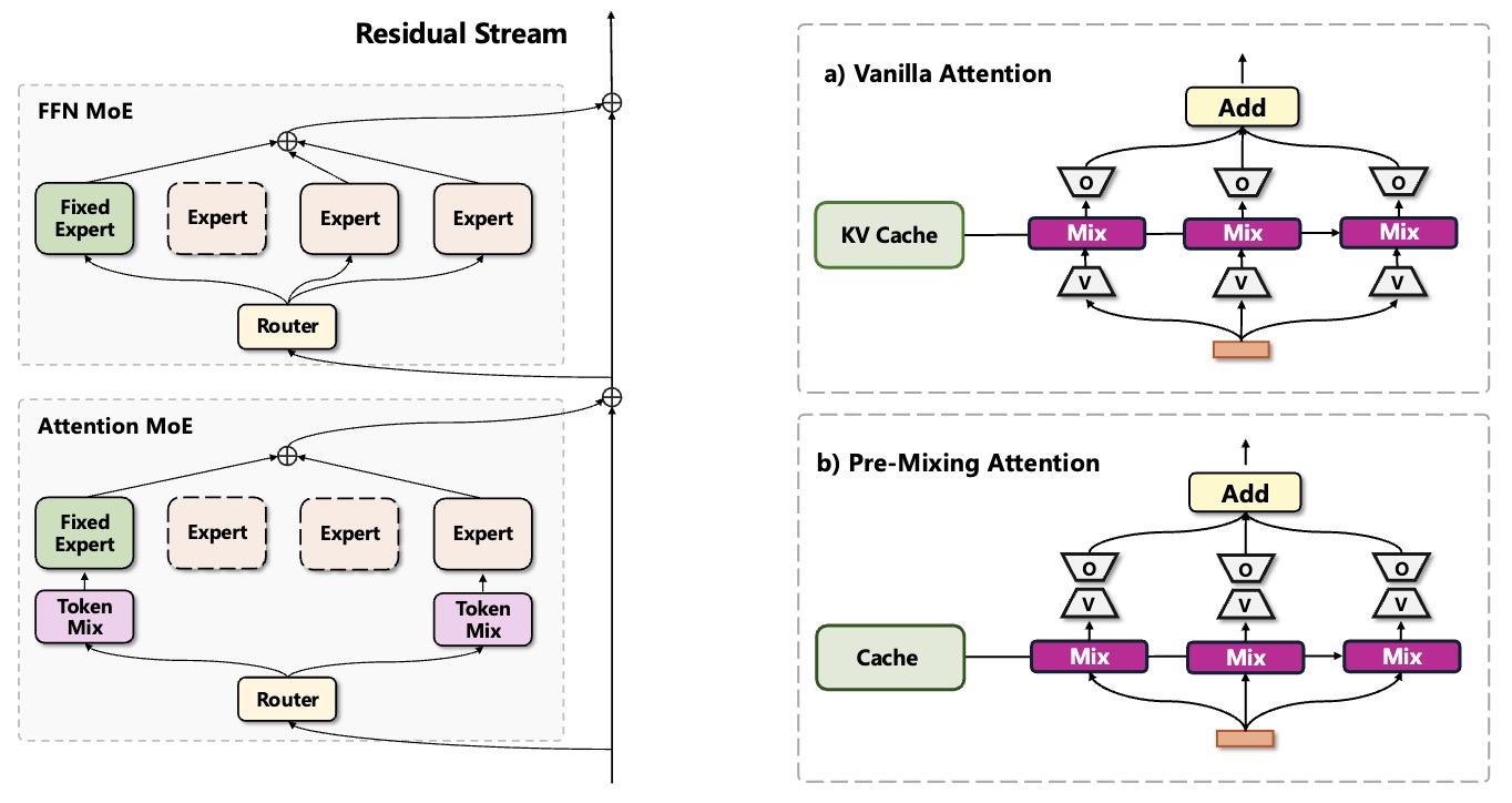
-
-
Empirical Results:
- On both pretraining (perplexity) and zero-shot downstream tasks, UMoE consistently outperforms dense, FFN-MoE, and prior attention-MoE baselines (e.g., MoA, SwitchHead).
- Zero-shot accuracy improvements are observed on benchmarks like MMLU, ARC, RACE, and HellaSwag.
- MAC-matched comparisons show UMoE retains its edge even when other models are given equivalent compute budgets.
- Inference efficiency: While introducing ~1.17× latency at smaller scales, UMoE’s overhead drops to ~1.03× in large models due to amortized compute in expert layers.
-
Ablation Studies and Analysis:
- Pre-mixing vs. Post-mixing: Pre-mixing (contextual input → expert) significantly outperforms post-mixing (expert output → attention) in both training speed and final performance.
- Expert Allocation: Allocating more experts to attention layers rather than FFNs improves performance, reinforcing the theoretical equivalence of FFNs as limited-attention layers.
- Activation Functions: Including activation between expert matrix layers boosts performance; removing them leads to consistent degradation, highlighting the role of non-linearity.
- Expert Specialization: Routing analysis shows interpretable specialization patterns (e.g., determiners or punctuation tokens routing to specific experts across layers).
Mixture of Attention Heads: Selecting Attention Heads Per Token
-
This paper by Zhang et al. from Beihang University, Mila, and Tencent introduces the Mixture of Attention Heads (MoA), a novel attention mechanism that integrates the MoE framework into the multi-head attention (MHA) component of Transformer architectures. While previous MoE work mainly focused on feedforward layers, MoA innovatively applies conditional computation to attention heads, allowing different tokens to dynamically select specialized attention heads, thereby improving performance and computational efficiency.
-
Core Architecture and Computation:
-
Model Composition: MoA replaces the standard MHA with a structure containing:
- A routing network that assigns confidence scores to each attention head (called attention experts).
- A set of attention experts, each with its own query and output projection weights but shared key and value projections to reduce redundancy.
-
Token-specific Selection: For each input token, the routing network selects the top-\(k\) attention experts based on softmax-normalized scores derived from a linear projection of the query. The selected heads’ outputs are weighted by their routing confidence and summed to produce the token-level output:
\[y_t = \sum_{i \in G(q_t)} w_{i,t} \cdot E_i(q_t, K, V)\] -
Expert Attention Computation:
- Each expert performs scaled dot-product attention using its own \(W^q_i\) and \(W^o_i\), while sharing \(W^k\) and \(W^v\) across all experts.
- Output per expert: \(E_i(q_t, K, V) = \text{Softmax}\left(\frac{q_t W^q_i (K W^k)^T}{\sqrt{d_h}}\right) V W^v W^o_i\)
-
Training Losses:
- Auxiliary Load Balancing Loss \(L_a\) to promote expert usage diversity:
\(L_a(Q) = N \cdot \sum_{i=1}^{N} f_i \cdot P_i\)
- where \(f_i\) counts token assignments and \(P_i\) is the aggregated routing probability for expert \(i\).
- Router Z-loss \(L_z\) stabilizes training by penalizing large pre-softmax logits: \(L_z(x) = \frac{1}{T} \sum_{j=1}^T \left(\log \sum_{t=1}^N e^{x_{i,t}} \right)^2\)
- Total training loss:
\(L = L_\text{model} + \sum_{\text{MoA modules}} \left(\alpha L_a + \beta L_z\right)\)
- with default hyperparameters \(\alpha = 0.01\), \(\beta = 0.001\).
- Auxiliary Load Balancing Loss \(L_a\) to promote expert usage diversity:
\(L_a(Q) = N \cdot \sum_{i=1}^{N} f_i \cdot P_i\)
-
Efficiency:
- MoA can scale to more attention heads with only modest increases in memory/computation.
- Computation and parameter complexity are reduced relative to standard MHA when \(k d_h \approx d_m\).
-
The following figure from the paper shows the MoA architecture: attention heads are grouped as experts, each token routes to a top-\(k\) subset, and final outputs are a weighted sum of selected experts’ outputs.
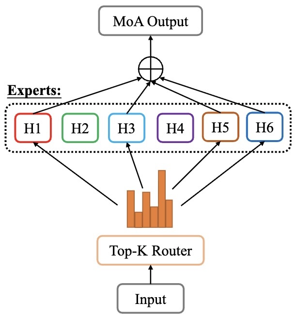
-
-
Experimental Results:
-
Machine Translation:
- Benchmarked on WMT14 En-De and En-Fr with BLEU scores.
- MoA-base (8K8E128D) outperforms Transformer-base (28.4 vs. 27.3 BLEU) and matches or beats deeper models with less computation.
- MoA-big (16K32E256D) achieves near-SOTA with fewer MACs (e.g., 43.7 BLEU vs. Admin-60L-12L’s 43.8, but with less than half the MACs).
-
Masked Language Modeling:
- Evaluated on WikiText-103 using perplexity (PPL).
- MoA models consistently outperform standard Transformers, with performance improving as number of experts and head dimensions increase, while keeping computational cost nearly fixed.
-
-
Interpretability and Analysis:
- MoA allows analysis of expert load balancing—experts receive diverse token subsets, with usage roughly balanced.
- Specialization emerges among experts; PMI analysis reveals certain experts correlate strongly with specific semantic classes (e.g., locations, tech terms, names), indicating improved model interpretability.
-
Implementation Details:
- Uses pre-computed shared \(K, V\) projections for all experts.
- Trained with Adam optimizer and inverse square root scheduler.
- Evaluated using standard benchmarks and MACs (Multiply–Accumulate Operations) for computational cost.
-
Scalability and Efficiency:
- MoA is highly scalable in terms of the number of experts without proportionally increasing compute.
- Ablation studies confirm the value of auxiliary losses for load balancing and performance.
- Despite low theoretical compute, implementation needs CUDA-level optimization for faster wall-clock execution.
Further Reading
Citation
If you found our work useful, please cite it as:
@article{Chadha2020DistilledLossFunctions,
  title   = {Loss Functions},
  author  = {Chadha, Aman and Jain, Vinija},
  journal = {Distilled AI},
  year    = {2020},
  note    = {\url{https://vinija.ai}}
}