Aman's AI Journal • Interview Questions
- Deep Learning
- What are some drawbacks of the Transformer?
- Why do we initialize weights randomly? / What if we initialize the weights with the same values?
- Describe learning rate schedule/annealing.
- Explain mean/average in terms of attention.
- What is convergence in k-means clustering?
- List some debug steps/reasons for your ML model underperforming on the test data
- Popular machine learning models: Pros and Cons
- Define correlation
- What is a Correlation Coefficient?
- Explain Pearson’s Correlation Coefficient
- Explain Spearman’s Correlation Coefficient
- Compare Pearson and Spearman coefficients
- How to choose between Pearson and Spearman correlation?
- Explain the central limit theorem and give examples of when you can use it in a real-world problem?
- Describe the motivation behind random forests and mention two reasons why they are better than individual decision trees?
- Mention three ways to make your model robust to outliers?
- Given two arrays, write a python function to return the intersection of the two. For example, X = [1,5,9,0] and Y = [3,0,2,9] it should return [9,0]
- Given an array, find all the duplicates in this array for example: input: [1,2,3,1,3,6,5] output: [1,3]
- What are the differences and similarities between gradient boosting and random forest? and what are the advantage and disadvantages of each when compared to each other?
- Small file and big file problem in big data
- What are L1 and L2 regularization? What are the differences between the two?
- What are the Bias and Variance in a Machine Learning Model and explain the bias-variance trade-off?
- Briefly explain the A/B testing and its application? What are some common pitfalls encountered in A/B testing?
- Mention three ways to handle missing or corrupted data in adataset?
- How do you avoid #overfitting? Try one (or more) of the following:
- Data science /#MLinterview are hard - regardless which side of the table you are on.
- Order of execution of an SQL Query in Detail
- Explain briefly the logistic regression model and state an example of when you have used it recently?
- Describe briefly the hypothesis testing and p-value in layman’s terms? And give a practical application for them?
- What is an activation function and discuss the use of an activation function? Explain three different types of activation functions?
- If you roll a dice three times, what is the probability to get two consecutive threes?
- You and your friend are playing a game with a fair coin. The two of you will continue to toss the coin until the sequence HH or TH shows up. If HH shows up first, you win, and if TH shows up first your friend win. What is the probability of you winning the game?
- Dimensionality reduction techniques
- Active learning
- What is the independence assumption for a Naive Bayes classifier?
- What are the applications of Bayes’ Theorem?
- Explain briefly batch gradient descent, stochastic gradient descent, and mini-batch gradient descent? List the pros and cons of each.
- Explain what is information gain and entropy in the context of decision trees?
- What are some applications of RL beyond gaming and self-driving cars?
- You are using a deep neural network for a prediction task. After training your model, you notice that it is strongly overfitting the training set and that the performance on the test isn’t good. What can you do to reduce overfitting?
- Explain the linear regression model and discuss its assumption?
- Explain briefly the K-Means clustering and how can we find the best value of K?
- Given an integer array, return the maximum product of any three numbers in the array.
- What are joins in SQL and discuss its types?
- Why should we use Batch Normalization?
- What is weak supervision?
- What is active learning?
- What are the types of active learning?
- What is the difference between online learning and active learning?
- Why is active learning not frequently used with deep learning?
- What does active learning have to do with explore-exploit?
- What are the differences between a model that minimizes squared error and the one that minimizes the absolute error? and in which cases each error metric would be more appropriate?
- Define tuples and lists in Python What are the major differences between them?
- Given a left-skewed distribution that has a median of 60, what conclusions can we draw about the mean and the mode of the data?
- Explain the kernel trick in SVM and why we use it and how to choose what kernel to use?
- Can you explain the parameter sharing concept in deep learning?
- What is the difference between BETWEEN and IN operators in SQL?
- What is the meaning of selection bias and how to avoid it?
- Given two python series, write a function to compute the euclidean distance between them?
- Define the cross-validation process and the motivation behind using it?
- What is the difference between the Bernoulli and Binomial distribution?
- Given an integer \(n\) and an integer \(K\), output a list of all of the combinations of \(k\) numbers chosen from 1 to \(n\). For example, if \(n=3\) and \(k=2\), return \([1,2],[1,3],[2,3]\).
- Explain the long-tailed distribution and provide three examples of relevant phenomena that have long tails. Why are they important in classification and regression problems?
- You are building a binary classifier and found that the data is imbalanced, what should you do to handle this situation?
- If there are 30 people in a room, what is the probability that everyone has different birthdays?
- What is the Vanishing Gradient Problem and how do you fix it?
- What are Residual Networks? How do they help with vanishing gradients?
- How does ResNet-50 solve the vanishing gradients problem of VGG-16?
- How do you run a deep learning model efficiently on-device?
- When are tress not useful?
- Gradient descent: Local Minimum vs. Global Minimum
- Why can’t the mean squared error be used for classification?
- What is overfitting? What are some ways to mitigate it?
- How do you mitigate data imbalance during model training?
- Which ensembling methods work well for class imbalance/long tail scenarios?
- What is focal loss? How does it help mitigate class imbalance?
- How do you define uncertainty with regression problems?
- How do we fix distribution shift in machine learning?
- What is self-attention?
- why do we need Q, K and V in self attention?
- What is the difference between DDPM and DDIM models?
- What is the difference between Tree of Thought prompting and Chain of Thought prompting? Which is better and why?
- What is mode collapse in GANs?
- What loss functions are generally used in GANs?
- What are some transformer-specific regularization methods?
- What are transformer specific normalization methods?
- What is curriculum training? What does it do to the loss surface?
- What are types of ensemble models? Why do they perform better than regular models?
- Why should you make inductive biases in models? What can’t we consider the whole search space?
- How do you identify if a model is hallucinating? What are some mitigation strategies?
- Why were RNNs introduced? How are LSTMs different and what issue do they solve?
- What is the need for DL models? Explain traditional ML models and cases where they would fail?
- In self-attention, why do we use projections of K,Q,V instead of the original values?
- What does the “stable” in stable diffusion refer to?
- What are some automated ways to evaluate the quality of LLM generated output without reference data?
- How do you avoid saddle points during optimization?
- When do you use Bayesian optimization? Can you explain how it works?
- What is the difference between auto-encoder (AE) and variational auto-encoder (VAE)? What do we include in the loss function of the VAE to enforce its properties?
- The cross entropy loss function is non-convex when used in complex deep neural networks. Yet, this is rarely a problem despite the high likelihood of ending up in a local minimum. Why?
- How would you make a GCN (Graph Convolutional Neural Network) behave like a Transformer (or simulate a Transformer)?
- Explain how LoRA works.
- What is the difficulty with using the natural gradient (second order gradient) in optimisation rather than the regular gradient descent family (first order)?
- In the past, CNNs were used for translation. Explain why they are not anymore?
- Why in Transformers positional encodings are used whereas no such mechanisms are used in RNNs or CNNs. Follow- up: why don’t we use an incremental positional encoding to inform about the positions (1, 2, 3, 4, 5,….), and why do we use sinusoidal functions instead?
- In diffusion models, there is a forward diffusion process, and a denoising process. For these two processes, when do you use them in training and inference?
- At a high level, how do diffusion models work? What are some other models that are useful for image generation, and how do they compare to diffusion models?
- What are the loss functions used in Diffusion Models?
- What is the Denoising Score Matching Loss in Diffusion models? Provide equation and intuition.
- At a high level, what is RLHF? Why is this a novel paradigm compared to, for example, self-supervised learning on an uncurated text corpus? What does alignment mean in the context of LLMs?
- Can you please describe the structure of CNNs? The different layers, activation functions? What are some key properties of activation functions?
- What are some differences between a CNN and a FCNN? Layers and activation functions? Why are they structured differently?
- What are some differences between a CNN and a FFNN? Layers and activation functions? Why are they structured differently?
- Imagine you are designing a CNN from scratch. How would you think about choosing the CNN kernel size? What are some considerations?
- Both a fully-connected layer and a self-attention layer allow for all-to-all interactions. What is the advantage of a self-attention layer?
- What is the advantage of using a self-attention-based ViT model compared to using fully CNN layers?
- What is self-supervised learning? Can you give some examples of self-supervised learning paradigms?
- Did the original Transformer use absolute or relative positional encoding?
- How does the choice of positional encoding method can influence the number of parameters added to the model? Consinder absolute, relative, and rotary positional encoding mechanisms.
- In LLMs, why is RoPE required for context length extension?
- Is multicollinearity and correlation the same?
- Do you need a non-linearity such as ReLU or sigmoid at the last layer of a neural network?
- Explain the concept of temperature in deep learning?
- What is the difference between logits, soft and hard targets?
- What is Deep Learning and How is it Different from Traditional Machine Learning?
- How Does Backpropagation Work in a Neural Network?
- Why Do We Prefer Training on Mini-Batches Rather Than Individual Samples in Deep Learning?
- What are the Benefits of Using Batch Normalization?
- What is Entropy in Information Theory?
- Why is Logistic Regression Considered a Linear Classifier Despite Using the Non-Linear Sigmoid Function?
- How Do You Handle Overfitting in Deep Learning Models?
- Can You Explain the Concept of Convolutional Neural Networks (CNN)?
- How Do You Handle Missing Data in Deep Learning?
- Can You Explain the Concept of Transfer Learning in Deep Learning?
- What is Gradient Descent in Deep Learning?
- What is Representation Learning?
- Explain Label Smoothing
- Please Explain What is Dropout in Deep Learning
- What are Autoencoders?
- Can You Explain the Concept of Attention Mechanism in Deep Learning?
- What are Generative Adversarial Networks (GANs)?
- Can You Explain the Concept of Memory Networks in Deep Learning?
- Explain Capsule Networks in Deep Learning
- Can You Explain the Concept of Generative Models in Deep Learning?
- What is the Concept of Adversarial Training in Deep Learning?
- What is Weight Initialization in Deep Learning?
- Explain Data Augmentation
- What is the Difference Between Standardization and Normalization?
- Is it Possible that During ML Training, Both Validation (or Test) Loss and Accuracy are Increasing?
- Is K-means Clustering Algorithm Guaranteed to Converge with a Unique Result?
- In K-means Clustering, Is it Possible that a Centroid Has No Data Points Assigned to It?
- What is Entropy in Information Theory?
- What is the Difference Between Supervised and Unsupervised Learning?
- How Do You Evaluate the Performance of a Machine Learning Model?
- What is Overfitting in Machine Learning and How Can it be Prevented?
- What is the Difference Between a Decision Tree and Random Forest?
- What is the Bias-Variance Trade-off in Machine Learning?
- What is the Difference Between Batch and Online Learning?
- What is the Difference Between a Decision Boundary and a Decision Surface in Machine Learning?
- What is the use of principal component analysis (PCA) in machine learning?
- What is the use of the Random Forest algorithm in machine learning?
- What is the difference between a generative model and a discriminative model?
- What is the difference between an autoencoder and a variational autoencoder?
- What is Expectation-Maximization (EM) algorithm?
- What is the difference between L1 and L2 regularization in machine learning?
- Explain Support Vector Machine (SVM).
- What is the use of the k-nearest neighbors (k-NN) algorithm?
- What is the use of the Random Sampling method for feature selection in machine learning?
- Explain Bagging method in ensemble learning?
- Explain AdaBoost method in ensemble learning?
- Explain Gradient Boosting method in ensemble learning?
- Explain XGBoost method in ensemble learning?
- NLP
- What are the different types of reasoning tasks in NLP?
- How much VRAM is required to load a 7B LLM?
- What are word embeddings in NLP?
- What is Sentence Encoding?
- Explain the concept of attention mechanism in NLP?
- What are transformer models in NLP?
- Can you explain the concept of Named Entity Recognition (NER) in NLP?
- Explain Part-of-Speech (POS) tagging in NLP?
- Can you explain the concept of Language Modeling in NLP?
- Can you explain the concept of Text Summarization?
- What is Sentiment Analysis?
- Can you explain the concept of Dependency Parsing?
- Explain the Coreference Resolution task in NLP?
- Explain Stemming and Lemmatization in NLP?
- What is Text Classification?
- What are Dialogue Systems in NLP?
- Please explain the concept of Text Generation?
- Can you explain the concept of Text Similarity in NLP?
- Please explain Text Clustering?
- What is Named Entity Disambiguation (NED)?
- What is the difference between a feedforward neural network and a recurrent neural network?
- Is BERT a Text Generation model?
- What is weight tying in language model?
- What is so special about the special tokens used in different LM tokenizers?
- What are Attention Masks?
- Machine Learning
- Misc
- What is the difference between standardization and normalization?
- When do you standardize or normalize features?
- Explain the advantages of the parquet data format and how you can achieve the best data compression with it?
- What is Redis?
- Pitfalls in Spark data engineering that can hurt your data lake performance
- What are Generative and Discriminative Models?
- What are distance-weighted kNNs? What are the limitation of traditional kNNs?
- How does Kafka work as a Pub-Sub?
- How do you swap two numbers without a temporary variable?
- How would a compiler tackle swap operations in a program?
- How are XOR Filters used? What if you require better performance than Bloom filters?
- What are indexing techniques for NoSQL databases?
- Does DPO for LLM alignment use the Bradley-Terry model? If so, how?
- Are k-Nearest Neighbors and k-means clustering parametric?
- How are code LLMs trained with the “fill-in-the-middle” pre-training task?
- For a RAG pipeline aimed at a code generation use-case, what is typically chunked and retrieved for the RAG aspect?
- For a RAG pipeline aimed at a SQL generation use-case, what is typically chunked and retrieved for the RAG aspect?
- How is logistic regression a linear model if the sigmoid function is non-linear?
- How much memory is needed to serve a Large Language Model (LLM)?
- What is Consistent Hashing in Distributed Systems?
- What are some load balancing algorithms in distributed systems?
- Why is Flash attention needed, and how does it work?
- What is Continuous and dynamic batching?
- How does ColBERT carry out late interaction?
- What are bi- and cross-encoder architectures for retrieval?
- What are the pros and cons of Gradient Boosting Decision Trees?
- Why are GBDTs highly effective with sparse data?
- Why are Gradient Boosting Decision Trees inefficient for Continual/Online Learning?
- Are the top/deep layers of the model closer to the final layer or the first layer?
- In the context of fine-tuning deep neural networks, can increasing the number of layers make the model more prone to overfitting?
- How does adding a component to the loss term prevent overfitting with regularization?
- Does an LLM produce different outputs for the same input across different iterations? If so, how?
- Explain how random seed initialization works with LLMs.
- What is a Seed?
- How to Control the Random Seed in Code
- Explanation of How the Seed Alters Generation
- Practical Example: Changing Seed for Diverse Outputs
- Why This Matters
- How does the seed impact the LLM sampling using transformers library?
- What does it mean for an ML model to be non-parametric?
- Which ML algorithms are non-parametric?
- Is k-means clustering parametric?
- What are alpha experiments for feature selection in ML model training?
- Single-Feature Testing
- Correlation Analysis
- Forward and Backward Selection
- PCA and Other Dimensionality Reduction Techniques
- Recursive Feature Elimination (RFE)
- Univariate Feature Selection
- Feature Importance with Tree-Based Models
- Regularization Techniques (L1 and L2)
- Permutation Feature Importance
- Synthetic Feature Generation and Interaction Testing
- Feature Selection Based on Stability Scores
- Best Practices for Alpha Feature Selection Experiments
- What are beta experiments in ML model training?
- Is low bias and variance desirable? What is the Bias-Variance Tradeoff?
- Is high precision and recall desirable? What is the precision-recall tradeoff?
- What is the Zipf’s law (i.e., Power law)?
- What are the most common methods to deal with vanishing gradients?
- What are the most common methods to deal with exploding gradients?
- Are Variational Autoencoders (VAEs) and Autoencoders (AEs) typically non-linear?
- What is the relationship between LDA and VAE in terms of representing the latent space as a distribution rather than a fixed vector?
- When do you use Cohen’s Kappa v/s Kripendorff’s Alpha?
- References
- Citation
Deep Learning
What are some drawbacks of the Transformer?
- The runtime of Transformer architecture is quadratic in the length of the input sequence, which means it can be slow when processing long documents or taking characters as inputs. In other words, computing all pairs of interactions during self-attention means our computation grows quadratically with the sequence length, i.e., \(O(T^2 d)\), where \(T\) is the sequence length, and \(d\) is the dimensionality. Note that for recurrent models, it only grew linearly!
- Say, \(d = 1000\). So, for a single (shortish) sentence, \(T \leq 30 \Rightarrow T^{2} \leq 900 \Rightarrow T^2 d \approx 900K\). Note that in practice, we set a bound such as \(T=512\). Imagine working on long documents with \(T \geq 10,000\)!?
- Wouldn’t it be nice for Transformers if we didn’t have to compute pair-wise interactions between each word pair in the sentence? Recent studies such as:
- Synthesizer: Rethinking Self-Attention in Transformer Models
- Linformer: Self-Attention with Linear Complexity
- Rethinking Attention with Performers
- Big Bird: Transformers for Longer Sequences
- … show that decent performance levels can be achieved without computing interactions between all word-pairs (such as by approximating pair-wise attention).
- Compared to CNNs, the data appetite of transformers is obscenely high. CNNs are still sample efficient, which makes them great candidates for low-resource tasks. This is especially true for image/video generation tasks where an exceptionally large amount of data is needed, even for CNN architectures (and thus implies that Transformer architectures would have a ridiculously high data requirement). For example, the recent CLIP architecture by Radford et al. was trained with CNN-based ResNets as vision backbones (and not a ViT-like transformer architecture). While transformers do offer accuracy bumps once their data requirement is satisfied, CNNs offer a way to deliver decent accuracy performance in tasks where the amount of data available is not exceptionally high. Both architectures thus have their usecases.
- The runtime of the Transformer architecture is quadratic in the length of the input sequence. Computing attention over all word-pairs requires the number of edges in the graph to scale quadratically with the number of nodes, i.e., in an \(n\) word sentence, a Transformer would be doing computations over \(n^{2}\) pairs of words. This implies a large parameter count (implying high memory footprint) and thereby high computational complexity. More in the section on What Would We Like to Fix about the Transformer?
- High compute requirements has a negative impact on power and battery life requirements, especially for portable device targets.
- Overall, a transformer requires higher computational power, more data, power/battery life, and memory footprint, for it to offer better performance (in terms of say, accuracy) compared to its conventional competitors.
Why do we initialize weights randomly? / What if we initialize the weights with the same values?
- If all weights are initialized with the same values, all neurons in each layer give you the same outputs (and thus redundantly learn the same features) which implies the model will never learn. This is the reason that the weights are initialized with random numbers.
- Detailed explanation:
- The optimization algorithms we usually use for training neural networks are deterministic. Gradient descent, the most basic algorithm, that is a base for the more complicated ones, is defined in terms of partial derivatives
-
A partial derivative tells you how does the change of the optimized function is affected by the \(\theta_j\) parameter. If all the parameters are the same, they all have the same impact on the result, so will change by the same quantity. If you change all the parameters by the same value, they will keep being the same. In such a case, each neuron will be doing the same thing, they will be redundant and there would be no point in having multiple neurons. There is no point in wasting your compute repeating exactly the same operations multiple times. In other words, the model does not learn because error is propagated back through the weights in proportion to the values of the weights. This means that all hidden units connected directly to the output units will get identical error signals, and, since the weight changes depend on the error signals, the weights from those units to the output units will be the same.
-
When you initialize the neurons randomly, each of them will hopefully be evolving during the optimization in a different “direction”, they will be learning to detect different features from the data. You can think of early layers as of doing automatic feature engineering for you, by transforming the data, that are used by the final layer of the network. If all the learned features are the same, it would be a wasted effort.
-
The Lottery Ticket Hypothesis: Training Pruned Neural Networks by Frankle and Carbin explores the hypothesis that the big neural networks are so effective because randomly initializing multiple parameters helps our luck by drawing the lucky “lottery ticket” parameters that work well for the problem.
Describe learning rate schedule/annealing.
- Am optimizer is typically used with a learning rate schedule that involves a short warmup phase, a constant hold phase and an exponential decay phase. The decay/annealing is typically done using a cosine learning rate schedule over a number of cycles (Loshchilov & Hutter, 2016).
Explain mean/average in terms of attention.
- Averaging is equivalent to uniform attention.
What is convergence in k-means clustering?
- In case of \(k\)-means clustering, the word convergence means the algorithm has successfully completed clustering or grouping of data points in \(k\) number of clusters. The algorithm determines that it has grouped/clustered the data points into correct clusters if the centroids (\(k\) values) in the last two consequent iterations are same then the algorithm is said to have converged. However, in practice, people often use a less strict criteria for convergence, for e.g., the difference in the values of last two iterations needs to be less than a low threshold.
List some debug steps/reasons for your ML model underperforming on the test data
- Insufficient quantity of training data: Machine learning algorithms need a large amount of data to be able to learn the underlying statistics from the data and work properly. Even for simple problems, the models will typically need thousands of examples.
- Nonrepresentative training data: In order for the model to generalize well, your training data should be representative of what is expected to be seen in the production. If the training data is nonrepresentative of the production data or is different this is known as data mismatch.
- Poor quality data: Since the learning models will use the data to learn the underlying pattern and statistics from it. It is critical that the data are rich in information and be of good quality. Having training data that are full of outliers, errors, noise, and missing data will decrease the ability of the model to learn from data, and then the model will act poorly on new data.
- Irrelevant features: As the famous quote says “garbage in, garbage out”. Your machine learning model will be only able to learn if the data contains relevant features and not too many irrelevant features.
- Overfitting the training data: Overfitting happens when the model is too complex relative to the size of the data and its quality, which will result in learning more about the pattern in the noise of the data or very specific patterns in the data which the model will not be able to generalize for new instances.
- Underfitting the training data: Underfitting is the opposite of overfitting, the model is too simple to learn any of the patterns in the training data. This could be known when the training error is large and also the validation and test error is large.
Popular machine learning models: Pros and Cons
Linear Regression
Pros
- Simple to implement and efficient to train.
- Overfitting can be reduced by regularization.
- Performs well when the dataset is linearly separable.
Cons
- Assumes that the data is independent which is rare in real life.
- Prone to noise and overfitting.
- Sensitive to outliers.
Logistic Regression
Pros
- Less prone to over-fitting but it can overfit in high dimensional datasets.
- Efficient when the dataset has features that are linearly separable.
- Easy to implement and efficient to train.
Cons
- Should not be used when the number of observations are lesser than the number of features.
- Assumption of linearity which is rare in practice.
- Can only be used to predict discrete functions.
Support Vector Machines
Pros
- Good at high dimensional data.
- Can work on small dataset.
- Can solve non-linear problems.
Cons
- Inefficient on large data.
- Requires picking the right kernel.
Decision Trees
- Decision Trees can be used for both classification and regression.
- For classification, you can simply return the majority vote of the trees.
- For regression, you can return the averaged values of the trees.
Pros
- Can solve non-linear problems.
- Can work on high-dimensional data with excellent accuracy.
- Easy to visualize and explain.
Cons
- Overfitting. Might be resolved by random forest.
- A small change in the data can lead to a large change in the structure of the optimal decision tree.
- Calculations can get very complex.
k-Nearest Neighbor
- k-Nearest Neighbor (kNN) can be used for both classification and regression.
- For classification, you can simply return the majority vote of the nearest neighbors.
- For regression, you can return the averaged values of the nearest neighbors.
Pros
- Can make predictions without training.
- Time complexity is \(O(n)\).
- Can be used for both classification and regression.
Cons
- Does not work well with large dataset.
- Sensitive to noisy data, missing values and outliers.
- Need feature scaling.
- Choose the correct \(K\) value.
k-Means Clustering
- k-Means Clustering (kMC) is a classifier.
Pros
- Simple to implement.
- Scales to large data sets.
- Guarantees convergence.
- Easily adapts to new examples.
- Generalizes to clusters of different shapes and sizes.
Cons
- Sensitive to the outliers.
- Choosing the k values manually is tough.
- Dependent on initial values.
- Scalability decreases when dimension increases.
Principal Component Analysis
- Principal Component Analysis (PCA) is a dimensionality reduction technique that reduces correlated (features that show co-variance) features and projects them to a lower-dimensional space.
Pros
- Reduce correlated features.
- Improve performance.
- Reduce overfitting.
Cons
- Principal components are less interpretable.
- Information loss.
- Must standardize data before implementing PCA.
Naive Bayes
Pros
- Training period is less.
- Better suited for categorical inputs.
- Easy to implement.
Cons
- Assumes that all features are independent which is rarely happening in real life.
- Zero Frequency.
- Estimations can be wrong in some cases.
ANN
Pros
- Have fault tolerance.
- Have the ability to learn and model non-linear and complex relationships.
- Can generalize on unseen data.
Cons
- Long training time.
- Non-guaranteed convergence.
- Black box. Hard to explain solution.
- Hardware dependence.
- Requires user’s ability to translate the problem.
Adaboost
Pros
- Relatively robust to overfitting.
- High accuracy.
- Easy to understand and to visualize.
Cons
- Sensitive to noise data.
- Affected by outliers.
- Not optimized for speed.
Define correlation
- Correlation is the degree to which two variables are linearly related. This is an important step in bi-variate data analysis. In the broadest sense correlation is actually any statistical relationship, whether causal or not, between two random variables in bivariate data.
An important rule to remember is that correlation doesn’t imply causation.
- Let’s understand through two examples as to what it actually implies.
- The consumption of ice-cream increases during the summer months. There is a strong correlation between the sales of ice-cream units. In this particular example, we see there is a causal relationship also as the extreme summers do push the sale of ice-creams up.
- Ice-creams sales also have a strong correlation with shark attacks. Now as we can see very clearly here, the shark attacks are most definitely not caused due to ice-creams. So, there is no causation here.
- Hence, we can understand that the correlation doesn’t ALWAYS imply causation!
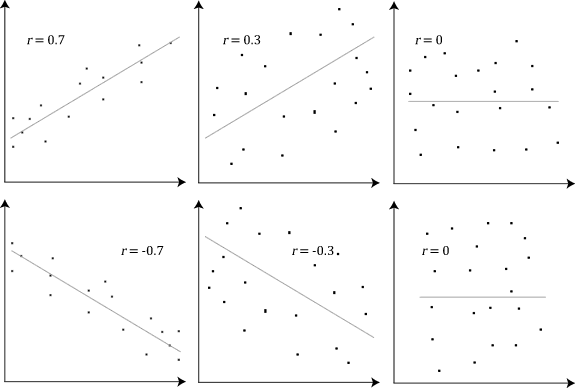
What is a Correlation Coefficient?
- A correlation coefficient is a statistical measure of the strength of the relationship between the relative movements of two variables. The values range between -1.0 and 1.0. A correlation of -1.0 shows a perfect negative correlation, while a correlation of 1.0 shows a perfect positive correlation. A correlation of 0.0 shows no linear relationship between the movement of the two variables.
Explain Pearson’s Correlation Coefficient
-
Wikipedia Definition: In statistics, the Pearson correlation coefficient also referred to as Pearson’s r or the bivariate correlation is a statistic that measures the linear correlation between two variables X and Y. It has a value between +1 and −1. A value of +1 is a total positive linear correlation, 0 is no linear correlation, and −1 is a total negative linear correlation.
-
Important Inference to keep in mind: The Pearson correlation can evaluate ONLY a linear relationship between two continuous variables (A relationship is linear only when a change in one variable is associated with a proportional change in the other variable)
-
Example use case: We can use the Pearson correlation to evaluate whether an increase in age leads to an increase in blood pressure.
-
Below is an example (source: Wikipedia) of how the Pearson correlation coefficient (r) varies with the strength and the direction of the relationship between the two variables. Note that when no linear relationship could be established (refer to graphs in the third column), the Pearson coefficient yields a value of zero.
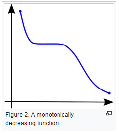
Explain Spearman’s Correlation Coefficient
-
Wikipedia Definition: In statistics, Spearman’s rank correlation coefficient or Spearman’s ρ, named after Charles Spearman is a non-parametric measure of rank correlation (statistical dependence between the rankings of two variables). It assesses how well the relationship between two variables can be described using a monotonic function.
-
Important Inference to keep in mind: The Spearman correlation can evaluate a monotonic relationship between two variables — Continous or Ordinal and it is based on the ranked values for each variable rather than the raw data.
-
What is a monotonic relationship?
- A monotonic relationship is a relationship that does one of the following:
- As the value of one variable increases, so does the value of the other variable, OR,
- As the value of one variable increases, the other variable value decreases.
- But, not exactly at a constant rate whereas in a linear relationship the rate of increase/decrease is constant.
- A monotonic relationship is a relationship that does one of the following:
- Example use case: Whether the order in which employees complete a test exercise is related to the number of months they have been employed or correlation between the IQ of a person with the number of hours spent in front of TV per week.
Compare Pearson and Spearman coefficients
- The fundamental difference between the two correlation coefficients is that the Pearson coefficient works with a linear relationship between the two variables whereas the Spearman Coefficient works with monotonic relationships as well.
- One more difference is that Pearson works with raw data values of the variables whereas Spearman works with rank-ordered variables.
- Now, if we feel that a scatterplot is visually indicating a “might be monotonic, might be linear” relationship, our best bet would be to apply Spearman and not Pearson. No harm would be done by switching to Spearman even if the data turned out to be perfectly linear. But, if it’s not exactly linear and we use Pearson’s coefficient then we’ll miss out on the information that Spearman could capture.
-
Let’s look at some examples (source: A comparison of the Pearson and Spearman correlation methods):
- Pearson = +1, Spearman = +1:
- Pearson = +0.851, Spearman = +1 (This is a monotonically increasing relationship, thus Spearman is exactly 1)
- Pearson = −0.093, Spearman = −0.093
- Pearson = −1, Spearman = −1
- Pearson = −0.799, Spearman = −1 (This is a monotonically decreasing relationship, thus Spearman is exactly 1)
- Note that both of these coefficients cannot capture any other kind of non-linear relationships. Thus, if a scatterplot indicates a relationship that cannot be expressed by a linear or monotonic function, then both of these coefficients must not be used to determine the strength of the relationship between the variables.
How to choose between Pearson and Spearman correlation?
-
If you want to explore your data it is best to compute both, since the relation between the Spearman (S) and Pearson (P) correlations will give some information. Briefly, \(S\) is computed on ranks and so depicts monotonic relationships while \(P\) is on true values and depicts linear relationships.
-
As an example, if you set:
x=(1:100);
y=exp(x);                         % then,
corr(x,y,'type','Spearman');      % will equal 1, and
corr(x,y,'type','Pearson');       % will be about equal to 0.25
- This is because \(y\) increases monotonically with \(x\) so the Spearman correlation is perfect, but not linearly, so the Pearson correlation is imperfect.
corr(x,log(y),'type','Pearson'); % will equal 1
- Doing both is interesting because if you have \(S > P\), that means that you have a correlation that is monotonic but not linear. Since it is good to have linearity in statistics (it is easier) you can try to apply a transformation on \(y\) (such a log).
Explain the central limit theorem and give examples of when you can use it in a real-world problem?
- The center limit theorem states that if any random variable, regardless of the distribution, is sampled a large enough times, the sample mean will be approximately normally distributed. This allows for studying the properties of any statistical distribution as long as there is a large enough sample size.
Describe the motivation behind random forests and mention two reasons why they are better than individual decision trees?
- The motivation behind random forest or ensemble models in general in layman’s terms, Let’s say we have a question/problem to solve we bring 100 people and ask each of them the question/problem and record their solution. Next, we prepare a solution which is a combination/ a mixture of all the solutions provided by these 100 people. We will find that the aggregated solution will be close to the actual solution. This is known as the “Wisdom of the crowd” and this is the motivation behind Random Forests. We take weak learners (ML models) specifically, Decision Trees in the case of Random Forest & aggregate their results to get good predictions by removing dependency on a particular set of features. In regression, we take the mean and for Classification, we take the majority vote of the classifiers.
- A random forest is generally better than a decision tree, however, you should note that no algorithm is better than the other it will always depend on the use case & the dataset [Check the No Free Lunch Theorem in the first comment]. Reasons why random forests allow for stronger prediction than individual decision trees: 1) Decision trees are prone to overfit whereas random forest generalizes better on unseen data as it is using randomness in feature selection as well as during sampling of the data. Therefore, random forests have lower variance compared to that of the decision tree without substantially increasing the error due to bias. 2) Generally, ensemble models like Random Forest perform better as they are aggregations of various models (Decision Trees in the case of Random Forest), using the concept of the “Wisdom of the crowd.”
Mention three ways to make your model robust to outliers?
-
Investigating the outliers is always the first step in understanding how to treat them. After you understand the nature of why the outliers occurred you can apply one of the several methods mentioned below.
-
Add regularization that will reduce variance, for example, L1 or L2 regularization.
-
Use tree-based models (random forest, gradient boosting ) that are generally less affected by outliers.
-
Winsorize the data. Winsorizing or winsorization is the transformation of statistics by limiting extreme values in the statistical data to reduce the effect of possibly spurious outliers. In numerical data, if the distribution is almost normal using the Z-score we can detect the outliers and treat them by either removing or capping them with some value. If the distribution is skewed using IQR we can detect and treat it by again either removing or capping it with some value. In categorical data check for value_count in the percentage if we have very few records from some category, either we can remove it or can cap it with some categorical value like others.
-
Transform the data, for example, you do a log transformation when the response variable follows an exponential distribution or is right-skewed.
-
Use more robust error metrics such as MAE or Huber loss instead of MSE.
-
Remove the outliers, only do this if you are certain that the outliers are true anomalies that are not worth adding to your model. This should be your last consideration since dropping them means losing information.
Given two arrays, write a python function to return the intersection of the two. For example, X = [1,5,9,0] and Y = [3,0,2,9] it should return [9,0]
- A1 (The most repeated one):
set(X).intersect(set(Y))
- A2:
set(X) & set(Y)
-
Using sets is a very good way to do it since it utilizes a hash map implementation underneath it.
-
A3:
def common_func(X, Y):
Z=[]
for i in X:
for j in Y:
if i==j and i not in Z:
Z.append(i)
return Z
- This is also a simple way to do it, however, it leads to the time complexity of O(N*M) so it is better to use sets.
- Some other answers were mentioned that will work for the mentioned case but will return duplicates for other cases, for example, if X = [1,0,9,9] and Y = [3,0,9,9] it will return [0, 9, 9] not [0,9].
A1:
Res=[i for i in x if i in Y]
A2:
Z = [value for value in X if value in Y]
print(Z)
A3:
d = {}
for value in y:
if value not in d:
d[value] = 1
intersection = []
for value in x:
if value in d:
intersection.append(value)

print(intersection)
- The time complexity for this is O(n + m) and the space complexity is O(m), the problem of it is that it returns duplicates.
Given an array, find all the duplicates in this array for example: input: [1,2,3,1,3,6,5] output: [1,3]
- Approach 1:
set1=set()
res=[]
for i in list:
if i in set1:
res.append(i)
else:
set1.add(i)
print(res)
- Approach 2:
arr1=np.array([1,2,3,1,3,6,5])
nums,index,counts=np.unique(arr1,return_index=True,return_counts=True)
print(nums,index,counts)
nums[counts!=1]
- Approach 3:
a=[1,2,3,1,3,6,5]
j=[i for (i,v) in Counter(a).items() if v>1]
Approach 4: Use map (dict), and get the frequency count of each element. Iterate the map, and print all keys whose values are > 1.
What are the differences and similarities between gradient boosting and random forest? and what are the advantage and disadvantages of each when compared to each other?
- Similarities:
- Both these algorithms are decision-tree based algorithms
- Both these algorithms are ensemble algorithms
- Both are flexible models and do not need much data preprocessing.
- Differences:
- Random forests (Uses Bagging): Trees are arranged in a parallel fashion where the results of all trees are aggregated at the end through averaging or majority vote. Every tree is constructed independently of the other trees
- Gradient boosting (Uses Boosting): Trees are arranged in a series sequential fashion where every tree tries to minimize the error of the previous tree. Every tree is dependent on the previous tree.
- Advantages of gradient boosting over random forests:
- Gradient boosting can be more accurate than Random forests because we train them to minimize the previous tree’s error.
- Gradient boosting is capable of capturing complex patterns in the data.
- Gradient boosting is better than random forest when used on unbalanced data sets.
- Advantages of random forests over gradient boosting :
- Random forest is less prone to overfit as compared to gradient boosting.
- Random forest has faster training as trees are created parallelly & independent of each other.
- The disadvantage of GB over RF:
- Gradient boosting is more prone to overfitting than random forests due to their focus on mistakes during training iterations and the lack of independence in tree building.
- If the data is noisy the boosted trees might overfit and start modeling the noise.
- In GB training might take longer because every tree is created sequentially.
- Tuning the hyperparameters of gradient boosting is harder than those of random forest.
Small file and big file problem in big data
- The “small file problem” is kind of notorious in the big data space.
- Did you know there’s also the “Big/large file problem”?
- Say you have a billion records. The small file problem would be like.. 10 records per file and 100 million files. Combining all these files is slow, terrible, and has made many data engineers cry.
- The large file problem would be the opposite problem. 1 billion records in 1 file. This is also a huge problem because how do you parallelize 1 file? You can’t without splitting it up first.
- To avoid crying, the solution is sizing your files the right way. Aiming for between 100-200 MBs for file is usually best. In this contrived example, you’d have a 1000 files each with 1 million records.
- It is worth seeing the spread of files and the size and understanding what optimal file size works out best.
- Too low and you have the risk of more files, too high and the parallelism isn’t going to be effective.
- It is recommended to understand up parallelism, and block size and seeing how the distribution of your data (in files) is before adding an arbitrary default file size value.
What are L1 and L2 regularization? What are the differences between the two?
- Regularization is a technique used to avoid overfitting by trying to make the model more simple. One way to apply regularization is by adding the weights to the loss function. This is done in order to consider minimizing unimportant weights. In L1 regularization we add the sum of the absolute of the weights to the loss function. In L2 regularization we add the sum of the squares of the weights to the loss function.
- So both L1 and L2 regularization are ways to reduce overfitting, but to understand the difference it’s better to know how they are calculated:
- Loss (L2) : Cost function + \(L\) * \(weights^2\)
- Loss (L1) : Cost function + \(L\) * \(\|weights\|\)
- Where \(L\) is the regularization parameter
- L2 regularization penalizes huge parameters preventing any of the single parameters to get too large. But weights never become zeros. It adds parameters square to the loss. Preventing the model from overfitting on any single feature.
- L1 regularization penalizes weights by adding a term to the loss function which is the absolute value of the loss. This leads to it removing small values of the parameters leading in the end to the parameter hitting zero and staying there for the rest of the epochs. Removing this specific variable completely from our calculation. So, It helps in simplifying our model. It is also helpful for feature selection as it shrinks the coefficient to zero which is not significant in the model.
What are the Bias and Variance in a Machine Learning Model and explain the bias-variance trade-off?
-
The goal of any supervised machine learning model is to estimate the mapping function (f) that predicts the target variable (y) given input (x). The prediction error can be broken down into three parts:
-
Bias: The bias is the simplifying assumption made by the model to make the target function easy to learn. Low bias suggests fewer assumptions made about the form of the target function. High bias suggests more assumptions made about the form of the target data. The smaller the bias error the better the model is. If the bias error is high, this means that the model is underfitting the training data.
-
Variance: Variance is the amount that the estimate of the target function will change if different training data was used. The target function is estimated from the training data by a machine learning algorithm, so we should expect the algorithm to have some variance. Ideally, it should not change too much from one training dataset to the next, meaning that the algorithm is good at picking out the hidden underlying mapping between the inputs and the output variables. If the variance error is high this indicates that the model overfits the training data.
-
Irreducible error: It is the error introduced from the chosen framing of the problem and may be caused by factors like unknown variables that influence the mapping of the input variables to the output variable. The irreducible error cannot be reduced regardless of what algorithm is used.
-
-
The goal of any supervised machine learning algorithm is to achieve low bias and low variance. In turn, the algorithm should achieve good prediction performance. The parameterization of machine learning algorithms is often a battle to balance out bias and variance.
- For example, if you want to predict the housing prices given a large set of potential predictors. A model with high bias but low variance, such as linear regression will be easy to implement, but it will oversimplify the problem resulting in high bias and low variance. This high bias and low variance would mean in this context that the predicted house prices are frequently off from the market value, but the value of the variance of these predicted prices is low.
- On the other side, a model with low bias and high variance such as a neural network will lead to predicted house prices closer to the market value, but with predictions varying widely based on the input features.
Briefly explain the A/B testing and its application? What are some common pitfalls encountered in A/B testing?
-
A/B testing helps us to determine whether a change in something will cause a change in performance significantly or not. So in other words you aim to statistically estimate the impact of a given change within your digital product (for example). You measure success and counter metrics on at least 1 treatment vs 1 control group (there can be more than 1 XP group for multivariate tests).
- Applications:
-
Consider the example of a general store that sells bread packets but not butter, for a year. If we want to check whether its sale depends on the butter or not, then suppose the store also sells butter and sales for next year are observed. Now we can determine whether selling butter can significantly increase/decrease or doesn’t affect the sale of bread.
-
While developing the landing page of a website you create 2 different versions of the page. You define a criteria for success eg. conversion rate. Then define your hypothesis,
- Null hypothesis (H): No difference between the performance of the 2 versions.
- Alternative hypothesis (H’): version A will perform better than B.
-
-
Note that you will have to split your traffic randomly (to avoid sample bias) into 2 versions. The split doesn’t have to be symmetric, you just need to set the minimum sample size for each version to avoid undersample bias.
-
Now if version A gives better results than version B, we will still have to statistically prove that results derived from our sample represent the entire population. Now one of the very common tests used to do so is 2 sample t-test where we use values of significance level (alpha) and p-value to see which hypothesis is right. If p-value<alpha, H is rejected.
- Common pitfalls:
- Wrong success metrics inadequate to the business problem
- Lack of counter metric, as you might add friction to the product regardless along with the positive impact
- Sample mismatch: heterogeneous control and treatment, unequal variances
- Underpowered test: too small sample or XP running too short 5. Not accounting for network effects (introduce bias within measurement)
Mention three ways to handle missing or corrupted data in adataset?
-
In general, real-world data often has a lot of missing values. The cause of missing values can be data corruption or failure to record data. The handling of missing data is very important during the preprocessing of the dataset as many machine learning algorithms do not support missing values. However, you should start by asking the data owner/stakeholder about the missing or corrupted data. It might be at the data entry level, because of file encoding, etc. which if aligned, can be handled without the need to use advanced techniques.
-
There are different ways to handle missing data, we will discuss only three of them:
-
Deleting the row with missing values
- The first method to handle missing values is to delete the rows or columns that have null values. This is an easy and fast method and leads to a robust model, however, it will lead to the loss of a lot of information depending on the amount of missing data and can only be applied if the missing data represent a small percentage of the whole dataset.
-
Using learning algorithms that support missing values
- Some machine learning algorithms are robust to missing values in the dataset. The K-NN algorithm can ignore a column from a distance measure when there are missing values. Naive Bayes can also support missing values when making a prediction. Another algorithm that can handle a dataset with missing values or null values is the random forest model and Xgboost (check the post in the first comment), as it can work on non-linear and categorical data. The problem with this method is that these models’ implementation in the scikit-learn library does not support handling missing values, so you will have to implement it yourself.
-
Missing value imputation
- Data imputation means the substitution of estimated values for missing or inconsistent data in your dataset. There are different ways to estimate the values that will replace the missing value. The simplest one is to replace the missing value with the most repeated value in the row or the column. Another simple way is to replace it with the mean, median, or mode of the rest of the row or the column. This advantage of this is that it is an easy and fast way to handle the missing data, but it might lead to data leakage and does not factor the covariance between features. A better way is to use a machine learning model to learn the pattern between the data and predict the missing values, this is a very good method to estimate the missing values that will not lead to data leakage and will factor the covariance between the feature, the drawback of this method is the computational complexity especially if your dataset is large.
-
How do you avoid #overfitting? Try one (or more) of the following:
-
Training with more data, which makes the signal stronger and clearer, and can enable the model to detect the signal better. One way to do this is to use #dataaugmentation strategies
-
Reducing the number of features in order to avoid the curse of dimensionality (which occurs when the amount of data is too low to support highly-dimensional models), which is a common cause for overfitting
-
Using cross-validation. This technique works because the model is unlikely to make the same mistake on multiple different samples, and hence, errors will be evened out
-
Using early stopping to end the training process before the model starts learning the noise
-
Using regularization and minimizing the adjusted loss function. Regularization works because it discourages learning a model that’s overly complex or flexible
-
Using ensemble learning, which ensures that the weaknesses of a model are compensated by the other ones
Data science /#MLinterview are hard - regardless which side of the table you are on.
-
As a jobseeker, it can be really hard to shine, especially when the questions asked have little to no relevance to the actual job. How are you supposed to showcase your ability to build models when the entire interview revolves are binary search trees?
-
As a hiring manager, it’s close to impossible to evaluate modeling skills by just talking to someone, and false positives are really frequent. A question that dramatically reduces the noise on both sides:
“What is the most machine learning complex concept you came across, and how would you explain it to yourself that would have made it easier for you to understand it before you learned it?”
-
The answer will tell you a lot more about the candidate than you might think:
- 90% of candidates answer “overfitting”. If they’re junior and explain it really well and they’re junior, it means they’re detailed-oriented and try to gain a thorough understanding of the field, but they sure could show more ambition; if they don’t, it means their understanding of the fundamentals is extremely basic.
- If they answer back-propagation, and they can explain it well, it means they’re more math-oriented than the average and will probably be a good candidate for a research role as an applied DS role.
- If their answer has something to do with a brand-new ML concept, , and they can explain it well, it means they’re growth-oriented and well-read.
- Generally speaking, if they answer something overly complicated and pompous, but can’t explain it well, it means they’re trying to impress but have an overall shallow understanding - a good rule of thumb is not hire them.
- Now, if you are a candidate, or an ML professional, keep asking yourself that question: “What is the most sophisticated concept, model or architecture you know of?” If you keep giving the same answer, maybe you’ve become complacent, and it’s time for you to learn something new.
- How would you explain it to a newbie? As Einstein said, if “you can’t explain it simply, you don’t understand it well enough”.
Order of execution of an SQL Query in Detail
-
Each query begins with finding the data that we need in a database, and then filtering that data down into something that can be processed and understood as quickly as possible.
-
Because each part of the query is executed sequentially, it’s important to understand the order of execution so that you know what results are accessible where.
-
Consider the below mentioned query :
SELECT DISTINCT column, AGG_FUNC(column_or_expression), …
FROM mytable
JOIN another_table
ON mytable.column = another_table.column
WHERE constraint_expression
GROUP BY column
HAVING constraint_expression
ORDER BY column ASC/DESC
LIMIT count OFFSET COUNT;
- Query order of execution:
1.FROMandJOINs
- TheFROMclause, and subsequentJOINs are first executed to determine the total working set of data that is being queried. This includes subqueries in this clause, and can cause temporary tables to be created under the hood containing all the columns and rows of the tables being joined.
2.WHERE
- Once we have the total working set of data, the first-passWHEREconstraints are applied to the individual rows, and rows that do not satisfy the constraint are discarded. Each of the constraints can only access columns directly from the tables requested in theFROMclause. Aliases in theSELECTpart of the query are not accessible in most databases since they may include expressions dependent on parts of the query that have not yet executed.
3.GROUP BY
- The remaining rows after theWHEREconstraints are applied are then grouped based on common values in the column specified in theGROUP BYclause. As a result of the grouping, there will only be as many rows as there are unique values in that column. Implicitly, this means that you should only need to use this when you have aggregate functions in your query.
4.HAVING
- If the query has aGROUP BYclause, then the constraints in theHAVINGclause are then applied to the grouped rows, discard the grouped rows that don’t satisfy the constraint. Like theWHEREclause, aliases are also not accessible from this step in most databases.
5.SELECT
- Any expressions in theSELECTpart of the query are finally computed.
6.DISTINCT
- Of the remaining rows, rows with duplicate values in the column marked asDISTINCTwill be discarded.
7.ORDER BY
- If an order is specified by theORDER BYclause, the rows are then sorted by the specified data in either ascending or descending order. Since all the expressions in theSELECTpart of the query have been computed, you can reference aliases in this clause.
8.LIMIT/OFFSET
- Finally, the rows that fall outside the range specified by theLIMITandOFFSETare discarded, leaving the final set of rows to be returned from the query.
Explain briefly the logistic regression model and state an example of when you have used it recently?
- Logistic regression is used to calculate the probability of occurrence of an event in the form of a dependent output variable based on independent input variables. Logistic regression is commonly used to estimate the probability that an instance belongs to a particular class. If the probability is bigger than 0.5 then it will belong to that class (positive) and if it is below 0.5 it will belong to the other class. This will make it a binary classifier.
- It is important to remember that the Logistic regression isn’t a classification model, it’s an ordinary type of regression algorithm, and it was developed and used before machine learning, but it can be used in classification when we put a threshold to determine specific categories.
- There is a lot of classification applications to it: classify email as spam or not, identify whether the patient is healthy or not, etc.
Describe briefly the hypothesis testing and p-value in layman’s terms? And give a practical application for them?
- In Layman’s terms:
- Hypothesis test is where you have a current state (null hypothesis) and an alternative state (alternative hypothesis). You assess the results of both of the states and see some differences. You want to decide whether the difference is due to the alternative approach or not.
- You use the p-value to decide this, where the p-value is the likelihood of getting the same results the alternative approach achieved if you keep using the existing approach. It’s the probability to find the result in the gaussian distribution of the results you may get from the existing approach.
- The rule of thumb is to reject the null hypothesis if the p-value < 0.05, which means that the probability to get these results from the existing approach is <95%. But this % changes according to task and domain.
- To explain the hypothesis testing in layman’s term with an example, suppose we have two drugs A and B, and we want to determine whether these two drugs are the same or different. This idea of trying to determine whether the drugs are the same or different is called hypothesis testing. The null hypothesis is that the drugs are the same, and the p-value helps us decide whether we should reject the null hypothesis or not.
- p-values are numbers between 0 and 1, and in this particular case, it helps us to quantify how confident we should be to conclude that drug A is different from drug B. The closer the p-value is to 0, the more confident we are that the drugs A and B are different.
What is an activation function and discuss the use of an activation function? Explain three different types of activation functions?
- In mathematical terms, the activation function serves as a gate between the current neuron input and its output, going to the next level. Basically, it decides whether neurons should be activated or not. It is used to introduce non-linearity into a model.
- Activation functions are added to introduce non-linearity to the network, it doesn’t matter how many layers or how many neurons your net has, the output will be linear combinations of the input in the absence of activation functions. In other words, activation functions are what make a linear regression model different from a neural network. We need non-linearity, to capture more complex features and model more complex variations that simple linear models can not capture.
- There are a lot of activation functions:
- Sigmoid function: \(f(x) = 1/(1+exp(-x))\).
- The output value of it is between 0 and 1, we can use it for classification. It has some problems like the gradient vanishing on the extremes, also it is computationally expensive since it uses exp.
- ReLU: \(f(x) = max(0,x)\).
- it returns 0 if the input is negative and the value of the input if the input is positive. It solves the problem of vanishing gradient for the positive side, however, the problem is still on the negative side. It is fast because we use a linear function in it.
- Leaky ReLU:
- Sigmoid function: \(f(x) = 1/(1+exp(-x))\).
- It solves the problem of vanishing gradient on both sides by returning a value “a” on the negative side and it does the same thing as ReLU for the positive side.
- Softmax: it is usually used at the last layer for a classification problem because it returns a set of probabilities, where the sum of them is 1. Moreover, it is compatible with cross-entropy loss, which is usually the loss function for classification problems.
If you roll a dice three times, what is the probability to get two consecutive threes?
- The answer is 11/216.
- There are different ways to answer this question:
- If we roll a dice three times we can get two consecutive 3’s in three ways:
- The first two rolls are 3s and the third is any other number with a probability of 1/6 * 1/6 * 5/6.
- The first one is not three while the other two rolls are 3s with a probability of 5/6 * 1/6 * 1/6.
- The last one is that the three rolls are 3s with probability 1/6 ^ 3.
- So the final result is \(2 * (5/6 * (1/6)^2) + (1/6)*3 = 11/216\).
- By Inclusion-Exclusion Principle:
- Probability of at least two consecutive threes: = Probability of two consecutive threes in first two rolls + Probability of two consecutive threes in last two rolls - Probability of three consecutive threes = 2Probability of two consecutive threes in first two rolls - Probability of three consecutive threes = 21/61/6 - 1/61/6*1/6 = 11/216
- It can be seen also like this:
- The sample space is made of (x, y, z) tuples where each letter can take a value from 1 to 6, therefore the sample space has 6x6x6=216 values, and the number of outcomes that are considered two consecutive threes is (3,3, X) or (X, 3, 3), the number of possible outcomes is therefore 6 for the first scenario (3,3,1) till (3,3,6) and 6 for the other scenario (1,3,3) till (6,3,3) and subtract the duplicate (3,3,3) which appears in both, and this leaves us with a probability of 11/216.
- If we roll a dice three times we can get two consecutive 3’s in three ways:
You and your friend are playing a game with a fair coin. The two of you will continue to toss the coin until the sequence HH or TH shows up. If HH shows up first, you win, and if TH shows up first your friend win. What is the probability of you winning the game?
- If T is ever flipped, you cannot then reach HH before your friend reaches TH. Therefore, the probability of you winning this is to flip HH initially. Therefore the sample space will be {HH, HT, TH, TT} and the probability of you winning will be (1/4) and your friend (3/4).
Dimensionality reduction techniques
-
Dimensionality reduction techniques help deal with the curse of dimensionality. Some of these are supervised learning approaches whereas others are unsupervised. Here is a quick summary:
- PCA - Principal Component Analysis is an unsupervised learning approach and can Handle skewed data easily for dimensionality reduction.
- LDA - Linear Discriminant Analysis is also a dimensionality reduction technique based on eigenvectors but it also maximizes class separation while doing so. Moreover, it is a supervised Learning approach and it performs better with uniformly distributed data.
- ICA - Independent Component Analysis aims to maximize the statistical independence between variables and is a Supervised learning approach.
- MDS - Multi dimensional scaling aims to preserve the Euclidean pairwise distances. It is an Unsupervised learning approach.
- ISOMAP - Also known as Isometric Mapping is another dimensionality reduction technique which preserves geodesic pairwise distances. It is an unsupervised learning approach. It can handle noisy data well.
- t-SNE - Called the t-distributed stochastic neighbor embedding preserves local structure and is an Unsupervised learning approach.
Active learning
- Active learning is a semi-supervised ML training paradigm which, like all semi-supervised learning techniques, relies on the usage of partially labeled data.
- Active Learning consists of dynamically selecting the most relevant data by sequentially:
- selecting a sample of the raw (unannotated) dataset (the algorithm used for that selection step is called a querying strategy).
- getting the selected data annotated.
- training the model with that sample of annotated training data.
- running inference on the remaining (unannotated) data.
- That last step is used to evaluate which records should be then selected for the next iteration (called a loop). However, since there is no ground truth for the data used in the inference step, one cannot simply decide to feed the – data where the model failed to make the correct prediction, and has instead to use metadata (such as the confidence level of the prediction) to make that decision.
- The easiest and most common querying strategy used for selecting the next batch of useful data consists of picking the records with the lowest confidence level; this is called the least-confidence querying strategy, which is one of many possible querying strategies.
What is the independence assumption for a Naive Bayes classifier?
- Naive bayes assumes that the feature probabilities are independent given the class \(c\), i.e., the features do not depend on each other are totally uncorrelated.
- This is why the Naive Bayes algorithm is called “naive”.
-
Mathematically, the features are independent given class:
\[\begin{aligned} P\left(X_{1}, X_{2} \mid Y\right) &=P\left(X_{1} \mid X_{2}, Y\right) P\left(X_{2} \mid Y\right) \\ &=P\left(X_{1} \mid Y\right) P\left(X_{2} \mid Y\right) \end{aligned}\]- More generally: \(P\left(X_{1} \ldots X_{n} \mid Y\right)=\prod_{i} P\left(X_{i} \mid Y\right)\)
What are the applications of Bayes’ Theorem?
- Bayes’ Theorem (also known as “Bayes’ Rule”) is a way to “factor” and re-write conditional probabilities in terms of other probabilities. It is one of THE most useful tools when working with probabilities.
- It can be applied to:
- Avoid critical fallacies—like confusing a low false positive rate with a high probability of having a disease after testing positive.
- Understand how ROC AUC is impacted by class imbalance.
- Understand how over/undersampling impacts model calibration, i.e. the accuracy of a model’s probabilities.
- Create “confidence intervals” for any complex statistical system you can dream up, for any sample size.
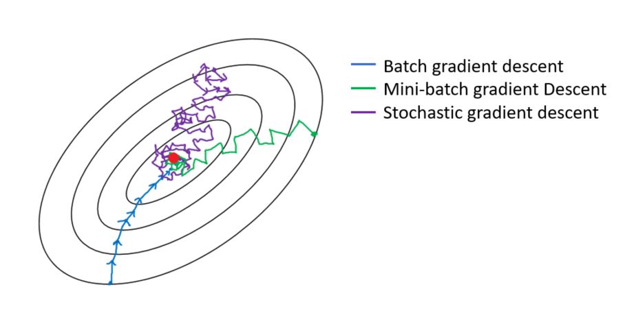
Explain briefly batch gradient descent, stochastic gradient descent, and mini-batch gradient descent? List the pros and cons of each.
- Gradient descent is a generic optimization algorithm capable for finding optimal solutions to a wide range of problems. The general idea of gradient descent is to tweak parameters iteratively in order to minimize a cost function.
- Batch Gradient Descent:
- In Batch Gradient descent the whole training data is used to minimize the loss function by taking a step towards the nearest minimum by calculating the gradient (the direction of descent).
- Pros:
- Since the whole data set is used to calculate the gradient it will be stable and reach the minimum of the cost function without bouncing around the loss function landscape (if the learning rate is chosen correctly).
- Cons:
- Since batch gradient descent uses all the training set to compute the gradient at every step, it will be very slow especially if the size of the training data is large.
- Stochastic Gradient Descent:
- Stochastic Gradient Descent picks up a random instance in the training data set at every step and computes the gradient-based only on that single instance.
- Pros:
- It makes the training much faster as it only works on one instance at a time.
- It become easier to train using large datasets.
- Cons:
- Due to the stochastic (random) nature of this algorithm, this algorithm is much less stable than the batch gradient descent. Instead of gently decreasing until it reaches the minimum, the cost function will bounce up and down, decreasing only on average. Over time it will end up very close to the minimum, but once it gets there it will continue to bounce around, not settling down there. So once the algorithm stops, the final parameters would likely be good but not optimal. For this reason, it is important to use a training schedule to overcome this randomness.
- Mini-batch Gradient:
- At each step instead of computing the gradients on the whole data set as in the Batch Gradient Descent or using one random instance as in the Stochastic Gradient Descent, this algorithm computes the gradients on small random sets of instances called mini-batches.
- Pros:
- The algorithm’s progress space is less erratic than with Stochastic Gradient Descent, especially with large mini-batches.
- You can get a performance boost from hardware optimization of matrix operations, especially when using GPUs.
- Cons:
- It might be difficult to escape from local minima.
- Batch Gradient Descent:
Explain what is information gain and entropy in the context of decision trees?
- Entropy and Information Gain are two key metrics used in determining the relevance of decision making when constructing a decision tree model and to determine the nodes and the best way to split.
- The idea of a decision tree is to divide the data set into smaller data sets based on the descriptive features until we reach a small enough set that contains data points that fall under one label.
- Entropy is the measure of impurity, disorder, or uncertainty in a bunch of examples. Entropy controls how a Decision Tree decides to split the data. Information gain calculates the reduction in entropy or surprise from transforming a dataset in some way. It is commonly used in the construction of decision trees from a training dataset, by evaluating the information gain for each variable, and selecting the variable that maximizes the information gain, which in turn minimizes the entropy and best splits the dataset into groups for effective classification.
What are some applications of RL beyond gaming and self-driving cars?
- Reinforcement learning is NOT just used in gaming and self-driving cars, here are three common use cases you should know in 2022:
-
Multi-arm bandit testing (MAB)
- A little bit about reinforcement learning (RL): you train an agent to interact with the environment and figure out the optimum policy which maximizes the reward (a metric you select).
- MAB is a classic reinforcement learning problem that can be used to help you find a best options out of a lot of treatments in experimentation.
- Unlike A/B tests, MAB tries to maximizes a metric (reward) during the course of the test. It usually has a lot of treatments to select from. The trade-off is that you can draw causal inference through traditional A/B testing, but it’s hard to analyze each treatment through MAB; however, because it’s dynamic, it might be faster to select the best treatment than A/B testing.
-
Recommendation engines
- While traditional matrix factorization works well for recommendation engines, using reinforcement learning can help you maximize metrics like customer engagement and metrics that measure downstream impact.
- For example, social media can use RL to maximize ‘time spent’ or ‘review score’ when recommending content; so this way, instead of just recommending similar content, you might also help customers discover new content or other popular content they like.
-
Portfolio Management
- RL has been used in finance recently as well. Data scientist can train the agent to interact with a trading environment to maximize the return of the portfolio. For example, if the agent selects an allocation of 70% stock, 10% Cash, and 20% bond, the agent gets a positive or negative reward for this allocation. Through iteration, the agent finds out the best allocation.
- Robo-advisers can also use RL to learn investors risk tolerance.
- Of course, self-driving cars, gaming, robotics use RL heavily, but I’ve seen data scientists from industries mentioned above (retail, social media, finance) start to use more RL in their day-to-day work.
You are using a deep neural network for a prediction task. After training your model, you notice that it is strongly overfitting the training set and that the performance on the test isn’t good. What can you do to reduce overfitting?
- To reduce overfitting in a deep neural network changes can be made in three places/stages: The input data to the network, the network architecture, and the training process:
- The input data to the network:
- Check if all the features are available and reliable
- Check if the training sample distribution is the same as the validation and test set distribution. Because if there is a difference in validation set distribution then it is hard for the model to predict as these complex patterns are unknown to the model.
- Check for train / valid data contamination (or leakage)
- The dataset size is enough, if not try data augmentation to increase the data size
- The dataset is balanced
- Network architecture:
- Overfitting could be due to model complexity. Question each component:
- can fully connect layers be replaced with convolutional + pooling layers?
- what is the justification for the number of layers and number of neurons chosen? Given how hard it is to tune these, can a pre-trained model be used?
- Add regularization - ridge (l1), lasso (l2), elastic net (both)
- Add dropouts
- Add batch normalization
- The training process:
- Improvements in validation losses should decide when to stop training. Use callbacks for early stopping when there are no significant changes in the validation loss and restore_best_weights.
Explain the linear regression model and discuss its assumption?
- Linear regression is a supervised statistical model to predict dependent variable quantity based on independent variables.
- Linear regression is a parametric model and the objective of linear regression is that it has to learn coefficients using the training data and predict the target value given only independent values.
- Some of the linear regression assumptions and how to validate them:
- Linear relationship between independent and dependent variables
- Independent residuals and the constant residuals at every \(x\): We can check for 1 and 2 by plotting the residuals(error terms) against the fitted values (upper left graph). Generally, we should look for a lack of patterns and a consistent variance across the horizontal line.
- Normally distributed residuals: We can check for this using a couple of methods: -Q-Q-plot(upper right graph): If data is normally distributed, points should roughly align with the 45-degree line. -Boxplot: it also helps visualize outliers -Shapiro–Wilk test: If the p-value is lower than the chosen threshold, then the null hypothesis (Data is normally distributed) is rejected.
- Low multicollinearity
- You can calculate the VIF (Variable Inflation Factors) using your favorite statistical tool. If the value for each covariate is lower than 10 (some say 5), you’re good to go.
- The figure below summarizes these assumptions.
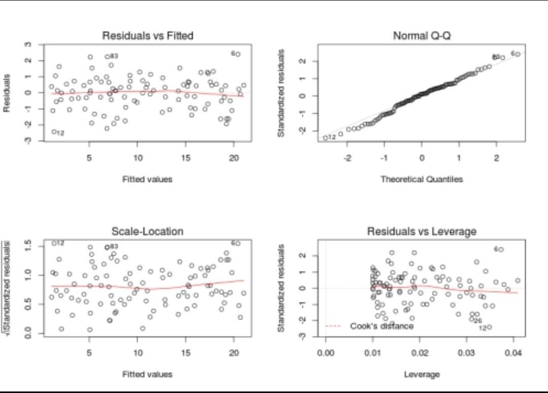
Explain briefly the K-Means clustering and how can we find the best value of K?
- K-Means is a well-known clustering algorithm. K-Means clustering is often used because it is easy to interpret and implement. It starts by partitioning a set of data into \(K\) distinct clusters and then arbitrary selects centroids of each of these clusters. It iteratively updates partitions by first assigning the points to the closet cluster and then updating the centroid and then repeating this process until convergence. The process essentially minimizes the total inter-cluster variation across all clusters.
- The elbow method is a well-known method to find the best value of \(K\) in K-means clustering. The intuition behind this technique is that the first few clusters will explain a lot of the variation in the data, but past a certain point, the amount of information added is diminishing. Looking at the graph below of the explained variation (on the y-axis) versus the number of cluster \(K\) (on the x-axis), there should be a sharp change in the y-axis at some level of \(K\). For example in the graph below the drop-off is at \(k=3\).
- The explained variation is quantified by the within-cluster sum of squared errors. To calculate this error notice, we look for each cluster at the total sum of squared errors using Euclidean distance.
- Another popular alternative method to find the value of \(K\) is to apply the silhouette method, which aims to measure how similar points are in its cluster compared to other clusters. It can be calculated with this equation: \((x-y)/max(x,y)\), where \(x\) is the mean distance to the examples of the nearest cluster, and \(y\) is the mean distance to other examples in the same cluster. The coefficient varies between -1 and 1 for any given point. A value of 1 implies that the point is in the right cluster and the value of -1 implies that it is in the wrong cluster. By plotting the silhouette coefficient on the y-axis versus each \(K\) we can get an idea of the optimal number of clusters. However, it is worthy to note that this method is more computationally expensive than the previous one.
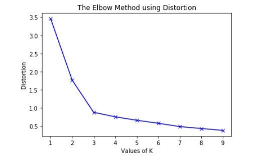
Given an integer array, return the maximum product of any three numbers in the array.
- For example:
A = [1, 5, 3, 4] it should return 60
B = [-2, -4, 5, 3] it should return 40
- If all the numbers are positive, then the solution will be finding the max 3 numbers, if they have negative numbers then it will be the result of multiplying the smallest two negative numbers with the maximum positive number.
- We can use the
heapqlibrary to sort and find the maximum numbers in one step. As shown in the image below.
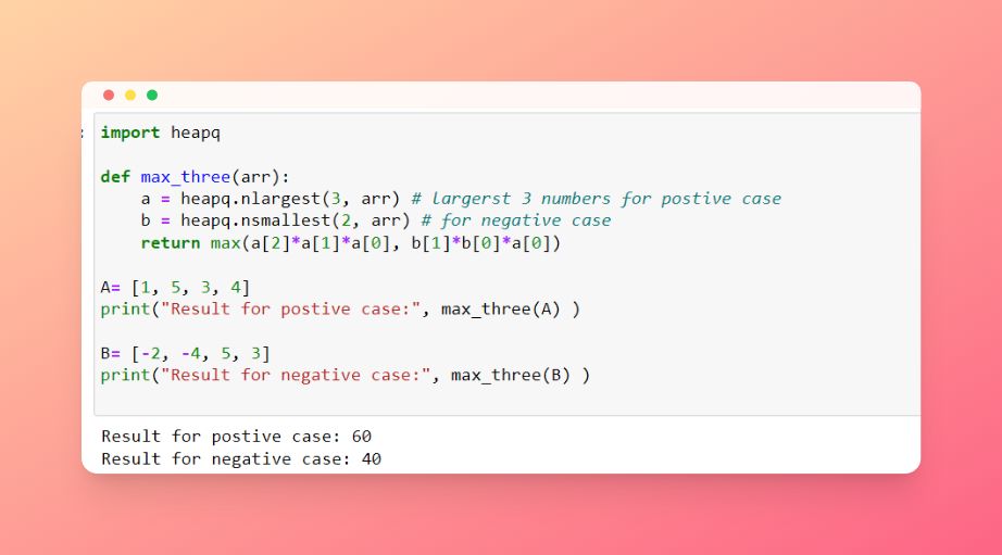
What are joins in SQL and discuss its types?
- A JOIN clause is used to combine rows from two or more tables, based on a related column between them. It is used to merge two tables or retrieve data from there. There are 4 types of joins: inner join left join, right join, and full join.
- Inner join: Inner Join in SQL is the most common type of join. It is used to return all the rows from multiple tables where the join condition is satisfied.
- Left Join: Left Join in SQL is used to return all the rows from the left table but only the matching rows from the right table where the join condition is fulfilled.
- Right Join: Right Join in SQL is used to return all the rows from the right table but only the matching rows from the left table where the join condition is fulfilled.
- Full Join: Full join returns all the records when there is a match in any of the tables. Therefore, it returns all the rows from the left-hand side table and all the rows from the right-hand side table.
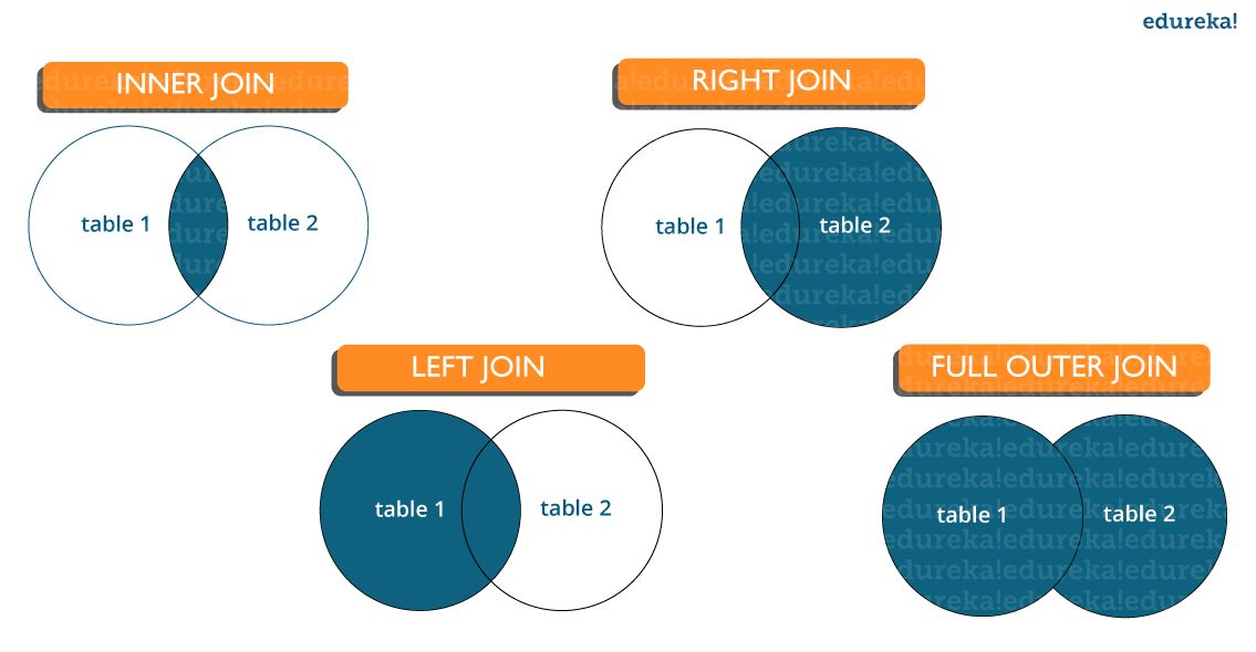
Why should we use Batch Normalization?
- Batch normalization is a technique for training very deep neural networks that standardizes the inputs to a layer for each mini-batch.
- Usually, a dataset is fed into the network in the form of batches where the distribution of the data differs for every batch size. By doing this, there might be chances of vanishing gradient or exploding gradient when it tries to backpropagate. In order to combat these issues, we can use BN (with irreducible error) layer mostly on the inputs to the layer before the activation function in the previous layer and after fully connected layers.
- Batch Normalisation has the following effects on the Neural Network:
- Robust Training of the deeper layers of the network.
- Better covariate-shift proof NN Architecture.
- Has a slight regularization effect.
- Centered and controlled values of Activation.
- Tries to prevent exploding/vanishing gradient.
- Faster training/convergence.
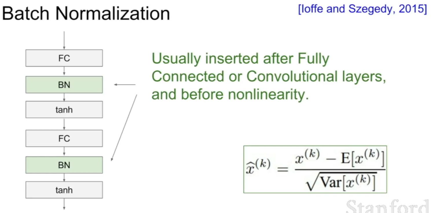
What is weak supervision?
- Weak Supervision (which most people know as the Snorkel algorithm) is an approach designed to help annotate data at scale, and it’s a pretty clever one too.
- Imagine that you have to build a content moderation system that can flag LinkedIn posts that are offensive. Before you can build a model, you’ll first have to get some data. So you’ll scrape posts. A lot of them, because content moderation is particularly data-greedy. Say, you collect 10M of them. That’s when trouble begins: you need to annotate each and every one of them - and you know that’s gonna cost you a lot of time and a lot of money!
- So you want to use autolabeling (basically, you want to apply a pre-trained model) to generate ground truth. The problem is that such a model doesn’t just lie around, as this isn’t your vanilla object detection for autonomous driving use case, and you can’t just use YOLO v5.
- Rather than seek the budget to annotate all that data, you reach out to subject matter experts you know on LinkedIn, and you ask them to give you a list of rules of what constitutes, according to each one of them, an offensive post.
Person 1's rules:
- The post is in all caps
- There is a mention of Politics

Person 2's rules:
- The post is in all caps
- It uses slang
- The topic is not professional

...

Person 20's rules:
- The post is about religion
- The post mentions death
- You then combine all rules into a mega processing engine that functions as a voting system: if a comment is flagged as offensive by at least X% of those 20 rule sets, then you label it as offensive. You apply the same logic to all 10M records and are able to annotate then in minutes, at almost no costs.
- You just used a weakly supervised algorithm to annotate your data.
- You can of course replace people’s inputs by embeddings, or some other automatically generated information, which comes handy in cases when no clear rules can be defined (for example, try coming up with rules to flag a cat in a picture).
What is active learning?
- When you don’t have enough labeled data and it’s expensive and/or time consuming to label new data, active learning is the solution. Active learning is a semi-supervised ML training paradigm which, like all semi-supervised learning techniques, relies on the usage of partially labeled data. Active Learning helps to select unlabeled samples to label that will be most beneficial for the model, when retrained with the new sample.
- Active Learning consists of dynamically selecting the most relevant data by sequentially:
- selecting a sample of the raw (unannotated) dataset (the algorithm used for that selection step is called a querying strategy)
- getting the selected data annotated
- training the model with that sample of annotated training data
- running inference on the remaining (unannotated) data.
- That last step is used to evaluate which records should be then selected for the next iteration (called a loop). However, since there is no ground truth for the data used in the inference step, one cannot simply decide to feed the data where the model failed to make the correct prediction, and has instead to use metadata (such as the confidence level of the prediction) to make that decision.
- The easiest and most common querying strategy used for selecting the next batch of useful data consists of picking the records with the lowest confidence level; this is called the least-confidence querying strategy, which is one of many possible querying strategies. (Technically, those querying strategies are usually brute-force, arbitrary algorithms which can be replaced by actual ML models trained on metadata generated during the training and inference phases for more sophistication).
- Thus, the most important criterion is selecting samples with maximum prediction uncertainty. You can use the model’s prediction confidence to ascertain uncertain samples. Entropy is another way to measure such uncertainty. Another criterion could be diversity of the new sample with respect to exiting training data. You could also select samples close to labeled samples in the training data with poor performance. Another option could be selecting samples from regions of the feature space where better performance is desired. You could combine all the strategies in your active learning decision making process.
- The training is an iterative process. With active learning you select new sample to label, label it and retrain the model. Adding one labeled sample at a time and retraining the model could be expensive. There are techniques to select a batch of samples to label. For deep learning the most popular active learning technique is entropy with is Monte Carlo dropout for prediction probability.
- The process of deciding the samples to label could also be implemented with Multi Arm Bandit. The reward function could be defined in terms of prediction uncertainty, diversity, etc.
- Let’s go deeper and explain why the vanilla form of Active Learning, “uncertainty-based”/”least-confidence” Active Learning, actually perform poorly via real-life datasets:
- Let’s take the example of a binary classification model identifying toxic content in tweets, and let’s say we have 100,000 tweets as our dataset.
- Here is how uncertainty-based AL would work:
- We pick 1,000 (or another number, depending on how we tune the process) records - at that stage, randomly.
- We annotate that data as toxic / not-toxic.
- We train our model with it and get a (not-so-good) model.
- We use the model to infer the remaining 99,000 (unlabeled) records.
- We don’t have ground truth for those 99,000, so we can’t select which records are incorrectly predicted, but we can use metadata, such as the confidence level, as a proxy to detect bad predictions. With least confidence Active Learning, we would pick the 1,000 records predicted with the lowest confidence level as our next batch.
- Go to (2) and repeat the same steps, until we’re happy with the model.
- What we did here, is assume that confidence was a good proxy for usefulness, because it is assumed that low confidence records are the hardest for the model to learn, and hence that the model needs to see them to learn more efficiently.
- Let’s consider a scenario where it is not. Assume now that this training data is not clean, and 5% of the data is actually in Spanish. If the model (and the majority of the data) was meant to be for English, then chances are, the Spanish tweets will be inferred with a low confidence: you will actually pollute the dataset with data that doesn’t belong there. In other words, low confidence can happen for a variety of different reasons. That’s what happens when you do active learning with messy data.
- To resolve this, one solution is to stop using confidence level alone: confidence levels are just one meta-feature to evaluate usefulness.
- In a nutshell, active learning is an incremental semi-supervised learning paradigm where training data is selected incrementally and the model is sequentially retrained (loop after loop), until either the model reaches a specific performance or labeling budget is exhausted.
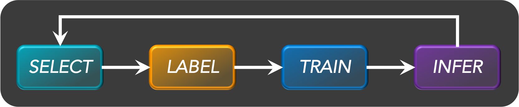
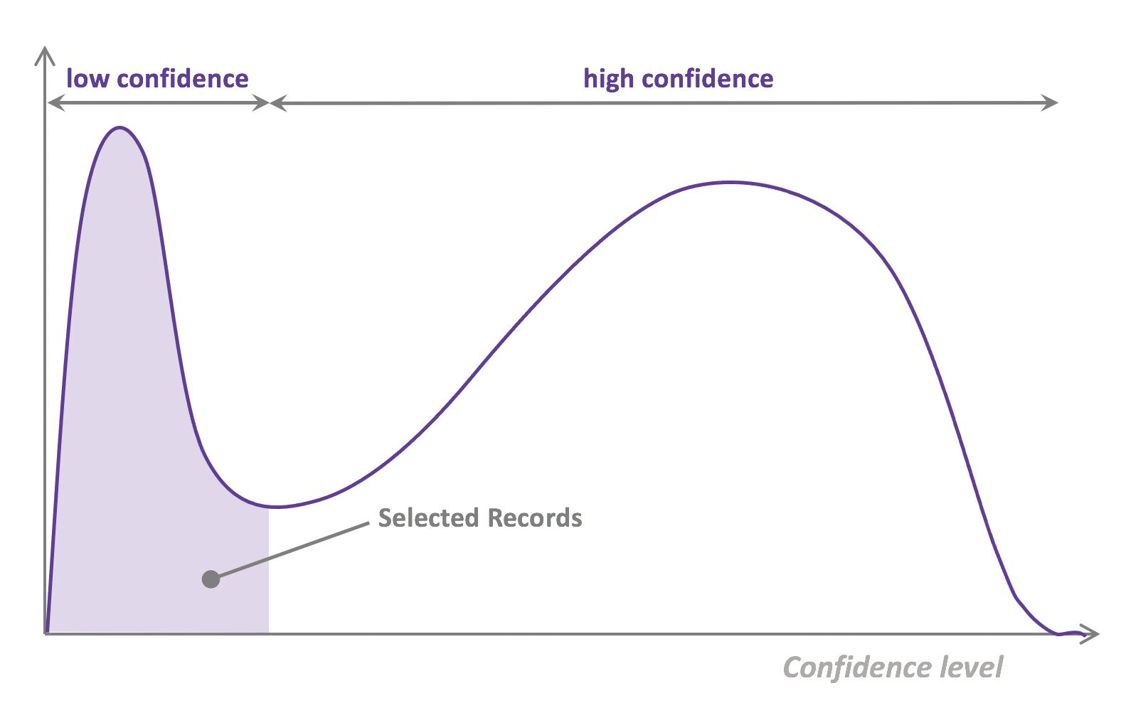
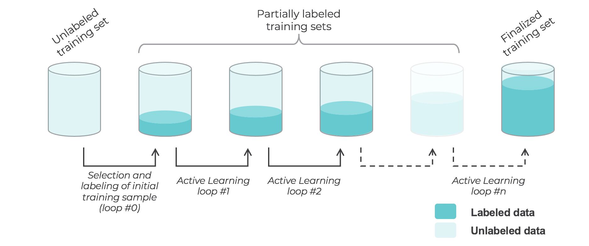
What are the types of active learning?
- There are many different “flavors” of active learning, but did you know that active learning could be broken down into two main categories, “streaming active learning”, and “pooling (batch) active learning”?
- Pooling Active Learning, is when all records available for training data have to be evaluated before a decision can be made about the ones to keep. For example, if your querying strategy is least-confidence, you goal is to select the N records that were predicted with the lowest confidence level in the previous loop, which means all records have to be ranked accordingly to their confidence level. Pooling Active Learning hence requires more compute resources for inference (the entire remainder of the dataset, at each loop, needs to be inferred), but provides a better control of loop sizes and the process as a whole.
- Streaming Active Learning, is when a decision is made “on the fly”, record by record. If your selection strategy was to select all records predicted with a confidence level lower than X% for the previous loop, you’d be doing Streaming AL. This technique obviously requires less compute, and can be used in combination with Online Learning, but it comes with a huge risk: there is no guarantee regarding the amount of data that will be selected. Set the threshold too low, and you won’t select any data for the next loop. Set the threshold too high, and all the remaining data gets selected, and you lose the benefit of AL.
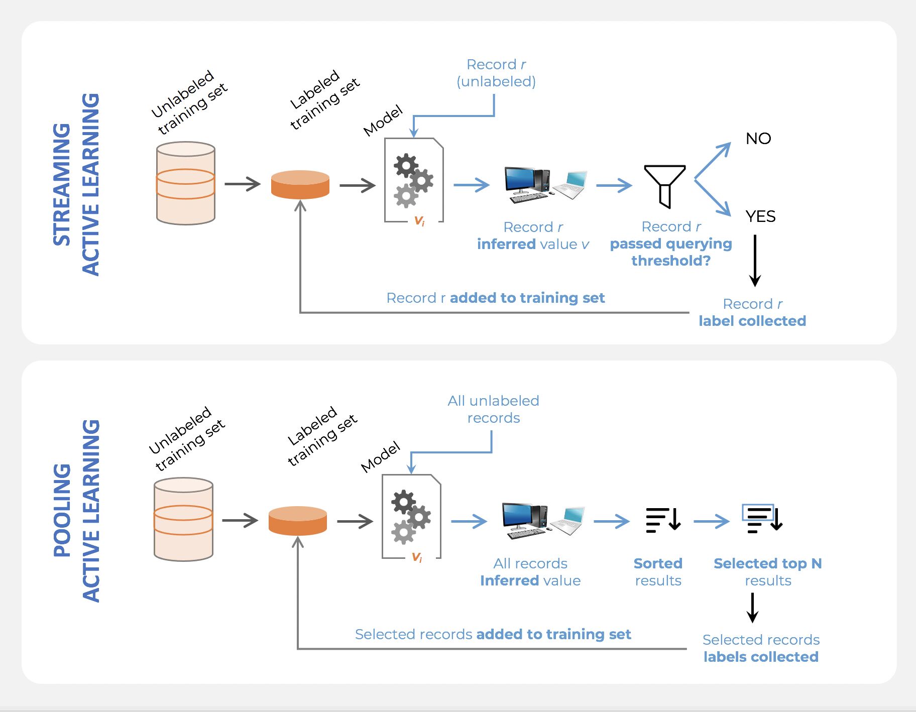
What is the difference between online learning and active learning?
- Online learning is essentially the concept of training a machine learning model on streaming data. In that case, data arrives little-by-little, sequentially, and the model is updated as opposed to be trained entirely from scratch.
- Active learning also consists in training a model sequentially, but the difference is that the training dataset is already fully available. Active learning simply selects small samples of data incrementally; the model is either retrained with the totality of selected records at a given point in time, or updated with the newly selected data.
- Online learning is required when models are to be trained at the point of collection (e.g, on the edge of a device), but active learning, just like supervised learning, usually involves the model being trained offline.
Why is active learning not frequently used with deep learning?
-
Active Learning was relatively popular among ML scientists during the pre-Deep Learning era, and somehow fell out of favor afterwards.
-
The reason why is actually relatively simple: Active Learning usually doesn’t work as well with Deep Learning Models (at least the most common querying strategies don’t). So people gave up on Deep Active Learning pretty quickly. The two most important reasons are the following:
-
The least-confidence, by far the most popular querying strategy, requires the computation of a confidence score. However, the softmax technique which most ML scientists rely on, is relatively unreliable (see this article for details to learn about a better way to compute confidence: https://arxiv.org/pdf/1706.04599.pdf)
-
Active learning, as a process, is actually meant to “grow” a better dataset dynamically. At each loop, more records are selected, which means the same model is retrained with incrementally larger data. However, many hyperparameters in neural nets are very sensitive to the amount of data used. For example, a certain number of epochs might lead to overfitting with early loops and underfitting later on. The proper way of doing Deep Active Learning would be to do hyperparameter tuning dynamically, which is rarely done.
What does active learning have to do with explore-exploit?
- Using the “uncertainty-based”/”least/lowest-confidence” querying strategy as a selection criteria in an active learning process could cause issues when working with a real-life (messy) dataset, as indicated above.
- Uncertainty-based active learning aims at selecting records based on how “certain” (or confident) the model already is about what it knows. Assuming the model can be trusted to self-evaluate properly, then:
- Selecting low confidence records is about picking what the model seems not to know yet; it is a pure exploration process.
- Selecting high confidence records is about picking what the model seems to already know, and that would be about reinforcing that knowledge; it is a pure exploitation process.
- While the “uncertainty-based”/”least/lowest-confidence” querying strategy strategy is the most common using active learning, it might be better to balance exploration and exploitation, and that active learning can and should, in fact, be formulated as a reinforcement learning problem.
What are the differences between a model that minimizes squared error and the one that minimizes the absolute error? and in which cases each error metric would be more appropriate?
- Both mean square error (MSE) and mean absolute error (MAE) measures the distances between vectors and express average model prediction in units of the target variable. Both can range from 0 to infinity, the lower they are the better the model.
- The main difference between them is that in MSE the errors are squared before being averaged while in MAE they are not. This means that a large weight will be given to large errors. MSE is useful when large errors in the model are trying to be avoided. This means that outliers affect MSE more than MAE (because large errors have a greater influence than small errors), that is why MAE is more robust to outliers.
- Computation-wise MSE is easier to use as the gradient calculation will be more straightforward than MAE, since MAE requires linear programming to calculate it.
Define tuples and lists in Python What are the major differences between them?
- Lists:
- In Python, a list is created by placing elements inside square brackets
[], separated by commas. A list can have any number of items and they may be of different types (integer, float, string, etc.). A list can also have another list as an item. This is called a nested list.- Lists are mutable (we can change, add, delete and modify stuff).
- Lists are better for performing operations, such as insertion and deletion.
- Lists consume more memory.
- Lists have several built-in methods.
- In Python, a list is created by placing elements inside square brackets
- Tuples:
- A tuple is a collection of objects which ordered and immutable. Tuples are sequences, just like lists. The differences between tuples and lists are, the tuples cannot be changed unlike lists and tuples use parentheses, whereas lists use square brackets.
- Tuples are immutable (we cannot change, add, delete and modify stuff).
- Tuple data type is appropriate for accessing the elements.
- Tuples consume less memory as compared to the list.
- Tuple does not have many built-in methods.
- A tuple is a collection of objects which ordered and immutable. Tuples are sequences, just like lists. The differences between tuples and lists are, the tuples cannot be changed unlike lists and tuples use parentheses, whereas lists use square brackets.
Given a left-skewed distribution that has a median of 60, what conclusions can we draw about the mean and the mode of the data?
- Left skewed distribution means the tail of the distribution is to the left and the tip is to the right. So the mean which tends to be near outliers (very large or small values) will be shifted towards the left or in other words, towards the tail.
- While the mode (which represents the most repeated value) will be near the tip and the median is the middle element independent of the distribution skewness, therefore it will be smaller than the mode and more than the mean.
- Thus,
- Mean < 60
- Mode > 60
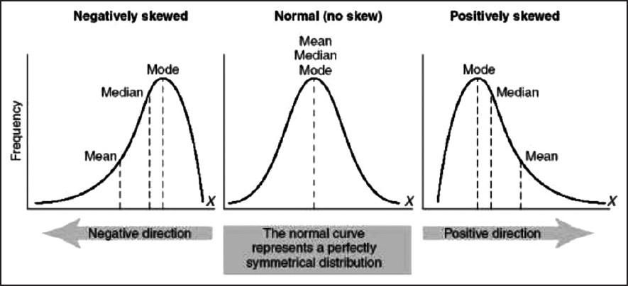
Explain the kernel trick in SVM and why we use it and how to choose what kernel to use?
- Kernels are used in SVM to map the original input data into a particular higher dimensional space where it will be easier to find patterns in the data and train the model with better performance.
- For e.g.: If we have binary class data which form a ring-like pattern (inner and outer rings representing two different class instances) when plotted in 2D space, a linear SVM kernel will not be able to differentiate the two classes well when compared to a RBF (radial basis function) kernel, mapping the data into a particular higher dimensional space where the two classes are clearly separable.
- Typically without the kernel trick, in order to calculate support vectors and support vector classifiers, we need first to transform data points one by one to the higher dimensional space, and do the calculations based on SVM equations in the higher dimensional space, then return the results. The ‘trick’ in the kernel trick is that we design the kernels based on some conditions as mathematical functions that are equivalent to a dot product in the higher dimensional space without even having to transform data points to the higher dimensional space. i.e we can calculate support vectors and support vector classifiers in the same space where the data is provided which saves a lot of time and calculations.
- Having domain knowledge can be very helpful in choosing the optimal kernel for your problem, however in the absence of such knowledge following this default rule can be helpful: For linear problems, we can try linear or logistic kernels and for nonlinear problems, we can use RBF or Gaussian kernels.
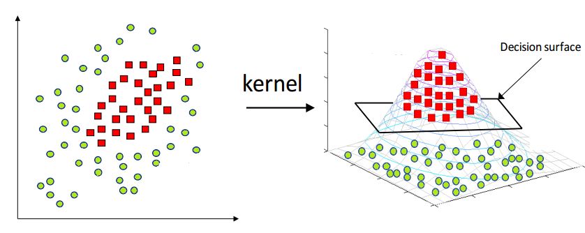
Can you explain the parameter sharing concept in deep learning?
- Parameter sharing is the method of sharing weights by all neurons in a particular feature map. Therefore helps to reduce the number of parameters in the whole system, making it computationally cheap. It basically means that the same parameters will be used to represent different transformations in the system. This basically means the same matrix elements may be updated multiple times during backpropagation from varied gradients. The same set of elements will facilitate transformations at more than one layer instead of those from a single layer as conventional. This is usually done in architectures like Siamese that tend to have parallel trunks trained simultaneously. In that case, using shared weights in a few layers (usually the bottom layers) helps the model converge better. This behavior, as observed, can be attributed to more diverse feature representations learned by the system. Since neurons corresponding to the same features are triggered in varied scenarios. Helps to model to generalize better.
- Note that sometimes the parameter sharing assumption may not make sense. This is especially the case when the input images to a ConvNet have some specific centered structure, where we should expect, for example, that completely different features should be learned on one side of the image than another.
- One practical example is when the input is faces that have been centered in the image. You might expect that different eye-specific or hair-specific features could (and should) be learned in different spatial locations. In that case, it is common to relax the parameter sharing scheme, and instead, simply call the layer a Locally-Connected Layer.
What is the difference between BETWEEN and IN operators in SQL?
BETWEEN–> range between two elements including themselves);IN–> elements in a set(list)- As an simple example:
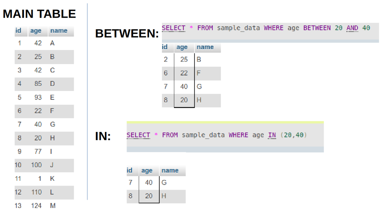
What is the meaning of selection bias and how to avoid it?
-
Sampling bias is the phenomenon that occurs when a research study design fails to collect a representative sample of a target population. This typically occurs because the selection criteria for respondents failed to capture a wide enough sampling frame to represent all viewpoints.
- The cause of sampling bias almost always owes to one of two conditions.
- Poor methodology: In most cases, non-representative samples pop up when researchers set improper parameters for survey research. The most accurate and repeatable sampling method is simple random sampling where a large number of respondents are chosen at random. When researchers stray from random sampling (also called probability sampling), they risk injecting their own selection bias into recruiting respondents.
- Poor execution: Sometimes data researchers craft scientifically sound sampling methods, but their work is undermined when field workers cut corners. By reverting to convenience sampling (where the only people studied are those who are easy to reach) or giving up on reaching non-responders, a field worker can jeopardize the careful methodology set up by data scientists.
- The best way to avoid sampling bias is to stick to probability-based sampling methods. These include simple random sampling, systematic sampling, cluster sampling, and stratified sampling. In these methodologies, respondents are only chosen through processes of random selection—even if they are sometimes sorted into demographic groups along the way.
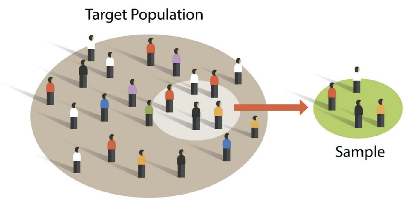
Given two python series, write a function to compute the euclidean distance between them?
- There are different ways to solve this question. The notebook snippet below shows various ways (along with credits to the respetive individual authors) and also shows the computation time for each method. Furthermore, the computation time for each method is calculated depending on whether the input was a NumPy array vs. Python Series and as shown using a NumPy array decreases the computation time.
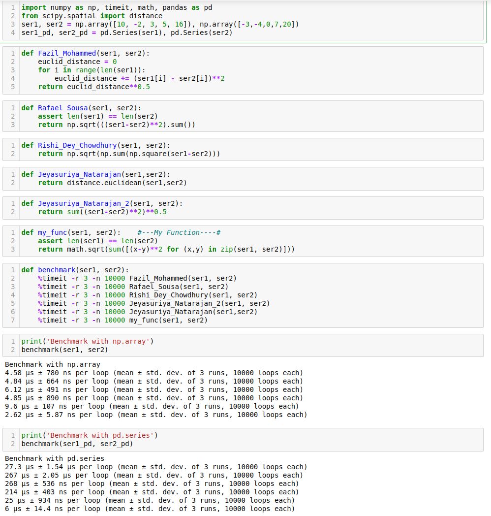
Define the cross-validation process and the motivation behind using it?
-
Cross-validation is a technique used to assess the performance of a learning model in several subsamples of training data. In general, we split the data into train and test sets where we use the training data to train our model and the test data to evaluate the performance of the model on unseen data and validation set for choosing the best hyperparameters. Now, a random split in most cases (for large datasets) is fine. But for smaller datasets, it is susceptible to loss of important information present in the data in which it was not trained. Hence, cross-validation though computationally bit expensive combats this issue.
-
The process of cross-validation is as the following:
- Define \(k\) or the number of folds.
- Randomly shuffle the data into \(k\) equally-sized blocks (folds).
- For each \(i\) in fold (1 to \(k\)), train the data using all the folds except for fold \(i\) and test on the fold \(i\).
- Average the \(k\) validation/test error from the previous step to get an estimate of the error.
- This process aims to accomplish the following:
- Prevent overfitting during training by avoiding training and testing on the same subset of the data points
- Avoid information loss by using a certain subset of the data for validation only. This is important for small datasets.
- Cross-validation is always good to be used for small datasets, and if used for large datasets the computational complexity will increase depending on the number of folds.
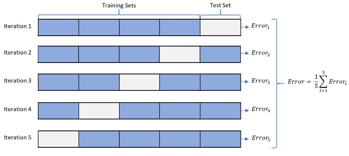
What is the difference between the Bernoulli and Binomial distribution?
- Bernoulli and Binomial are both types of probability distributions.
-
The function of Bernoulli is given by
\[p(x) =p^x * q^(1-x), x=[0,1]\]- where,
- Mean is \(p\).
- Variance \(p*(1-p)\).
- where,
-
The function Binomial is given by:
\[p(x) = nCx p^x q^(n-x) x=[0,1,2...n]\]- where,
- Mean: \(np\).
- Variance: \(npq\). Where p and q are the probability of success and probability of failure respectively, n is the number of independent trials and x is the number of successes.
- where,
- As we can see sample space (\(x\)) for Bernoulli distribution is Binary (2 outcomes), and just a single trial.
- For e.g., a loan sanction for a person can be either a success or a failure, with no other possibility. (Hence single trial).
- Whereas for Binomial the sample space (\(x\)) ranges from \(0-n\).
- As an example, tossing a coin 6 times, what is the probability of getting 2 or a few heads?
- Here sample space is \(x=[0,1,2]\) and more than 1 trial and \(n=6\) (finite).
- In short, Bernoulli Distribution is a single trial version of Binomial Distribution.
Given an integer \(n\) and an integer \(K\), output a list of all of the combinations of \(k\) numbers chosen from 1 to \(n\). For example, if \(n=3\) and \(k=2\), return \([1,2],[1,3],[2,3]\).
- There are different solutions one of them is the one below, there are other solutions in the comments of the original post and also the benchmarking between them thanks to Behnam Hedayat
from itertools import combinations
def find_combintaion(k, n):
	list_num = []
	comb = combinations([k for x in range (1, n+1)], k)
	for i in comb:
		list_num.append(i)

	print("(k: {}, n: {}):".format(k, n))
	print(list_num, "\n")
Explain the long-tailed distribution and provide three examples of relevant phenomena that have long tails. Why are they important in classification and regression problems?
- A long-tailed distribution is a type of heavy-tailed distribution that has a tail (or tails) that drop off gradually and asymptotically.
- Three examples of relevant phenomena that have long tails:
- Frequencies of languages spoken
- Population of cities
- Pageviews of articles
- All of these follow something close to the 80-20 rule: 80% of outcomes (or outputs) result from 20% of all causes (or inputs) for any given event. This 20% forms the long tail in the distribution.
- It’s important to be mindful of long-tailed distributions in classification and regression problems because the least frequently occurring values make up the majority of the population. This can ultimately change the way that you deal with outliers, and it also conflicts with some machine learning techniques with the assumption that the data is normally distributed.
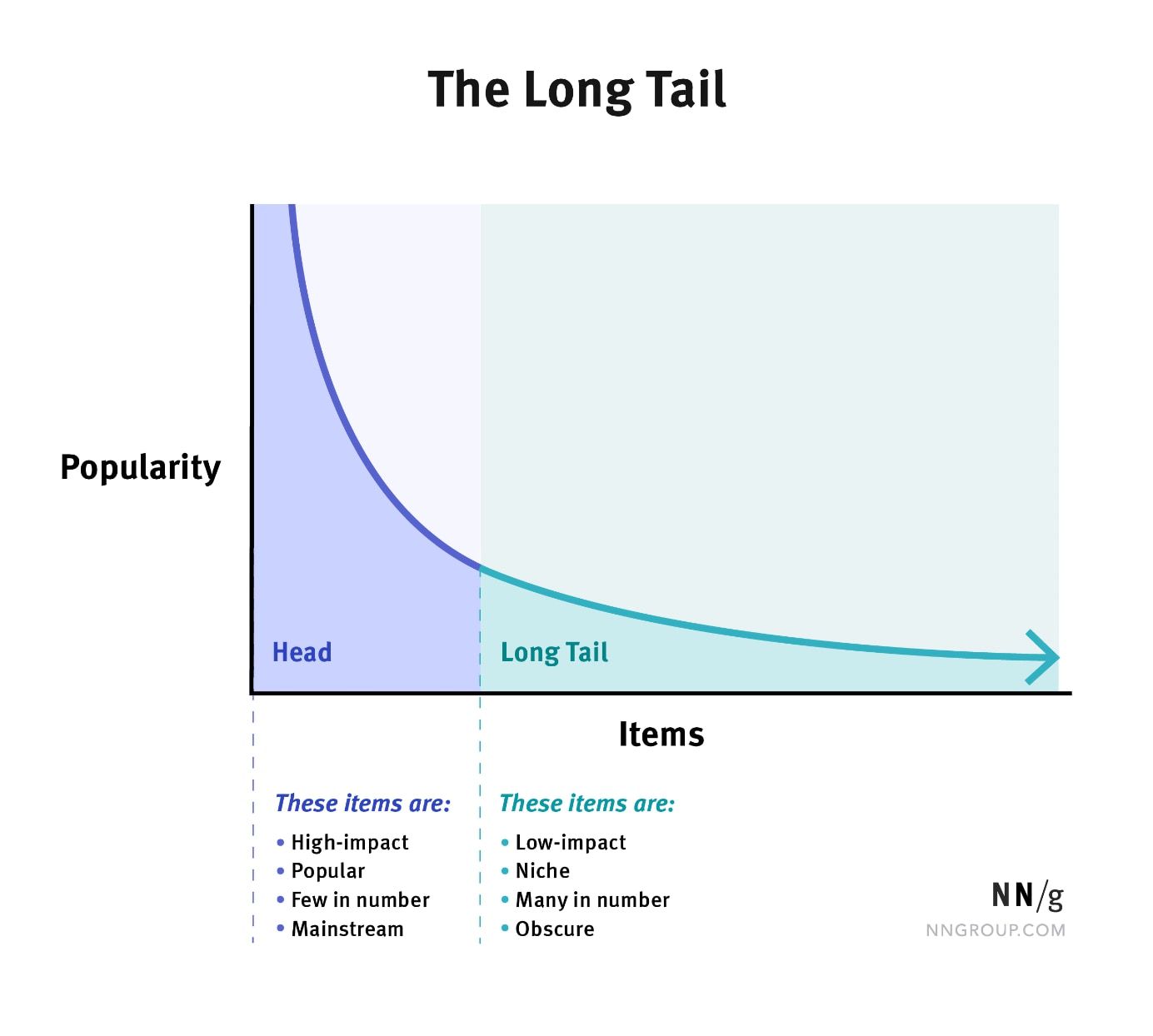
You are building a binary classifier and found that the data is imbalanced, what should you do to handle this situation?
- If there is a data imbalance there are several measures we can take to train a fairer binary classifier:
- Pre-Processing:
- Check whether you can get more data or not.
- Use sampling techniques (Up-sample minority class, downsample majority class, can take the hybrid approach as well). We can also use data augmentation to add more data points for the minority class but with little deviations/changes leading to new data points which are similar to the ones they are derived from. The most common/popular technique is SMOTE (Synthetic Minority Oversampling technique)
- Suppression: Though not recommended, we can drop off some features directly responsible for the imbalance.
- Learning Fair Representation: Projecting the training examples to a subspace or plane minimizes the data imbalance.
- Re-Weighting: We can assign some weights to each training example to reduce the imbalance in the data.
- In-Processing:
- Regularizaion: We can add score terms that measure the data imbalance in the loss function and therefore minimizing the loss function will also minimize the degree of imbalance with respect to the score chosen which also indirectly minimizes other metrics which measure the degree of data imbalance.
- Adversarial Debiasing: Here we use the adversarial notion to train the model where the discriminator tries to detect if there are signs of data imbalance in the predicted data by the generator and hence the generator learns to generate data that is less prone to imbalance.
- Post-Processing:
- Odds-Equalization: Here we try to equalize the odds for the classes w.r.t. the data is imbalanced for correct imbalance in the trained model. Usually, the F1 score is a good choice, if both precision and recall scores are important
- Choose appropriate performance metrics. For example, accuracy is not a correct metric to use when classes are imbalanced. Instead, use precision, recall, F1 score, and ROC curve.
- Pre-Processing:
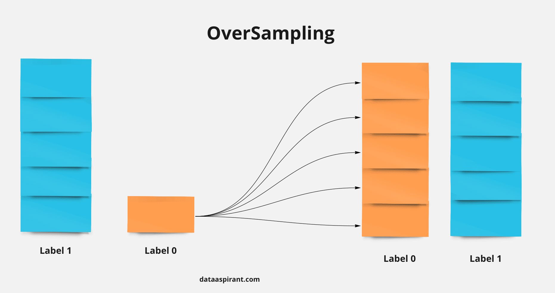
If there are 30 people in a room, what is the probability that everyone has different birthdays?
- The sample space is 365^30 and the number of events is \(365_p_30\) because we need to choose persons without replacement to get everyone to have a unique birthday therefore the Prob = \(365_p_30\) / 365^30 = 0.2936
- Interesting facts provided by Rishi Dey Chowdhury:
- With just 23 people there is over 50% chance of a birthday match and with 57 people the match probability exceeds 99%. One intuition to think of why with such a low number of people the probability of a match is so high. It’s because for a match we require a pair of people and 23 choose 2 is 23*11 = 253 which is a relatively big number and ya 50% sounds like a decent probability of a match for this case.
- Another interesting fact is if the assumption of equal probability of birthday of a person on any day out of 365 is violated and there is a non-equal probability of birthday of a person among days of the year then, it is even more likely to have a birthday match.
- A theoretical explanation is provided in the figure below thanks to Fazil Mohammed.
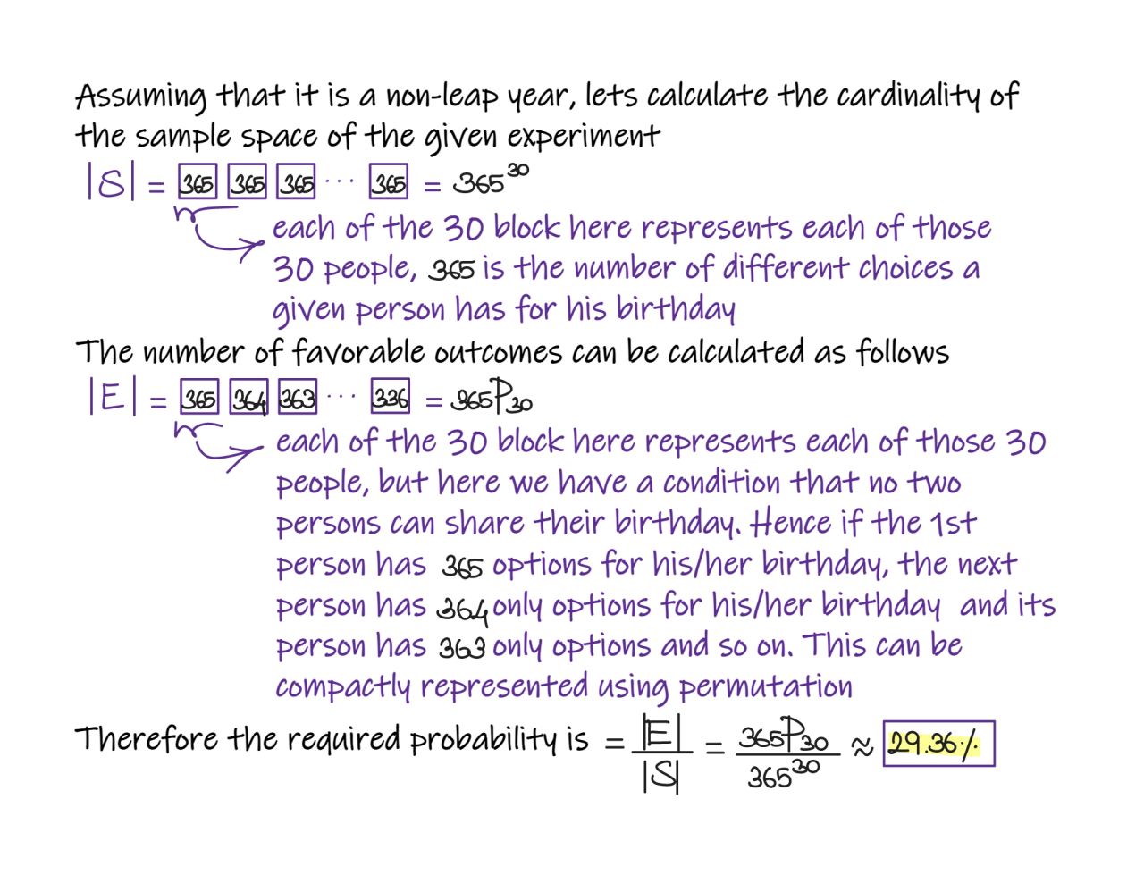
What is the Vanishing Gradient Problem and how do you fix it?
- The vanishing gradient problem is encountered in artificial neural networks with gradient-based learning methods and backpropagation. In these learning methods, each of the weights of the neural network receives an update proportional to the partial derivative of the error function with respect to the current weight in each iteration of training. Sometimes when gradients become vanishingly small, this prevents the weight to change value.
- When the neural network has many hidden layers, the gradients in the earlier layers will become very low as we multiply the derivatives of each layer. As a result, learning in the earlier layers becomes very slow. This can cause the network to stop learning. This problem of vanishing gradients happens when training neural networks with many layers because the gradient diminishes dramatically as it propagates backward through the network.
- Some ways to fix it are:
- Use skip/residual connections.
- Using ReLU or Leaky ReLU over sigmoid and tanh activation functions.
- Use models that help propagate gradients to earlier time steps such as GRUs and LSTMs.
What are Residual Networks? How do they help with vanishing gradients?
- Here is a concept that you should know whether you are trying to get a job in AI or you want to improve your knowledge of AI: residual networks.
- Skip connections or residual networks feed the output of a layer to the input of the subsequent layers, skipping intermediate operations.
- They appear in the Transformer architecture, which is the base of GPT4 and other language models, and in most computer vision networks.
- Residual connections have several advantages:
- They reduce the vanishing gradient since the gradient value is transferred through the network.
- They allow later layers to learn from features generated in the initial layers. Without the skip connection, that initial info would be lost.
- They help to maintain the gradient surface smooth and without too many saddle points.
- This keeps gradient descent to get stuck in local minima, in other words, the optimization process is more robust and then we can use deeper networks.
- ResNet paper was published at the end of 2015 and was very influential because, for the first time, a network with 152 layers surpassed the human performance in image classification.
- Deep learning is based on two competing forces: the more layers, the higher the generalization power of the network, however, the more layers, the more difficult is to optimize.
- In other words, the deeper the network, the better it models the real world in theory, however, it is very difficult to train in practice.
- ResNet was a very important step to solve this problem.
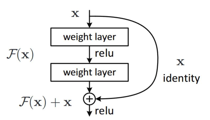
How does ResNet-50 solve the vanishing gradients problem of VGG-16?
- During the ImageNet Large Scale Visual Recognition Challenge (ILSVRC) that with the increase in the number of layers the deep learning models will perform better because of more parameters. However, because of more number of layers, there was a problem with vanishing gradients. In fact, the authors of ResNet, in the original paper, noticed that neural networks without residual connections don’t learn as well as ResNets, although they are using batch normalization, which, in theory, ensures that gradients should not vanish.
- Enter ResNet that utilize skip connections under-the-hood.
- The skip connections allow information to skip layers, so, in the forward pass, information from layer l can directly be fed into layer $l+t$ (i.e., the activations of layer $l$ are added to the activations of layer $l+t$, for $t >= 2$ and, during the forward pass, the gradients can also flow unchanged from layer $l+t$ to layer $l$. This prevents the vanishing gradient problem (VGP). Let’s explain how.
- The VGP occurs when the elements of the gradient (the partial derivatives with respect to the parameters of the network) become exponentially small, so that the update of the parameters with the gradient becomes almost insignificant (i.e., if you add a very small number $0 < \epsilon « 1$ to another number $d$, $d+\epsilon$ is almost the same as d and, consequently, the network learns very slowly or not at all (considering also numerical errors).
- Given that these partial derivatives are computed with the chain rule, this can easily occur, because you keep on multiplying small (finite-precision) numbers.
- The deeper the network, the more likely the VGP can occur. This should be quite intuitive if you are familiar with the chain rule and the back-propagation algorithm (i.e. the chain rule).
- By allowing information to skip layers, layer l+t receives information from both layer $l+t−1$ and layer $l$ (unchanged, i.e., you do not perform multiplications).
- From the paper: “Our results reveal one of the key characteristics that seem to enable the training of very deep networks: Residual networks avoid the vanishing gradient problem by introducing short paths which can carry gradient throughout the extent of very deep networks.”
How do you run a deep learning model efficiently on-device?
- Let’s take the example of LLaMA, a ChatGPT-like LLM by Meta.
- You can run one of the latest LLMs if you have a computer with 4Gb of RAM.
- The model is implemented in C++ (with Python wrappers) and uses several optimization techniques:
- Quantization
- Quantization represents the weights of the model in a low-precision data type like 4-bit integer (INT4) instead of the usual 32-bit floating precision (FP32).
- For example, the smallest LLaMA model has 7B parameters.
- The original model uses 13GB of RAM, while the optimized model uses 3.9GB.
- Faster weight loading
- Another optimization is to load the model weights using
mmap()instead of standard C++ I/O. - That enabled to load LLaMA 100x faster using half as much memory.
mmap()maps the read-only weights usingMAP_SHARED, which is the same technique that’s traditionally used for loading executable software.
- Another optimization is to load the model weights using
- Quantization
When are tress not useful?
- Use tree ensembles (random forest/gradient boosted trees) unless you have a reason not to.
- Here are some of the only reasons not to use tree ensembles for your supervised machine learning problem:
- You are working with unstructured data (text, image, audio, video)
- You are doing statistical inference on a parametric model to draw conclusions (for example, causal inference)
- You have strict interpretability requirements from a legal perspective
- You are trying to model a phenomenon with a known relationship in order to extrapolate the relationship (for example, logistic curves to model population growth scenarios)
- You have very restrictive latency and/or memory requirements (sparse linear models and SVMs are superior here)
- Ignoring these, tree ensembles are typically more adaptable and performant. Spend less time trying to beat them, and more time iterating on data quality, feature engineering, and MLOps best practices.

Gradient descent: Local Minimum vs. Global Minimum
- Gradient descent moves in the direction of the steepest descent of the objective function.
- Without any constraints, the iterative process would lead towards a local minimum by always trying to reduce the objective function value. The critical point here is “local minimum”. Gradient descent, especially in complex functions or when constraints are introduced, doesn’t guarantee finding a global minimum. However, it does guarantee convergence to a local minimum under suitable conditions.
Why can’t the mean squared error be used for classification?
- First, using MSE means that we assume that the underlying data has been generated from a normal distribution (a bell-shaped curve). In Bayesian terms, this means we assume a Gaussian prior. While in reality, a dataset that can be classified into two categories (i.e., binary) is usually not from a normal distribution but a Bernoulli distribution.
- Secondly, the MSE function is non-convex for binary classification.
- As a reminder, a function is non-convex if the function is not a convex function. Non-convex functions are those functions that have many minimum points, in the form of local and global minimum points. The following figure (source) shows the difference between convex and non-convex functions.

- Note that the loss functions that are applied in the context of machine learning models are convex functions, while those applied in the context of neural networks are non-convex functions.
- Put simply, if a binary classification model is trained with the MSE cost function, it is not guaranteed to minimize the cost function. This is because MSE function expects real-valued inputs in range \((-\infty, \infty)\), while binary classification models outputs discrete probabilities in range \((0,1)\) through the sigmoid/logistic function.
- Why Using Mean Squared Error (MSE) Cost Function for Binary Classification is a Bad Idea? offers a great overview of this topic.
What is overfitting? What are some ways to mitigate it?
- Overfitting refers to a modeling error that occurs when a machine learning model is too closely tailored to the specificities of the training data, resulting in poor performance on unseen or new data. Essentially, an overfitted model has learned the training data, including its noise and outliers, so well that it lacks generalization capability to new, unseen data.
- Here’s an analogy: Imagine a student who memorizes specific questions and answers for an exam rather than understanding the underlying concepts. If the exam has the exact questions the student memorized, they will perform well. However, if the exam has different questions that test the same concepts, the student might perform poorly because they only memorized specific answers rather than understanding the topic as a whole.
- Ways to mitigate overfitting include:
- Early stopping: In iterative algorithms, like neural networks, training can be stopped when performance on a validation set starts to degrade, rather than continuing until training error is minimized.
- Regularization: Techniques such as L1 (Lasso) and L2 (Ridge) regularization add a penalty term for complexity to the loss function, discouraging overly complex models. Another regularization technique is dropout, especially used in neural networks, where randomly selected neurons are ignored during training.
- Reduce model complexity: Choose simpler models or reduce the number of parameters in the model. For instance, using a linear regression instead of a high-degree polynomial regression, or using a shallower neural network instead of a very deep one.
- Ensemble methods: Techniques like bagging and boosting, which combine multiple models, can reduce overfitting. For instance, Random Forests use multiple decision trees (an ensemble) and average their predictions, which can help in generalizing better than a single decision tree.
- Gathering more data: If feasible, increasing the amount of training data can help the model generalize better.
- Data augmentation: In areas like image processing, the training data can be augmented by creating new data points through transformations such as rotations, scaling, and cropping. This helps in increasing the effective size of the training dataset.
- Noise injection: Adding a small amount of noise to the training data or even within the model (like in weights of a neural network) can sometimes prevent overfitting, as it encourages the model to learn the underlying patterns rather than the specific noise in the training data.
- Using Bayesian approaches: Bayesian methods, like Bayesian Neural Networks, provide a probabilistic approach to training and can inherently avoid overfitting by considering a distribution over parameters.
- Regularly monitoring and evaluating model performance on a held-out validation set can help in early detection and mitigation of overfitting.
How do you mitigate data imbalance during model training?
- Data imbalance refers to situations where some classes in a classification task have significantly fewer samples than others. This can lead models to favor the majority class (or classes) and perform poorly on the minority class. Here are several methods to mitigate the effects of data imbalance during model training:
- Resampling Techniques:
- Oversampling: Increase the number of instances in the minority class by replicating them or generating synthetic samples.
- Random oversampling: Duplicate random samples from the minority class.
- SMOTE (Synthetic Minority Over-sampling Technique): Create synthetic examples in the feature space.
- ADASYN: Similar to SMOTE but places an emphasis on those instances which are difficult to classify.
- Undersampling: Reduce the number of instances in the majority class. This can lead to a loss of information unless carefully done.
- Random undersampling: Remove random samples from the majority class.
- Tomek links: Remove majority samples that are close to minority samples.
- Cluster centroids: Replace a cluster of majority samples with the cluster centroid.
- NearMiss: Selects majority samples based on their distances to minority class samples.
- Oversampling: Increase the number of instances in the minority class by replicating them or generating synthetic samples.
- Use Different Evaluation Metrics: Accuracy is not a good metric for imbalanced datasets. Instead, consider using:
- Precision, Recall, F1-score
- Area Under the Receiver Operating Characteristic Curve (ROC-AUC)
- Area Under the Precision-Recall Curve (PR-AUC)
- Matthews Correlation Coefficient (MCC)
- Balanced accuracy
- Algorithm-level Approaches:
- Cost-sensitive training: Introduce different misclassification costs for different classes.
- Focal Loss is an alternative to the standard cross-entropy loss for classification, specifically designed to address the issue of class imbalance in deep learning models. It was introduced by Tsung-Yi Lin et al. in the paper “Focal Loss for Dense Object Detection” in the context of object detection, but the principle can be applied to any classification problem.
- The main idea behind focal loss is to reduce the loss contribution from easy-to-classify examples and focus on the hard-to-classify ones. In an imbalanced dataset, the majority of examples are easy-to-classify (i.e., they belong to the majority class), which can overshadow the minority class during training.
- Anomaly (or outlier) detection: Treat the minority class as an anomaly detection problem, by modeling the minority class as a rare event.
- Using tree-based algorithms: Some algorithms like Decision Trees or Random Forests can be less sensitive to data imbalance.
- Cost-sensitive training: Introduce different misclassification costs for different classes.
- Ensemble Methods:
- Bagging with balanced datasets: Bootstrap samples from each class and train ensemble members like Random Forests.
- Boosting: Algorithms like AdaBoost increase the weight of misclassified instances, which can help in focusing on the minority class.
- Balanced Random Forest: Random Forest variant where each tree is grown on a balanced bootstrap sample.
- RUSBoost: A boosting method which combines the principles of boosting with random undersampling.
- Synthetic Data Generation: Use techniques like Variational Autoencoders (VAEs) or Generative Adversarial Networks (GANs) to generate synthetic samples for the minority class.
- Resampling Techniques:
Related: What are some common approaches to improve performance on a long tailed data distribution?
- A long-tail distribution, often observed in real-world datasets, is characterized by a majority of data points belonging to a few “head” categories, while a vast number of categories have very few data points, forming the “tail”. In the context of machine learning, this can lead to challenges, as the model may not perform well on the underrepresented categories in the tail due to the lack of sufficient training examples. Here are some common approaches to improve performance on datasets with long-tail distributions:
- Resampling Techniques:
- Oversampling the tail: This involves creating copies or synthesizing new examples for underrepresented categories. Techniques such as SMOTE or ADASYN can be used for this.
- Undersampling the head: This reduces the number of samples in the overrepresented categories. This approach can be detrimental if done carelessly, as it may throw away potentially useful information.
- Cost-sensitive Learning:
- Assign higher misclassification costs to the tail classes. This way, the algorithm is penalized more for making mistakes on the tail categories, prompting it to pay more attention to them.
- Class Decomposition:
- Decompose multi-class classification into several binary or multi-class tasks, thereby allowing the model to focus on fewer classes at a time.
- Transfer Learning:
- Train a model on a related but balanced dataset and then fine-tune it on the imbalanced, long-tail dataset. The initial training helps the model capture general features, which can aid in recognizing tail classes during fine-tuning.
- Data Augmentation:
- Particularly useful for image data. Augment data in the tail classes by applying transformations such as rotations, translations, zooming, or color jittering to artificially increase the dataset’s size.
- Tail-class Focused Augmentation:
- Apply more aggressive or more frequent augmentations to the tail classes than the head classes, ensuring the model gets a diverse set of examples from the tail classes.
- Hard Example Mining:
- For tasks like object detection, focus on training examples that the model finds challenging, which often belong to the tail classes.
- Meta-learning:
- Techniques like Model-Agnostic Meta-Learning (MAML) can be adapted to long-tail scenarios, enabling the model to learn from few-shot examples, which can be beneficial for tail classes.
- Ensemble Models:
- Combine predictions from several models, potentially giving more weight to models or predictions that focus on tail classes. 10.** Hybrid Models with Memory:**
- Use models that have a memory component, such as Memory Networks or models with a Neural Turing Machine architecture, to remember rare examples from tail classes. 11.** Curriculum Learning:**
- Start training with the head categories and then gradually introduce the tail classes as training progresses. 12.** Binning or Bucketing:**
- Group tail classes into meta-classes or bins and train the model to predict these bins. Once a bin is predicted, a second model can be used to predict the exact class within that bin.
- Resampling Techniques:
- When dealing with long-tail distributions, it’s crucial to measure performance using appropriate metrics. Accuracy might not be informative, as high accuracy can be achieved by merely focusing on the head classes. Metrics like weighted F1-score, macro-average precision, and recall, or area under the precision-recall curve (PR-AUC) may provide a better indication of performance across all classes.
Which ensembling methods work well for class imbalance/long tail scenarios?
- Ensemble methods are strategies that combine multiple models to achieve better performance than any single model alone. For dealing with long-tail distributions, especially in unlabeled data scenarios, certain ensemble techniques can be particularly beneficial:
- Bagging:
- Bootstrap Sampling: This involves taking random subsamples (with replacement) from your dataset to train multiple models. Some of these subsamples might have a higher representation of the tail classes, which can help in capturing their characteristics.
- Random Subspaces: Instead of subsampling data points, random subsets of features are selected for training multiple models. This diversifies the ensemble and can help in capturing nuances of the tail distribution.
- Boosting:
- Boosting algorithms focus on examples that are hard to predict. For long-tail distributions, the tail classes often represent harder examples. Algorithms like AdaBoost or Gradient Boosting can adaptively focus more on these examples in subsequent iterations.
- Stacking:
- Train models with different architectures or algorithms and use their predictions as input features for a meta-model. This can be beneficial since different models might capture different aspects of the tail data.
- Bald Boosting:
- A variant of boosting, where, along with data weights, instance-specific costs are introduced. This allows the algorithm to focus more on tail instances by assigning higher misclassification costs to them.
- Diversity-Aware Ensembles:
- Train multiple models where each model is encouraged to be diverse from others. This can be achieved by using different architectures, different training subsets, different feature subsets, or regularization terms that promote diversity. The goal is to ensure that at least some models in the ensemble are good at capturing the tail data.
- Hierarchical Ensembles:
- Construct ensembles in a hierarchical fashion, where the first level of models might focus on broad patterns (including distinguishing head from tail) and subsequent levels delve deeper into specifics.
- Weighted Ensemble:
- Assign higher weights to models that perform better on tail data when combining their predictions. This gives more importance to models that capture the nuances of the tail distribution.
- Hybrid Ensembles:
- Combine models trained with supervised methods (if some labeled data is available) with models trained on unsupervised methods, thereby leveraging strengths from both supervised and unsupervised paradigms.
- Dynamic Ensemble Selection:
- Rather than combining predictions from all models, dynamically select a subset of models based on the instance to be predicted. Models that are more competent for tail instances can be chosen when predicting such instances.
- Cluster-based Ensembles:
- First, cluster the data, ensuring that tail data is adequately represented in some clusters. Then, for each cluster, train a dedicated model. During prediction, route data points to appropriate models based on their cluster membership or similarity.
- Bagging:
- Remember, when working with long-tail distributions, the evaluation metric is crucial. Ensure that you’re not only looking at overall accuracy but also metrics that can capture performance on the tail classes or instances, such as F1-score, macro-average precision/recall, or other suitable metrics.
What is focal loss? How does it help mitigate class imbalance?
- Focal loss is a modified version of the standard cross-entropy loss used in classification tasks, particularly designed to address class imbalance by focusing more on hard-to-classify examples. It was introduced by Lin et al. in the context of object detection tasks, but it can be applied to any classification problem.
- The formula for focal loss is as follows:
- Binary Classification:
-
For a binary classification task, the focal loss is defined as: \(F L\left(p_t\right)=-\alpha_t\left(1-p_t\right)^\gamma \log \left(p_t\right)\)
-
Where:
- \(p_t\) is the model’s estimated probability for the class with label \(y=1\). Specifically, \(p_t=p\) if \(y=1\) and \(p_t=1-p\) otherwise, with \(p\) being the model’s estimated probability for the class label \(y=1\).
- \(\alpha_t\) is a weighting factor for the class (usually set to address class imbalance), with \(\alpha_t=\alpha\) if \(y=\) 1 and \(\alpha_t=1-\alpha\) otherwise.
- \(\gamma\) is the focusing parameter that smoothly adjusts the rate at which easy examples are downweighted. When \(\gamma=0\), focal loss is equivalent to cross-entropy loss.
-
- Multiclass Classification:
-
For a multiclass classification problem with \(C\) classes, the focal loss can be extended as: \(F L\left(p_t\right)=-\sum_{c=1}^C \alpha_c\left(1-p_{t, c}\right)^\gamma \log \left(p_{t, c}\right)\)
-
Where:
- \(p_{t, c}\) is the predicted probability of the true class \(c\).
- \(\alpha_c\) is the weighting factor for class \(c\).
- \(\gamma\) is the focusing parameter, as in the binary case.
-
- Intuition Behind Focal Loss:
- Handling Class Imbalance: The factor \(\alpha_t\) helps in handling class imbalance by giving more weight to the rare class.
- Focusing on Hard Examples: The term \(\left(1-p_t\right)^\gamma\) reduces the loss contribution from easy examples (where \(p_t\) is large) and increases the contribution from hard examples (where \(p_t\) is small). This focusing parameter \(\gamma\) modulates the effect; the higher the \(\gamma\), the more the model focuses on hard examples.
- Reduction in Dominance of Easy Examples: In imbalanced datasets, the majority class comprises mostly easy examples that can dominate the loss and gradients. Focal loss ensures that the loss is mainly influenced by incorrectly classified examples.
- Focal loss has shown significant improvements in performance for tasks with highly imbalanced datasets, especially in scenarios like object detection, where the background class (negative examples) can significantly outnumber the object classes (positive examples).
- Binary Classification:
How do you define uncertainty with regression problems?
- Uncertainty in regression problems refers to the degree of confidence associated with the model’s predictions. It provides a measure of the model’s “sureness” about its predicted outputs. In the context of regression, uncertainty quantification can be critical for many applications, such as medical or financial predictions, where understanding the reliability of predictions can have significant consequences.
- There are two main types of uncertainties:
- Aleatoric Uncertainty (Data Uncertainty):
- This is inherent variability in the data and cannot be reduced, no matter how much more data you collect.
- It arises due to noise in the observations or inherent variability in the processes being modeled.
- For regression, this can be modeled by predicting a distribution (e.g., Gaussian) for each data point, with the model outputting not just the mean of this distribution but also its variance. 2. Epistemic Uncertainty (Model Uncertainty):
- This uncertainty stems from the model itself. It represents what the model doesn’t know due to lack of data.
- With more data, especially in the underrepresented regions, epistemic uncertainty can be reduced.
- This uncertainty is often captured using techniques like Bayesian neural networks or dropout as a Bayesian approximation.
- Aleatoric Uncertainty (Data Uncertainty):
- To quantify and incorporate uncertainty in regression problems, here are some approaches:
- Prediction Intervals: Generate prediction intervals around the predicted value, which provide a range within which the actual value is likely to fall. Wider intervals indicate greater uncertainty.
- Bayesian Linear Regression: Instead of estimating fixed values for regression coefficients as in standard linear regression, Bayesian linear regression estimates a distribution over possible coefficient values. In other words, Bayesian regression models provide a distribution over the possible values of the regression coefficients, thereby offering a measure of uncertainty.
- Bayesian Neural Networks: Similar to Bayesian Linear Regression, but applied to neural network weights.
- Principle: BNNs model uncertainty by placing a probability distribution over the network’s weights (as opposed to fixed weights in standard neural networks).
- Application: By sampling from these distributions, you can obtain a distribution of predictions for a given input, which reflects the model’s uncertainty.
- Challenge: BNNs can be computationally expensive and complex to implement.
- Monte Carlo (MC) Dropout as a Bayesian Approximation: Using dropout in a neural network not just during training but also during inference can act as an approximation to Bayesian neural networks. Running the model with dropout multiple times for a single input provides a distribution of outputs, capturing the model’s uncertainty.
- Principle: Use dropout not just during training but also during inference. By running multiple forward passes with dropout, you obtain a distribution of predictions.
- Application: The variance in these predictions can be interpreted as a measure of model uncertainty.
- Advantage: Easier to implement than BNNs, as it can be applied to any standard neural network with dropout layers.
- Confidence Calibration:
- Principle: If the model’s confidence scores are not well-calibrated, apply post-hoc calibration methods.
- Techniques: Methods like Platt scaling, isotonic regression, or temperature scaling can adjust the confidence scores to better reflect true probabilities.
- Test-Time Augmentation:
- Principle: Apply various augmentations to the input data at test time.
- Application: Variability in predictions across augmentations can indicate uncertainty.
- Quantile Regression: Instead of predicting a single value, the model is trained to predict quantiles (e.g., 10th percentile, 50th percentile, and 90th percentile). This provides a range of predictions, capturing inherent data uncertainty. In other words, predict different quantiles of the conditional distribution of the response variable, giving an idea of the spread of the possible outcomes.
- Principle: Instead of predicting a single value, predict a range (quantiles) for the output.
- Application: The range between lower and upper quantiles (e.g., 5th and 95th) can represent the prediction uncertainty.
- Gaussian Processes: Gaussian Processes (GPs) are a non-parametric method that provides a probabilistic measure of uncertainty with the predictions. The output of a GP is a distribution over functions, from which you can derive mean predictions and variances.
- Principle: GPs are a Bayesian approach suitable for small to medium-sized datasets.
- Application: They naturally provide a measure of uncertainty (variance) along with predictions.
- Ensemble Methods: Using an ensemble of models (e.g., bagging or bootstrapped ensembles) can provide multiple predictions for each input. The variance or spread of these predictions can be used as a measure of uncertainty. Pu simply, use an ensemble of models and measure the variance in their predictions. A higher variance indicates higher uncertainty.
- Principle: Train multiple models independently and use the variance in their predictions to estimate uncertainty.
- Application: A higher variance in predictions indicates greater uncertainty.
- Types: Bagging, boosting, or stacking different models or the same model with different initializations.
- Likelihood Methods:
- Principle: Model the output distribution of your predictions (e.g., a Gaussian distribution with mean and variance).
- Application: The variance can be used as a measure of uncertainty.
- Adversarial Training:
- Principle: Train the model with adversarial examples.
- Application: This can make the model more robust and its uncertainty estimates more reliable.
- Out-of-Distribution (OOD) Detection
- Principle: Train the model to recognize when inputs are significantly different from the training data.
- Application: OOD inputs often result in higher uncertainty.
- Residual Analysis: Analyze the residuals of the model (the differences between the predicted and actual values). Patterns or high variability in residuals can indicate areas where the model is less certain.
- Homoscedastic & Heteroscedastic Uncertainty: Homoscedastic refers to models where the aleatoric uncertainty is assumed to be constant across all inputs. Heteroscedastic models allow this uncertainty to vary with input data. For regression problems, modeling heteroscedastic uncertainty can be crucial, especially when the noise or variability in the data is input-dependent.
- Addressing Miscalibration:
- Model Calibration Techniques: Implement calibration methods to ensure that the predicted uncertainties align with the actual errors. For example, in probabilistic models, ensuring that the predicted probability distribution matches the observed distribution of the target variable. For miscalibrated models, post-hoc calibration techniques (like Platt scaling or isotonic regression) can be used to adjust the predicted values to better reflect the true likelihoods.
- Improving Model Fit: If the model is miscalibrated, it might be necessary to revisit model selection, feature engineering, or even the data itself to improve the fit.
- Model Calibration Techniques: Implement calibration methods to ensure that the predicted uncertainties align with the actual errors. For example, in probabilistic models, ensuring that the predicted probability distribution matches the observed distribution of the target variable. For miscalibrated models, post-hoc calibration techniques (like Platt scaling or isotonic regression) can be used to adjust the predicted values to better reflect the true likelihoods.
- Choosing the Right Method:
- The choice of method depends on various factors like the size of the dataset, the model complexity, the type of task (regression/classification), and computational resources. In practice, a combination of these methods might be employed to gain a more comprehensive understanding of the model’s uncertainty.
- Understanding and quantifying uncertainty in regression is crucial for making informed decisions based on model predictions, particularly in fields like finance, healthcare, and engineering, where decisions based on model predictions can have significant consequences.
How do we fix distribution shift in machine learning?
- Distribution shift refers to situations where the distribution of the data your model was trained on (source distribution or training distribution) differs from the distribution of the data your model is applied to (target distribution or test distribution). Addressing distribution shift is crucial for ensuring that machine learning models are robust and maintain their performance in real-world scenarios.
- Here are some strategies and techniques to address distribution shift:
- Retraining/Transfer Learning: Regularly retrain your model with recent data or fine-tune on a small labeled subset of the target domain data to adapt to the new distribution.
- Model Ensembles and Stacking: Use an ensemble of models trained on different subsets of the data or under different conditions. This can make the ensemble more robust against distribution shifts.
- Data Augmentation: Expand the training dataset using data augmentation techniques that mimic possible changes in the data distribution.
- Domain Adaptation: This involves adapting a model trained on one domain (source) to work well on a different but related domain (target). Techniques include:
- Feature-level adaptation: Transform source and target feature distributions to be similar using methods like Maximum Mean Discrepancy (MMD) or adversarial training.
- Instance weighting: Assign weights to training instances according to their importance for the target domain.
- Domain-Adversarial Neural Networks: Use a neural network architecture with two objectives: one for the primary task and another adversarial objective that tries to make the feature representations from the source and target domains indistinguishable.
-
Covariate Shift Adaptation: If the shift is due to changes in the input distribution (P(X)), but the conditional distribution P(Y X) remains the same, then re-weighting the training samples to minimize the distribution difference can help. - Concept Drift Detection: Continuously monitor model predictions for signs of declining performance, indicating a possible distribution shift. If detected, the model can be updated.
- Active Learning: Actively query labels for instances in the target domain where the model is uncertain. This can help adapt the model more effectively with fewer labeled examples.
- Neural Architecture Search (NAS): Employ NAS to search for architectures that are robust against distribution shifts.
- Out-of-Distribution (OOD) Detection: Train models to detect OOD samples and handle them separately, either by seeking human intervention or using specialized models.
- Feedback Loops: Implement systems where users can provide feedback on incorrect predictions. This feedback can be used to continuously update and correct the model.
- Anomaly Detection: If the distribution shift leads to anomalous data points, using anomaly detection techniques can help in identifying and handling these anomalies.
- Test-Time Augmentation: Apply various augmentations to each test instance and make predictions on each augmented version. Aggregate these predictions to produce the final prediction.
- Calibration Techniques: Calibrate your model’s predictions to adjust for distribution shifts and ensure that the prediction confidence aligns with the true accuracy.
- When addressing distribution shift, the first step is often to identify and understand its nature. Techniques like visualization, two-sample tests, or measuring divergence metrics can help diagnose the type and magnitude of the shift. Depending on the situation, a combination of the aforementioned strategies might be needed to effectively handle the distribution shift.
What is self-attention?
- Self-attention, a key component of the Transformer architecture, has revolutionized the field of natural language processing due to its effectiveness in modeling complex patterns in sequences. Here’s a breakdown of self-attention:
- Overview:
- Self-attention allows a sequence (e.g., a sentence) to focus on different parts of itself to produce a representation of the sequence. In essence, it lets the model weigh the importance of different words or tokens in relation to a specific word.
- Mechanism:
- Given an input sequence, the self-attention mechanism calculates attention scores for every word against every other word in the sequence. These scores determine how much focus each word in the sequence should have on every other word.
- Query, Key, Value Vectors:
- For each word/token, we derive three vectors:
- Query vector: Represents the word we’re focusing on.
- Key vector: Represents the words we’re comparing against.
- Value vector: Provides the information from each word which we’ll use in our final output.
- These vectors are derived by multiplying the embedding of each word with three weight matrices (which are learned during training).
- For each word/token, we derive three vectors:
- Attention Score Calculation: For a given word’s Query vector, we calculate its dot product with the Key vector of every other word. This gives us the attention scores.
- Softmax: The attention scores are then passed through a softmax function, which converts them to probabilities. This ensures that the scores are normalized and sum up to 1.
- Weighted Sum: The softmax scores for each word are multiplied with their respective Value vectors. The results are summed up to produce the final self-attended representation of the word.
- Multi-Head Attention: Instead of doing this process once, the Transformer architecture does it multiple times in parallel, with each set using different weight matrices. These parallel executions are the “heads” in multi-head attention. The results from each head are concatenated and linearly transformed to produce the final output.
- Advantages of Self-Attention: Long-range Dependencies: Self-attention can capture relationships between words or tokens regardless of their distance in the sequence, unlike RNNs or LSTMs which might struggle with long-range dependencies. Parallelization: Since the attention scores for all word pairs are calculated simultaneously, the process can be parallelized easily, leading to faster training times. Flexibility: The self-attention mechanism is versatile and has been successfully used not just in NLP tasks but also in computer vision and other domains.
- Challenges: Quadratic Complexity: For a sequence of length N, self-attention computes N^2 attention scores. This quadratic complexity can be a bottleneck for very long sequences. Overhead: Despite its parallelizable nature, the sheer number of operations in self-attention can be computationally intensive, especially for tasks that might not need such a complex mechanism.
- The self-attention mechanism, especially within the Transformer architecture, has been the foundation for models like BERT, GPT, T5, and many others that have set state-of-the-art benchmarks in a wide array of NLP tasks.
why do we need Q, K and V in self attention?
- The concepts of Query (Q), Key (K), and Value (V) in self-attention arise from the need to determine the relationship between different elements in a sequence and then utilize this relationship to create a new representation of the sequence. Here’s why each component is essential:
- Query (Q):
- Represents the element we are currently focusing on.
- Allows the model to ask: “Which other elements in the sequence should I attend to, and to what extent, when I’m considering this particular element?”
- In self-attention, every element in the sequence has its own Query representation, as each element seeks to understand its relationship with all other elements.
- Key (K):
- Represents the elements we are comparing against the Query.
- Helps in determining how much attention a Query should pay to each other element.
- The alignment (dot product) of the Query with a Key gives an attention score, indicating the relevance of the corresponding element to the Query.
- Value (V):
- Contains the information that the Query uses once it has identified which parts of the sequence to focus on.
- It’s like the payload that’s being delivered based on the attention scores. The more attention a Query gives to a specific Key, the more of that Key’s Value gets used in the output.
- It helps in updating the representation of the Query based on its relationships with other elements.
- Analogy: Imagine you’re at a party trying to find people you might get along with:
- Query (Q): This is you, wondering whom to talk to next.
- Key (K): These are attributes or vibes from other people at the party. By comparing your interests (Query) with theirs (Key), you determine how much you might get along with each person.
- Value (V): Once you’ve identified someone you’d like to chat with based on the alignment of interests, the conversation (Value) you have with them enriches your experience at the party.
- Why Not Just Use Q and V?
- You might wonder why we can’t just have Queries and Values and skip Keys. The separation of Keys and Values allows for more flexibility and expressiveness in the attention mechanism:
- It decouples the process of determining attention scores (via Q-K alignment) from the content that’s being aggregated (Values).
- This means you can have different transformations for determining attention scores and different transformations for the information you want to aggregate.
- In practice, the distinction between Key and Value transformations enables the attention mechanism to focus on different aspects of the data when determining relationships (Keys) versus when aggregating information (Values).
- In summary, the Q, K, and V setup in self-attention allows the model to determine relationships between elements in a sequence (using Q and K) and then utilize these relationships to compute a new representation of the sequence by aggregating information (using V).
- You might wonder why we can’t just have Queries and Values and skip Keys. The separation of Keys and Values allows for more flexibility and expressiveness in the attention mechanism:
What is the difference between DDPM and DDIM models?
- Denoising Diffusion Probabilistic Models (DDPMs) and Denoising Diffusion Implicit Models (DDIMs) are both types of diffusion models used in deep learning, particularly for generating high-quality, complex data such as images. While they share the same underlying principle of diffusion processes, there are key differences in their approach and characteristics.
- Denoising Diffusion Probabilistic Models (DDPMs):
- Basic Principle: DDPMs work by gradually adding noise to data over a series of steps, transforming the data into a Gaussian noise distribution. The model then learns to reverse this process, generating new data by denoising starting from noise.
- Markov Chain Process: The process involves a forward diffusion phase (adding noise) and a reverse diffusion phase (removing noise). Both phases are modeled as Markov chains.
- Stochastic Sampling: The reverse process in DDPMs is stochastic. This means that during the generation phase, random noise is introduced at each step, leading to variation in the outputs even if the process starts from the same noise.
- Sampling Time: DDPMs typically require a large number of steps to generate a sample, which can be computationally intensive and time-consuming.
- High-Quality Generation: DDPMs have been shown to generate high-quality samples that are often indistinguishable from real data, especially in the context of image generation.
- Denoising Diffusion Implicit Models (DDIMs):
- Modified Sampling Process: DDIMs are a variant of DDPMs that modify the sampling process. They use a deterministic approach instead of a stochastic one.
- Deterministic Sampling: In DDIMs, the reverse process is deterministic, meaning no random noise is added during the generation phase. This leads to consistent outputs for the same starting point.
- Faster Sampling: Because of the deterministic nature and some modifications to the diffusion process, DDIMs can generate samples in fewer steps compared to traditional DDPMs.
- Flexibility in Time Steps: DDIMs offer more flexibility in choosing the number of timesteps, allowing for a trade-off between generation quality and computational efficiency.
- Quality vs. Diversity Trade-off: While DDIMs can generate high-quality images like DDPMs, the lack of stochasticity in the reverse process might lead to less diversity in the generated samples.
- Summary:
- DDPM uses a stochastic process, adding random noise at each step of the reverse process, leading to high diversity in outputs. It requires more steps for sample generation, which makes it slower but excellent at generating high-quality diverse results.
- DDIM employs a deterministic reverse process without introducing randomness in the generation phase. It allows for faster sampling with fewer steps and can generate consistent outputs but might lack the diversity seen in DDPM outputs.
- Both models represent advanced techniques in generative modeling, particularly for applications like image synthesis, where they can generate realistic and varied outputs. The choice between DDPM and DDIM depends on the specific requirements regarding diversity, computational resources, and generation speed.
What is the difference between Tree of Thought prompting and Chain of Thought prompting? Which is better and why?
- “Chain of Thought” prompting and “Tree of Thought” prompting are methods used to enhance the performance of large language models like GPT-3 or GPT-4, particularly on complex tasks that require multi-step reasoning or problem-solving.
- Chain of Thought Prompting
- Principle: In Chain of Thought prompting, the user writes out the intermediate steps or reasoning process that might lead to the answer. This approach helps the model to “think aloud” or follow a logical progression of steps to reach a conclusion.
- Usage: It’s particularly useful for complex problems like math word problems, where simply stating the problem doesn’t provide enough guidance for the model. By including a chain of reasoning, the model is encouraged to follow a similar step-by-step approach.
- Example: For a math problem, the prompt would include both the problem and a sequential, detailed explanation of how to solve it, guiding the model through the reasoning process.
- Tree of Thought Prompting
- Principle: Tree of Thought prompting is a more sophisticated approach where multiple lines of reasoning are considered in parallel. It’s like creating a decision tree where each branch represents a different path of thought or a different aspect of the problem.
- Usage: This method is useful for problems where there might be multiple valid approaches or when the problem’s domain involves dealing with branching possibilities and outcomes.
- Example: In a complex scenario with multiple variables or possible outcomes, the prompt would include an exploration of these different paths, like considering different possible causes for a phenomenon in a scientific problem.
- Comparison and Effectiveness
- Complexity: Tree of Thought is inherently more complex as it involves considering multiple lines of reasoning simultaneously. It’s more comprehensive but also more challenging to structure effectively.
- Applicability: Chain of Thought is generally more straightforward and can be applied to a wide range of problems, especially where a linear, step-by-step approach is beneficial. Tree of Thought is more suited to scenarios with branching possibilities, where multiple factors or outcomes must be considered.
- Efficiency: For simpler problems, Chain of Thought is usually more efficient, as it’s more direct. For more complex, multi-faceted problems, Tree of Thought may provide a more thorough exploration of the problem space.
- Which is Better?: The choice between them depends on the nature of the task. For most straightforward problem-solving tasks, Chain of Thought is sufficient and easier to manage. Tree of Thought is better suited for complex, multi-dimensional problems where different hypotheses or scenarios need to be evaluated.
- In summary, both methods aim to improve the reasoning capabilities of language models by guiding them through a more structured thought process. The choice of which to use should be based on the specific requirements of the problem at hand.
What is mode collapse in GANs?
- Mode collapse is a common issue in the training of Generative Adversarial Networks (GANs). Here’s a breakdown of what it is and why it happens:
- What is Mode Collapse?
- In the context of GANs, “modes” refer to distinct features or patterns in the data distribution. For example, in a dataset of face images, different modes might represent different facial features or expressions.
- Mode collapse occurs when the generator in a GAN starts producing a limited variety of outputs. Instead of capturing the full diversity of the training data (all modes), it focuses on a few modes or even a single mode. This means that the generator keeps producing similar or identical outputs.
- Why Does Mode Collapse Happen?
- GANs consist of two networks: a generator and a discriminator. The generator creates data, and the discriminator evaluates it. The goal of the generator is to produce data indistinguishable from real data, while the discriminator’s goal is to distinguish between real and generated data.
- Mode collapse can occur when the generator finds a particular type of data that consistently fools the discriminator. Instead of continuing to explore and learn the full data distribution, the generator exploits this weakness in the discriminator by producing more of this specific type of data.
- Consequences of Mode Collapse: The primary issue is a lack of diversity in the generated samples, which defeats the purpose of learning the entire distribution of the training data. This limits the utility and effectiveness of the GAN.
What loss functions are generally used in GANs?
- The choice of loss function in GANs can influence their training dynamics and the occurrence of issues like mode collapse. Commonly used loss functions include:
- Minimax (Non-Saturating) Loss: Originally proposed in the seminal GAN paper, it involves a minimax game where the discriminator tries to maximize the loss by correctly classifying real and fake data, while the generator tries to minimize it by fooling the discriminator. A modification of the minimax loss introduces a non-saturating loss term that addresses the issue of vanishing gradients early in training for the generator. It encourages the generator to produce data that the discriminator classifies as real.
- Wasserstein Loss (with Gradient Penalty): Introduced in Wasserstein GANs (WGANs), this loss function measures the Earth Mover’s distance between the real and generated data distributions. It often leads to more stable training and can help mitigate mode collapse. Gradient penalty is sometimes added to enforce a Lipschitz constraint, which further stabilizes training.
- Least Squares GAN Loss: In Least Squares GANs (LSGANs), the loss function is based on the least squares error, which penalizes samples that are far from the decision boundary of the discriminator. This can result in higher quality generated images.
- Hinge Loss: Used in some GAN variants, hinge loss can lead to faster and more stable training.
- Perceptual Loss: Sometimes used in combination with other loss functions, perceptual loss measures high-level perceptual and semantic differences between images, rather than pixel-level differences.
- Each of these loss functions has its strengths and weaknesses, and the choice often depends on the specific application and the nature of the data. Additionally, the design and training procedures of the GAN (e.g., architecture, learning rates, regularization) are also crucial in preventing issues like mode collapse.
What are some transformer-specific regularization methods?
- Transformers have become a cornerstone in modern deep learning, especially for natural language processing tasks. However, their large number of parameters and deep architectures make them prone to overfitting. To mitigate this, several regularization methods specifically suited for Transformers have been developed or adapted:
- Dropout:
- Standard Dropout: Randomly sets a fraction of the input units to 0 at each update during training time, which helps prevent overfitting. In Transformers, dropout is often applied in the fully connected layers, the attention scores, or directly on the embeddings.
- Attention Dropout: Applied specifically to the attention weights, encouraging the model to use a wider range of connections.
- Label Smoothing: This technique involves modifying the target labels to be a mix of the correct label and a uniform distribution over other labels. It prevents the model from becoming too confident about its predictions, which can lead to improved generalization.
- Weight Decay (L2 Regularization): Adding an L2 penalty to the loss function encourages the weights to be small, which can prevent overfitting. This is often implemented as part of the optimizer (e.g., AdamW).
- Layer Normalization: Although primarily used for stabilizing the training process, layer normalization can also have a regularizing effect by controlling the scale of activations.
- Stochastic Depth and Layer Dropout: Randomly dropping entire layers (or residual connections) during training can prevent over-reliance on specific layers and promote redundancy in the network, leading to better generalization.
- Data Augmentation: While not a regularization technique in the traditional sense, data augmentation increases the effective size of the training dataset. For NLP, techniques like back-translation, word or sentence shuffling, or synonym replacement can be used.
- Early Stopping: Monitoring the model’s performance on a validation set and stopping training when performance stops improving can prevent overfitting.
- Gradient Clipping: Capping the gradients during backpropagation to a maximum value can prevent issues with exploding gradients, which can be a form of regularization.
- Temperature Scaling in Softmax: Adjusting the temperature parameter in the softmax function can control the sharpness of the distribution, which can indirectly act as a form of regularization.
- Reducing Model Size: Smaller models with fewer layers or hidden units are less prone to overfitting. Pruning or distillation are methods to reduce model size while trying to retain performance.
- Bayesian Techniques: Implementing Bayesian approaches to model some of the weights or layers in the Transformer. While more computationally intensive, it provides a probabilistic interpretation and can help in regularizing the model.
- Adversarial Training: Introducing small perturbations in the input (adversarial examples) and training the model to be robust against these can improve generalization.
- Sparse Attention Mechanisms: Rather than attending to all tokens in a sequence, sparse attention mechanisms focus on a subset, which can reduce overfitting by preventing the model from relying too heavily on specific parts of the input.
- Dropout:
- Each of these methods has its own merits and can be more or less effective depending on the specific application, the size of the dataset, and the particular architecture of the Transformer model being used. In practice, a combination of several of these techniques is often employed to achieve the best results.
What are transformer specific normalization methods?
-
Transformers, particularly in the context of natural language processing, use specific normalization methods to stabilize and accelerate training. Normalization in deep learning models is crucial for controlling the scale of inputs, weights, or activations, which in turn helps in mitigating issues like vanishing or exploding gradients. For Transformer architectures, the following normalization methods are commonly used:
- Layer Normalization:
- Principle: Unlike batch normalization, which normalizes across the batch dimension, layer normalization performs normalization across the features. For each data point in a mini-batch, it computes the mean and standard deviation used for normalization across all features.
- Application in Transformers: Layer normalization is typically applied just before the self-attention layer and the feed-forward neural network, as well as after the residual connection (i.e., adding the normalized output to the original input of the block).
- Post-Layer Normalization:
- Variation: In some Transformer models, layer normalization is applied after the residual connection (hence post-layer normalization), which has been found to be effective in stabilizing training in some scenarios.
- Impact: This slight modification in the position of the layer normalization can impact training dynamics and model performance.
- Pre-Layer Normalization:
- Alternate Approach: In contrast to post-layer normalization, pre-layer normalization applies the normalization before the residual connection and the self-attention or feed-forward layers. Benefits: This approach has been observed to provide more stable training for Transformers, especially in deeper models or models trained with larger learning rates.
- Scale Normalization:
- Additional Technique: Sometimes used in conjunction with layer normalization, scale normalization involves scaling down the weights of the self-attention layers. This can help in managing the magnitude of the outputs in these layers, contributing to more stable training.
- Batch Normalization:
- Less Common in Transformers: While batch normalization is widely used in CNNs, it’s less common in Transformers due to the dynamic nature of sequence lengths and the batch-wise computation it requires. However, it has been explored in some Transformer variants.
- Weight Normalization:
- Alternative Approach: Weight normalization is another technique that decouples the length of the weight vector from its direction. It’s not as commonly used in standard Transformer models but can be considered in custom architectures.
- RMSNorm:
- Variant of Layer Norm: RMSNorm is a simplified version of layer normalization that normalizes the activations by their root mean square (RMS). It omits the bias and gain parameters of layer normalization, potentially simplifying the training process.
- Power Normalization:
- Emerging Approach: Power normalization is an alternative to layer normalization that stabilizes the second-order moments of the activations. It’s a relatively new approach and is being explored in the context of Transformer models.
- The choice of normalization method can significantly affect the training efficiency and final performance of Transformer models. Layer normalization and its variants (pre and post) are currently the most widely used due to their effectiveness in handling variable sequence lengths and their compatibility with the Transformer architecture’s requirements.
What is curriculum training? What does it do to the loss surface?
- Curriculum learning is a training strategy in machine learning inspired by the way humans learn progressively, starting from simpler concepts and gradually moving to more complex ones. This concept was introduced by Bengio et al. and is based on the idea that starting training with easier examples and gradually increasing the difficulty can improve both the speed and effectiveness of the learning process.
- How Curriculum Training Works
- Sorting Training Examples: Initially, you sort or group the training examples based on their difficulty. What constitutes “difficulty” can vary depending on the task (e.g., the length of sentences in language tasks, the clarity of images in vision tasks).
- Gradual Complexity Increase: Training begins with the simplest examples. As the model’s performance improves, more complex examples are gradually introduced into the training process.
- Dynamic Adjustment: The pace at which complexity is increased can be dynamic, based on the model’s current performance and learning rate.
- Impact on the Loss Surface
- Curriculum learning can have several impacts on the loss surface and the optimization process:
- Smoothing the Loss Landscape: Starting with simpler examples can smooth out the loss landscape initially, making it easier for the optimization algorithm (like gradient descent) to find a good path towards the minima.
- Avoiding Local Minima: By simplifying the early stages of training, the model may avoid getting stuck in local minima that are more common in complex, high-dimensional loss surfaces.
- Better Generalization: There is evidence suggesting that curriculum learning can lead to solutions that generalize better to unseen data. This could be because the model first learns broad, general patterns before fine-tuning on more complex and specific features.
- Faster Convergence: It can accelerate the training process, as the model initially works with less complex data, allowing for quicker improvements in performance.
- Guided Feature Learning: In the context of deep learning, starting with simpler tasks can guide the model to learn foundational features first, which can be built upon with more complex features as training progresses.
- Applications and Variations
- Curriculum Learning in NLP: For language models, curriculum learning might involve starting with shorter or simpler sentences before introducing longer or more complex syntax.
- In Computer Vision: Begin with clearer, easier-to-classify images, and then gradually introduce images with more noise or ambiguity.
- Self-Paced Learning: A variant where the model itself helps to determine the sequence of training examples based on its current performance.
- Task-Level Curriculum: Involves starting with easier tasks and gradually moving to harder tasks, which is particularly relevant in multi-task learning scenarios.
- In summary, curriculum learning reshapes the training process to make it more efficient and effective, potentially leading to smoother optimization paths and better generalization. However, designing an effective curriculum requires domain knowledge and understanding of what constitutes “easy” and “difficult” examples in the context of the specific problem being addressed.
What are types of ensemble models? Why do they perform better than regular models?
- Ensemble models in machine learning combine multiple learning algorithms to obtain better predictive performance than could be obtained from any of the individual learning algorithms alone. The key idea behind ensemble methods is that by averaging out biases, reducing variance, and improving predictions, the ensemble’s performance is typically stronger than that of a single model. There are several types of ensemble models:
- Bagging (Bootstrap Aggregating)
- Mechanism: It involves training multiple models in parallel, each on a random subset of the data (with replacement), and then averaging their predictions.
- Example: Random Forest is a classic example of a bagging ensemble, where multiple decision trees are trained on different subsets of the dataset.
- Advantage: Bagging reduces variance and helps to avoid overfitting.
- Boosting
- Mechanism: In boosting, models are trained sequentially, with each model learning from the errors of the previous ones. The predictions are then combined, typically through a weighted sum.
- Examples: XGBoost, AdaBoost, and Gradient Boosting are popular boosting algorithms.
- Advantage: Boosting focuses on reducing bias (and also variance), which can lead to very accurate models, especially on structured data like tables.
- Stacking (Stacked Generalization)
- Mechanism: Different models are trained independently, and a new model, often referred to as a meta-model or blender, is trained to combine these individual predictions**.
- Example: The base level might consist of various algorithms like decision trees, neural networks, and SVMs, and the meta-model could be a logistic regression.
- Advantage: Stacking captures different aspects of the data through diverse models and combines them for improved accuracy.
- Voting
- Mechanism: In a voting ensemble, multiple models are trained independently, and their predictions are combined through majority voting (for classification) or averaging (for regression).
- Types: Hard voting (based on predicted labels) and soft voting (based on predicted probabilities).
- Advantage: Voting ensembles are simple to implement and can lead to improved performance, especially when combining models with very different methodologies.
- Bagging (Bootstrap Aggregating)
- Why Do Ensemble Models Perform Better?
- Reduction in Variance: By averaging multiple predictions, the ensemble’s variance is reduced. This is especially true in bagging, where the individual models may overfit the data.
- Reduction in Bias: In boosting, models sequentially focus on the hard-to-predict instances, thereby reducing bias.
- Exploiting Strengths of Individual Models: Different models have different strengths and weaknesses. Ensembles can combine these models in a way that amplifies their strengths while compensating for their weaknesses.
- Diversity of Perspectives: Multiple models provide a variety of “opinions” on the data, capturing different patterns and relationships that a single model might miss.
- Improved Predictive Performance: The combination of lower variance, lower bias, and capturing a richer set of patterns generally leads to better overall predictive performance compared to individual models.
- Robustness: Ensemble models are typically more robust to outliers and less likely to be thrown off by peculiarities of a single dataset.
- Considerations: While ensemble methods often outperform single models, they are not without drawbacks. They can be more computationally expensive, harder to interpret, and require more resources to train and deploy. Therefore, the decision to use an ensemble approach should consider these trade-offs against the potential benefits in improved performance.
Why should you make inductive biases in models? What can’t we consider the whole search space?
- Inductive biases in machine learning models refer to the set of assumptions the model makes about the underlying pattern it’s trying to learn from the data. These biases guide the learning algorithm to prefer certain solutions over others. Implementing inductive biases is essential for several reasons, and there are practical limitations to considering the entire search space in machine learning tasks.
- Why Inductive Biases are Necessary:
- Feasibility of Learning: Without any inductive biases, a learning algorithm would not be able to generalize beyond the training data because it would have no preference for simpler or more probable solutions over more complex ones. In the absence of inductive biases, the model could fit the training data perfectly but fail to generalize to new, unseen data (overfitting).
- Curse of Dimensionality: As the dimensionality of the input space increases, the amount of data needed to ensure that all possible combinations of features are well-represented grows exponentially. Inductive biases help to reduce the effective dimensionality or the search space, making learning feasible with a realistic amount of data.
- No Free Lunch Theorem: This theorem states that no single learning algorithm is universally better than others when averaged over all possible problems. Inductive biases allow algorithms to specialize, performing better on a certain type of problem at the expense of others.
- Computational Efficiency: Exploring the entire hypothesis space is often computationally infeasible, especially for complex problems. Biases help reduce the search space, making training more computationally efficient.
- Incorporating Domain Knowledge: Inductive biases can be a way to inject expert knowledge into the model, allowing it to learn more efficiently and effectively. For example, convolutional neural networks are biased towards image data due to their architectural design, which is suited for spatial hierarchies in images.
- Limitations of Exploring the Whole Search Space:
- Computational Constraints: The size of the complete hypothesis space for even moderately complex models can be astronomically large, making it computationally impossible to explore thoroughly.
- Risk of Overfitting: Without biases, models are more likely to fit noise in the training data, leading to poor generalization.
- Data Limitations: In practice, we have limited data. Without biases guiding the learning process, the amount of data required to learn meaningful patterns would be impractically large.
- Interpretability and Simplicity: Models learned without biases tend to be more complex and harder to interpret. Simpler models (encouraged by appropriate biases) are often preferred because they are easier to understand, debug, and validate.
- Conclusion:
- In summary, inductive biases in machine learning models are crucial for guiding the learning process, making it computationally feasible, and ensuring that models generalize well to new, unseen data. These biases are a response to practical limitations in data availability, computational resources, and the inherent complexity of learning tasks.
How do you identify if a model is hallucinating? What are some mitigation strategies?
-
Identifying if a machine learning model, especially a language model like GPT-3 or GPT-4, is “hallucinating” — that is, generating false or nonsensical information — can be a crucial aspect of evaluating its reliability and suitability for various applications. Hallucinations in this context refer to the model confidently generating outputs that are incorrect, irrelevant, or nonsensical.
- Strategies to Identify Model Hallucination:
- Result Verification: Cross-reference the model’s outputs with trusted sources or ground truth data. This is especially important for factual information where accuracy is critical. This can be done in an automated manner (looking up factual information on the web and performing NLI on the model’s output vs. web information) or with a human-in-the-loop setup. In many cases, especially for complex tasks like story generation or open-ended question answering, human judgment is crucial to evaluate the sensibility and correctness of the output.
- Consistency Checks: Test the model with similar or paraphrased queries to see if it provides consistent answers. Inconsistent responses can indicate hallucinations.
- Sensitivity Analysis: Analyze how slight changes in the input affect the output. Excessive sensitivity or dramatic changes in output for minor input modifications can suggest hallucinatory behavior.
- Out-of-Distribution Detection: Check how the model performs on data that is significantly different from the training data. Poor handling of such data might lead to hallucinations.
- Error Analysis: Perform a detailed analysis of the model’s errors. Categorize these errors to understand if they are due to hallucinations or other issues like overfitting or underfitting.
- Challenge with Counterfactuals: Present the model with counterfactual or hypothetical scenarios. Models prone to hallucination may struggle to handle such inputs appropriately.
- Model Confidence Assessment: For models that output confidence scores (like some classification models), compare these scores with actual performance. Overconfidence in incorrect answers can be a sign of hallucination.
- Benchmarking Against Known Tasks: Compare the model’s performance on well-established datasets or tasks where the expected outputs are known.
- Input Truncation Tests: Truncate or alter inputs to see if the model still generates plausible outputs. Illogical outputs in response to incomplete or nonsensical inputs can indicate a tendency to hallucinate.
- Preventing or Mitigating Hallucinations:
- Training Data Quality and Diversity: Ensure the training data is diverse, high-quality, and representative of the problem space.
- Regularization and Fine-tuning: Apply techniques to prevent overfitting and fine-tune the model on specific domains or types of data to improve its accuracy.
- Explicitly Modeling Uncertainty: In some cases, incorporating mechanisms for the model to express uncertainty can be helpful.
- Post-Processing Rules: Implement rules or filters to catch and correct certain types of hallucinations.
- User Feedback Loop: Incorporate user feedback to continuously improve the model and reduce hallucinations over time.
- Identifying hallucinations in AI models is particularly important in scenarios where trust, safety, and accuracy are critical, such as in medical, financial, or legal applications. Regular monitoring and evaluation are essential to ensure that the models perform reliably and sensibly in their intended applications.
Why were RNNs introduced? How are LSTMs different and what issue do they solve?
- Recurrent Neural Networks (RNNs) were introduced to handle sequential data, where the order and context of data points are important. Before RNNs, traditional neural networks, like feed-forward networks, assumed that all inputs (and outputs) were independent of each other, which limited their ability to model data where the sequence matters, like time series or text.
- Why RNNs Were Introduced:
- Handling Sequences:**: RNNs are designed to process sequences of data by maintaining a ‘memory’ (hidden state) of previous inputs. This allows them to capture information about the sequence as a whole.
- Variable-Length Inputs:: They can handle inputs of varying lengths, unlike traditional neural networks that require fixed-sized inputs.
- Parameter Sharing Across Time:: RNNs use the same weights while processing different time steps of the sequence, making them more efficient and reducing the number of parameters.
- Applications in Time Series and NLP:: They became a natural choice for time series analysis, natural language processing, speech recognition, and other tasks involving sequential data.
- Limitations of RNNs and Introduction of LSTMs: However, standard RNNs have significant limitations:
- Vanishing Gradient Problem:: During backpropagation, RNNs suffer from the vanishing (and sometimes exploding) gradients problem, making it difficult to learn long-range dependencies in sequences.
- Limited Memory:: They can struggle with retaining information from early time steps in long sequences.
- Lack of a mechanism to add or remove information: Traditional Recurrent Neural Networks (RNNs) do not have gates in the same sense as Long Short-Term Memory (LSTM) units or Gated Recurrent Units (GRUs). The basic architecture of a traditional RNN is simpler and does not include the sophisticated gating mechanisms that are characteristic of LSTMs and GRUs.
- How LSTMs Solve These Issues: Long Short-Term Memory networks (LSTMs), a type of RNN, were introduced to overcome these limitations.
- Memory Cells:: LSTMs have a complex mechanism with memory cells that can store information for long periods. The key components of these cells are the input, output, and forget gates.
- Gates Mechanism::
- Input Gate: Controls how much of the new information should be added to the cell state.
- Forget Gate: Decides what information should be discarded from the cell state.
- Output Gate: Controls the output of the cell state to the next hidden state.
- Long-Range Dependencies: The gated structure of LSTMs allows them to learn which data in the sequence is important to keep or throw away, thus mitigating the vanishing gradient problem and enabling them to capture long-range dependencies.
- Better Memory Management:: The ability to add or remove information from the cell state selectively allows LSTMs to maintain longer-term dependencies.
- Summary: In summary, RNNs were introduced to model sequential data, a task that traditional neural networks weren’t equipped for. LSTMs evolved as a special kind of RNN to address the vanishing gradient problem and to better capture long-range dependencies within the input sequences. This made LSTMs particularly effective for complex sequential tasks like language modeling, machine translation, and speech recognition.
What is the need for DL models? Explain traditional ML models and cases where they would fail?
-
Deep Learning (DL) models and traditional Machine Learning (ML) models serve different purposes and excel in various types of tasks. Understanding their strengths and limitations is crucial in selecting the right approach for a given problem.
- Traditional Machine Learning Models: Traditional ML models include algorithms like linear regression, logistic regression, decision trees, random forests, support vector machines (SVMs), and k-nearest neighbors (k-NN). These models are often preferred for their simplicity, interpretability, and efficiency on smaller or structured datasets.
- Strengths:
- Efficiency: They generally require less computational resources.
- Interpretability: Many traditional models are easier to interpret and understand, which is crucial in domains like finance and healthcare.
- Small Data: They can perform well with smaller datasets.
- Limitations:
- Feature Engineering: Traditional ML models often rely heavily on feature engineering, i.e., manually creating and selecting the most relevant features from the data.
- Handling High-Dimensional Data: They might struggle with very high-dimensional data or data with complex structures, like images and natural language.
- Modeling Complex Patterns: Traditional models can be limited in their ability to capture complex, non-linear relationships in data.
- Strengths:
- Deep Learning Models: Deep Learning models, particularly neural networks, are designed to learn hierarchical representations of data, making them extremely effective for tasks involving unstructured data like images, audio, and text.
- Strengths:
- Handling Unstructured Data: DL models excel in tasks involving high-dimensional and unstructured data (e.g., image and speech recognition, natural language processing).
- Automatic Feature Extraction: They automatically learn and extract features from raw data, reducing the need for manual feature engineering.
- Modeling Complex Patterns: Deep neural networks are capable of modeling highly complex and non-linear relationships.
- Limitations:
- Data Requirements: DL models usually require large amounts of labeled training data.
- Computational Resources: They are computationally intensive and require more processing power, often necessitating GPUs for training.
- Interpretability: Deep Learning models are often considered “black boxes” due to their complexity, making them less interpretable.
- Strengths:
- Cases Where Traditional ML Models Might Fail:
- Image Recognition: Tasks like object detection or facial recognition involve processing high-dimensional pixel data and recognizing complex patterns, something traditional ML models are generally not equipped to handle effectively.
- Natural Language Processing: Tasks like machine translation, sentiment analysis, or question-answering involve understanding human language’s nuances, context, and syntax. Traditional ML struggles with such tasks due to the complexity and variability of language.
- Sequence Data: Handling sequence data (like time-series forecasting with long sequences or predicting the next word in a sentence) can be challenging for traditional ML models. Deep Learning models, especially RNNs, LSTMs, and Transformers, are more adept at capturing long-range dependencies in sequences.
- In summary, the choice between traditional ML and DL models depends on the nature of the task, the type and amount of data available, the need for interpretability, and the computational resources at hand. While traditional models are effective for structured data and provide simplicity and interpretability, DL models are better suited for tasks involving complex patterns and high-dimensional, unstructured data.
In self-attention, why do we use projections of K,Q,V instead of the original values?
- In self-attention mechanisms, particularly those used in Transformer models, the use of projections (linear transformations) for Key (K), Query (Q), and Value (V) vectors, instead of their original values, is a crucial design choice that offers several benefits:
- Increasing Model Capacity and Flexibility:
- Learning Task-Specific Representations: By projecting the inputs into Q, K, and V spaces, the model can learn representations that are specifically tailored for the task of attention. This is analogous to feature learning, where the model learns the most effective ways to represent data for a specific task.
- Dimensionality Control: Projections allow control over the dimensionality of the Q, K, and V vectors. This is important for computational efficiency and to ensure that the dot-products (used in calculating attention scores) don’t grow too large with increasing input size.
- Model Depth and Complexity: Using different projections for each head in multi-head attention allows the model to capture different types of relationships. Each head can focus on different parts of the input sequence, adding depth and complexity to the model’s understanding.
- Enhancing the Model’s Ability to Capture Dependencies:
- Richer Representations: By transforming the inputs into different subspaces (for Q, K, and V), the model can create richer and more nuanced representations, which is crucial for capturing complex dependencies in the data.
- Facilitating Diverse Attention Patterns: Different projections enable the model to focus on different aspects of the input data, which is especially useful in multi-head attention. This diversity allows the model to simultaneously attend to different types of information, such as different levels of syntactic and semantic features in a sentence.
- Practical Considerations:
- Parameterization and Learning: The projection matrices for Q, K, and V are learnable parameters. During training, the model optimizes these matrices, allowing the self-attention mechanism to adapt to the specific requirements of the data and task.
- Scalability: By choosing the dimensions of Q, K, and V, you can make a trade-off between computational cost and model expressiveness. This is important for scalability, especially when dealing with large input sequences.
- In summary, using projections for K, Q, and V in self-attention mechanisms is not just a matter of enhancing the model’s capacity and flexibility, but it is also crucial for enabling the model to learn and adapt to complex data patterns effectively. This approach allows the self-attention mechanism to be more expressive and context-aware, which is essential for tasks involving complex sequential data, such as language processing.
What does the “stable” in stable diffusion refer to?
- The “stability” in stable diffusion also refers to maintaining image content in the latent space throughout the diffusion process. In diffusion models, the image is transformed from the pixel space to the “latent space” – this is a high-dimensional abstract representation of the image. Here are the differences between the two:
- Pixel Space:
- This refers to the space in which the data (such as images) is represented in its raw form – as pixels.
- Each dimension corresponds to a pixel value, so an image of size 100x100 would have a pixel space of 10,000 dimensions.
- Pixel space representations are direct and intuitive but can be very high-dimensional and sparse for complex data like images.
- Latent Space:
- Latent space is a lower-dimensional space where data is represented in a more compressed and abstract form.
- Generative models, like Variational Autoencoders (VAEs) or Generative Adversarial Networks (GANs), encode high-dimensional data (from pixel space) into this lower-dimensional latent space.
- The latent representation captures the essential features or characteristics of the data, allowing for more efficient processing and manipulation.
- Operations and transformations are often performed in latent space because they can be more meaningful and computationally efficient. For example, interpolating between two points in latent space can result in a smooth transition between two images when decoded back to pixel space.
- Pixel Space:
- The “Stable” in Stable Diffusion refers to the fact that the forward and reverse diffusion process occur in a low-dimensional latent space vs. a high-dimensional pixel space leading to stability during diffusion. If the latent space becomes unstable and loses image content too quickly, the generated pixel space images will be poor.
- Stable diffusion uses techniques to keep the latent space more stable throughout the diffusion process:
- The denoising model tries to remove noise while preserving latent space content at each step.
- Regularization prevents the denoising model from changing too drastically between steps.
- Careful noise scheduling maintains stability in early diffusion steps.
- This stable latent space leads to higher quality pixel generations. At the end, Stable Diffusion transforms the image from latent space back to the pixel space.
What are some automated ways to evaluate the quality of LLM generated output without reference data?
- Evaluating the quality of output generated by Large Language Models (LLMs) without reference data is challenging, as many traditional metrics like BLEU or ROUGE rely on comparing the generated text to a ground truth. However, there are several automated approaches that can provide insights into the quality of LLM outputs in the absence of reference data: 1. Perplexity - Description: Perplexity measures how well a probability model predicts a sample. A lower perplexity score suggests that the model is more confident and possibly more accurate in its predictions. - Limitation: Perplexity primarily assesses fluency and is not a direct measure of content quality, relevance, or factual accuracy. 1. Language Model Scoring - Description: Use another pre-trained language model to evaluate the likelihood of the generated text. More probable text according to the language model might indicate higher quality. - Limitation: Only measures n-gram overlap, not semantic similarity. 1. ROUGE-C Variant - Description: Reference-free variant of the ROGUE metric. ROUGE-C measures overlap between an automated summary and the context. - Limitation: Like perplexity, this approach is better at assessing fluency than content accuracy or relevance. 1. Grammatical Error Analysis - Description: Automated grammar checking tools can assess the grammatical correctness of the text. - Limitation: This method focuses only on grammar, not on content quality or factual accuracy. 1. Coherence and Consistency Checks - Description: Algorithms can be employed to check for internal consistency and coherence in the generated text. This includes checking for consistent use of names, places, dates, and overall thematic consistency. - Limitation: Developing sophisticated coherence-checking algorithms is challenging and an active area of research. 1. Sentiment Analysis - Description: For texts where sentiment is important, automated sentiment analysis tools can evaluate whether the text maintains a consistent and appropriate sentiment throughout. - Limitation: This method is only relevant for texts where sentiment is a key aspect of quality. 1. Keyword and Concept Frequency Analysis - Description: Analyze the frequency and distribution of key terms and concepts to ensure that the text aligns with expected or typical patterns for a given topic or style. - Limitation: It doesn’t assess the correctness or coherence of the content. 1. Readability Metrics - Description: Automated readability tests (like Flesch-Kincaid, Gunning-Fog) can assess the complexity and readability of the text. - Limitation: These metrics don’t evaluate the content’s accuracy or relevance. 1. Factual Consistency Checkers - Description: Tools that cross-reference statements or claims in the text with trusted data sources or knowledge bases to check factual accuracy. - Limitation: Limited by the availability and scope of external data sources and may not cover all types of content. 1. Novelty Measures - Description: Evaluate the text for originality and novelty by comparing it with a large corpus of existing texts. - Limitation: Novelty does not equate to quality, and false positives can occur. 10. Topic Modeling - Description: Use unsupervised learning techniques like LDA (Latent Dirichlet Allocation) to determine if the generated text aligns well with specific topics. - Limitation: It only provides a high-level view of the content’s relevance to the topic. Conclusion: While these automated methods can offer valuable insights, they generally lack the nuanced understanding of human evaluators. They are best used as complementary tools to provide initial assessments or filter out low-quality outputs before more detailed human evaluation. It’s also important to remember that these methods each focus on different aspects of text quality and should be selected based on the specific requirements of the task at hand.
How do you avoid saddle points during optimization?
- Avoiding or efficiently navigating through saddle points is a significant challenge in the optimization of high-dimensional non-convex functions, a common scenario in training deep neural networks. Saddle points are points where the gradient is zero, but unlike local minima, they are not optimal points for the function (the function has a flat curvature in some dimensions and negative curvature in others). Here are several strategies to deal with saddle points:
- Use of Advanced Optimization Algorithms:
- Adam, RMSprop: These optimizers adapt the learning rate during training and are generally better at dealing with saddle points compared to basic stochastic gradient descent (SGD).
- Momentum: Incorporating momentum helps in accumulating gradients over iterations, which can provide the necessary push to escape flat regions or saddle points.
- Second-Order Methods: Methods like Newton’s method use second-order derivatives (Hessian matrix) to navigate the loss landscape. They can, in theory, differentiate between saddle points and minima by evaluating the curvature. Limitation: Second-order methods are computationally expensive and less practical for very large models, although approximations (like quasi-Newton methods) exist.
- Random Perturbations: Adding noise to the gradients or weights can help the optimizer to jump out of saddle points or flat regions. Stochastic Gradient Descent with Restarts: Periodically resetting the learning rate (also known as learning rate annealing) can also help escape saddle points.
- Adaptive Learning Rates: Learning rate schedules or adaptive learning rate methods can adjust the learning rate during training, helping to move out of saddle points more effectively.
- Batch Normalization: Batch normalization normalizes the input layer by adjusting the mean and variance. This can help in smoother optimization landscapes and can indirectly assist in dealing with saddle points.
- Proper Initialization and Regularization:
- Good initialization strategies (like He or Glorot initialization) can set the training process on a good trajectory.
- Regularization techniques like dropout or L2 regularization can also help in generalizing the learning process, which might contribute to avoiding getting stuck in saddle points.
- Warm-up Phases: Starting with a lower learning rate and gradually increasing it (warm-up) can help the model to initially navigate the loss landscape more gently, avoiding getting stuck in sharp saddle points early in training.
- Escape Techniques: Research has proposed various escape techniques, such as perturbing the parameters if the learning process stalls, which can help the optimizer to escape saddle points.
- Use of Advanced Optimization Algorithms:
- While these techniques can help mitigate the impact of saddle points, it’s important to note that in high-dimensional spaces (like those encountered in deep learning), saddle points are less problematic than poor local minima. Modern optimization algorithms, especially those with momentum and adaptive learning rates, are generally quite effective at navigating through saddle points.
When do you use Bayesian optimization? Can you explain how it works?
- Bayesian optimization is a powerful strategy for optimizing objective functions that are expensive to evaluate, non-convex, or do not have an analytical form. It’s particularly useful when you have limited data points and when each evaluation of the function is costly (in terms of time or resources). Common use cases include hyperparameter tuning of machine learning models, optimizing complex systems in engineering, and designing experiments.
- When to Use Bayesian Optimization:
- Expensive Evaluations: Ideal when each evaluation of the function is time-consuming or resource-intensive, like training a complex machine learning model.
- Limited Data: Useful when you can only afford a small number of function evaluations.
- Noisy Objective Functions: Effective for functions where evaluations provide noisy or uncertain results.
- Black-Box Functions: Suitable for functions without an explicit closed form (i.e., you can get function outputs for given inputs, but you don’t have an analytical expression for the function).
- Global Optimization of Non-Convex Functions: Good for finding the global optimum in cases where the objective function is non-convex and traditional methods might get stuck in local optima.
- How Bayesian Optimization Works:
- Surrogate Model: Bayesian optimization builds a surrogate probabilistic model of the objective function. This model is used to make predictions about the function and to estimate the uncertainty in those predictions. Gaussian Processes (GPs) are commonly used as the surrogate model due to their ability to model uncertainty effectively.
- Acquisition Function: This function is derived from the surrogate model and is used to decide where to sample next. It balances exploration (sampling where the model is uncertain) and exploitation (sampling where the model predicts high values). Common acquisition functions include Expected Improvement (EI), Probability of Improvement (PI), and Upper Confidence Bound (UCB).
- Iterative Process:
- Initialization: Start with a few random evaluations of the objective function.
- Update the Model: Use these evaluations to update the surrogate model.
- Optimize Acquisition Function: Use the surrogate model to optimize the acquisition function. This step gives you the next point to evaluate the objective function.
- Sample the Objective Function: Evaluate the objective function at this new point.
- Update the Surrogate Model: Incorporate the new result into the surrogate model.
- Repeat the process of optimizing the acquisition function and updating the model with the new evaluation until a stopping criterion is met (like a maximum number of evaluations).
- Handling Constraints and Multiple Objectives: Bayesian optimization can be extended to handle constraints and multiple objectives, often through additional surrogate models or modified acquisition functions.
- Summary: Bayesian optimization is an efficient method for optimizing complex, expensive-to-evaluate functions, particularly when the number of evaluations is limited. Its strength lies in balancing exploration and exploitation using a surrogate model and an acquisition function. It’s widely used in hyperparameter tuning and scenarios where traditional optimization methods are less effective or too costly to apply.
What is the difference between auto-encoder (AE) and variational auto-encoder (VAE)? What do we include in the loss function of the VAE to enforce its properties?
- Autoencoders (AE) and Variational Autoencoders (VAE) are both neural network architectures used for unsupervised learning, typically in the context of data compression and reconstruction. However, they have distinct characteristics, especially in how they handle the encoding process and the nature of their loss functions.
- Autoencoders (AE):
- Structure: An autoencoder consists of two main components: an encoder and a decoder. The encoder compresses the input into a lower-dimensional latent space (encoding), and the decoder reconstructs the input from this latent space.
- Objective: The goal is to minimize the reconstruction error, typically measured by a loss function like mean squared error (MSE) for continuous input data or cross-entropy for binary input data.
- Use Cases: AEs are used for dimensionality reduction, denoising, and feature learning.
- Characteristics: The latent space in standard AEs doesn’t impose any constraints on how the data points are organized or distributed within it.
- Variational Autoencoders (VAE)
- Structure: Similar to AEs, VAEs have an encoder and a decoder. However, the encoder in a VAE maps the input into a probability distribution (usually Gaussian) in the latent space.
- Objective: VAEs aim to optimize the reconstruction while also regularizing the encoder by imposing a distribution on the latent space.
- Use Cases: VAEs are used for generative tasks, such as generating new data samples that resemble the input data, in addition to tasks similar to AEs.
- Characteristics: The latent space in VAEs is regularized, meaning the encoder learns to generate latent vectors that roughly follow a predefined distribution (typically a Gaussian distribution).
- Loss Function of a VAE: The loss function in a VAE consists of two main components:
- Reconstruction Loss: Like in an AE, this part of the loss function measures how well the decoder is able to reconstruct the input data from the latent representation. This is often the MSE or binary cross-entropy.
- Kullback-Leibler (KL) Divergence: This component is the key differentiator for VAEs. It measures how much the learned distribution in the latent space deviates from a predefined distribution (again, typically Gaussian). The KL divergence acts as a regularizer in the loss function, enforcing the distribution of the latent space to follow the desired distribution.
- Regularization: This regularization encourages the model to create a well-structured and continuous latent space, which is crucial for generating new data points.
- Summary:
- Autoencoders are primarily used for efficient data encoding and reconstruction, focusing on minimizing the reconstruction error.
- Variational Autoencoders, while also capable of data reconstruction, are designed as generative models. They regularize the latent space to follow a specific distribution, facilitating the generation of new data points that are similar to the training data. This regularization is enforced through the inclusion of the KL divergence in the loss function.
The cross entropy loss function is non-convex when used in complex deep neural networks. Yet, this is rarely a problem despite the high likelihood of ending up in a local minimum. Why?
- The observation that the cross-entropy loss function, when used in complex deep neural networks, is non-convex yet doesn’t usually result in problematic local - minima, is an interesting aspect of modern deep learning. Here’s an explanation of why this apparent paradox isn’t usually a significant issue:
- High-Dimensional Loss Landscapes: Deep neural networks operate in very high-dimensional spaces. In such spaces, the behavior of loss functions and the nature of local minima are quite different from what we might intuit from low-dimensional spaces. In high dimensions, it’s actually more likely for a local minimum to be very close to a global minimum in terms of the loss value.
- Saddle Points vs. Local Minima: Research indicates that in high-dimensional spaces, saddle points (where the gradient is zero but which are not minima) are more common than local minima. Optimization algorithms, especially those with momentum, are quite good at escaping saddle points.
- Empirical Success of Gradient Descent: Gradient descent and its variants, despite their simplicity, have been empirically successful in finding good minima in - complex loss landscapes of deep networks. They tend to find “flat” minima, which are areas in the loss landscape where the loss value doesn’t change much, and these flat minima often generalize better than “sharp” minima.
- Role of Overparameterization: Many deep learning models are overparameterized (having more parameters than the number of training samples). This - overparameterization can turn out to be beneficial, as it can smooth the loss landscape and make it easier for gradient-based methods to find good solutions.
- Regularization and Batch Normalization: Techniques like regularization and batch normalization also help in shaping the loss landscape, making it easier for the optimization process to converge to good solutions. Batch normalization, in particular, helps in avoiding sharp minima.
- Random Initialization and Stochasticity: The random initialization of weights and the stochastic nature of algorithms like Stochastic Gradient Descent (SGD) can help in exploring the loss landscape more thoroughly and avoiding getting stuck in poor local minima.
- Learning Rate Schedules: The use of adaptive learning rates (as in Adam, RMSprop) or learning rate schedules (like learning rate decay) helps in fine-tuning the steps of the optimization process, which can improve the chances of finding a better minimum.
- In summary, while the non-convex nature of the cross-entropy loss function in deep neural networks does imply the existence of multiple local minima, various factors intrinsic to the architecture and training process of these networks, along with the high-dimensional space they operate in, contribute to the effective navigation of this complex landscape. The result is that, in practice, these models are quite successful in finding solutions that generalize well, despite the theoretical challenges posed by non-convexity.
How would you make a GCN (Graph Convolutional Neural Network) behave like a Transformer (or simulate a Transformer)?
- Making a Graph Convolutional Network (GCN) behave like a Transformer, or simulate aspects of a Transformer, involves incorporating certain key elements of Transformer architecture into the GCN. This fusion aims to leverage the strengths of both GCNs in handling graph-structured data and Transformers in capturing long-range dependencies and dynamic attention. Here are steps to achieve this:
- Integrate Attention Mechanisms:
- Self-Attention in GCNs: Implement a form of self-attention mechanism within the GCN. The original GCN aggregates node features based on the graph structure (typically using mean or sum pooling of neighbor features). By integrating self-attention, each node can dynamically weigh its neighbors’ importance, similar to how attention works in Transformers.
- Graph Attention Networks (GATs): These already use attention mechanisms in graph neural networks. A GAT can be a starting point, as it applies self-attention over the nodes, allowing each node to attend over its neighbors, much like how attention heads in Transformers weigh the importance of different tokens.
- Positional Encoding:
- Incorporate Positional Information: While GCNs inherently use the structure of the graph, they don’t use positional information like Transformers. You can add positional encodings to node features to give the model a sense of the node’s position within the graph or sequence.
- Relative Positional Encoding: If the graph represents a sequence (like a sentence in NLP), relative positional encodings can be particularly effective, as used in some Transformer models.
- Multi-Head Attention:
- Multiple Attention Heads: Implementing multi-head attention within the GCN can help the network focus on different types of relationships simultaneously, similar to how multi-head attention in Transformers allows the model to jointly attend to information from different representation subspaces.
- Layer Normalization and Feed-Forward Networks:
- Layer Normalization: Just like in Transformers, apply layer normalization in your GCN, which can be particularly effective for stabilizing the learning process.
- Feed-Forward Networks: Incorporate point-wise feed-forward networks as in Transformers. This can be done for each node after the attention and aggregation steps.
- Skip Connections:
- Residual Connections: Use skip (or residual) connections around each layer (both the attention and feed-forward layers), which is a key feature in Transformers to alleviate the vanishing gradient problem and promote feature reuse.
- Adapt the Training Regime:
- Optimizer and Learning Rate Scheduling: Use optimizers like Adam, commonly used in training Transformers, with learning rate warm-up and decay strategies.
- Scale to Larger Contexts:
- Handling Larger Graphs: Unlike standard GCNs, which might struggle with very large graphs, try to adapt your GCN to handle larger contexts, inspired by the ability of Transformers to manage long sequences.
- Integrate Attention Mechanisms:
- Conclusion: By integrating these aspects, especially the attention mechanism and positional encoding, a GCN can start to exhibit behaviors similar to a Transformer. This approach is beneficial when working with graph-structured data where the flexibility and dynamic attention of Transformers can offer significant advantages. However, it’s important to note that the architectural changes should align with the specific nature of the graph data and the problem at hand.
Explain how LoRA works.
- Overview/Motivation:
- Looking to avoid high GPU costs when fine-tuning a model?
- The basic idea behind LoRA is:
Heavily Parameterized Large Language Models + Basic Linear Algebra Theorem = Save GPU memory!
- The downsides of some of the other fine-tuning techniques for multitask learning are:
- Adapters: Adapters introduce inference latency that becomes significant in online low batch size inference settings.
- Prefix tuning: Prefix tuning reduces the model’s usable sequence length.
- Low-Rank Adaptation (LoRA) is a PEFT technique used to efficiently fine-tune large language models like GPT-3 or BERT while keeping most of the pre-trained parameters frozen. This approach, introduced in a paper by Hu et al., aims to adapt large models to specific tasks without the extensive computational costs typically associated with full-model fine-tuning.
- LoRA relies on a simple concept: decomposition of non-full rank matrices.
- LoRA hypothesizes that “change in weights” during adaptation has a “low intrinsic rank”. \(\Delta W\) is non-full rank and so can be written as \(\Delta W = BA\) (cf. figure below).
- A matrix is said to be rank-deficient if it does not have full rank. The rank deficiency of a matrix is the difference between the lesser of the number of rows and columns, and the rank. For more, refer Wikipedia: Rank.
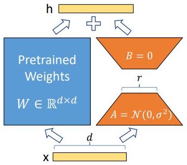
- “Low intrinsic rank” is inspired by the idea of “low intrinsic dimensionality” that these over-parameterized pre-trained models are seen to reside on, and that’s also the explanation behind why fine-tuning only a part of the full model rather than full fine-tuning can yield good results.
- LoRA operates under the hypothesis that the weight changes in the adaptation of a model (fine-tuning) have a low intrinsic rank. In other words, even though a weight matrix may be large, the actual changes made to this matrix during adaptation can be represented in a compressed format, specifically through a low-rank approximation.
- The image below source shows LoRA in action for a diffusion model.
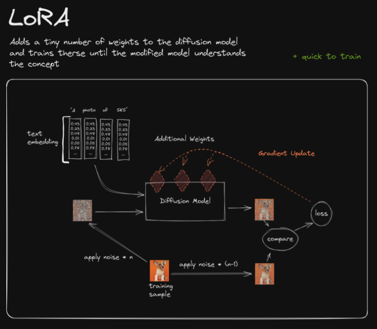
- How LoRA Works:
- Basic Concept: LoRA focuses on adapting only a small fraction of the model’s parameters during fine-tuning. Instead of updating the entire weight matrices in the Transformer layers, it introduces and optimizes low-rank matrices that capture the necessary adaptations for the specific task.
- Modification of Weight Matrices:
- In a standard Transformer model, each layer has weight matrices (like those in the multi-head self-attention and feed-forward networks).
- Rather than directly modifying these weight matrices, LoRA adds trainable low-rank matrices to them. Specifically, for a weight matrix \(W\), the adaptation is done using two smaller matrices \(A\) and \(B\) (where \(A\) and \(B\) are much smaller in size compared to \(W\)).
- The original weight matrix \(W\) remains frozen. During training, the outputs from \(W\) and \(\Delta W = AB\) are added component wise, and the update is effectively: \(W + AB^T\).
- Training Process:
- All we’re now left to optimize is the new matrices \(B\) and \(A\) that contain a very smaller number of parameters (combined) than the full matrix due to their dimensions. Put simply, during training, only the low-rank matrices \(A\) and \(B\) are updated, while the pre-trained weights are kept unchanged.
- In summary, all of the pre-trained weights \(W\) are kept frozen and the rank decomposition matrices of the “change in weight matrix”, \(B\) and \(A\), are optimized. This process reduces the number of trainable parameters significantly, making the fine-tuning process much more efficient in terms of computational resources and time.
- Effectiveness:
- The key to LoRA’s effectiveness lies in the ability of the low-rank matrices to capture the essential changes needed for the new task while leveraging the extensive knowledge already encoded in the pre-trained model.
- Despite updating only a small fraction of parameters, LoRA can achieve performance comparable to full-model fine-tuning on various NLP tasks.
- Advantages of LoRA: LoRA yields significant benefits as compared to full-fine tuning:
- Time and memory Efficiency: Reduces computational and memory costs compared to traditional fine-tuning, where all parameters of the model are updated. With a large percentage of the parameters being frozen, the training time and the GPU memory is saved. Saving is more when using stateful optimizers like Adam, Adadelta, etc.
- Scalability: Enables the adaptation of very large models to specific tasks without prohibitive computational costs.
- Storage efficiency: No need to store huge checkpoints for different downstream tasks. Checkpoint size is greatly reduced with reduction in trainable parameters.
- No additional inference latency: (unlike adapters) just add the learned matrix to the pre-trained one.
- Easy task-switching in deployment: all we need to change is a handful of weights as compared to the full model.
- Preservation of Pre-trained Knowledge: By keeping the majority of the pre-trained weights frozen, LoRA maintains the rich representations learned during pre-training, reducing the risk of catastrophic forgetting.
- Flexibility: Can be applied to different parts of a Transformer model (like attention or feed-forward layers) depending on the task requirements.
- Results:
- With GPT-3 175B, the VRAM consumption during training reduced from 1.2TB to 350GB, while the trained checkpoint size reduced from 350GB to 35MB!
- LoRA achieves performances comparable to and sometimes even better than fine-tuning the full model.
- Applications:
- LoRA is particularly useful for adapting large-scale language models to specific domains or tasks, especially when computational resources are limited or when it’s desirable to maintain the integrity of the pre-trained model while still achieving task-specific performance gains. This approach represents a shift towards more parameter-efficient methods of adapting large models, which is increasingly important as state-of-the-art models continue to grow in size.
What is the difficulty with using the natural gradient (second order gradient) in optimisation rather than the regular gradient descent family (first order)?
- Using the natural gradient, which is a second-order optimization method, in place of the regular gradient descent (a first-order method) presents several challenges and difficulties, particularly in the context of training deep neural networks. Here’s a breakdown of these challenges:
- Computational Complexity:
- Calculation of the Hessian or Fisher Information Matrix:
- Natural gradient descent requires the computation of the Hessian matrix (second-order partial derivatives) or the Fisher Information Matrix. For deep networks with a large number of parameters, this matrix is extremely large and computationally expensive to calculate.
- Inverting the Hessian or Fisher Information Matrix, necessary for natural gradient computations, is computationally intensive and often not feasible for high-dimensional parameter spaces typical in deep learning.
- Calculation of the Hessian or Fisher Information Matrix:
- Memory Requirements:
- Storage Space: Storing the Hessian or Fisher Information Matrix requires a significant amount of memory. For models with millions of parameters, this can quickly become impractical, especially on typical hardware used for training neural networks.
- Numerical Stability:
- Stability and Inversion Issues:
- The Hessian or Fisher Information Matrix can be ill-conditioned, making its inversion numerically unstable. Regularization techniques can be used to mitigate this, but they add additional complexity.
- Approximations to the matrix inversion (like using the matrix inverse lemma) can help but might introduce approximation errors.
- Stability and Inversion Issues:
- Implementation Complexity:
- More Complex Implementation: Implementing natural gradient descent is more complex compared to first-order methods. The simplicity and ease of implementation of first-order methods like stochastic gradient descent (SGD) and its variants (Adam, RMSprop) make them more appealing in practice.
- Efficiency in Deep Learning:
- Efficiency in High-Dimensional Spaces: Despite the theoretical advantages of second-order methods in terms of convergence speed, in practice, first-order methods have shown remarkable efficiency and effectiveness in the high-dimensional spaces characteristic of deep learning.
- Adaptive First-Order Methods: Adaptive gradient methods like Adam partially address some of the issues that natural gradients aim to solve, such as adapting the learning rate to the parameters, making them a more practical choice in many scenarios.
- Applications:
- Niche Applications: Natural gradient methods are more commonly used in specific scenarios where the computational cost is justifiable, such as in smaller models or models where precise convergence is crucial.
- Summary: While natural gradient descent offers theoretical advantages, particularly in terms of faster convergence by taking into account the geometry of the parameter space, its practical application in deep learning is limited due to computational and memory constraints, numerical stability issues, and implementation complexity. In contrast, first-order methods, despite their simplicity, provide a good balance between computational efficiency, ease of use, and performance in large-scale deep learning tasks.
- Computational Complexity:
In the past, CNNs were used for translation. Explain why they are not anymore?
- Convolutional Neural Networks (CNNs) have indeed been used in the past for machine translation tasks, but their prevalence has diminished, especially with the advent of Transformer models. Let’s explore why CNNs are no longer the primary choice for translation:
- - Early Use of CNNs in Translation:
- Feature Extraction: CNNs are effective at extracting local features and recognizing patterns in data, which made them useful in early attempts at neural machine translation.
- Handling Sequences: Initially, CNNs were adapted to handle sequential data by applying convolutions across sequences, capturing local dependencies.
- Shift to RNNs and Then to Transformers:
- Recurrent Neural Networks (RNNs): RNNs, and later LSTMs and GRUs, became more popular for translation due to their inherent ability to handle sequential data and capture long-range dependencies across sentences.
- Introduction of Transformers:
- The introduction of the Transformer model by Vaswani et al. in 2017 marked a significant shift in machine translation. Transformers use self-attention mechanisms, which allow them to process entire sequences of data simultaneously and capture long-range dependencies more effectively than both CNNs and RNNs.
- The parallel processing capability of Transformers significantly improved training efficiency and model performance, making them the de facto choice for machine translation.
- Limitations of CNNs for Translation:
- Local Focus: CNNs are primarily designed to capture local patterns. While they can be stacked to increase their receptive field, they are inherently less efficient at capturing long-range dependencies in sequences compared to self-attention mechanisms.
- Parallelization Limitations: Unlike Transformers, the sequential nature of CNN operations (even when adapted for sequence processing) limits their parallelization capabilities, leading to less efficient training and inference for long sequences.
- Contextual Understanding: CNNs have limitations in their ability to understand the broader context of a sentence, which is crucial in translation for capturing nuances, idiomatic expressions, and context-dependent meanings.
- Conclusion: While CNNs were once a part of the evolving landscape of neural machine translation, the field has progressively moved towards architectures that are more naturally suited to the sequential and context-rich nature of language. The Transformer model, with its superior ability to handle long sequences, context, and parallel processing, has largely supplanted CNNs in this domain. However, it’s worth noting that CNNs still play a vital role in many other areas of deep learning, particularly in image processing and computer vision.
- - Early Use of CNNs in Translation:
Why in Transformers positional encodings are used whereas no such mechanisms are used in RNNs or CNNs. Follow- up: why don’t we use an incremental positional encoding to inform about the positions (1, 2, 3, 4, 5,….), and why do we use sinusoidal functions instead?
- Transformers use positional encodings because, unlike RNNs or CNNs, they lack any inherent mechanism to process data in a sequential order. Each follow-up question addresses specific aspects of this design choice:
- Why Positional Encodings are Used in Transformers:
- Lack of Sequential Processing: In RNNs, the sequential input is inherent in the model’s architecture, as each step’s output depends on the previous step. CNNs, when adapted for sequence processing, also capture local sequence information through their convolutional filters. Transformers, on the other hand, process the entire input sequence simultaneously. This parallel processing is efficient but doesn’t inherently capture the sequential or positional information of the data.
- Preserving Sequence Information: To address this, Transformers add positional encodings to the input embeddings to maintain the order of the sequence. This way, the model can understand the position of each element in the sequence, which is crucial in tasks like language understanding.
- Why Not Use Incremental Positional Encoding:
- Incremental Positional Encoding Limitations:
- Simple incremental encodings (like 1, 2, 3, …) could be used, but they have limitations. They might not scale well with longer sequences, and the model might not generalize well to sequence lengths not seen during training.
- Incremental encodings also do not inherently capture the relative positions of tokens in the sequence.
- Continuous and Relative Position Information:
- Sinusoidal functions provide a way to encode position that allows the model to easily learn to attend by relative positions, as the difference in the encoding between positions is consistent. This is important for generalizing to different sequence lengths and for tasks where relative positioning is crucial.
- The use of sine and cosine functions also ensures that each dimension of the positional encoding varies at a different frequency, making it easier for the model to learn and distinguish between different positions.
- Why Use Sinusoidal Functions:
- Generalization to Longer Sequences: Sinusoidal encodings can be extrapolated and hence allow models to generalize to sequence lengths greater than those encountered during training.
- Encoding Relative Positions: The sine and cosine functions provide a smooth and continuous way to encode positions. They also have the property that their sum/difference can represent relative positions effectively, which is a useful property for understanding language.
- Robustness and Efficiency: Sinusoidal positional encodings add minimal computational complexity and are fixed, not learned, which can provide some stability and reduce overfitting.
- In summary, while Transformers need positional encodings to make sense of the sequence order, the choice of sinusoidal functions is driven by the need for scalability, efficiency, and the ability to capture relative positional information, which are not as effectively addressed by simple incremental encodings.
In diffusion models, there is a forward diffusion process, and a denoising process. For these two processes, when do you use them in training and inference?
- In diffusion models, which are a class of generative models, the forward diffusion process and the denoising process play distinct roles during training and inference. Understanding when and how these processes are used is key to grasping how diffusion models work.
- Forward Diffusion Process
- During Training:
- Noise Addition: In the forward diffusion process, noise is gradually added to the data over several steps or iterations. This process transforms the original data into a pure noise distribution through a predefined sequence of steps.
- Training Objective: The model is trained to predict the noise that was added at each step. Essentially, it learns to reverse the diffusion process.
- During Inference:
- Not Directly Used: The forward diffusion process is not explicitly used during inference. However, the knowledge gained during training (about how noise is added) is implicitly used to guide the denoising process.
- During Training:
- Denoising Process
- During Training:
- Learning to Reverse Noise: The model learns to denoise the data, i.e., to reverse the forward diffusion process. It does this by predicting the noise that was added at each step during the forward diffusion and then subtracting this noise.
- Parameter Optimization: The parameters of the model are optimized to make accurate predictions of the added noise, thereby learning to gradually denoise the data back to its original form.
- During Inference:
- Data Generation: The denoising process is the key to generating new data. Starting from pure noise, the model iteratively denoises this input, using the reverse of the forward process, to generate a sample.
- Iterative Refinement: At each step, the model predicts the noise to remove, effectively refining the sample from random noise into a coherent output.
- During Training:
- Summary
- Training Phase: Both the forward diffusion (adding noise) and the denoising (removing noise) processes are actively used. The model learns how to reverse the gradual corruption of the data (caused by adding noise) by being trained to predict and remove the noise at each step.
- Inference Phase: Only the denoising process is used, where the model starts with noise and iteratively applies the learned denoising steps to generate a sample. The forward process is not explicitly run during inference, but its principles underpin the reverse process.
- Forward Diffusion Process
- In essence, the forward diffusion process is crucial for training the model to understand and reverse the noise addition, while the denoising process is used both in training (to learn this reversal) and in inference (to generate new data).
At a high level, how do diffusion models work? What are some other models that are useful for image generation, and how do they compare to diffusion models?
- Diffusion models, along with Variational Autoencoders (VAEs) and Generative Adversarial Networks (GANs), are powerful tools in the domain of image generation. Each of these models employs distinct mechanisms and has its strengths and limitations.
- How Diffusion Models Work
- Reversible Noising Process:
- Forward Process: Diffusion models work by gradually adding noise to an image (or any data) over a series of steps, transitioning it from the original data distribution to a noise distribution. This process is known as the forward diffusion process.
- Backward Process: The model then learns to reverse this process, which is where the actual generative modeling happens. By learning this reverse diffusion process, the model effectively learns to generate data starting from noise.
- Data Generation: In the generative phase, the model starts with a sample of random noise and applies the learned reverse transformation to this noise, progressively denoising it to generate a sample of data (e.g., an image).
- Higher Quality Samples: Diffusion models are known for generating high-quality samples that are often more realistic and less prone to artifacts compared to other generative models.
- Reversible Noising Process:
- Comparison with VAEs and GANs
- Variational Autoencoders (VAEs):
- Mechanism: VAEs consist of an encoder that maps input data to a latent space and a decoder that reconstructs the data from this latent space. The training involves optimizing the reconstruction loss and a regularization term (KL divergence) that keeps the latent space distributions well-behaved.
- Image Generation: VAEs are effective for image generation but can sometimes produce blurrier results compared to GANs and diffusion models.
- Generative Adversarial Networks (GANs):
- Mechanism: GANs involve a generator that creates images and a discriminator that evaluates them. The generator learns to produce increasingly realistic images, while the discriminator improves at distinguishing real images from generated ones.
- Training Instability: GANs can generate high-quality, sharp images but are known for their training instability issues, such as mode collapse, where the generator produces a limited variety of outputs.
- Comparison to Diffusion Models: Diffusion models, in contrast, generally don’t have these training instabilities and can produce high-quality images, arguably with more consistency than GANs.
- Variational Autoencoders (VAEs):
- Summary
- Diffusion Models: Known for their ability to generate high-quality images and a more stable training process compared to GANs. They work by reversing a learned noising process and are particularly good at capturing fine details in images such as text in generated images, hair follicles as part of a person’s face, etc.
- VAEs: Offer a stable training regime and good general-purpose image generation but sometimes lack the sharpness and realism provided by GANs and diffusion models.
- GANs: Excel in creating sharp and realistic images but can be challenging to train and may suffer from stability issues. Each of these models has its place in the field of image generation, with the choice depending on factors like desired image quality, training stability, and architectural complexity.
What are the loss functions used in Diffusion Models?
- Diffusion models, which are a type of generative model, use a specific approach to learning that involves gradually adding noise to data and then learning to reverse this process. The loss functions used in diffusion models are designed to facilitate this learning process. The primary loss function used is the denoising score matching loss, often combined with other components depending on the specific type of diffusion model.
- Denoising Score Matching Loss
- In diffusion models, the training process involves adding noise to the data in small increments over many steps, resulting in a series of noisier and noisier versions of the original data. The model then learns to reverse this process. The key loss function used in this context is the denoising score matching loss, which can be described as follows:
- Objective: The model is trained to predict the noise that was added to the data at each step. Essentially, it learns how to reverse the diffusion process.
- Implementation: Mathematically, this can be implemented as a regression problem where the model predicts the noise added to each data point. The loss function then measures the difference between the predicted noise and the actual noise that was added. A common choice for this is the mean squared error (MSE) between these two values.
- In diffusion models, the training process involves adding noise to the data in small increments over many steps, resulting in a series of noisier and noisier versions of the original data. The model then learns to reverse this process. The key loss function used in this context is the denoising score matching loss, which can be described as follows:
- Variational Lower Bound (ELBO) in Variational Diffusion Models
- Some diffusion models, particularly variational ones, use a loss function derived from the evidence lower bound (ELBO) principle common in variational inference:
- Objective: This loss function aims to maximize the likelihood of the data under the model while regularizing the latent space representations.
- Components: The ELBO for diffusion models typically includes terms that represent the reconstruction error (similar to the denoising score matching loss) and terms that regularize the latent space (like KL divergence in VAEs).
- Some diffusion models, particularly variational ones, use a loss function derived from the evidence lower bound (ELBO) principle common in variational inference:
- Additional Regularization Terms
- Depending on the specific architecture and objectives of the diffusion model, additional regularization terms might be included:
- KL Divergence: In some models, especially those that involve variational approaches, a KL divergence term can be included to ensure that the learned distributions in the latent space adhere to certain desired properties.
- Adversarial Loss: For models that integrate adversarial training principles, an adversarial loss term might be added to encourage the generation of more realistic data.
- Depending on the specific architecture and objectives of the diffusion model, additional regularization terms might be included:
- Summary: The choice of loss function in diffusion models is closely tied to their unique training process, which involves learning to reverse a controlled noise-adding process. The denoising score matching loss is central to this, often supplemented by other loss components based on variational principles or additional regularization objectives. The combination of these loss functions allows diffusion models to effectively learn the complex process of generating high-quality data from noisy inputs.
What is the Denoising Score Matching Loss in Diffusion models? Provide equation and intuition.
- The Denoising Score Matching Loss is a critical component in the training of diffusion models, a class of generative models. This loss function is designed to train the model to effectively reverse a diffusion process, which gradually adds noise to the data over a series of steps.
- Denoising Score Matching Loss: Equation and Intuition
- Background:
- In diffusion models, the data is incrementally noised over a sequence of steps. The reverse process, which the model learns, involves denoising or reversing this noise addition to recreate the original data from noise.
- Equation:
- The denoising score matching loss at a particular timestep \(t\) can be formulated as:
\(L(\theta)=\mathbb{E}_{x_0, \epsilon \sim \mathcal{N}(0, I), t}\left[\left\|s_\theta\left(x_t, t\right)-\nabla_{x_t} \log p_{t \mid 0}\left(x_t \mid x_0\right)\right\|^2\right]\)
- where, \(x_0\) is the original data, \(x_t\) is the noised data at timestep \(t\), and $\epsilon$ is the added Gaussian noise.
- \(s_\theta\left(x_t, t\right)\) is the score (gradient of the log probability) predicted by the model with parameters \(\theta\).
- \(\nabla_{x_t} \log p_{t \mid 0}\left(x_t \mid x_0\right)\) is the true score, which is the gradient of the log probability of the noised data \(x_t\) conditioned on the original data \(x_0\).
- Intuition:
- The loss function encourages the model to predict the gradient of the log probability of the noised data with respect to the data itself. Essentially, it’s training the model to estimate how to reverse the diffusion process at each step.
- By minimizing this loss, the model learns to approximate the reverse of the noising process, thereby learning to generate data starting from noise.
- This process effectively teaches the model the denoising direction at each step of the noised data, guiding it on how to gradually remove noise and reconstruct the original data.
- Importance in Training: The denoising score matching loss is crucial for training diffusion models to generate high-quality samples. It ensures that the model learns a detailed and accurate reverse mapping of the diffusion process, capturing the complex data distribution.
- Advantages: This approach allows diffusion models to generate samples that are often of higher quality and more diverse compared to other generative models, as it carefully guides the generative process through the learned noise reversal.
- Background:
- In summary, the denoising score matching loss in diffusion models is fundamental in training these models to effectively reverse the process of gradual noise addition, enabling the generation of high-quality data samples from a noise distribution. This loss function is key to the model’s ability to learn the intricate details of the data distribution and the precise dynamics of the denoising process.
At a high level, what is RLHF? Why is this a novel paradigm compared to, for example, self-supervised learning on an uncurated text corpus? What does alignment mean in the context of LLMs?
- RLHF, short for Reinforcement Learning from Human Feedback, is an advanced machine learning paradigm that significantly differs from traditional training methods like using uncurated text corpora. This approach is particularly relevant in the context of training language models, where aligning the model’s output with human values and preferences is crucial.
- High-Level Overview of RLHF
- Integration of Human Feedback: RLHF involves training models, particularly reinforcement learning models, using feedback derived from human interactions or evaluations. Instead of solely relying on pre-existing datasets or unstructured text, RLHF utilizes human-generated feedback to guide the learning process.
- Fine-Tuning on Human Rankings:
- In this approach, the model is fine-tuned based on human judgments or rankings of its outputs. For example, humans may evaluate a set of responses or actions generated by the model and rank them according to their relevance, quality, or alignment with specific criteria.
- The model then uses these rankings to adjust its parameters, essentially learning to prefer actions or outputs that are more highly ranked by humans.
- Novelty and Advantages of RLHF Compared to Uncurated Text Corpora
- Better Human Alignment:
- RLHF allows for the creation of models that are better aligned with human values, preferences, and nuances of judgment; for e.g., safe, helpful, adheres to guidelines and constraints. This is particularly important in applications where ethical, cultural, or subjective considerations play a significant role.
- Traditional models trained on uncurated text corpora may inadvertently learn and amplify biases, inaccuracies, or undesirable behaviors present in the training data.
- Better Human Alignment:
- Customized and Targeted Learning: - With RLHF, the learning process is more targeted and customized to specific goals or standards set by humans. This is in contrast to the more generalized learning from uncurated corpora, which might not be tailored to specific use-cases or quality standards.
- Improved Performance in Complex Tasks: - RLHF can lead to improved performance in complex tasks, especially those that require understanding of context, subtlety, and nuances that are not easily captured by standard datasets but are understandable to humans.
- Flexibility and Adaptability: - This approach offers flexibility, as the criteria for human feedback can be adjusted based on the desired outcome. It allows the model to adapt to evolving standards or preferences over time.
- Conclusion RLHF represents a novel paradigm in machine learning by directly incorporating human feedback into the training process. This method addresses some of the limitations of training on unstructured text corpora, particularly in terms of aligning AI behavior with human values and expectations. By fine-tuning models based on human rankings and feedback, RLHF fosters the development of AI systems that are not only technically proficient but also ethically and contextually aware, catering to more nuanced and human-centric applications.
Can you please describe the structure of CNNs? The different layers, activation functions? What are some key properties of activation functions?
- Convolutional Neural Networks (CNNs) are a class of deep neural networks widely used in processing data with a grid-like topology, such as images. They are known for their ability to detect hierarchical patterns in data. Here’s an overview of their structure, including layers and activation functions:
- Structure of CNNs
- Convolutional Layers: These layers apply a set of learnable filters (kernels) to the input. Each filter convolves across the width and height of the input volume, computing the dot product between the filter and input, producing a 2D activation map.
- Key Property: Convolutional layers are adept at capturing spatial hierarchies in images by learning from local regions (like edges, textures) in the early layers and more complex patterns (like objects, shapes) in deeper layers.
- Pooling Layers: Often placed after convolutional layers, pooling layers (such as max pooling or average pooling) reduce the spatial dimensions (width and height) of the input volume, leading to a reduction in the number of parameters and computation in the network. Key Property: Pooling helps in making the detection of features invariant to scale and orientation changes.
- Fully Connected Layers: At the end of the network, one or more fully connected layers are used where each neuron is connected to all neurons in the previous layer. These layers are typically used for classifying the features learned by the convolutional layers into different classes.
- Key Property: Fully connected layers combine features to make final predictions.
- Dropout: Dropout is a regularization technique used in CNNs to prevent overfitting. It randomly “drops” a subset of neurons in a layer during training, forcing the network to learn redundant representations and enhancing its generalization capabilities.
- Batch Normalization: Batch normalization is a technique to stabilize and accelerate the training of deep networks. It normalizes the activations of a previous layer at each batch, i.e., it applies a transformation that maintains the mean activation close to 0 and the activation standard deviation close to 1.
- Activation Functions
- 1. ReLU (Rectified Linear Unit):
- Formula: $f(x)=\max (0, x)$
- Properties: Non-linear, allows models to account for complex data patterns; simple and efficient in computation.
- Variants like Leaky ReLU or Parametric ReLU are used to address the “dying ReLU” problem where neurons can become inactive and stop contributing to the learning process.
- 2. Sigmoid:
- Formula: $\sigma(x)=\frac{1}{1+e^{-x}}$
- Properties: Smooth gradient, squashing values into a range between 0 and 1 . It’s often used in the output layer for binary classification.
- 3. Tanh (Hyperbolic Tangent):
- Formula: $\tanh (x)=\frac{e^x-e^{-x}}{e^x+e^{-x}}$
- Properties: Similar to sigmoid but squashes values into a range between -1 and 1 . It is zerocentered, making it easier to model inputs that have strongly negative, neutral, and strongly positive values.
- Softmax: Used in the output layer of a CNN for multi-class classification; it turns logits into probabilities that sum to one.
- Properties: Softmax is non-linear and is able to handle multiple classes in a mutually exclusive scenario.
- 1. ReLU (Rectified Linear Unit):
- Key Properties of Activation Functions
- Nonlinearity: This allows CNNs to capture complex relationships in data. Without nonlinearity, the network would behave like a linear model.
- Differentiability: Essential for enabling backpropagation where gradients are computed during training.
- Computational Efficiency: Faster activation functions (like ReLU) lead to quicker training.
- In summary, the structure of CNNs, characterized by alternating convolutional and pooling layers followed by fully connected layers, combined with dropout for regularization and batch normalization for faster training, is optimized for feature detection and classification. The choice of activation function, critical for introducing nonlinearity, depends on the specific requirements of the task and the network architecture.
What are some differences between a CNN and a FCNN? Layers and activation functions? Why are they structured differently?
- The terms CNN (Convolutional Neural Network) and FCNN (Fully Convolutional Neural Network) refer to specific architectures within the realm of neural networks, each with distinct characteristics tailored to different types of tasks.
- CNN (Convolutional Neural Network)
- Structure:
- Convolutional Layers: CNNs use convolutional layers, where filters are applied to the input to create feature maps. These filters detect local features like edges, textures, etc.
- Pooling Layers (e.g., Max Pooling): Following convolutional layers, pooling layers reduce the spatial dimensions (width and height) of the feature maps, helping in achieving spatial invariance to input translations.
- Fully Connected Layers: Towards the end, CNNs typically have one or more fully connected layers. Here, neurons have connections to all activations in the previous layer, as seen in traditional neural networks.
- Activation Functions: Commonly use ReLU or variants like Leaky ReLU; also employ softmax in the output layer for classification tasks.
- Parameter Sharing and Spatial Invariance:
- The use of convolutional filters involves parameter sharing, reducing the total number of parameters and making the network efficient at learning spatial hierarchies.
- Pooling layers contribute to spatial invariance, making the network robust to variations in the location of features in the input.
- FCNN (Fully Convolutional Neural Network)
- Structure:
- Only Convolutional Layers: FCNNs, as the name suggests, are composed entirely of convolutional layers. They do not have any fully connected layers.
- Upsampling Layers: In tasks like semantic segmentation, FCNNs use upsampling techniques (like transposed convolutions) to increase the spatial resolution of feature maps.
- Activation Functions: Similar to CNNs, FCNNs use activation functions like ReLU in convolutional layers.
- Designed for Spatial Data:
- FCNNs are designed for tasks where the spatial dimension of the output is crucial, like in image segmentation, where an output pixel-wise map is needed.
- They maintain spatial information throughout the network, which is lost in the fully connected layers of CNNs.
- Differences and Structural Reasons
- Max Pooling and Fully Connected Layers in CNNs:
- These components are used in CNNs for classification tasks where the goal is to identify global features or patterns in the entire input (like identifying objects in images).
- Max Pooling helps in reducing the dimensionality and provides translation invariance, beneficial for classification tasks.
- Absence of Fully Connected Layers in FCNNs:
- FCNNs are structured to maintain spatial information, which is essential for tasks like segmentation where the exact location of objects in an image is important.
- The absence of fully connected layers allows FCNNs to accept inputs of any size and produce correspondingly-sized outputs.
- Structure:
- Conclusion
- CNNs are typically used for classification tasks. They leverage the spatial invariance property with max pooling and parameter sharing in filters, followed by fully connected layers for high-level reasoning.
- FCNNs are used primarily for spatially-oriented tasks like segmentation. They maintain spatial dimensions throughout the network, allowing for precise, pixel-level predictions.
- The choice between CNN and FCNN depends on the specific requirements of the task, particularly regarding the importance of preserving spatial information in the output.
What are some differences between a CNN and a FFNN? Layers and activation functions? Why are they structured differently?
- Convolutional Neural Networks (CNNs) and Fully Connected Neural Networks (FCNNs) differ significantly in their structures, purposes, and the specific tasks they are best suited for. Here are some of the key differences:
- CNN (Convolutional Neural Network)
- Structure: Convolutional Layers: CNNs primarily consist of convolutional layers, where filters or kernels are convolved with the input data to extract features.
- Pooling Layers (Max Pooling): Pooling layers, such as max pooling, are used to reduce the spatial dimensions of the feature maps. This operation helps in achieving spatial invariance to input translations and reducing the number of parameters.
- Parameter Sharing: In convolutional layers, the same filter is applied across different parts of the input, significantly reducing the number of parameters compared to a fully connected architecture.
- Spatial Invariance:
- CNNs leverage the spatial invariance property, meaning they can detect features regardless of their spatial location in the input data.
- This property makes CNNs particularly suited for tasks like image recognition, where the exact location of a feature (like an edge or a shape) is less important than its presence.
- Activation Functions:
- Commonly use ReLU (Rectified Linear Unit) or its variants like Leaky ReLU for introducing non-linearity.
- The output layer may use softmax for multi-class classification tasks.
- FCNN (Fully Connected Neural Network)
- Structure:
- Fully Connected Layers: In a fully connected neural network, every neuron in one layer is connected to every neuron in the next layer. This means the number of parameters can be quite large, especially for networks with many neurons.
- No Spatial Invariance: Fully connected layers do not inherently have spatial invariance. They treat input data as a flat vector of features without considering the spatial relationships between them.
- Use Cases: FCNNs are more general-purpose and can be used for a wide range of tasks, including classification and regression. However, they are not specialized for spatial data like images.
- Activation Functions: Similar to CNNs, FCNNs can use a variety of activation functions like ReLU, sigmoid, or tanh, depending on the specific application.
- Structure:
- Key Differences and Rationale
- Max Pooling in CNNs: Max pooling reduces the spatial dimensions of feature maps, enhancing the network’s ability to capture important features regardless of their position. This is particularly useful for image data where nearby pixels are more related.
- Parameter Efficiency in CNNs: The use of convolutional layers with parameter sharing and pooling layers in CNNs minimizes the number of parameters needed, making them more efficient for image-related tasks.
- FC Layers in CNNs: While CNNs often end with one or more fully connected layers for classification, these come after convolutional and pooling layers have extracted spatial features.
- CNN (Convolutional Neural Network)
- In summary, CNNs are structured to exploit the spatial relationships inherent in data like images, using fewer parameters through convolutional layers and achieving spatial invariance with pooling layers. In contrast, fully connected networks are more general-purpose and lack these spatial efficiencies, making them less suitable for tasks like image recognition but useful for other types of data-driven tasks.
Imagine you are designing a CNN from scratch. How would you think about choosing the CNN kernel size? What are some considerations?
- Designing a Convolutional Neural Network (CNN) from scratch involves several important decisions, one of which is choosing the kernel size for the convolutional layers. The kernel size can significantly impact the network’s performance, computational efficiency, and its ability to capture relevant features from the input data. Here are some considerations for choosing the CNN kernel size:
- Larger Kernels
- More Parameters and Computational Complexity: Larger kernels (e.g., 5x5, 7x7) have more parameters. This increases the computational complexity and the memory footprint of the model.
- Capturing Global Information: They are capable of capturing more global information in the input data. For example, a larger kernel can cover a larger area of the input image, thus encapsulating more global features at once.
- Suitability: Larger kernels might be more suitable for tasks where understanding broader patterns is important, such as in detecting general shapes or configurations in an image.
- Smaller Kernels
- Fewer Parameters and Lower Computational Complexity: Smaller kernels (e.g., 3x3, 1x1) have fewer parameters, making the network computationally more efficient and reducing the risk of overfitting.
- Capturing Fine Details:
- They excel at capturing fine-grained details in the input. This is crucial for tasks where local features are important, such as in texture analysis or detecting small objects.
- Stacking Layers for Larger Receptive Fields:
- Stacking multiple layers of small kernels can effectively increase the receptive field, similar to a single layer of a larger kernel, but with fewer parameters and potentially better feature extraction due to the increased depth.
- Task-Specific Considerations
- Type of Task - Broad Patterns vs. Fine Details: The choice of kernel size should align with the nature of the task. For instance, if the task requires understanding broad patterns (like in scene recognition), larger kernels may be more appropriate. Conversely, for tasks focusing on finer details (like in medical imaging for detecting small anomalies), smaller kernels could be more effective.
- Computational Resources
- Resource Constraints: The availability of computational resources also plays a role. Larger kernels may not be feasible in resource-constrained environments due to their higher computational demands.
- Combining Different Kernel Sizes
- Hybrid Approaches: Some advanced CNN architectures use a combination of different kernel sizes in parallel branches (like in Inception networks) to capture both local and global features effectively.
- Larger Kernels
- Conclusion: In summary, choosing the kernel size in a CNN is a balance between capturing broad/global patterns vs. fine-grained features, computational efficiency, and the specific requirements of the task at hand. Smaller kernels are generally preferred for their efficiency and ability to capture detailed features, especially when used in deeper architectures. However, larger kernels have their place in scenarios where broader feature extraction is crucial. Often, a combination of different kernel sizes, either sequentially or in parallel, can provide a comprehensive feature extraction mechanism suitable for a wide range of tasks.
Both a fully-connected layer and a self-attention layer allow for all-to-all interactions. What is the advantage of a self-attention layer?
- Fully connected layers and self-attention layers both enable all-to-all interactions among their inputs, but they do so in fundamentally different ways, each offering unique advantages. The self-attention layer, especially as used in Transformer models, has several key benefits:
- Advantages of Self-Attention Layer
- Interpretability via Attention Scores:
- Mechanism:Self-attention mechanisms compute attention scores representing the influence or ‘attention’ each input element should receive from other elements.
- Advantage: These attention scores provide a form of interpretability. By examining the attention scores, one can understand the relationships and dependencies the model is inferring between different parts of the input. For instance, in language models, this can show which words or phrases the model considers relevant when processing a given word.
- Parameter Efficiency in Some Cases:
- Comparison with Fully Connected Layers: Fully connected layers have a separate parameter for each connection between neurons in adjacent layers. This can lead to a very high number of parameters, especially in large networks.
- Self-Attention Efficiency: In contrast, self-attention layers use query (Q), key (K), and value (V) matrices to compute attention scores. The number of parameters in these matrices does not directly depend on the input size but rather on the chosen embedding size (dimensionality of Q, K, and V). This can lead to fewer parameters when the embedding size is smaller than the input size.
- Handling Variable-Length Input:
- Flexibility: Self-attention layers are inherently suited for variable-length input, such as sentences in natural language processing, which can vary in length.
- Implementation: Since attention is computed pairwise between elements (e.g., words in a sentence), it naturally adapts to the length of the input. In contrast, fully connected layers require a fixed-size input, and adapting them to variable-length data often involves additional mechanisms like padding or truncation.
- Additional Considerations
- Computational Efficiency: While self-attention can be more parameter-efficient, it can also be computationally intensive, especially for very long sequences, as the computation grows quadratically with sequence length.
- Global Context: Self-attention layers can capture global dependencies in the input data, as each output element is a function of all input elements. This is particularly advantageous in tasks like language understanding, where context is crucial.
- Conclusion Self-attention layers offer interpretability through attention scores, can be more parameter-efficient depending on the embedding size, and are naturally adaptable to variable-length inputs. These qualities make them particularly powerful in applications like language processing and sequence modeling, where context and relationships between input elements are key to effective modeling.
- Interpretability via Attention Scores:
What is the advantage of using a self-attention-based ViT model compared to using fully CNN layers?
- ViT stands for Vision Transformer, a model that applies the Transformer architecture, typically used in natural language processing (NLP), to computer vision tasks. This model, introduced by researchers at Google, represents a significant shift in the approach to image processing tasks, traditionally dominated by Convolutional Neural Networks (CNNs).
- What’s Interesting About ViT?
- Application of Transformers to Images: ViT adapts the Transformer architecture, which was originally designed for sequence-to-sequence tasks like language translation, to handle image data. It treats images not as 2D grids of pixels but as sequences of flattened image patches.
- Patch-Based Image Processing: An image in ViT is divided into fixed-size patches, which are then linearly embedded (similar to word embeddings in NLP). These embedded patches are treated as tokens in a sequence, making the Transformer’s self-attention mechanism applicable to them.
- Global Context: Unlike CNNs, which process local receptive fields, the self-attention mechanism in ViT allows each patch to attend to all other patches. This enables the model to capture global context in the image, potentially leading to a richer understanding of the scene.
- Advantages of Transformer-Based Self-Attention in Vision Models
- Capturing Long-Range Dependencies: Self-attention allows the model to capture relationships between distant parts of the image in a way that CNNs, with their local receptive fields, cannot easily achieve. This is beneficial for understanding complex scenes where the context is important.
- Flexibility and Scalability: The Transformer architecture is inherently scalable and can be effectively trained on large datasets. ViT, in particular, has shown impressive performance gains when trained on very large image datasets.
- Reduced Inductive Bias: CNNs come with a strong inductive bias towards spatial hierarchies and locality, which is generally beneficial for image data but can also limit their flexibility. Transformers, having less inductive bias, can learn different types of representations depending on the task and data.
- Efficiency with Larger Images: For large images, the ability of self-attention to process the entire image at once can be computationally more efficient than the sliding window approach of CNNs.
- Considerations
- Data and Compute Intensive: ViT models tend to require significant amounts of data and computational resources to outperform CNNs, particularly on smaller datasets or less complex tasks where the inductive biases of CNNs are advantageous.
- Positional Encodings: Just like in NLP, positional encodings are used in ViT to retain information about the position of patches in the image.
- In summary, the Vision Transformer presents an innovative approach to image processing, leveraging the global receptive fields and scalability of the Transformer architecture. It has opened up new possibilities in computer vision, particularly for tasks where understanding the global context is crucial. However, the trade-offs in terms of data and computational requirements need to be considered when choosing between ViT and traditional CNN-based approaches.
What is self-supervised learning? Can you give some examples of self-supervised learning paradigms?
- Self-supervised learning is a subset of unsupervised learning, which has gained significant traction in machine learning, particularly in fields like natural language processing (NLP) and computer vision. This approach involves using the data itself to generate supervisory signals, effectively creating a learning task without the need for externally labeled data.
- Overview of Self-Supervised Learning
- Data as its Own Supervisor: In self-supervised learning, algorithms generate labels from the data itself. The model is tasked with predicting some part of the data using other parts of the same data as context, thus leveraging the inherent structure within the data for learning.
- Automatic Label Generation: The key aspect of this approach is that it doesn’t rely on human-annotated labels. Instead, it auto-generates labels, making it scalable and less reliant on often expensive and time-consuming manual labeling processes.
- Examples of Self-Supervised Learning Paradigms
- Contrastive Learning:
- SimCLR, MoCo: These are frameworks used primarily in computer vision. They involve creating positive pairs of augmented samples from the same original image and negative pairs from different images. The learning task is to bring the representations of positive pairs closer together while pushing the negative pairs apart. This approach helps the model learn robust feature representations that are invariant to the augmentations.
- Key Idea: By learning to identify which samples are similar or ‘positive’ (augmentations of the same image) and which are ‘negative’ (different images), the model develops an understanding of the essential features and patterns in the visual data.
- Masked Language Modeling (MLM):
- BERT in NLP: In this paradigm, used in models like BERT, certain words in the input text are masked, and the model’s task is to predict these masked words. This forces the model to understand context and relationships between words.
- Vision Models: A similar approach can be applied to vision, where parts of an image are masked, and the model learns to predict these missing parts, thereby understanding the structure and content of the visual data.
- Key Characteristics and Advantages
- Learning Rich Representations: Self-supervised learning enables models to learn rich representations of data, capturing underlying structures and relationships without explicit external labels.
- Scalability: Since it doesn’t require labeled data, self-supervised learning can be applied to much larger datasets, making it highly scalable.
- Versatility: It is versatile and can be applied to various types of data, including text, images, and audio.
- Conclusion: Self-supervised learning represents a powerful paradigm in modern machine learning, particularly useful in situations where labeled data is scarce or expensive to obtain. By creatively using the data itself to generate learning tasks, self-supervised learning models can uncover complex patterns and relationships within the data, leading to robust and generalizable representations. This approach has been instrumental in recent advances in fields like NLP and computer vision, demonstrating the potential of learning from large amounts of unlabeled data.
Did the original Transformer use absolute or relative positional encoding?
- The original Transformer model, as introduced by Vaswani et al. in their 2017 paper “Attention Is All You Need”, used absolute positional encoding. This design was a key feature to incorporate the notion of sequence order into the model’s architecture.
- Absolute Positional Encoding in the Original Transformer
- Mechanism:
- The Transformer model does not inherently capture the sequential order of the input data in its self-attention mechanism. To address this, the authors introduced absolute positional encoding.
- Each position in the sequence was assigned a unique positional encoding vector, which was added to the input embeddings before they were fed into the attention layers.
- Implementation: The positional encodings used were fixed (not learned) and were based on sine and cosine functions of different frequencies. This choice was intended to allow the model to easily learn to attend by relative positions since for any fixed offset \(k, PE_{pos + k}\) could be represented as a linear function of \(PE_{pos}\).
- Mechanism:
- Importance: This approach to positional encoding was crucial for enabling the model to understand the order of tokens in a sequence, a fundamental aspect of processing sequential data like text.
- Relative and Rotary Positional Encoding in Later Models
- After the introduction of the original Transformer, subsequent research explored alternative ways to incorporate positional information. One such development was the use of relative positional encoding, which, instead of assigning a unique encoding to each absolute position, encodes the relative positions of tokens with respect to each other. This method has been found to be effective in certain contexts and has been adopted in various Transformer-based models developed after the original Transformer. Rotary positional encoding methods (such as RoPE) were also presented after relative positional encoding methods.
- Conclusion: In summary, the original Transformer model utilized absolute positional encoding to integrate sequence order into its architecture. This approach was foundational in the development of Transformer models, while later variations and improvements, including relative positional encoding, have been explored in subsequent research to further enhance the model’s capabilities.
How does the choice of positional encoding method can influence the number of parameters added to the model? Consinder absolute, relative, and rotary positional encoding mechanisms.
- In Large Language Models (LLMs), the choice of positional encoding method can influence the number of parameters added to the model. Let’s compare absolute, relative, and rotary (RoPE) positional encoding in this context:
- Absolute Positional Encoding
- Parameter Addition:
- Absolute positional encodings typically add a fixed number of parameters to the model, depending on the maximum sequence length the model can handle.
- Each position in the sequence has a unique positional encoding vector. If the maximum sequence length is \(N\) and the model dimension is \(D\), the total number of added parameters for absolute positional encoding is \(N \times D\).
- Fixed and Non-Learnable: In many implementations (like the original Transformer), these positional encodings are fixed (based on sine and cosine functions) and not learnable, meaning they don’t add to the total count of trainable parameters.
- Parameter Addition:
- Relative Positional Encoding
- Parameter Addition:
- Relative positional encoding often adds fewer parameters than absolute encoding, as it typically uses a set of parameters that represent relative positions rather than unique encodings for each absolute position.
- The exact number of added parameters can vary based on the implementation but is generally smaller than the \(N \times D\) parameters required for absolute encoding.
- Learnable or Fixed: Depending on the model, relative positional encodings can be either learnable or fixed, which would affect whether they contribute to the model’s total trainable parameters.
- Parameter Addition:
- Rotary Positional Encoding (RoPE)
- Parameter Addition:
- RoPE does not add any additional learnable parameters to the model. It integrates positional information through a rotation operation applied to the query and key vectors in the self-attention mechanism.
- The rotation is based on the position but is calculated using fixed, non-learnable trigonometric functions, similar to absolute positional encoding.
- Efficiency: The major advantage of RoPE is its efficiency in terms of parameter count. It enables the model to capture relative positional information without increasing the number of trainable parameters.
- Parameter Addition:
- Summary:
- Absolute Positional Encoding: Adds \(N \times D\) parameters, usually fixed and non-learnable.
- Relative Positional Encoding: Adds fewer parameters than absolute encoding, can be learnable, but the exact count varies with implementation.
- Rotary Positional Encoding (RoPE): Adds no additional learnable parameters, efficiently integrating positional information.
- In terms of parameter efficiency, RoPE stands out as it enriches the model with positional awareness without increasing the trainable parameter count, a significant advantage in the context of LLMs where managing the scale of parameters is crucial.
In LLMs, why is RoPE required for context length extension?
- RoPE, or Rotary Positional Embedding, is a technique used in some language models, particularly Transformers, for handling positional information. The need for RoPE or similar techniques becomes apparent when dealing with long context lengths in Large Language Models (LLMs).
- Context Length Extension in LLMs
- Positional Encoding in Transformers:
- Traditional Transformer models use positional encodings to add information about the position of tokens in a sequence. This is crucial because the self-attention mechanism is, by default, permutation-invariant (i.e., it doesn’t consider the order of tokens).
- In standard implementations like the original Transformer, positional encodings are added to the token embeddings and are typically fixed (not learned) and based on sine and cosine functions of different frequencies.
- Challenges with Long Sequences: As the context length (number of tokens in a sequence) increases, maintaining effective positional information becomes challenging. This is especially true for fixed positional encodings, which may not scale well or capture relative positions effectively in very long sequences.
- Role and Advantages of RoPE
- Rotary Positional Embedding: RoPE is designed to provide rotational equivariance to self-attention. It essentially encodes the absolute position and then rotates the positional encoding of keys and queries differently based on their position. This allows the model to implicitly capture relative positional information through the self-attention mechanism.
- Effectiveness in Long Contexts: RoPE scales effectively with sequence length, making it suitable for LLMs that need to handle long contexts or documents. This is particularly important in tasks like document summarization or question-answering over long passages.
- Preserving Relative Positional Information: RoPE allows the model to understand the relative positioning of tokens effectively, which is crucial in understanding the structure and meaning of sentences, especially in languages with less rigid syntax.
- Computational Efficiency: Compared to other methods of handling positional information in long sequences, RoPE can be more computationally efficient, as it doesn’t significantly increase the model’s complexity or the number of parameters.
- Conclusion: In summary, RoPE is required for effectively extending the context length in LLMs due to its ability to handle long sequences while preserving crucial relative positional information. It offers a scalable and computationally efficient solution to one of the challenges posed by the self-attention mechanism in Transformers, particularly in scenarios where understanding the order and relationship of tokens in long sequences is essential.
Is multicollinearity and correlation the same?
- Multicollinearity and correlation, while related concepts, are not the same. They both deal with relationships between variables in statistical analyses, but they differ in their specific focus and implications:
- Correlation:
- Correlation refers to any of a broad class of statistical relationships involving dependence between two variables.
- The most common measure of correlation is the Pearson correlation coefficient, which assesses the linear relationship between two variables.
- Correlation can be positive (both variables increase or decrease together), negative (one variable increases while the other decreases), or zero (no linear relationship).
- Correlation is a bivariate (two-variable) concept.
- Multicollinearity:
- Multicollinearity refers specifically to a situation in regression analysis where two or more predictors (independent variables) are highly correlated.
- This means that one predictor variable in a multiple regression model can be linearly predicted from the others with a substantial degree of accuracy.
- Multicollinearity can make it difficult to ascertain the effect of each predictor on the dependent variable, as changes in one predictor are associated with changes in another.
- It is a problem in multiple regression models, as it undermines the statistical significance of an independent variable.
- Correlation:
- In summary, while correlation is a broader concept that describes the linear relationship between two variables, multicollinearity is a more specific situation where two or more variables in a regression model are highly correlated, potentially causing issues in interpreting the model results.
Do you need a non-linearity such as ReLU or sigmoid at the last layer of a neural network?
- Suppose you have \(N\) hidden layers, and the output layer is just a softmax layer over a set of neurons representing classes (so the expected output is the probability that the input data belongs to each class). Assuming the first \(N-1\) layers have nonlinear neurons, should you use a non-linearity in the \(N^{th}\) hidden layer.
- You should not use a non-linearity for the last layer before the softmax classification. The ReLU non-linearity (used now almost exclusively) will in this case simply throw away information without adding any additional benefit. You can look at the caffe implementation of the well-known AlexNet for a reference of what’s done in practice.
- Note that the softmax function is already non-linear. The softmax function converts a vector of real numbers into a probability distribution. The output probabilities of the softmax function are computed by exponentiating each input value, making it non-negative, and then normalizing by the sum of these exponentiated values across the vector. This non-linearity is particularly useful in classification problems where it helps to distinguish between different classes by amplifying the differences in the input values, thus making the output more distinct for each class.
- Credit for this answer go to Non-linearity before final Softmax layer in a convolutional neural network.
Explain the concept of temperature in deep learning?
-
In deep learning, the concept of “temperature” is often associated with the Softmax function and is used to control the degree of confidence or uncertainty in the model’s predictions. It’s primarily applied in the context of classification tasks, such as image recognition or natural language processing, where the model assigns probabilities to different classes.
-
The Softmax function is used to convert raw model scores or logits into a probability distribution over the classes. Each class is assigned a probability score, and the class with the highest probability is typically selected as the predicted class.
-
The Softmax function is defined as follows for a class “i”:
-
Where:
- \(P(i)\) is the probability of class “i.”
- \(z_i\) is the raw score or logit for class “i.”
-
\(\tau\), known as the “temperature,” is a positive scalar parameter.
-
The temperature parameter, \(\tau\), affects the shape of the probability distribution. When \(\tau\) is high, the distribution becomes “soft,” meaning that the probabilities are more evenly spread among the classes. A lower temperature results in a “harder” distribution, with one or a few classes having much higher probabilities.
-
Here’s how temperature impacts the Softmax function:
- High \(\tau\): The model is more uncertain, and the probability distribution is more uniform, which can be useful when exploring diverse options or when dealing with noisy data.
- Low \(\tau\): The model becomes more confident, and the predicted class will have a much higher probability. This is useful when you want to make decisive predictions.
- Temperature allows you to control the trade-off between exploration and exploitation in the model’s predictions. It’s a hyperparameter that can be adjusted during training or inference to achieve the desired level of certainty in the model’s output, depending on the specific requirements of your application.
What is the difference between logits, soft and hard targets?
- Let us understand each of the terms one by one. For better understanding, let’s take a dog vs cat image classification as an example.
- Logits are the un-normalized output of the model. In our cat vs dog example, logits will be, say,
10.1for cat and5.6for dog for an image with cat. Refer this SE question. - Soft target: are normalized logits by applying a softmax function [(without a non-linearity such as ReLU or sigmoid)]](https://stats.stackexchange.com/questions/163695/non-linearity-before-final-softmax-layer-in-a-convolutional-neural-network). In our example, if we use softmax to the logits we get
0.99for cat and0.1for dog. - Hard targets: are the encoding of the soft targets. In our example, as the model predicted (here correctly) the image as of cat, the hard targets be
1for cat and0for dog.
- Logits are the un-normalized output of the model. In our cat vs dog example, logits will be, say,
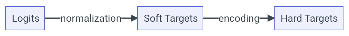
What is Deep Learning and How is it Different from Traditional Machine Learning?
- Deep Learning is a specialized subfield of machine learning focusing on neural networks with multiple layers, aptly termed deep neural networks.
- These networks excel in learning and making predictions by autonomously identifying hierarchical data representations, distinguishing them from traditional machine learning, which relies more on manual feature engineering.
- Deep learning models are particularly adept at handling unstructured data like images and text, making them suitable for complex tasks like image recognition and natural language processing.
How Does Backpropagation Work in a Neural Network?
- Backpropagation is a cornerstone algorithm in training neural networks, pivotal for their ability to learn and adjust.
- It begins by forwarding the input through the network to compute the output.
- The algorithm then assesses the output against the expected result, calculating the error.
- This error is propagated backward through the network, adjusting the weights to minimize this error.
- The process iteratively repeats, refining the network’s performance by reducing the error.
Why Do We Prefer Training on Mini-Batches Rather Than Individual Samples in Deep Learning?
- Mini-batch training strikes a balance between computational efficiency and estimation quality.
- The gradient calculated over a mini-batch is an estimation of the gradient over the entire training set, improving with larger batch sizes.
- Moreover, processing a batch of data simultaneously leverages modern computing architectures’ parallelism, offering significant efficiency over handling each data point separately.
What are the Benefits of Using Batch Normalization?
- Batch Normalization significantly impacts the gradient flow within a network, reducing dependency on the parameters’ scale or their initial values.
- This feature enables the use of higher learning rates without risking divergence.
- Additionally, it acts as a regularizer, reducing the need for Dropout, and facilitates the use of saturating nonlinearities by preventing the network from getting stuck in saturated modes.
What is Entropy in Information Theory?
- In information theory, entropy quantifies a system’s uncertainty or randomness.
- It represents the necessary information amount to eliminate uncertainty in a system.
- The entropy of a probability distribution for various system states is computed using the formula: \(-\sum_{i} p_i \log p_i\), where \(p_i\) is the probability of each state.
Why is Logistic Regression Considered a Linear Classifier Despite Using the Non-Linear Sigmoid Function?
- Logistic regression, despite utilizing the non-linear sigmoid function, is categorized as a linear classifier because it models the relationship between input features and the log-odds (logit) of the target variable linearly.
- Its linearity stems from its ability to create a linear decision boundary in the feature space, essentially a hyperplane, which separates different classes linearly.
How Do You Handle Overfitting in Deep Learning Models?
- Overfitting, where a model fits training data noise rather than the underlying pattern, can be mitigated through:
- Regularization Techniques (L1, L2): These add penalty terms to the loss function, discouraging large weights.
- Early Stopping: Halts training before the model overfits the data.
- Dropout: Randomly drops neurons during training to reduce co-adaptation.
- Adding More Data: Expands the training dataset to improve generalization.
Can You Explain the Concept of Convolutional Neural Networks (CNN)?
- Convolutional Neural Networks (CNNs) are designed for pattern recognition in images and videos.
- They learn spatial hierarchies of features through minimal preprocessing, unlike traditional multi-layer perceptrons.
- CNNs distinguish themselves by learning features directly from data via convolution processes, rather than relying on hand-engineered features.
How Do You Handle Missing Data in Deep Learning?
- Managing missing data in deep learning can be approached through:
- Removing data rows or columns that contain missing values.
- Interpolating or imputing missing values.
- Utilizing masking techniques, enabling the model to overlook missing values during predictions.
Can You Explain the Concept of Transfer Learning in Deep Learning?
- Transfer learning leverages a model trained on one task as a foundation for a model on a related task.
- It capitalizes on the first task’s learned features, enhancing training efficiency and performance for the second task.
- Methods include using a pre-trained model as a feature extractor or fine-tuning it with new data.
What is Gradient Descent in Deep Learning?
- Gradient Descent is an optimization algorithm central to minimizing a neural network’s loss function.
- It adjusts the network’s weights in the opposite direction of the loss function’s gradient.
- The update magnitude is governed by the learning rate.
- Variants include batch gradient descent, stochastic gradient descent, and mini-batch gradient descent.
What is Representation Learning?
- Representation learning in AI signifies the system’s capability to autonomously learn data representations at multiple abstraction levels.
- These learned representations, stored within neurons, are utilized for decision-making and predictions.
Explain Label Smoothing
- Label smoothing is a strategy to prevent overfitting by introducing noise into training data labels.
- It creates soft labels through a weighted average between the uniform distribution and the hard label, reducing the model’s likelihood of overfitting to training data.
Please Explain What is Dropout in Deep Learning
- Dropout is a regularization technique in deep learning to avert overfitting.
- It randomly omits a set percentage of neurons during training, thereby diminishing the network’s capacity.
- This compels the network to learn diverse data representations, enhancing its generalization ability.
What are Autoencoders?
- Autoencoders are neural networks trained to replicate their input.
- They consist of an encoder, which compresses the input into a lower-dimensional representation (bottleneck or latent code), and a decoder, which reconstructs the input from this code.
- Applications include dimensionality reduction, anomaly detection, and generative modeling.
Can You Explain the Concept of Attention Mechanism in Deep Learning?
- The attention mechanism in neural networks emphasizes varying input parts differently, prioritizing certain features.
- It’s crucial in tasks like machine translation, where the model needs to focus on specific input segments at different stages.
- Attention mechanisms come in various forms, including additive attention, dot-product attention, and multi-head attention.
What are Generative Adversarial Networks (GANs)?
- Generative Adversarial Networks (GANs) consist of two parts: a generator and a discriminator.
- The generator creates new data resembling training data, while the discriminator differentiates between generated and real data.
- Trained in a game-theoretic manner, the generator aims to produce data that can deceive the discriminator, which strives to accurately identify generated data.
Can You Explain the Concept of Memory Networks in Deep Learning?
- Memory networks incorporate an external memory matrix, enabling models to store and utilize past information for future predictions.
- They’re effective in language understanding and question-answering tasks, offering a mechanism for reasoning about past events.
Explain Capsule Networks in Deep Learning
- Capsule networks aim to surpass traditional CNN limitations by utilizing capsules, multi-neuron entities representing objects or object parts.
- These capsules encode object properties like position, size, and orientation, facilitating tasks like image classification and object detection.
Can You Explain the Concept of Generative Models in Deep Learning?
- Generative models in deep learning create new data mirroring training data.
- By learning the data’s underlying probability distribution, these models generate unseen, fitting data.
- Examples include Generative Adversarial Networks (GANs) and Variational Autoencoders (VAEs).
What is the Concept of Adversarial Training in Deep Learning?
- Adversarial training enhances model robustness by training on adversarial examples - slightly altered inputs causing model errors.
- This method increases resilience to similar real-world perturbations.
What is Weight Initialization in Deep Learning?
- Weight initialization sets the initial values of a neural network’s weights, significantly impacting performance and training duration.
- Methods include random initialization, Glorot initialization, and He initialization, each suited for different problem types.
Explain Data Augmentation
- Data augmentation expands training data for deep learning models by creating new examples through random transformations of original data, like cropping, flipping, or rotating.
- This helps prevent overfitting and improves model generalization.
What is the Difference Between Standardization and Normalization?
- Normalization: Scales data to a common range, like [0, 1] or [-1, 1], using the formula \(X_{new} = \frac{X - X_{min}}{X_{max} - X_{min}}\).
- Standardization: Scales data to zero mean and unit variance, following \(X_{new} = \frac{X - \text{mean}}{\text{Std}}\).
Is it Possible that During ML Training, Both Validation (or Test) Loss and Accuracy are Increasing?
- Yes, as accuracy and loss are not perfectly (inversely) correlated. Loss reflects the difference between raw predictions and classes, while accuracy measures the discrepancy between thresholded predictions and classes. Changes in raw predictions alter loss, but accuracy remains more resilient until predictions cross a threshold.
Is K-means Clustering Algorithm Guaranteed to Converge with a Unique Result?
- K-means clustering algorithm is guaranteed to converge, but the final result can vary based on centroid initialization.
- Multiple initialization strategies are recommended to achieve the best clustering outcome.
- Convergence is assured as each iteration strictly decreases the sum of squared distances between points and their centroids.
- K-means runs efficiently in practice, with a practically linear runtime.
In K-means Clustering, Is it Possible that a Centroid Has No Data Points Assigned to It?
- Yes, a centroid can end up with no data points assigned, particularly in cases like a centroid placed amidst a ring of other centroids.
- Implementations often address this by removing or repositioning the centroid randomly within the data space.
What is Entropy in Information Theory?
- Entropy measures a system’s unpredictability or the information amount required to describe its randomness.
- It’s widely used in fields like information theory and statistical mechanics.
What is the Difference Between Supervised and Unsupervised Learning?
- Supervised learning involves training models on labeled data for predictive tasks, whereas unsupervised learning uses unlabeled data to identify patterns or structures.
How Do You Evaluate the Performance of a Machine Learning Model?
- Performance evaluation typically involves splitting data into training and test sets, employing metrics like accuracy, precision, recall, and F1 score on the test set.
What is Overfitting in Machine Learning and How Can it be Prevented?
- Overfitting occurs when a model fits training data noise instead of the underlying pattern, leading to poor performance on new data.
- Prevention strategies include cross-validation, regularization, and early stopping.
What is the Difference Between a Decision Tree and Random Forest?
- A decision tree is a singular model making predictions by traversing from root to leaf node.
- In contrast, a random forest is an ensemble of decision trees, with the final prediction being an average of all trees’ predictions.
What is the Bias-Variance Trade-off in Machine Learning?
- The Bias-Variance trade-off balances a model’s fit on training data (low bias) against its generalization to new data (low variance).
- High bias leads to underfitting, while high variance results in overfitting.
What is the Difference Between Batch and Online Learning?
- Batch learning trains models on a fixed dataset, updating parameters after processing the entire dataset.
- Online learning continuously updates model parameters incrementally with each new data example.
What is the Difference Between a Decision Boundary and a Decision Surface in Machine Learning?
- A decision boundary is a line or hyperplane separating classes in a dataset.
- A decision surface is a multi-dimensional space’s surface doing the same task.
- Essentially, a decision boundary is a one-dimensional representation of a decision surface.
What is the use of principal component analysis (PCA) in machine learning?
- Principal component analysis (PCA) is a statistical technique used in the field of machine learning to simplify the complexity in high-dimensional data while retaining trends and patterns.
- It does this by transforming the original data into a new set of variables, the principal components, which are uncorrelated, and which are ordered so that the first few retain most of the variation present in all of the original variables.
- The process involves calculating the eigenvalues and eigenvectors of a covariance matrix to identify the principal components.
- PCA is particularly useful in processing data for machine learning algorithms, reducing the dimensionality of data, visualizing high-dimensional data, and can also help in improving algorithm performance by eliminating redundant features.
- By reducing the number of features, PCA can help in mitigating problems like overfitting in machine learning models and can enhance the interpretability of the data while minimizing information loss.
What is the use of the Random Forest algorithm in machine learning?
- Random Forest is an ensemble learning method, which operates by constructing a multitude of decision trees at training time and outputting the class that is the mode of the classes (classification) or mean prediction (regression) of the individual trees.
- It is known for its simplicity and diversity since it combines the predictions of several decision trees, each built on a random subset of the training data and features, to produce more accurate and stable predictions.
- The algorithm is highly versatile, capable of performing both classification and regression tasks. It is also used for feature selection and can handle missing values and maintain accuracy even with large datasets.
- Random Forest is particularly effective in cases where the data contains a large number of features and complex relationships, as it can capture interactions between variables.
- The algorithm is robust to overfitting, especially in cases where the number of trees in the forest is high. Each tree in the forest makes an independent prediction, and the final output is decided based on the majority voting principle, leading to better generalization on unseen data.
What is the difference between a generative model and a discriminative model?
- Generative models, such as Gaussian Mixture Models and Hidden Markov Models, aim to model the distribution of individual classes. They learn the joint probability distribution \(P(x, y)\) and can be used to generate new instances of data.
-
Discriminative models like Logistic Regression and Support Vector Machines, on the other hand, learn the boundary between classes in the feature space. They directly learn the conditional probability $$P(y x)$$ and are typically used for classification tasks. - Generative models are useful for tasks where we need to understand the underlying data distribution, such as in unsupervised learning, anomaly detection, and data generation tasks.
- Discriminative models are often preferred when the goal is to make predictions on unseen data, as they generally provide better performance on classification tasks.
- The choice between generative and discriminative models depends on the specific requirements of the task at hand, including the nature of the data, the goal of the analysis, and computational considerations.
What is the difference between an autoencoder and a variational autoencoder?
- An autoencoder is a type of neural network used for unsupervised learning of efficient codings. The aim of an autoencoder is to learn a representation (encoding) for a set of data, typically for dimensionality reduction, by training the network to ignore signal “noise”.
- A variational autoencoder (VAE), on the other hand, is a more sophisticated model that not only learns the encoding but also the distribution of the data. It is a generative model that is capable of producing new instances that resemble the input data.
- While traditional autoencoders simply encode and decode the input data, VAEs add a probabilistic twist: they produce a distribution over the possible values of the latent variables, which can then be sampled to generate new data.
- The key difference lies in how they treat their latent space. In a VAE, the latent space has well-defined properties that allow for controlled manipulation. This makes VAEs particularly useful for tasks like image generation and manipulation.
- VAEs are more complex and require more computational resources than simple autoencoders, but they offer greater flexibility and power in modeling complex data distributions.
What is Expectation-Maximization (EM) algorithm?
- The Expectation-Maximization (EM) algorithm is a statistical method for finding maximum likelihood estimates of parameters in probabilistic models, especially models with latent variables.
- It is particularly useful in scenarios where the data is incomplete or has missing parts, as EM can handle hidden or latent variables efficiently.
- The EM algorithm works in two steps: the Expectation step (E step) and the Maximization step (M step). In the E step, the algorithm estimates the missing data, and in the M step, it maximizes the likelihood function with respect to the parameters using the estimated data.
- EM is an iterative process that alternates between performing an expectation (E) step, which creates a function for the expectation of the log-likelihood evaluated using the current estimate for the parameters, and a maximization (M) step, which computes parameters maximizing the expected log-likelihood found on the E step.
- The algorithm is widely used in various fields such as data mining, computer vision, and bioinformatics, for tasks like clustering, image segmentation, and dealing with incomplete datasets.
What is the difference between L1 and L2 regularization in machine learning?
- L1 regularization, also known as Lasso (Least Absolute Shrinkage and Selection Operator) regularization, adds a penalty equal to the absolute value of the magnitude of coefficients. This can lead to sparse models where some coefficients can become zero, thus performing feature selection.
- L2 regularization, also known as Ridge regularization, adds a penalty equal to the square of the magnitude of coefficients. This tends to drive the values of the coefficients to small numbers rather than zero and encourages the minimization of the coefficients but does not perform feature selection.
- L1 regularization is useful when trying to identify which features are important for predicting the target variable, as it can completely eliminate some features by setting their coefficients to zero.
- L2 regularization is beneficial when all features need to be included to understand their influence on the target variable. It is effective in preventing overfitting but does not automatically select features.
- In practice, the choice between L1 and L2 regularization depends on the dataset and the specific goals of the model. Sometimes a combination of both, known as Elastic Net regularization, is used to balance between feature selection and coefficient shrinkage.
Explain Support Vector Machine (SVM).
- Support Vector Machine (SVM) is a powerful and versatile supervised machine learning algorithm, used for both classification and regression tasks, but primarily known for its use in classification.
- The goal of the SVM algorithm is to find a hyperplane in an N-dimensional space (N — the number of features) that distinctly classifies the data points. The optimal hyperplane is the one with the largest margin, i.e., the maximum distance between data points of both classes.
- SVMs can be used in both linear and non-linear classification. For non-linear classification, kernels are used to transform the input data into a higher-dimensional space where a linear separator can be found.
- One of the key features of SVM is its use of the kernel trick, a method that enables it to solve non-linear classification problems by transforming the data into a
higher-dimensional space where a linear separator can be found.
- SVMs are known for their robustness, especially in high-dimensional spaces, and are relatively unaffected by overfitting, particularly in cases where the number of dimensions is greater than the number of samples.
What is the use of the k-nearest neighbors (k-NN) algorithm?
- The k-nearest neighbors (k-NN) algorithm is a type of instance-based learning, or lazy learning, where the function is only approximated locally and all computation is deferred until classification.
- The k-NN algorithm works by finding the k closest training data points (where k is a user-defined constant) to a new data point and then assigning the new data point to the most common class among those k neighbors.
- It’s a simple algorithm that stores all available cases and classifies new cases based on a similarity measure (e.g., distance functions).
- k-NN has been used in statistical estimation and pattern recognition as a non-parametric technique.
- While the algorithm is simple and straightforward, it can become significantly slower as the size of the data in use grows, and its accuracy can be severely degraded with high-dimensional data.
What is the use of the Random Sampling method for feature selection in machine learning?
- Random Sampling in feature selection involves randomly selecting a subset of features from the dataset and evaluating the performance of a model trained with this subset. This process is repeated multiple times to determine the most effective subset of features.
- This method is particularly useful in scenarios with a large number of features, as it can significantly reduce the dimensionality of the dataset without relying on assumptions about the data.
- By evaluating different random subsets, this approach can give insights into which features are most relevant for the model and can sometimes lead to surprising discoveries of effective feature combinations.
- Random Sampling is a simple yet effective method for feature selection, especially in cases where computational resources are limited and a quick approximation of feature relevance is needed.
- However, it’s important to note that the performance of the Random Sampling method can vary greatly, and it might miss important features that are only effective in combination with others.
Explain Bagging method in ensemble learning?
- Bagging, or Bootstrap Aggregating, is an ensemble learning technique used to improve the stability and accuracy of machine learning algorithms.
- It involves training multiple models (usually of the same type) on different subsets of the training dataset. These subsets are created by randomly sampling the original dataset with replacement (bootstrap samples).
- Each model in the bagging technique runs independently, and their outputs are combined, usually by averaging (for regression problems) or majority voting (for classification problems).
- Bagging is particularly effective in reducing variance, avoiding overfitting, and improving the accuracy of unstable models like decision trees.
- Random Forest is a well-known example of the bagging technique, where decision trees are used as the base learners.
Explain AdaBoost method in ensemble learning?
- AdaBoost, short for Adaptive Boosting, is an ensemble learning technique that works by combining multiple weak learners to create a strong learner.
- In AdaBoost, each subsequent model in the sequence focuses more on the data points that were incorrectly classified by the previous models. It does this by adjusting the weights of training data points; misclassified data points gain weight and correctly classified data points lose weight.
- AdaBoost algorithms can be used with any type of classifier, but they are typically used with short decision trees, which are the weak learners.
- The final prediction is made based on the weighted majority vote (for classification) or weighted sum (for regression) of the predictions from all models.
- AdaBoost is particularly effective in increasing the accuracy of the model, as it focuses on the difficult cases where the base learners perform poorly.
Explain Gradient Boosting method in ensemble learning?
- Gradient Boosting is an ensemble learning technique used for both classification and regression tasks. It builds the model in a stage-wise fashion like other boosting methods do, but it generalizes them by allowing optimization of an arbitrary differentiable loss function.
- In Gradient Boosting, each new model is built to correct the errors made by the previous ones. The method involves training decision trees sequentially, each trying to correct its predecessor.
- The algorithm builds the model in a step-wise additive manner; it uses a gradient descent algorithm to minimize the loss when adding new models.
- This method is known for its effectiveness, especially with complex datasets where relationships between features are not easily captured by simpler models.
- Gradient Boosting has been successful in numerous machine learning competitions and is widely used in industry due to its flexibility and high performance.
Explain XGBoost method in ensemble learning?
- XGBoost, which stands for Extreme Gradient Boosting, is an advanced and more efficient implementation of the Gradient Boosting algorithm.
- It provides a scalable, distributed, and optimized version of Gradient Boosting, which makes it extremely fast and effective, particularly with large and complex datasets.
- XGBoost includes several key features such as handling missing values, pruning trees, and regularization to avoid overfitting, which improves its overall performance and accuracy.
- It is highly customizable, allowing users to define their own optimization objectives and evaluation criteria, adding to its flexibility.
- XGBoost has gained immense popularity and is widely used in machine learning competitions due to its performance, speed, and scalability. It’s a go-to algorithm for many predictive modeling tasks.
NLP
What are the different types of reasoning tasks in NLP?
-
Arithmetic Reasoning: This involves an NLP system’s capability to process and compute mathematical data. It encompasses a range of operations, from simple arithmetic like addition and subtraction to more intricate mathematical tasks like solving algebraic equations or calculus problems. For example, it could involve determining the sum of numbers in a text or solving more complex mathematical expressions presented in natural language.
-
Commonsense Reasoning: This type of reasoning is about the NLP system’s ability to interpret and make sense of information that is generally known or assumed by humans. It includes understanding social norms, cultural implications, and everyday experiences. For instance, an NLP system employing commonsense reasoning can discern the implausibility of historical figures using modern technology. A relevant dataset in this context is StrategyQA, which includes True/False questions like “Did Aristotle use a laptop?”
-
Symbolic Reasoning: This involves the manipulation and interpretation of symbolic information by an NLP system. Key tasks include parsing sentences, executing string operations, and identifying semantic roles and entities within a text. An example task could involve analyzing and concatenating specific parts of words or phrases, as seen in datasets like Last Letter Concatenation, which includes challenges like “Take the last letters of the words in ‘Lady Gaga’ and concatenate them.”
-
Logic Reasoning: In logic reasoning, an NLP system is tasked with drawing logical inferences based on established rules and principles. This includes identifying fallacies, assessing the validity of arguments, and making deductions through deductive reasoning. For example, understanding and interpreting dates and their significance in context, as seen in datasets with questions like “Today is Christmas Eve 1937, what is the date tomorrow in MM/DD/YYYY?”
How much VRAM is required to load a 7B LLM?
- The VRAM requirement for loading a 7 billion parameter Large Language Model (LLM) varies based on the precision of the parameters. In full precision (float32), each parameter uses 4 bytes, totaling 28 GB for the entire model. If half precision (16 bits or 2 bytes per parameter) is used, this requirement is halved to 14 GB. More efficient algorithms can reduce this further: using 4-bit precision lowers the requirement to just 3.5 GB. However, for training, the memory demands increase significantly depending on the optimizer. For instance, using the AdamW optimizer requires 56 GB (8 bytes per parameter), while AdaFactor needs 28 GB (4 bytes per parameter). More recent optimizers like 8-bit AdamW could reduce this to 14 GB. This information is detailed in discussions and documents on platforms like Hugging Face.
What are word embeddings in NLP?
- Word embeddings are dense vector representations of words in natural language processing (NLP). These vectors are learned from data using models like word2vec or GloVe and capture the semantic meaning of words. Words with similar meanings have similar vector representations. These embeddings are crucial in various NLP tasks, including language translation, text classification, and text generation, where they serve as input and facilitate the understanding of language nuances.
What is Sentence Encoding?
- Sentence encoding in NLP is the transformation of sentences into fixed-length vector representations, known as sentence embeddings. These embeddings are generated through various methods, including bag-of-words, TF-IDF, or advanced models like BERT. The process typically involves tokenizing the sentence into words or tokens, computing their individual embeddings, and then aggregating these to form a cohesive sentence representation. These embeddings are used in diverse NLP tasks like text classification, text generation, and assessing text similarity.
Explain the concept of attention mechanism in NLP?
- The attention mechanism in NLP is a technique that allows neural networks to focus on different parts of the input data, assigning varying levels of importance to each part. It’s particularly useful in tasks like machine translation, where the model needs to selectively concentrate on specific segments of the input sentence during different phases of processing. The mechanism can be implemented in several ways, such as additive attention (summing query and key vectors) and dot-product attention (multiplying query and key vectors).
What are transformer models in NLP?
- Transformer models are a groundbreaking neural network architecture in NLP, renowned for their success in tasks like language translation and comprehension. Introduced in the seminal transformer paper, these models utilize the self-attention mechanism, enabling them to process long input sequences effectively and manage word dependencies. The architecture’s ability to weigh different parts of the input distinctly is key to its performance. For a detailed exploration, refer to documents like transformer.md.
Can you explain the concept of Named Entity Recognition (NER) in NLP?
- Named Entity Recognition (NER) is a crucial task in information extraction where the aim is to identify and categorize named entities in text into specific groups like person names, organizations, locations, and others. NER systems can be built using rule-based methods or machine learning techniques. They play a vital role in various applications, including information retrieval, question answering, and summarization, by providing a structured understanding of the text.
Explain Part-of-Speech (POS) tagging in NLP?
- Part-of-Speech (POS) tagging is the process of labeling each word in a text with its appropriate grammatical category, such as noun, verb, adjective, etc. This is a foundational step in numerous NLP tasks, facilitating deeper linguistic analysis of texts. POS tagging methods range from rule-based systems to machine learning approaches, with algorithms like Hidden Markov Models and Conditional Random Fields often employed for this purpose.
Can you explain the concept of Language Modeling in NLP?
- Language modeling is an essential task in NLP, focusing on predicting the next word in a sentence based on the preceding words. This involves training a model on a vast corpus of text to understand the probabilistic distribution of words within a language. Language models are fundamental to a variety of applications, including machine translation, text generation, and speech recognition, enabling systems to generate coherent and contextually relevant language outputs.
Can you explain the concept of Text Summarization?
- Text summarization is the process of condensing a text into a shorter version while retaining its key information. There are two primary approaches: extractive summarization, which involves selecting significant sentences or phrases directly from the text, and abstractive summarization, which generates new text that encapsulates the original content’s essence. This task is crucial in distilling large volumes of information into digestible, informative summaries.
What is Sentiment Analysis?
- Sentiment analysis is the process of determining the emotional tone behind a piece of text, categorizing it as positive, negative, or neutral. This task is accomplished through various methodologies, including rule-based systems, machine learning, and deep learning techniques. Sentiment analysis finds extensive application in fields like customer feedback analysis and social media monitoring, providing valuable insights into public opinion and attitudes.
Can you explain the concept of Dependency Parsing?
- Dependency parsing is a method used in NLP to analyze the grammatical structure of a sentence by identifying the relationships between its words. This involves constructing a dependency parse tree that graphically represents these relationships, highlighting how words in a sentence depend on each other. Dependency parsing is a fundamental step in many NLP applications, including machine translation, text summarization, and information extraction, aiding in the comprehension of sentence structure and syntax.
Explain the Coreference Resolution task in NLP?
- Coreference resolution in NLP involves identifying instances where different expressions in a text refer to the same entity. This process entails analyzing the text to determine when two or more expressions share the same referent, a critical aspect of understanding textual context and relationships. For example, in the sentence “Mohit lives in Pune and he works as a Data Scientist,” coreference resolution would recognize “Mohit” and “he” as referring to the same individual. This task is integral to various NLP applications, such as machine translation, summarization, and information extraction.
Explain Stemming and Lemmatization in NLP?
-
Stemming: This is a linguistic process that reduces words to their root form or stem, often by trimming affixes (suffixes or prefixes). Stemming algorithms, such as Porter’s stemmer, simplify words but may not always result in a valid word. For example, “running” might be stemmed to “runn.” The primary objective is to decrease text dimensionality and consolidate different forms of a word for analysis.
-
Lemmatization: Unlike stemming, lemmatization reduces words to their base or dictionary form, known as the lemma. It involves a more sophisticated linguistic understanding, considering the word’s part of speech and context. Thus, “running” would be correctly lemmatized to “run.” Lemmatization is beneficial in NLP tasks for its accuracy in grouping various word forms while maintaining semantic integrity.
What is Text Classification?
-
Text classification refers to the task of categorizing text into predefined labels or categories. It involves training models on labeled datasets to predict the category of new text. This task finds extensive application in diverse domains, such as in sentiment analysis, spam detection, and topic categorization. Text classification can be of various types:
- Binary Classification: Involves two distinct categories, like categorizing sentiments as positive or negative.
- Multi-Class Classification: Deals with more than two categories, such as classifying text into multiple sentiment categories like positive, negative, and neutral.
- Multi-Label Classification: Each text can be assigned multiple labels, accommodating texts that embody elements of multiple categories simultaneously.
What are Dialogue Systems in NLP?
- Dialogue systems, also known as conversational agents or chatbots, are computer programs designed to interact with humans using natural language. These systems can understand and respond to user inputs, perform tasks like answering queries, and facilitate actions like bookings or reservations. They can be created using rule-based methods or through machine learning and deep learning techniques, and are commonly integrated into various platforms like smartphones, websites, and messaging applications.
Please explain the concept of Text Generation?
- Text generation in NLP involves creating new text that is stylistically or thematically similar to a given dataset. This is achieved through models trained on large text corpora, learning the probability distribution of words and phrases. Text generation has a range of applications, from powering chatbots to aiding in text completion and summarization.
Can you explain the concept of Text Similarity in NLP?
- Text similarity is the task of assessing the degree of similarity between two text segments. This is typically achieved using various measures like cosine similarity, Jaccard similarity, or the Levenshtein distance. Applications of text similarity are broad, encompassing areas like plagiarism detection and text retrieval. For further details, resources like text_similarity.md offer comprehensive explanations.
Please explain Text Clustering?
- Text clustering involves grouping texts based on their similarity. This process typically comprises two stages: first, transforming text into a suitable representation (often through text embedding algorithms) and then applying clustering algorithms like K-means, Hierarchical Clustering, or DBSCAN. Text clustering is instrumental in various applications such as topic modeling, sentiment analysis, and text summarization, helping to organize and categorize large volumes of textual data.
What is Named Entity Disambiguation (NED)?
- Named Entity Disambiguation (NED) is the task of resolving which specific entity a mention in text refers to, from a set of possible entities. This involves techniques like string matching, co-reference resolution, or graph-based methods. NED is critical in tasks like information extraction and knowledge base population, where it helps in accurately linking textual mentions to the correct entities in a database. For example, it can differentiate and correctly associate various name forms like “Mohit M.” or “M. Mayank” with a single entity, such as “Mohit Mayank,” in a structured database.
What is the difference between a feedforward neural network and a recurrent neural network?
- A feedforward neural network is a straightforward neural architecture where data flows in one direction from input to output, without any cycles or feedback loops. It’s primarily used for static pattern recognition. In contrast, a recurrent neural network (RNN) features loops in its architecture, allowing information to persist and be passed along through the network. This cyclical data flow makes RNNs especially suited for processing sequences of data, like in language modeling and speech recognition, where the context and dependencies between data points are crucial.
Is BERT a Text Generation model?
- No, BERT (Bidirectional Encoder Representations from Transformers) is not primarily a text generation model. Unlike typical language models that predict the next token in a sequence based on previous context, BERT’s bidirectional approach makes it unsuitable for sequential prediction tasks. It’s designed for tasks like text classification, where understanding the context around each word is more critical than generating new text sequences.
What is weight tying in language model?
- Weight tying in language models refers to the practice of using the same weight matrix for both the input-to-embedding layer and the hidden-to-softmax layer. The rationale behind this is that these layers essentially perform inverse operations of each other, transforming words to embeddings and embeddings back to words. This technique can improve model performance and efficiency, as seen in many language modeling applications. For a detailed explanation, references like Tom Roth’s articles on weight tying can be consulted.
What is so special about the special tokens used in different LM tokenizers?
- Special tokens in language model (LM) tokenizers serve specific functions and are independent of the input text. For instance, BERT uses
[CLS]at the beginning of each input for classification tasks and[SEP]to separate different segments. GPT-2 employs a special token to denote the end of a sentence. These tokens can be tailored for specific use cases and are often included during fine-tuning. For a deeper understanding, resources like Stack Overflow answers and specialized blog posts provide detailed insights.
What are Attention Masks?
- Attention masks in NLP are boolean markers used at the token level to distinguish between significant and insignificant tokens in input. They are particularly useful in batch training with texts of varying lengths, where padding is added to shorter texts. The padding tokens are marked with a 0 in the attention mask, while original input tokens are marked as 1. This differentiation is crucial in ensuring that models focus on relevant information.
- Note: We can use a special token for padding. For example in BERT it can be
[PAD]token and in GPT-2 we can use<|endoftext|>token. - Refer blog @ lukesalamone.com.
Machine Learning
What is Dummy Variable Trap in ML?
- When using linear models, like logistic regression, on a one-hot encoded (dummy var) dataset with a finite set of levels (unique values in a categorical column), it is suggested to drop one level from the final data such that the total number of new one-hot encoded columns added is one less than the unique levels in the column. For example, consider a
seasoncolumn that contains 4 unique valuesspring,summer,fall, andwinter. When doing one-hot encoding it is suggested to finally keep any 3 and not all 4 columns. - The reason: “If dummy variables for all categories were included, their sum would equal 1 for all observations, which is identical to and hence perfectly correlated with the vector-of-ones variable whose coefficient is the constant term; if the vector-of-ones variable were also present, this would result in perfect multicollinearity, so that the matrix inversion in the estimation algorithm would be impossible.” Refer Wikipedia
- Note that if you’re using regularization, then don’t drop a level as it biases your model in favor of the variable you dropped. Refer Damien Martin’s Blog.
What is Entropy (information theory)?
- Entropy is a measurement of uncertainty of a system. Intuitively, it is the amount of information needed to remove uncertainty from the system. The entropy of a probability distribution
pfor various states of a system can be computed as: \(-\sum_{i}^{} (p_i \log p_i)\).
Even though Sigmoid function is non-linear, why is Logistic regression considered a linear classifier?
- Logistic regression is often referred to as a linear classifier despite using the sigmoid (logistic) activation function because it models the relationship between the input features and the log-odds (logit) of the binary target variable in a linear manner. The linearity in logistic regression refers to the fact that it creates a linear decision boundary in the feature space, which is a hyperplane. Refer
Misc
What is the difference between standardization and normalization?
- Normalization means rescaling the values into a range of (typically) [0,1].
- Standardization refers to centering the values around the mean with a unit standard deviation.
When do you standardize or normalize features?
- Rule of thumb:
- Standardization, when the data follows a Gaussian distribution and your algorithm assumes your data follows a Gaussian Distribution like Linear Regression.
- Normalization, when your data has varying scales and your algorithm doesn’t make assumptions about the distribution of your data like KNN.
Why is relying on the mean to make a business decision based on data statistics a problem?
- There is a famous joke in Statistics which says that, “if someone’s head is in the freezer and leg is in the oven, the average body temperature would be fine, but the person may not be alive”.
- Making decisions solely based on mean value is not advisable. The issue with mean is that it is affected significantly by the presence of outliers, and may not be the correct central representation of the dataset.
- It is thus advised that the mean should be used along with other measures and measures of variability for better understanding and explainability of the data.

Explain the advantages of the parquet data format and how you can achieve the best data compression with it?
-
The parquet format is something that every data person has to be aware about. Its a popular choice for data storage for faster query and better compression but do you know how the sorting order can be very important when we optimize for compression?
-
Parquet uses columnar storage, which means that data is stored by column rather than by row. This can lead to significant improvements in compression, because values in a column tend to be more homogeneous than values in a row. However, to achieve the best compression, it’s important to sort the data within each column in a specific way.
-
Parquet uses a technique called “run-length encoding” (RLE) to compress repetitive sequences of values within a column. RLE works by storing a value once, followed by a count of how many times that value is repeated. For example, if a column contains the values [1,1, 1, 1, 2, 2, 3, 3, 3, 3, 3], RLE would store it as [1, 4, 2, 2, 3, 5].
-
To take advantage of RLE, it’s important to sort the data within each column in a way that maximizes the number of repetitive sequences. For example, if a column contains the values [1, 2, 3, 4, 5, 1, 2, 3, 4, 5], sorting it as [1, 1, 2, 2, 3, 3, 4, 4, 5, 5] would result in better compression.
-
In addition to RLE, Parquet also uses other compression techniques such as dictionary encoding and bit-packing to achieve high compression ratios. These techniques also benefit from sorted data, as they can take advantage of the repetition and predictability of sorted values to achieve better compression.
-
What about the order of sorting when we sort on multiple columns, does that have an impact ? The asnwer is yes. Sorting the data by the most significant column(s) first can lead to better compression because it can group similar values together, allowing for better compression within each data page.
-
For example, consider a dataset with three columns: column1, column2 and column3. If most of the values in column1 are the same or similar (lower cardinality), then sorting the data by column1 first can help group together similar values and achieve better compression within each data page.
-
In summary, the sorting order of data can have a significant impact on data compression in Parquet and should be considered for data pipelines.
What is Redis?
- Redis is not just a key-value cache - it can be used as a database, as a pub-sub, and much more.
-
“Redis” actually stands for “Remote DIctionary Server”. Redis was originally designed as a key-value store database for remote access, with a focus on speed, simplicity, and versatility.
-
Since Redis’ code is open source, you can deploy Redis yourself. There are many ways of Redis deployment: standalone mode, cluster mode, sentinel mode, and replication mode.
-
In Redis, the most popular mode of deployment is cluster mode. Redis Cluster is a distributed implementation of Redis, in which data is partitioned and distributed across multiple nodes in a cluster.
-
In Redis Cluster, each node is responsible for a subset of the keyspace, and multiple nodes work together to form a distributed system that can handle large amounts of data and high traffic loads. The partitioning of data is based on hashing of the key, and each node is responsible for a range of hash slots.
-
The hash slot range is distributed evenly among the nodes in the cluster, and each node is responsible for storing and serving data for the hash slots assigned to it. When a client sends a request to a node, the node checks the hash slot of the requested key, and if the slot is owned by the node, the request is processed locally. Otherwise, the request is forwarded to the node that owns the slot.
-
Redis Cluster also provides features for node failover, in which if a node fails, its hash slot range is automatically taken over by another node in the cluster. This ensures high availability and fault tolerance in the system.
- Overall, in clustered Redis, data is arranged based on a consistent hashing algorithm, where each node is responsible for a subset of the keyspace and works together to form a distributed system that can handle large amounts of data and traffic loads.
Pitfalls in Spark data engineering that can hurt your data lake performance
-
Not sorting your parquet files from lowest to highest cardinality: Run length encoding compression is your best friend when storing data. Leverage it as much as you can!
-
Using VARCHAR ids when BIGINT would work: JOINs on BIGINT are much more performant than JOINs of VARCHAR
-
Over/under partitioning your Spark jobs: Set
spark.sql.shuffle.partitionsso that each partition has about 200mbs. Too big partitions hurt memory and reliability. Too small causes unnecessary network overhead. -
Over/under provisioning your Spark job memory: Set
spark.executor.memoryso that your job has enough memory to run plus a little bit of overhead. Under provisioning causes unnecessary out of memory exceptions. Over provisioning increases EC2 costs.
What are Generative and Discriminative Models?
- Many ML models can be classified into two categories:
- Generative
- Discriminative
- This is depicted in the image below (source).
- Discriminative models:
- learn decision boundaries that separate different classes.
-
maximize the conditional probability: P(Y X) — Given X, maximize the probability of label Y. - are specifically meant for classification tasks.
- Generative models:
- maximize the joint probability: P(X, Y)
-
learn the class-conditional distribution P(X Y) - are typically not preferred to solve downstream classification tasks.
- As generative models learn the underlying distribution, they can generate new samples. But this is not possible with discriminative models.
- Furthermore, generative models possess discriminative properties, i.e., they can be used for classification tasks (if needed). But discriminative models do not possess generative properties.
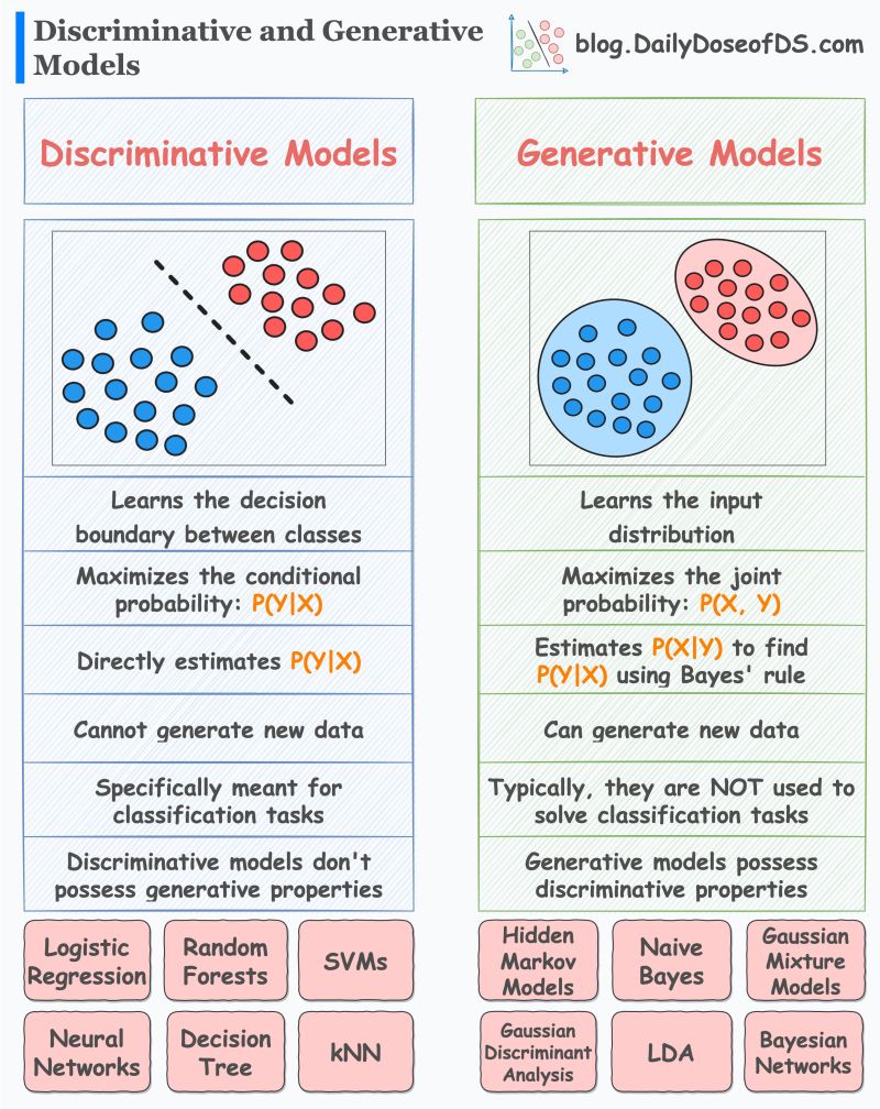
What are distance-weighted kNNs? What are the limitation of traditional kNNs?
- kNNs, by default, classify a new data point as follows:
- Count its class-wise “k” nearest neighbors
- Assign the data point to the class with the highest count
- As a result, during classification, the vicinity of a class is entirely ignored.
- Yet, this may be extremely important, especially when you have a class with few samples.
- Distance-weighted kNNs are a more robust alternative to traditional kNNs.
- As the name suggests, they consider the distance to the nearest neighbor during prediction.
- Thus, the closer a specific neighbor, the more will be its impact on the final prediction.
- Its effectiveness is evident from the image below (source).
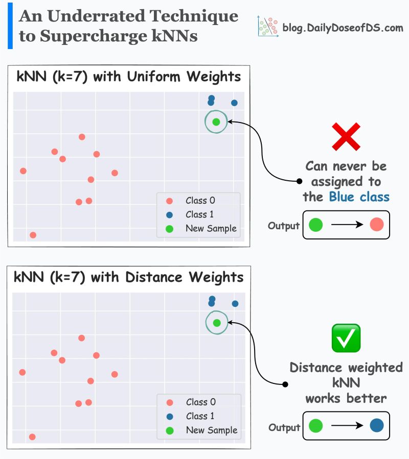
- Traditional kNN (with k=7) will never predict the blue class, while distance-weighted kNN is more robust in its prediction.
- Typically, a distance-weighted kNN works much better than a traditional kNN. And this makes intuitive sense as well.
- Yet, their utility may go unnoticed. This is because many frameworks like sklearn consider “uniform” weighting by default.
How does Kafka work as a Pub-Sub?
- Topics: Kafka divides its messages into categories called Topics. A topic is like a table in a database, and the messages are the rows in that table.
- Producers: Producers are applications that publish (or write) records to Kafka.
- Consumers: Consumers are the applications that subscribe to (read and process) data from Kafka topics.
- Brokers: A Kafka server is also called a broker; it is responsible for reliably storing data provided by the producers and making it available to the consumers.
- Records: A record is a message or an event that gets stored in Kafka.
- Message Flow:
- Each message that Kafka receives from a producer is associated with a topic.
- Consumers can subscribe to a topic to get notified when new messages are added to that topic.
- A topic can have multiple subscribers that read messages from it.
- In a Kafka cluster, a topic is identified by its name and must be unique.
- Messages in a topic can be read as often as needed -— unlike traditional messaging systems, messages are not deleted after consumption. Instead, Kafka retains messages for a configurable amount of time or until a storage size is exceeded. Kafka’s performance is effectively constant with respect to data size, so storing data for a long time is perfectly fine.
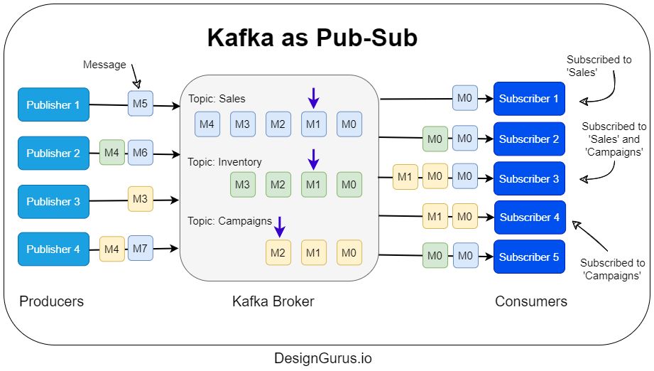
How do you swap two numbers without a temporary variable?
- Credits for this answer go to Prateek Chandra Jha.
- One of the most ingenious uses of the bitwise XOR operation is in swapping two numbers without using a temporary variable. This trick is often cited in computer science curriculum and coding interviews because of its clever exploitation of the properties of XOR.
- Properties of XOR used in this context:
- A XOR A = 0
- A XOR 0 = A
- A XOR B = B XOR A (Commutative)
- (A XOR B) XOR C = A XOR (B XOR C) (Associative)
- A XOR B XOR A = B
- Using the above properties, we can swap two numbers
aandbas follows:- a = a XOR b
- b = a XOR b which is equivalent to b = (a XOR b) XOR b = a XOR (b XOR b) = a XOR 0 = a
- a = a XOR b which is equivalent to a = (a XOR b) XOR a = b XOR (a XOR a) = b XOR 0 = b
- Real-world Example:
- Let’s say you’re working on a multiplayer card game. Each player has two cards in their hands, and there’s an option for players to exchange (swap) their cards instantly.
- In the game’s programming, each card has a unique number ID. To make the card exchange operation efficient, you don’t want to use extra memory (even if it’s small) to store temporary values. This is especially crucial if thousands of exchanges are happening in real-time.
- Here, the XOR swap becomes handy:
- Player A has card with ID
a. - Player B has card with ID
b.
- Player A has card with ID
- To swap them without using a temporary variable:
a = a XOR bb = a XOR ba = a XOR b
- After these operations, Player A will have the card with ID
b, and Player B will have the card with IDa. - It’s worth noting that in modern-day programming, compilers are highly optimized, and this trick might not offer a noticeable performance improvement. Moreover, readability and clarity of code are often more valued, so using a temporary variable for swapping is more common. However, the XOR swap remains a classic demonstration of a clever bit-level technique.
How would a compiler tackle swap operations in a program?
- Credits for this answer go to Prateek Chandra Jha.
- Modern compilers utilize a range of optimizations to produce efficient machine code. When it comes to swapping variables, compilers often employ strategies based on the specific context of the code and the target architecture.
- Using Registers: Modern processors have several registers, which are small storage areas directly on the CPU. When swapping two variables, a compiler might load one of the variables into a register, move the other variable to the original’s place, and then take the value from the register to place it in the second variable’s original position. This is essentially the classic temporary variable swap, but it’s done using fast CPU registers.
- Optimized XOR Swap: A modern compiler might recognize this pattern and potentially optimize it further. However, this doesn’t necessarily mean that the XOR trick will be used in the generated machine code. The compiler could decide that a register-based swap (as mentioned above) is faster and transform the XOR-based swap into a register-based one.
- Elimination of Swap: In certain contexts, the compiler might determine that the swap operation is redundant and can be safely eliminated without affecting the program’s behavior. For instance, if the variables are swapped back to their original values later in the code and there’s no use of the swapped values in between, then the compiler might just eliminate the swaps entirely.
- Using SIMD (Single Instruction, Multiple Data) Instructions: On architectures that support SIMD, multiple data elements can be processed in parallel. In certain contexts, swapping operations can be optimized using SIMD instructions.
- Inlining and Other Optimizations: If the swapping operation is part of a small function that gets called multiple times, the compiler might inline the function (replace the function call with the function’s content) to eliminate the overhead of the function call. Once inlined, the swapping operation can be further optimized in the context of the calling function.
- Real-world Example:
- Imagine a graphics program that’s performing operations on pairs of pixel values. Let’s say there’s a piece of code that frequently swaps these pixel values:
void swap(int *a, int *b) { int temp = *a; *a = *b; *b = temp; } - In a loop that calls this function thousands of times, a modern compiler might inline the swap function right into the loop to avoid the overhead of the function calls. Furthermore, if the loop swaps the values back to their original state later on without any significant computation in between, the compiler might even eliminate these swap operations altogether, judging them as redundant.
- Imagine a graphics program that’s performing operations on pairs of pixel values. Let’s say there’s a piece of code that frequently swaps these pixel values:
How are XOR Filters used? What if you require better performance than Bloom filters?
- Credits for this answer go to Dev Agarwal.
- Bloom Filters trade-off latency for performance (in terms of false positives). But can we do better to minimize these false positives? Indeed, we can! Introducing a new player in the data structure arena: the XOR Filter.
- As the name suggests, XOR Filters leverage XOR (exclusive OR) operations to encode the presence of elements. This advanced technique comes with a more intricate setup involving auxiliary arrays and values, but it offers an intriguing advantage – better accuracy as shown in the figure below.
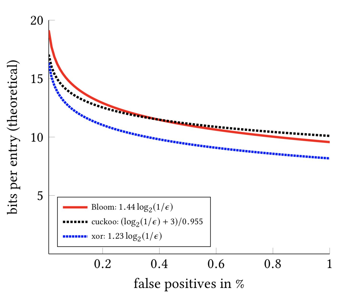
- Let’s break the process into steps to understand a bit more:
- Hash each word to produce an array of hashes.
- XOR the hashes together to form a single value.
- Store this XOR value. For our example, let’s say we hash “apple” to hash(apple) = 3, “banana” to hash(banana) = 7, and “cherry” to hash(cherry) = 4. The XOR of these hash values would be 3 XOR 7 XOR 4 = 4.
- Now, when checking for the presence of “cherry,” we hash it to hash(cherry) = 4 and XOR it with the stored XOR value of 4. If the result is 0, “cherry” is likely in the set.
- While this example simplifies the process, XOR filters offer more accurate set membership testing and can handle more elements before becoming prone to false positives compared to Bloom filters. However, implementing XOR filters can be more complex and might require more memory than Bloom filters.
- As a detailed example:
- Let’s say we’re building an XOR filter to check if a given number is present in a set of integers. We’ll use a simplified version of the algorithm, and for clarity, here’s an end-to-end example:
- Step 1: Hashing
- We have a set of integers: 7, 15, and 23.
- We apply a hash function to each integer to generate hash values: - Hash(7) = 2 - Hash(15) = 1 - Hash(23) = 3
- Step 2: Creating XOR Values
- We create XOR values by combining the hash values using bitwise XOR.
- XOR Value = Hash(7) XOR Hash(15) XOR Hash(23) = 2 XOR 1 XOR 3 = 0.
- Step 3: Storing the XOR Value
- We store the XOR value (0) for the set of integers (7, 15, 23).
- Step 4: Checking Membership
- Now, let’s check if a new number, 10, is in the set.
- We hash 10: Hash(10) = 2.
- We XOR Hash(10) with the stored XOR value: 2 XOR 0 = 2.
- Step 5: Determining Membership
- If the result of the XOR operation is 0, then it’s likely that the number is in the set. In this case, 10 is not in the set since 2 XOR 0 is not 0.
- Real-World Analogy:
- Think of the XOR value as a “fingerprint” of the set. It’s derived from the hash values of the elements and captures their combined presence. When you want to check if a new number is in the set, you hash the new number, XOR it with the stored XOR value, and see if the result matches 0. If it does, there’s a high chance the number is in the set; if not, it’s likely not in the set.
- This XOR filtering approach boasts a higher accuracy rate than Bloom filters when it comes to reducing false positives. Nevertheless, it’s important to note that constructing and maintaining XOR filters can demand more memory and computational resources compared to their Bloom counterparts.
- Compared to Bloom or Cuckoo filters, XOR filters are immutable. They are meant to be built once and used many times, unlike Bloom or Cuckoo filters where elements can be added dynamically. It makes XOR filters unfit for many “online” use-cases.
What are indexing techniques for NoSQL databases?
- Credits for this answer go to Prateek Chandra Jha.
- NoSQL databases (usually) run faster than SQL databases, thanks to their ease of scalability and the intelligent indexing techniques they use under-the-hood.
- In NoSQL databases, indexing techniques vary based on the type of NoSQL database (document-based, key-value, columnar, or graph). Regardless of the type, the goal of indexing is to improve data retrieval performance. Let’s dive into some common indexing techniques across different NoSQL database types:
- B-Tree Indexing:
- Used by many NoSQL databases, including some configurations of MongoDB.
- Like in relational databases, B-trees can quickly locate data based on the indexed key. They are particularly useful for range queries.
- Hash Indexing:
- Common in key-value stores like Redis.
- Given a key, the database applies a hash function to find the location of the corresponding value.
- It’s very efficient for point queries (where you’re looking up a single key-value pair) but not for range queries.
- Compound Indexing:
- Used in document stores like MongoDB.
- Allows for creating indexes on multiple fields. This is particularly useful when queries need to filter or sort by multiple fields.
- Geospatial Indexing:
- Many NoSQL databases like MongoDB and Elasticsearch support this.
- Used to index data based on geographic location. For instance, you could use a geospatial index to quickly retrieve all restaurants within a 5-mile radius of a specific point.
- Bitmap Indexing:
- Often used in column-family stores like HBase or Cassandra.
- Efficient for scenarios where the indexed column has a low cardinality (i.e., a limited number of unique values).
- Uses a bitmap for each unique value and sets bits for rows that have that value.
- Inverted Indexing:
- Common in full-text search databases like Elasticsearch.
- Instead of mapping documents to keywords (like a traditional index), it maps keywords to the list of documents that contain them. This is essential for efficient full-text search operations.
- Secondary Indexing:
- Provides a way to query data on non-primary key columns.
- Used in databases like Cassandra where the primary mode of access is through the primary key. A secondary index allows for efficient querying on other columns.
- Edge Indexing:
- Used in graph databases like Neo4j.
- Helps in efficiently traversing relationships (edges) in the graph.
- Prefix Indexing:
- Used in databases like Redis.
- Helps in efficiently querying keys with a common prefix.
- Sparse Indexing:
- Particularly useful in databases like MongoDB for collections where only a subset of documents contains the indexed field.
- Instead of having an entry for each document in the collection, the sparse index only includes entries for documents that have the indexed field.
- B-Tree Indexing:
- While these are some of the common indexing techniques, NoSQL databases often combine and customize these techniques based on their architecture and use-case specifics.
Does DPO for LLM alignment use the Bradley-Terry model? If so, how?
-
The Direct Preference Optimization (DPO) method for aligning Large Language Models (LLMs) does use the Bradley-Terry model. Here’s a detailed explanation of how the Bradley-Terry model is used in DPO for LLM alignment:
- Overview of the Bradley-Terry Model:
- The Bradley-Terry model is a probability model used for pairwise comparisons. It assigns a score to each item (in this context, model outputs), and the probability that one item is preferred over another is a function of their respective scores. Formally, if item \(i\) has a score \(s_i\) and item \(j\) has a score \(s_j\), the probability \(P(i \text{ is preferred over } j)\) is given by:
- Application in DPO for LLM Alignment:
- Data Collection:
- Human evaluators provide pairwise comparisons of model outputs. For example, given two responses from the LLM, the evaluator indicates which one is better according to specific criteria (e.g., relevance, coherence, correctness).
- Modeling Preferences:
- The outputs of the LLM are treated as items in the Bradley-Terry model. Each output has an associated score reflecting its quality or alignment with human preferences.
- Score Estimation:
- The scores \(s_i\) for each output are estimated using the observed preferences. If output \(i\) is preferred over output \(j\) in several comparisons, \(s_i\) will be higher than \(s_j\). The scores are typically estimated using maximum likelihood estimation (MLE) or other optimization techniques suited for the Bradley-Terry model.
- Optimization:
- Once the scores are estimated, the LLM is fine-tuned to maximize the likelihood of generating outputs with higher scores. The objective is to adjust the model parameters so that the outputs align better with human preferences as captured by the Bradley-Terry model scores.
- Data Collection:
- Detailed Steps in DPO:
- Generate Outputs:
- Generate multiple outputs for a given prompt using the LLM.
- Pairwise Comparisons:
- Collect human feedback by asking evaluators to compare pairs of outputs and indicate which one is better.
- Fit Bradley-Terry Model:
- Use the collected pairwise comparisons to fit the Bradley-Terry model and estimate the scores for each output.
- Update LLM:
- Fine-tune the LLM using the estimated scores. The objective is to adjust the model parameters such that the likelihood of producing higher-scored (preferred) outputs is maximized. This step often involves gradient-based optimization techniques where the loss function incorporates the Bradley-Terry model probabilities. - By iteratively performing these steps, the LLM can be aligned more closely with human preferences, producing outputs that are more likely to be preferred by human evaluators.
- Generate Outputs:
- Summary:
- The Bradley-Terry model plays a crucial role in the Direct Preference Optimization method by providing a statistical framework for modeling and estimating the preferences of different model outputs. This, in turn, guides the fine-tuning of the LLM to align its outputs with human preferences effectively.
Are k-Nearest Neighbors and k-means clustering parametric?
- The terms “parametric” and “non-parametric” refer to whether a method makes strong assumptions about the form of the underlying distribution of the data. Both k-NN and k-means clustering are non-parametric methods because they do not assume a specific form for the underlying data distribution and rely heavily on the data itself rather than predefined parameters.Let’s examine k-Nearest Neighbors (k-NN) and k-means clustering in this context.
k-Nearest Neighbors (k-NN)
- k-NN is considered a non-parametric method. This is because k-NN does not make any assumptions about the underlying distribution of the data. Instead, it relies on the distance between data points to make predictions or classifications. The model is defined by the training data itself rather than parameters that summarize the data.
k-means Clustering
- k-means clustering is also considered a non-parametric method. While k-means does make an assumption about the number of clusters (k), it does not make strong assumptions about the form of the data distribution within those clusters. Instead, it iteratively partitions the data into k clusters based on distance measures. The means of the clusters are updated iteratively based on the current assignment of points to clusters, but this process does not depend on a fixed set of parameters that describe the overall data distribution.
How are code LLMs trained with the “fill-in-the-middle” pre-training task?
- The implementation of “Fill-in-the-middle” (FIM) as a pre-training task in the loss function involves designing the training process to predict the missing middle section of a code sequence given the surrounding context (prefix and suffix). Here’s a detailed breakdown of how this can be integrated into the loss function:
Implementation of FIM in the Loss Function
- Data Preparation:
- Segmenting Code: For each code snippet in the training data, divide the sequence into three parts: the prefix (beginning of the code), the suffix (end of the code), and the middle section, which is to be predicted.
- Masking the Middle: The middle section is replaced with a special mask token that indicates to the model that this part needs to be generated.
- Model Architecture:
- Input Representation: Concatenate the prefix and suffix, inserting the special mask token where the middle section should be.
- Contextual Encoding: The model processes the concatenated input to generate contextual embeddings for the prefix, mask token, and suffix.
- Prediction Mechanism:
- Decoder Input: The model’s decoder (or the autoregressive part of the transformer) is provided with the context from the encoder and the mask token to generate the middle section.
- Sequence Generation: The model generates tokens sequentially for the middle section, leveraging the contextual information from both the prefix and suffix.
- Loss Function Design:
- Cross-Entropy Loss: The primary loss function used is typically the cross-entropy loss, which measures the difference between the predicted tokens and the actual tokens in the middle section.
- Masked Tokens Loss Calculation: Only the positions corresponding to the middle section are considered for the loss calculation. The loss is computed by comparing the predicted tokens with the actual tokens in the masked middle section.
Detailed Steps for Loss Calculation
- Token-Level Prediction:
- For each token position in the middle section, the model outputs a probability distribution over the vocabulary.
- Let \(y_{true}\) be the actual token and \(y_{pred}\) be the predicted probability distribution for a given position in the middle section.
- Cross-Entropy Loss for Each Token:
- The cross-entropy loss for a single token position \(i\) is calculated as: \(\text{Loss}_i = -\log P(y_{true,i} | \text{context})\) where \(P(y_{true,i} | \text{context})\) is the predicted probability of the true token \(y_{true,i}\) given the context (prefix and suffix).
- Aggregate Loss:
- The total loss for a single training example is the sum of the cross-entropy losses for all token positions in the middle section: \(\text{Total Loss} = \sum_{i \in \text{middle}} \text{Loss}_i\)
- Batch Loss:
- The loss is averaged over all training examples in the batch to obtain the final loss used for backpropagation: \(\text{Batch Loss} = \frac{1}{N} \sum_{j=1}^N \text{Total Loss}_j\) where \(N\) is the number of training examples in the batch and \(\text{Total Loss}_j\) is the total loss for the \(j\)-th example.
Practical Example
- Assume a code snippet is split as follows:
- Prefix:
def add_numbers(a, b): - Suffix:
return a + b - Middle:
[body placeholder]
- Prefix:
- The input to the model during training would look like:
def add_numbers(a, b): [MASK] return result
- The model needs to predict the masked middle part, which might be an indentation followed by the main logic, such as:
result = a + b - During training, the model is penalized for the difference between its predicted tokens for the middle section and the actual tokens.
- By incorporating this FIM objective into the loss function, the model learns to generate code that coherently fits within the given context, improving its ability to handle tasks where code needs to be inserted or completed in the middle of existing code blocks.
For a RAG pipeline aimed at a code generation use-case, what is typically chunked and retrieved for the RAG aspect?
- In a RAG (Retrieval-Augmented Generation) pipeline for code generation, the chunks that are typically retrieved and used can vary depending on the specific use-case and the granularity required. However, the most common chunks include:
Code Snippets
- Code Segments:
- Short, reusable pieces of code that solve specific problems or perform certain functions. These can be function definitions, loops, conditionals, or smaller logic blocks.
- Example:
  def add_numbers(a, b):
      return a + b
Code Templates
- Code Patterns:
- More extensive templates that provide a skeleton or structure for common coding tasks. These templates can include boilerplate code for setting up frameworks, classes, or entire scripts.
- Example:
  class MyClass:
      def __init__(self, param):
          self.param = param

      def method(self):
          pass
Documentation and Comments
- API Documentation:
- Relevant parts of documentation that describe how to use specific functions, classes, or libraries. This can include usage examples, parameter descriptions, and return values.
- Example:
```plaintext
Function: add_numbers(a, b)
- Adds two numbers and returns the result.
- Parameters:
- a: int or float, the first number
- b: int or float, the second number
- Returns:
- int or float, the sum of a and b ```
Stack Overflow and Forum Posts
Q&A Snippets:
- Excerpts from question-and-answer sites like Stack Overflow, where similar problems have been discussed and solved. These snippets often include practical solutions and discussions about best practices.
Example:
Q: How can I sum two numbers in Python?
A: You can use the simple addition operator:
```python
result = a + b
### 5. Code Comments and Explanations
**Inline Comments:**
- Comments within code that explain the purpose and logic of specific lines or blocks. These are crucial for understanding and modifying the code.

**Example:**
```python
def add_numbers(a, b):
    # This function takes two numbers and returns their sum
    return a + b
Configuration and Setup Files
- Config Files:
- Examples of configuration files (e.g., JSON, YAML) and setup scripts that are commonly used in specific environments or projects.
- Example:
  {
    "setting1": "value1",
    "setting2": "value2"
  }
Chunking Strategy
-
The chunking strategy typically involves:
- Granularity:
- Splitting the code and associated text into logical and functional units that can be independently retrieved and recombined.
- Context Preservation:
- Ensuring that each chunk retains enough context to be meaningful when retrieved. This might involve including preceding and following lines of code or associated documentation.
- Indexing:
- Indexing these chunks using a search engine (e.g., Elasticsearch) or an approximate nearest neighbor search tool (e.g., FAISS) to facilitate fast and accurate retrieval.
- Granularity:
Example RAG Workflow
- Query Input:
- A user inputs a query or a partial code snippet.
- Retrieval:
- The system uses the retrieval model to fetch relevant code snippets, templates, documentation, and comments from the indexed chunks.
- Generation:
- The generative model takes the retrieved chunks and the user’s input to generate a complete and contextually appropriate code snippet.
- Output:
- The final code generation is presented to the user, combining the retrieved information and newly generated content.
- By chunking and retrieving these various types of information, the RAG pipeline can provide highly relevant and context-aware code generation assistance.
For a RAG pipeline aimed at a SQL generation use-case, what is typically chunked and retrieved for the RAG aspect?
- For a RAG (Retrieval-Augmented Generation) pipeline aimed at SQL generation, the chunks that are typically retrieved can include a variety of SQL-related components. These chunks help in understanding the context, structure, and specifics of SQL queries. Here are the primary types of chunks:
SQL Queries
- Common Queries:
- Frequently used SQL queries that cover standard operations such as SELECT, INSERT, UPDATE, DELETE, JOIN, and aggregate functions.
- Example:
SELECT name, age FROM users WHERE age > 30;
Query Templates
- Parameterized Templates:
- Reusable query structures that can be easily adapted to different tables and columns. These templates often include placeholders for dynamic content.
- Example:
SELECT {columns} FROM {table} WHERE {condition};
Database Schema Information
- Table Definitions:
- Definitions of database schemas, including table structures, column names, data types, constraints, and relationships between tables.
- Example:
  Table: users
  Columns: id (INT, PRIMARY KEY), name (VARCHAR), age (INT), email (VARCHAR)
SQL Functions and Procedures
- Stored Procedures:
- Examples of stored procedures and functions that perform specific tasks within the database. These can be particularly useful for complex operations.
- Example:
  CREATE PROCEDURE GetUserAge (IN userId INT)
  BEGIN
      SELECT age FROM users WHERE id = userId;
  END;
SQL Documentation and Best Practices
- Guidelines:
- Documentation snippets and best practices for writing efficient and secure SQL queries. This includes indexing strategies, query optimization tips, and security considerations.
- Example:
To optimize SELECT queries, ensure that frequently queried columns are indexed.
Query Optimization Techniques
- Performance Tips:
- Explanations and examples of how to optimize SQL queries for better performance, including the use of indexes, query restructuring, and avoiding common pitfalls.
- Example:
Use INNER JOIN instead of subqueries for better performance.
Example Use-Cases and Query Patterns
- Use-Case Specific Queries:
- Example queries tailored to specific use-cases such as reporting, data analysis, user management, etc. These provide practical examples that can be adapted to similar scenarios.
- Example:
SELECT COUNT(*) FROM orders WHERE order_date BETWEEN '2023-01-01' AND '2023-12-31';
Chunking Strategy
-
The chunking strategy for SQL generation typically involves:
-
Granularity: Breaking down the SQL queries and related information into logical units that can be retrieved and recombined. This might include individual clauses (e.g., SELECT, FROM, WHERE), complete queries, and schema definitions.
-
Context Preservation: Ensuring that each chunk retains enough context to be meaningful. For instance, a WHERE clause chunk should include references to the table and columns it applies to.
-
Indexing: Indexing these chunks using a search engine (e.g., Elasticsearch) or an approximate nearest neighbor search tool (e.g., FAISS) to facilitate fast and accurate retrieval.
-
Example RAG Workflow for SQL Generation
- Query Input:
- A user inputs a natural language query or a partial SQL statement.
- Retrieval:
- The system uses the retrieval model to fetch relevant SQL queries, templates, schema information, and documentation from the indexed chunks.
- Generation:
- The generative model takes the retrieved chunks and the user’s input to generate a complete and contextually appropriate SQL query.
- Output:
- The final SQL query is presented to the user, combining the retrieved information and newly generated content.
- By chunking and retrieving these various types of SQL-related information, the RAG pipeline can provide highly relevant and context-aware SQL query generation assistance, helping users to write efficient and accurate queries tailored to their specific needs.
How is logistic regression a linear model if the sigmoid function is non-linear?
- Logistic regression is considered a linear model, though it incorporates a non-linear function. The linearity in logistic regression refers to the linear relationship between the input features and the log-odds of the outcome, not necessarily the direct relationship between the features and the predicted probability.
- In logistic regression, the model predicts the probability of an outcome by first calculating a linear combination of the input features, expressed as:
- This linear combination \(z\) is then passed through a sigmoid function (also known as a logistic function):
- The sigmoid function maps \(z\) to a value between 0 and 1, representing the probability of the outcome. While the sigmoid function is non-linear, logistic regression is still considered a linear model because the key relationship in the model—the relationship between the input features and the log-odds (the logarithm of the odds) of the outcome—is linear.
- In summary, logistic regression is a linear model with respect to the log-odds, but it uses the non-linear sigmoid function to produce probabilities.
How much memory is needed to serve a Large Language Model (LLM)?
- Here’s the math behind deploying a model with size \(P\). Here’s a formula that can help you estimate the GPU memory required for serving an LLM:
- where:
- \(M\) is the GPU memory in Gigabytes.
- \(P\) is the number of parameters in the model.
- \(4B\) represents the 4 bytes used per parameter.
- \(Q\) is the number of bits for loading the model.
- 1.2 accounts for a 20% overhead.
- This overhead isn’t just a buffer - it’s crucial for additional memory used during inference, such as storing activations (intermediate results) of the model. Along with the model, the input data (i.e., the batch) is also stored in GPU VRAM during inference. Thus, the model’s weights, input batch, and its intermediate activations are all need to fit into GPU VRAM for inference.
What is Consistent Hashing in Distributed Systems?
Overview
- Consistent hashing is a key algorithm used in distributed systems to distribute data across multiple nodes in a way that minimizes data reorganization when nodes are added or removed. It is particularly important in systems where nodes can dynamically join or leave, such as in distributed databases, caching systems, and peer-to-peer networks.
Problem with Traditional Hashing
- In traditional hashing, keys are mapped to a fixed set of buckets (nodes). For instance, if a hash function maps keys to buckets using modulo operation (e.g.,
hash(key) % N, whereNis the number of nodes), adding or removing a node requires redistributing all keys across the new set of nodes. This leads to a large amount of data movement, which is inefficient.
How Consistent Hashing Works
- Consistent hashing addresses this problem by mapping both the data keys and the nodes to a virtual circular hash space, often visualized as a ring.
- Hash Space and Ring:
- The hash space is usually represented as a circle (a “ring”) where the hash function outputs values that can be thought of as points on this ring.
- Nodes and keys are assigned positions on this ring using the same hash function.
- Assigning Keys to Nodes:
- Each key is mapped to the closest node in the clockwise direction on the ring. This means that each node is responsible for the range of keys between it and the next node in the clockwise direction.
- Adding or Removing Nodes:
- Adding a Node: The new node will only take responsibility for a portion of the keys from the existing node that was previously responsible for that range, minimizing the data movement.
- Removing a Node: Only the nodes immediately adjacent to the removed node will take over its keys, again minimizing disruption.
Virtual Nodes (vNodes)
- To prevent uneven distribution of keys, consistent hashing often uses a technique called virtual nodes (vNodes). Each physical node is assigned multiple virtual nodes, which are spread across the hash space. This increases the likelihood of an even distribution of keys, even if the physical nodes themselves are unevenly distributed or vary in number.
Advantages
- Scalability: The system can easily scale by adding or removing nodes with minimal data movement.
- Load Balancing: Virtual nodes help in evenly distributing the load across all physical nodes.
- Fault Tolerance: If a node fails, only the nodes adjacent to it in the hash ring are affected, making the system more resilient.
Use Cases
- Distributed Caching Systems: Systems like Amazon DynamoDB and Apache Cassandra use consistent hashing to distribute data across multiple nodes in a cluster.
- Load Balancers: Load balancers use consistent hashing to ensure that requests from the same client are directed to the same server, improving cache hit rates.
- Content Delivery Networks (CDNs): CDNs use consistent hashing to distribute content across multiple edge servers.
Conclusion
- Consistent hashing is a powerful tool in distributed systems that provides a scalable and efficient way to manage data across dynamic and distributed environments. By minimizing the amount of data that needs to be moved when changes occur, it ensures that the system remains performant and resilient even as it scales.
What are some load balancing algorithms in distributed systems?
- Load balancing in distributed systems is a critical technique used to distribute workload across multiple computing resources (such as servers, CPUs, or network links) to ensure no single resource is overwhelmed. The goal is to optimize resource use, maximize throughput, minimize response time, and avoid overload. Below are some common load balancing algorithms used in distributed systems:
Round Robin
- Mechanism: Requests are distributed sequentially among all available resources in a circular order.
- Use Case: Simple and effective when all servers have similar capacity.
- Pros: Easy to implement and understand.
- Cons: Doesn’t consider the current load on each resource, which can lead to inefficient utilization if servers have different capacities or are unevenly loaded.
Weighted Round Robin
- Mechanism: Similar to Round Robin but assigns a weight to each server based on its capacity or other criteria. Servers with higher weights receive more requests.
- Use Case: Useful when the resources have varying capacities.
- Pros: Takes into account the differences in server capacity.
- Cons: Still doesn’t consider real-time load on servers.
Least Connections
- Mechanism: Directs traffic to the server with the fewest active connections.
- Use Case: Suitable for environments where connection durations vary significantly.
- Pros: Balances load more effectively in environments with variable connection lengths.
- Cons: May not be efficient if the time required to process requests varies significantly.
Weighted Least Connections
- Mechanism: An extension of Least Connections where servers are also assigned weights. Servers with more capacity (higher weight) will receive more connections but still prefer those with fewer active connections.
- Use Case: Useful when servers have different capacities and connection durations vary.
- Pros: More nuanced distribution than simple Least Connections.
- Cons: More complex to implement and requires proper configuration of weights.
Least Response Time
- Mechanism: Directs traffic to the server with the lowest average response time.
- Use Case: Effective in environments where response time is a critical metric.
- Pros: Ensures requests are directed to the most responsive servers.
- Cons: Requires real-time monitoring and may not adapt quickly to sudden changes in server load.
IP Hashing
- Mechanism: Uses the client’s IP address to compute a hash, which then determines which server will handle the request.
- Use Case: Ensures the same client is consistently directed to the same server (session persistence).
- Pros: Simple and effective for session persistence.
- Cons: Can lead to uneven distribution if there is a skew in client IP distribution.
Consistent Hashing
- Mechanism: Distributes requests based on a hash of the request, such as the client’s IP address or a specific resource identifier. Servers are also hashed, and requests are routed to the closest server in the hash ring.
- Use Case: Highly effective in distributed systems where nodes can join or leave dynamically (e.g., caching systems like Memcached).
- Pros: Minimizes the number of keys that need to be remapped when nodes are added or removed.
- Cons: More complex to implement than simple hashing.
Randomized Load Balancing
- Mechanism: Requests are assigned randomly to any available resource.
- Use Case: Suitable for large-scale systems with many resources where uniform distribution is likely over time.
- Pros: Extremely simple to implement.
- Cons: May result in uneven distribution in the short term.
Centralized Load Balancing
- Mechanism: A central node monitors and manages the load on all resources and assigns incoming requests based on this global knowledge.
- Use Case: Systems where a central authority can optimize global performance.
- Pros: Can achieve optimal load distribution if the central node has accurate and up-to-date information.
- Cons: Single point of failure and potential bottleneck.
Distributed Load Balancing
- Mechanism: Each node independently decides where to forward requests based on local load information.
- Use Case: Highly distributed systems where central coordination is impractical.
- Pros: Scalable and fault-tolerant.
- Cons: Can be less efficient due to lack of global information.
Dynamic Load Balancing
- Mechanism: Load balancing decisions are made dynamically based on real-time metrics such as server load, response time, or other performance indicators.
- Use Case: Environments with rapidly changing workloads.
- Pros: Adaptable to changing conditions, ensuring efficient load distribution.
- Cons: Complexity in implementation and the need for continuous monitoring.
Agent-Based Load Balancing
- Mechanism: Agents on each node autonomously manage and distribute load by communicating with other agents, making local decisions based on global information.
- Use Case: Complex, large-scale distributed systems where decentralized decision-making is preferred.
- Pros: High fault tolerance and adaptability.
-
Cons: Complexity and overhead in maintaining communication between agents.
- Each algorithm has its strengths and weaknesses, and the choice of algorithm depends on the specific requirements of the distributed system, such as the nature of the workload, the capacity of the resources, and the performance goals. In many systems, a combination of these algorithms may be used to achieve the best performance.
Why is Flash attention needed, and how does it work?
- Flash Attention is a technique designed to improve the efficiency and performance of the attention mechanism in transformers, which are a type of neural network architecture widely used in natural language processing (NLP) and other areas. Flash Attention is motivated by the need to address the inefficiencies and scalability issues inherent in the traditional implementation of attention mechanisms, especially as the size of models and datasets continues to grow.
- Flash Attention addresses key limitations of traditional attention mechanisms by optimizing memory usage and computational efficiency. By implementing more memory-efficient algorithms, tiling strategies, kernel fusion, and other optimizations, Flash Attention enables transformers to handle longer sequences and larger models, making it a critical advancement for scaling up NLP models and improving their deployment in real-world applications.
Why is Flash Attention Needed?
-
Computational Complexity: Traditional attention mechanisms have a computational complexity of (O(N^2)) where (N) is the sequence length. This quadratic scaling can become a significant bottleneck as the sequence length increases, making it computationally expensive and memory-intensive. For large models or long sequences, this can be a major limitation.
-
Memory Usage: The standard attention mechanism requires storing large attention matrices, which scale with the square of the sequence length. This leads to high memory consumption, which can quickly exhaust the available memory on GPUs, limiting the size of sequences that can be processed.
-
Performance Bottlenecks: As the sequence length increases, the time taken to compute the attention grows, leading to latency issues. This can make real-time or low-latency applications challenging when using large transformers.
-
Scalability: To deploy transformers in production or to train very large models efficiently, scalability is essential. The traditional attention mechanism’s limitations in both computation and memory make scaling up models and handling long sequences more difficult.
How Does Flash Attention Work?
-
Flash Attention is a more efficient implementation of the attention mechanism, focusing on reducing memory usage and computational overhead. It achieves this through a few key innovations:
-
Memory-Efficient Algorithm: Flash Attention avoids the need to materialize the full attention matrix, which is typically done in traditional implementations. Instead, it computes attention scores and performs the softmax operation in a more memory-efficient manner. This approach reduces memory bandwidth usage and helps in fitting longer sequences into the available GPU memory.
-
Tiling and Partitioning: Flash Attention divides the sequence into smaller tiles or blocks and processes them sequentially. This tiling strategy allows the attention computation to be performed on smaller chunks of data, reducing the peak memory usage. By only keeping the necessary parts of the sequence in memory at any given time, Flash Attention can handle longer sequences more efficiently.
-
Kernel Fusion and Optimization: The implementation of Flash Attention often uses optimized custom CUDA kernels to perform multiple operations in a single pass. This reduces the number of memory read and write operations, increasing throughput and reducing latency. Kernel fusion combines operations like matrix multiplication, softmax, and scaling into a single kernel, which minimizes overhead.
-
Low-Rank Approximations: In some variants of Flash Attention, low-rank approximations of the attention matrix are used. This approximation reduces the dimensionality of the problem, making it computationally cheaper while still capturing the most important information in the attention scores.
-
On-the-Fly Computation: Instead of storing large intermediate matrices, Flash Attention computes values on the fly as needed. This reduces memory pressure and allows for more efficient use of cache memory.
-
Benefits of Flash Attention
-
Reduced Memory Footprint: By avoiding the need to store full attention matrices and using a tiled computation approach, Flash Attention significantly reduces the memory required for attention computation.
-
Improved Speed and Efficiency: Flash Attention’s optimized computation and reduced memory usage lead to faster execution, making it suitable for real-time applications and enabling larger models to be trained and deployed.
-
Scalability: The reduced computational and memory demands make Flash Attention more scalable, allowing it to handle longer sequences and larger models without running into the same bottlenecks as traditional attention mechanisms.
-
Better Utilization of Hardware Resources: By leveraging GPU memory more efficiently and reducing memory bandwidth requirements, Flash Attention makes better use of available hardware, potentially lowering infrastructure costs and energy consumption.
What is Continuous and dynamic batching?
- Continuous and dynamic batching are concepts related to optimizing the processing of tasks or data in systems, particularly in the context of machine learning, data processing, and distributed computing. These approaches help to improve the efficiency and throughput of systems by adjusting how data is grouped and processed based on current conditions and demands. Let’s explore each concept in detail:
Continuous Batching
- Continuous batching refers to a method where incoming data or tasks are continuously accumulated into batches over time until certain conditions are met. This approach is commonly used in scenarios where tasks or data arrive at unpredictable rates, and it is beneficial to process them in groups rather than individually to improve efficiency.
- Both continuous and dynamic batching are techniques that help manage how tasks and data are processed in systems. Continuous batching accumulates tasks into batches over time, while dynamic batching adjusts batch sizes and timing based on real-time system conditions. These methods are essential for optimizing performance, reducing latency, and ensuring efficient use of computational resources in various applications, including machine learning, data processing, and real-time analytics.
Key Characteristics of Continuous Batching
- Batch Formation: Data or tasks are accumulated over a time window or until a batch size threshold is reached.
- Efficiency: By processing data in batches, continuous batching can reduce the overhead associated with task switching, communication, and processing, leading to more efficient use of resources.
- Latency Considerations: While continuous batching can improve throughput, it may introduce some latency since data waits to be accumulated into a batch before being processed.
- Adaptability: Systems can adjust the batch size or time window dynamically based on current load or system conditions, allowing for flexibility in managing varying input rates.
Examples of Continuous Batching
- Stream Processing: In real-time data analytics, continuous batching can be used to group incoming data streams into micro-batches for processing, allowing for near-real-time analysis while maintaining efficiency.
- Machine Learning Training: In machine learning, especially with neural networks, training data is often processed in batches. Continuous batching can help accumulate training examples until a certain batch size is reached, then process them together for gradient updates.
Dynamic Batching
Dynamic batching is a more adaptive and intelligent approach where the system dynamically decides how to batch incoming tasks or data based on the current state of the system, such as load, available resources, and input rate. This method aims to optimize both latency and throughput by adjusting batch sizes and processing schedules in real-time.
Key Characteristics of Dynamic Batching
- Real-Time Adjustment: Unlike fixed or static batching, dynamic batching changes the size of the batches and how frequently they are processed based on real-time feedback.
- Resource Optimization: By adapting to the current state of system resources and load, dynamic batching can optimize resource utilization, balancing between maximizing throughput and minimizing latency.
- Predictive and Reactive: Dynamic batching can be both predictive (anticipating future load based on trends) and reactive (responding to current load and resource availability).
- Complexity: Implementing dynamic batching is more complex as it requires monitoring and decision-making algorithms to determine the optimal batch size and timing.
Examples of Dynamic Batching
- Online Inference in Machine Learning: When serving machine learning models for real-time predictions, requests may come in bursts. Dynamic batching can group requests into batches based on current load, optimizing GPU/TPU utilization and reducing waiting time for predictions.
- Distributed Computing Systems: In distributed data processing frameworks (e.g., Apache Spark), dynamic batching can adjust the task sizes sent to different nodes based on current processing speed and network conditions to optimize job completion time.
Comparison and Use Cases
- Continuous Batching is more about consistently accumulating data into batches for processing, which is effective for steady workloads or when batch processing is inherently more efficient. It’s typically used in applications where some latency is acceptable, and throughput is a higher priority.
- Dynamic Batching goes a step further by incorporating real-time adjustments to batch sizes and processing schedules, which is crucial in environments with fluctuating workloads and varying system states. It is particularly useful in scenarios where both latency and throughput need to be optimized, such as online inference, real-time analytics, or cloud-based services.
How does ColBERT carry out late interaction?
- ColBERT (Contextualized Late Interaction over BERT) is a neural retrieval model that optimizes the trade-off between efficiency and effectiveness in information retrieval tasks. The term “Late Interaction” refers to the way ColBERT delays the interaction between the query and document representations until the final stages of the retrieval process, rather than performing it during the encoding phase.
- Here’s a breakdown of how ColBERT carries out Late Interaction.
Independent Encoding of Queries and Documents
- BERT-based Encoding: ColBERT uses BERT (Bidirectional Encoder Representations from Transformers) to independently encode queries and documents into vectors.
- Each query is tokenized and fed through BERT to generate a set of token embeddings.
- Similarly, each document is tokenized and fed through BERT to generate a set of token embeddings.
- The key difference here from other retrieval models (like dense retrieval) is that ColBERT avoids encoding the interaction between the query and document at this stage. The two are processed separately to avoid early interaction (i.e., before retrieval), which is computationally expensive.
Maxsim Scoring (Late Interaction Stage)
- Once both the query and document are encoded into vectors, the Late Interaction occurs during the scoring phase.
- Specifically, ColBERT calculates the cosine similarity (or dot product) between each token embedding from the query and each token embedding from the document.
- The next step is the Maxsim operation, where for each query token, ColBERT identifies the maximum similarity score across all document tokens. This operation allows the model to focus on the most relevant parts of the document for each query term.
- For example, if a query has three tokens and a document has five tokens, ColBERT will compute the similarity between each query token and all document tokens, then pick the highest similarity score for each query token.
Aggregation of Scores
- After performing the Maxsim operation for each query token, the individual similarity scores are aggregated (usually by summing or averaging) to produce a final relevance score for the document in relation to the query.
- This final score is used to rank documents during retrieval.
Key Benefits of Late Interaction in ColBERT
- Efficiency: Since the interaction between the query and document embeddings is delayed until the final scoring stage, the embeddings for both queries and documents can be precomputed and stored independently. This allows efficient indexing and retrieval.
- Effectiveness: Late interaction preserves token-level granularity, allowing more fine-grained matching between query and document tokens compared to early interaction models, which may lose important token-level nuances.
Example: Query-Document Matching with Late Interaction
- Suppose we have a query
"climate change impact"and a document with text about the environmental effects of global warming.- ColBERT encodes
"climate","change", and"impact"as vectors independently from the document. - For each token in the query, it compares with all document token embeddings, finds the max similarity for each, and aggregates these maximum values to generate a score that represents how well the document matches the query.
- ColBERT encodes
- In summary, ColBERT’s late interaction happens by deferring the interaction between query and document token representations to the last stage, allowing efficient computation of relevance scores while still maintaining the fine-grained matching ability. This design balances the computational complexity with the retrieval effectiveness, making it a powerful model for information retrieval tasks.
What are bi- and cross-encoder architectures for retrieval?
-
The distinction between bi-encoder and cross-encoder architectures is fundamental to understanding the efficacy of re-ranking models in information retrieval.
- Bi-encoders operate similarly to vector search methodologies, wherein the query and documents are processed independently. The architecture involves two primary steps:
- Pre-computation of document embeddings.
- During inference, the computation of the query embedding.
- This approach renders bi-encoders particularly suitable for first-stage retrieval due to their:
- Speed and efficiency
- Scalability
-
However, a notable limitation is their potential to overlook contextual nuances present in the data.
- Cross-encoders, conversely, are frequently employed in re-ranking scenarios. They engage in simultaneous processing of the query and the associated documents. The methodology consists of:
- Concatenating the query with each document in the format:
[CLS] Query [SEP] Document [SEP]. - Processing these combined inputs to leverage full cross-attention mechanisms.
- Concatenating the query with each document in the format:
- This architectural design makes cross-encoders especially effective for second-stage retrieval, providing:
- Contextually rich outputs that yield more precise results
- An inherent drawback of being slower and more computationally intensive, particularly at scale.
- To achieve optimal search results, a synergistic combination of both bi-encoders and cross-encoders is recommended.
- The figure below (source) shows both architectures.
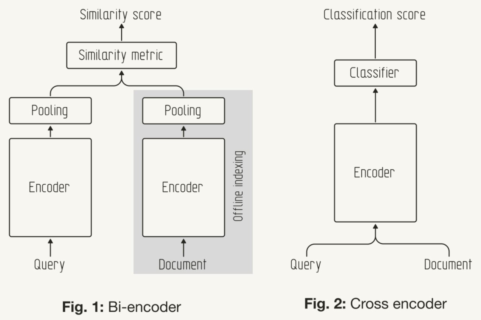
What are the pros and cons of Gradient Boosting Decision Trees?
- Gradient Boosting Decision Trees (GBDT) is a powerful and widely used machine learning technique, particularly for tasks like classification and regression. It builds an ensemble of decision trees in a sequential manner to optimize predictive performance.
- GBDT is a highly effective machine learning algorithm with several advantages in terms of predictive accuracy, flexibility, and minimal preprocessing requirements. However, it comes with trade-offs, including high computational cost, sensitivity to hyperparameters, and difficulty in interpreting models. It is widely used in industry but may not be suitable for all tasks, especially those requiring low-latency predictions, real-time learning, or deep interpretability. For tasks where speed, scalability, or explainability are key concerns, alternatives like Random Forest, linear models, or neural networks may be more appropriate.
- Below are the detailed pros and cons of GBDT:
Pros of GBDT
- High Predictive Accuracy:
- Boosting Effectiveness: GBDT iteratively improves the model by combining weak learners (decision trees) to form a strong learner. This boosting mechanism focuses on the errors made by previous models, leading to significant improvements in performance.
- Handling Non-Linear Relationships: Since decision trees can model complex, non-linear relationships, GBDT inherits this ability, making it highly effective at capturing intricate patterns in the data.
- Versatile:
- Can Handle Various Types of Data: GBDT works well with both numeric and categorical data. It doesn’t require much data preprocessing, like scaling or normalization, which is often needed for algorithms like SVM or neural networks.
- Applicable to Different Problems: GBDT can be used for classification, regression, and even ranking tasks. Its flexibility makes it a go-to choice for many machine learning problems.
- Built-in Feature Selection:
- Feature Importance: GBDT naturally selects important features during training by focusing on those that reduce the most error. This implicit feature selection is useful when dealing with high-dimensional data.
- Automatic Handling of Irrelevant Features: By focusing on areas where the model performs poorly, GBDT downweights irrelevant or noisy features without explicit feature elimination methods.
- Handling Missing Data:
- Missing Values Tolerance: GBDT can handle missing values quite effectively by splitting on missing data as part of the decision-making process, reducing the need for imputation.
- No Need for Extensive Data Preprocessing:
- Minimal Data Transformation: GBDT does not require heavy transformations like normalization, standardization, or one-hot encoding for categorical variables, making it easier to implement on raw data compared to other algorithms.
- Effective with Limited Hyperparameter Tuning:
- Out-of-the-box Performance: GBDT algorithms, particularly modern implementations like XGBoost, LightGBM, and CatBoost, often perform reasonably well with default settings. With fine-tuning, they can be pushed to achieve very high performance.
- Ensemble Learning:
- Combining Weak Learners: GBDT combines multiple decision trees (weak learners), leading to improved generalization by reducing variance and bias compared to a single decision tree.
Cons of GBDT
- Computationally Expensive:
- High Training Time: GBDT builds trees sequentially, meaning each tree depends on the results of the previous one. This sequential nature increases training time, especially on large datasets.
- Memory Consumption: Due to the large number of trees generated in the boosting process, GBDT can require significant memory resources, particularly if the depth of trees is large.
- Sensitive to Hyperparameters:
- Tuning Complexity: While GBDT can perform well out of the box, fine-tuning is often required to get the best performance. Key hyperparameters like learning rate, number of trees, tree depth, and minimum samples per split need careful optimization.
- Risk of Overfitting: If the number of trees is too high or the learning rate is too low, the model can overfit to the training data. Thus, finding a good balance between model complexity and regularization is crucial.
- Difficult to Interpret:
- Black Box Nature: Although decision trees are relatively interpretable, an ensemble of hundreds or thousands of trees is much harder to interpret. This makes GBDT less explainable than simpler models like linear regression or a single decision tree.
- Harder for Stakeholders to Understand: In real-world applications, where explainability is important (e.g., in healthcare or finance), GBDT models may be difficult to justify to non-technical stakeholders.
- Lack of Online Learning Capability:
- Cannot Learn Incrementally: GBDT models are trained in batches, and once trained, they cannot easily accommodate new data without retraining from scratch. This makes them unsuitable for real-time learning or applications requiring frequent model updates.
- Sensitivity to Noisy Data:
- Noise Amplification: GBDT can sometimes amplify the effects of noise in the data. Since each tree attempts to fix errors made by the previous tree, any overfitting to noisy patterns can propagate through the model.
- Requires Careful Handling of Imbalanced Data:
- Less Effective on Imbalanced Datasets: GBDT does not inherently handle class imbalances well. Special techniques like adjusting the loss function, using weighted data, or applying sampling strategies are often needed to mitigate this issue.
- Long Inference Times:
- Prediction Speed: GBDT’s prediction speed can be slow, especially with a large number of trees or deep trees. This can make it less suitable for low-latency applications, where real-time or near-real-time predictions are required.
- Limited Extrapolation Beyond Training Data:
- Poor Extrapolation: Like decision trees, GBDT models struggle with data points that fall outside the range of the training data (extrapolation). For example, they are not well-suited for problems where future trends need to be predicted based on past data (e.g., time series forecasting with far horizons).
Why are GBDTs highly effective with sparse data?
-
GBDTs are highly effective with sparse data, which is a common scenario in recommender systems. Sparse data arises because not all users interact with all items, leading to a matrix where most entries are empty or zero (the interaction matrix). Sparse data is often composed of categorical features that are one-hot encoded or indicator variables for specific interactions, such as a user clicking on or purchasing an item. Details below:
-
Handling of Categorical Features: GBDTs can handle sparse data by splitting decision trees based on subsets of categorical features (e.g., item category, user age group, device type) without needing to densify the data. Unlike models that require continuous data or complex transformations, GBDTs can process one-hot encoded categorical features directly, which is useful for large and sparse interaction matrices.
-
Robust to Missing Values: GBDTs can handle missing data natively. In sparse matrices, many features may be missing or set to zero. GBDT algorithms like XGBoost, LightGBM, and CatBoost include mechanisms to split nodes based on missing values or treat missing values as a distinct feature. This makes them robust and efficient when dealing with datasets where not every feature is fully populated, which is common in recommender systems.
-
Automatic Feature Selection: GBDTs are naturally good at ignoring irrelevant or less informative features. In sparse data settings, many features (e.g., certain user interactions) might not contribute significantly to the predictive power of the model. GBDTs can automatically focus on the features that provide meaningful splits in the data, effectively managing sparsity without overfitting to noise.
-
Non-linear Interactions: GBDTs excel in capturing complex, non-linear relationships between sparse features. For example, a user’s interaction with an item might depend on specific, rare combinations of attributes (like purchasing behavior in a specific geographic location for a particular product type). GBDTs can learn these non-linear patterns without needing extensive feature engineering.
-
How GBDTs Handle Sparse Data
-
One-hot Encoding: GBDTs do not require dense representations of data. Features like user-item interactions can be represented with sparse one-hot encodings, where only a few features are “active” (non-zero) for a given observation. GBDTs can split on any of these one-hot features, allowing them to work directly with the sparse matrix.
-
Efficient Splitting: During the tree-building process, GBDTs evaluate all possible splits at each node, even when the data is sparse. The decision tree will learn to split on meaningful sparse features, helping the model capture useful patterns from high-dimensional, sparse datasets.
-
Categorical Encoding: Algorithms like CatBoost are specifically designed to handle categorical variables more efficiently than traditional one-hot encoding, further improving GBDTs’ performance on sparse data by reducing dimensionality and preserving information.
Why are Gradient Boosting Decision Trees inefficient for Continual/Online Learning?
- Gradient Boosting Decision Trees are inefficient for continual or online learning, which is a significant drawback in dynamic environments like recommender systems. In many real-world recommendation applications, user preferences and item availability change frequently. Continual or online learning refers to a model’s ability to adapt to new data in real time, without retraining from scratch. GBDTs, however, are
-
While GBDTs are powerful for handling sparse data and structured features, their inefficiency in continual or online learning environments limits their application in scenarios that require real-time adaptability. This inefficiency arises because GBDTs are typically batch learners that operate on static datasets and need to be retrained fully to incorporate new information. The computational demands of retraining make them less ideal for fast-evolving recommender systems where new data continuously flows in. Details below:
-
Batch Learning Nature: GBDTs are built in stages by sequentially adding trees, where each new tree corrects the errors made by the previous ones. This is fundamentally a batch learning process because the model is trained on the full dataset, and any new data requires retraining from scratch or restarting the boosting process. This retraining is computationally expensive and time-consuming in systems where new interactions (e.g., user clicks or purchases) are constantly streaming in.
-
Lack of Incremental Updates: Unlike algorithms such as matrix factorization or certain neural network architectures, GBDTs do not have native support for incremental learning (i.e., updating the model without retraining). For every new batch of data, the entire model must be updated to incorporate new patterns, which is not feasible in environments where immediate updates are required.
-
High Computational Overhead: Training GBDTs involves iterative rounds of tree building, where each tree is constructed based on the residuals of the previous iteration. This requires accessing the entire dataset, making it costly to retrain in real-time or with frequently arriving new data. For example, if a recommender system sees new interactions every minute, retraining a GBDT on each new batch of data would significantly slow down the system’s ability to make timely recommendations.
-
How This Inefficiency Manifests
-
Latency in Real-Time Systems: In online or real-time recommender systems, the goal is to quickly adapt to a user’s most recent interactions (e.g., purchases, clicks) to improve the accuracy of recommendations. GBDTs cannot efficiently process this continual stream of new data without retraining the model, leading to latency issues in deploying real-time updates.
-
Resource-Intensive Retraining: In scenarios where retraining is done to accommodate new data, the process can become computationally expensive. Large-scale recommender systems with millions of users and items can’t afford to constantly retrain GBDTs without slowing down the recommendation process. In contrast, methods like stochastic gradient descent (SGD) in matrix factorization or online learning variants of neural networks can update model parameters with each new data point, providing more agile learning capabilities.
Workarounds and Alternatives
- While GBDTs are inherently inefficient for online learning, several workarounds are sometimes employed:
- Mini-batch Retraining: Instead of retraining the model on every new interaction, GBDTs can be retrained periodically (e.g., once every hour or day) in a batch-processing manner. This reduces computational load but sacrifices immediate responsiveness.
- Hybrid Models: To tackle the inefficiency of GBDTs in online learning, many recommender systems employ a hybrid approach, where GBDTs are used in combination with models that can perform real-time updates (e.g., online collaborative filtering models or reinforcement learning-based models). GBDTs can handle complex feature interactions offline, while the other models adjust dynamically to recent interactions.
Are the top/deep layers of the model closer to the final layer or the first layer?
-
In the context of deep neural networks, the top/deep layers refer to those layers that are closer to the final layer (the output layer), not the first layer (the input layer).
-
Here’s how this terminology is typically understood:
- Top/Deep Layers: These are the higher, more specialized layers closer to the output of the model. They learn high-level, task-specific features and representations, such as object classes in image recognition or specific linguistic patterns in text classification.
- Bottom Layers: These are the layers closest to the input. They usually capture more general, lower-level features, such as edges, textures, or general linguistic embeddings. These layers are often more universal across tasks and datasets.
Why Fine-Tuning Often Focuses on Top/Deep Layers
- When fine-tuning a pre-trained model, the top/deep layers are typically modified because:
- They contain more task-specific information from the original training dataset.
- Adjusting these layers helps adapt the model to the new task without disrupting the foundational, general features learned by the lower layers.
- Freezing the bottom layers while fine-tuning the top/deep layers is common practice, as it can reduce overfitting while allowing the model to adjust to new data.
In the context of fine-tuning deep neural networks, can increasing the number of layers make the model more prone to overfitting?
-
In deep neural networks, increasing the number of layers can make the model more prone to overfitting, especially during fine-tuning. Here’s why:
-
Increased Model Capacity: Adding more layers increases the model’s capacity to learn complex patterns. While this can improve performance on the training set, it can lead the model to “memorize” the training data rather than generalize from it, making it less effective on unseen data.
-
More Parameters: With more layers, the number of parameters grows significantly. Fine-tuning such a large model can easily lead to overfitting if there’s insufficient data or if the data lacks variability. In cases of limited data, the model might latch onto noisy patterns that aren’t generalizable.
-
Gradient Amplification and Feature Sensitivity: When fine-tuning deeper layers, gradients tend to amplify, which can make the model overly sensitive to training data. This sensitivity can result in overfitting to specific patterns in the training set that don’t generalize to the test set.
-
Less Regularization on Lower Layers: Fine-tuning more layers often means adjusting lower layers that originally learned more general features (like edges and textures in images). By fine-tuning them, these layers might lose their general-purpose features, over-specializing them to the fine-tuning dataset.
-
Mitigating Overfitting in Fine-Tuning
- To reduce overfitting in deep networks during fine-tuning:
- Use Dropout: Introduce dropout layers to prevent co-adaptation of neurons.
- Regularization: Apply \(L_2\) regularization (weight decay) to discourage excessive weights.
- Layer Freezing: Fine-tune fewer layers or only the top layers of the model.
- Data Augmentation: Expand the effective size of the training dataset by using transformations like cropping, rotation, and color adjustments, especially for image data.
- Fine-tuning deep networks is effective, but managing overfitting is crucial, especially with deeper architectures and smaller datasets.
How does adding a component to the loss term prevent overfitting with regularization?
- Adding a component to the loss term for regularization helps prevent overfitting by penalizing overly complex models, encouraging simpler ones that generalize better to unseen data. Regularization techniques like \(L_1\) (Lasso) and \(L_2\) (Ridge) regularization introduce a penalty term in the loss function, which limits the size or complexity of model parameters. By controlling model complexity, regularization encourages the model to focus on generalizable patterns rather than specific data points, making it less sensitive to the idiosyncrasies of the training data.
- Here’s how this works in detail:
- Penalizing Large Weights:
In models like neural networks or linear regressions, overfitting often involves assigning high weights to certain features, which makes the model sensitive to noise in the training data.
- Regularization adds a term to the loss function (e.g., \(\lambda \sum_{i} w_i^2\) for \(L_2\) regularization) that penalizes large weights. By keeping weights smaller, the model learns a smoother mapping that’s less likely to fit noise.
-
Balancing Fit with Complexity: The regularization term adds a trade-off in the loss function between fitting the training data well and keeping the model complexity in check. For instance, with a regularized loss function \(\text{Loss} = \text{MSE} + \lambda \sum_{i} w_i^2\), the regularization strength \(\lambda\) controls how much weight is given to reducing error versus limiting model complexity. A well-chosen \(\lambda\) helps the model to capture only the significant patterns, not the noise.
-
Improved Generalization: By limiting the capacity of the model to learn very specific mappings, regularization helps the model to generalize better to new data. Overly flexible models tend to memorize training examples, while regularized models are forced to learn broader trends, which results in better performance on validation or test datasets.
- Types of Regularization Penalties:
- \(L_2\) Regularization (Ridge): Penalizes the square of the weights, encouraging the model to spread weight values across many parameters rather than making any one parameter large. This results in smoother models.
- \(L_1\) Regularization (Lasso): Adds an absolute penalty (e.g., \(\lambda \sum_{i} \|w_i\|\)), encouraging sparse models by pushing some weights to zero. This can also perform feature selection by removing less useful features.
Does an LLM produce different outputs for the same input across different iterations? If so, how?
- Yes, an LLM can produce different outputs for the same input across different iterations, depending on how it’s configured. Here’s a breakdown of why and how this variation can occur:
Temperature Setting
- What It Is: “Temperature” is a parameter that controls the randomness of the model’s output. Higher temperatures (e.g., 1.0 or higher) make the output more random, while lower temperatures (e.g., close to 0) make it more deterministic.
- How It Affects Outputs: At high temperatures, the model is more likely to choose from a broader range of possible tokens, leading to more varied responses. At low temperatures, it favors the most probable tokens, which tends to produce similar or identical outputs across runs. This allows for tuning between creative, diverse responses and reliable, consistent ones.
Top-k and Top-p Sampling
- What It Is: These are other mechanisms for controlling randomness. Top-k sampling restricts the model to only the top k most probable tokens at each step, while top-p (nucleus) sampling restricts it to the smallest set of tokens whose cumulative probability reaches a certain threshold (like 0.9).
- How It Affects Outputs: With higher k or p values, the model has a wider range of tokens to choose from, introducing more variability. With lower values, it restricts to more predictable choices, leading to more consistent responses.
Random Seed Initialization
- What It Is: The generation of text in many LLMs involves randomization based on a seed. If the seed is different each time (either explicitly or implicitly set), the model can produce varied outputs for the same prompt.
- How It Affects Outputs: By changing the seed, you effectively alter the “starting point” for the model’s generation, which can lead to different word choices and sentence structures, even with the same prompt.
Context Sensitivity in Extended Interactions
- What It Is: In a multi-turn conversation, LLMs keep track of previous interactions to maintain context. This means that repeated prompts might lead to varied responses if they follow different conversational histories.
- How It Affects Outputs: The same prompt could yield different responses if the surrounding context or conversational “history” changes, as the model adjusts its output to align with the flow of conversation.
Model Size and Fine-Tuning
- What It Is: Larger models with more parameters or those that have been fine-tuned on extensive, diverse datasets tend to have richer response variability.
-
How It Affects Outputs: Larger models, or those fine-tuned for creativity, may naturally produce a broader array of outputs because they have encoded a more nuanced understanding of language patterns and contexts. Smaller or narrowly fine-tuned models may give more predictable results.
- By adjusting these parameters, users or developers can control how much variety an LLM will exhibit, from highly creative and varied outputs to reliable, nearly identical responses.
Explain how random seed initialization works with LLMs.
- In large language models, controlling the random seed is a powerful way to manage and reproduce variations in text generation. Here’s how it works and how you can implement it in code:
What is a Seed?
- A random seed is a starting point for the sequence of random numbers generated by the model. When using a random seed, the model’s token sampling will follow a predictable pattern if the same seed is reused, making it easy to reproduce results. However, when the seed changes, the sequence becomes different, leading to varied outputs.
How to Control the Random Seed in Code
- Let’s look at two common libraries where setting the seed is possible: OpenAI’s API (for models like GPT-3/4) and Hugging Face’s Transformers library (for local or custom models).
Using OpenAI’s API
-
The OpenAI API currently does not provide direct control over the random seed in text generation calls, but you can simulate the effect by controlling other parameters (like temperature, top-p, etc.) or by pre-generating random seeds in your code and structuring the API call around them.
-
In Python, you could create a function that sets a seed value by manipulating other factors within your code (such as the prompt or randomizing other parameters). Here’s an example of how you might approach it:
import openai
import random

def generate_with_seed(prompt, seed=None):
    if seed is not None:
        random.seed(seed)  # Set Python's random seed to ensure reproducibility.
        # Optional: set a unique suffix based on the seed
        prompt += f" Seed-{seed}"

    response = openai.Completion.create(
        model="text-davinci-003",
        prompt=prompt,
        max_tokens=100,
        temperature=0.7  # adjust this for variability
    )
    return response.choices[0].text

# Usage
prompt = "Once upon a time in a distant land"
seed = 42  # Set any integer for reproducibility
output = generate_with_seed(prompt, seed)
print(output)
- While OpenAI’s API doesn’t use
seeddirectly, adding aseed-specific prompt suffix could effectively simulate a controlled variance.
Using Hugging Face’s Transformers Library
- The Transformers library by Hugging Face allows you to set a seed directly, making it easier to achieve deterministic output. Here’s how it works:
from transformers import pipeline, set_seed

# Load a text generation pipeline
generator = pipeline('text-generation', model='gpt2')

def generate_with_seed(prompt, seed=None):
    if seed is not None:
        set_seed(seed)  # This will control randomness in the model's generation

    # Generate text
    result = generator(prompt, max_length=50, num_return_sequences=1)
    return result[0]['generated_text']

# Usage
prompt = "Once upon a time in a distant land"
seed = 42  # Any integer to set the random seed
output = generate_with_seed(prompt, seed)
print(output)
- In this case,
set_seed(seed)fixes the random seed, ensuring that every time you run the function with the same seed, you’ll get the same output. Changing the seed each time will lead to different outputs.
Explanation of How the Seed Alters Generation
-
Set the Seed: By calling
set_seed(seed)(or any equivalent method), you initialize the random number generator with a specific value. -
Sampling: During text generation, the model selects tokens based on probability distributions. The seed controls how these probabilities are interpreted and which token is chosen at each step.
-
Repeatability: If you run the code with the same prompt and seed, the model’s choices will follow the same path through the probability distribution, producing identical outputs. Change the seed, and this path shifts, creating a new sequence of tokens and thus different outputs.
Practical Example: Changing Seed for Diverse Outputs
# Generate multiple outputs with different seeds
prompt = "The sun was setting over the calm ocean"
seeds = [1, 2, 3, 4]

for seed in seeds:
    output = generate_with_seed(prompt, seed)
    print(f"Seed {seed}: {output}\n")
- By iterating over different seed values, you’ll see distinct outputs for each seed. Each seed provides a unique “starting point” for the model’s token sampling, which impacts the final response.
Why This Matters
- Using seeds effectively allows developers to:
- Control variability: Useful for tests or specific scenarios where repeatability is needed.
- Generate diverse content: Varying seeds can create unique responses for creative applications.
- Debug and analyze outputs: If a particular output is interesting or problematic, using the same seed helps reproduce and analyze it.
- This ability to set and change seeds gives you a robust handle on both predictability and variety in LLM outputs.
How does the seed impact the LLM sampling using transformers library?
- When using the Transformers library, the random seed directly impacts the sampling process of a large language model (LLM) by determining how the model selects tokens based on their probability distributions. Here’s a detailed look at how it works and why the seed influences the output:
Understanding Token Sampling in LLMs
-
In language generation, an LLM predicts the next word (or token) by assigning probabilities to all possible tokens. For example, given a partial sentence like “The cat sat on the…”, the model calculates probabilities for likely next words, such as “mat,” “sofa,” “floor,” etc. The sampling mechanism then decides which word to choose based on these probabilities.
- Sampling Methods in Transformers Library:
- Greedy Sampling: Always picks the most probable token.
- Beam Search: Considers multiple top paths to choose a sequence.
- Top-k Sampling: Limits choices to the top k tokens, adding randomness by choosing among the k most probable tokens.
- Top-p Sampling (Nucleus Sampling): Selects tokens from the smallest possible set where cumulative probability reaches a threshold (p), often 0.9.
- With random sampling (such as top-k or top-p), the selection process is influenced by randomness, which is where the random seed comes in.
Role of the Seed in Sampling
-
The seed initializes the random number generator that determines which tokens are chosen during sampling. Here’s how it affects each step in the process:
- Random Initialization: By setting the seed, you fix the starting point of the random number generator, making the process deterministic for that seed value.
- Token Choice: In top-k or top-p sampling, the model picks among several likely tokens. The random seed affects which of these tokens is ultimately chosen. For example, if “mat,” “sofa,” and “floor” are all probable next tokens, the seed influences which one is selected, even though all have similar probabilities.
- Consistency: If the seed remains the same, the sequence of “random” choices stays the same, meaning the model will consistently choose the same tokens at each step, leading to identical outputs for the same input prompt. Changing the seed, however, alters these choices and produces a different sentence structure or wording.
Implementation in the Transformers Library
-
In the Transformers library, setting the seed is straightforward, typically done using
transformers.set_seed(seed). Here’s what happens internally: -
When you call
set_seed(seed), it sets the seed for Python’srandommodule, NumPy’s random generator, and any other random functions used by the model. This ensures that all parts of the token-sampling process operate with the same random seed.
from transformers import pipeline, set_seed

# Load a text generation pipeline
generator = pipeline('text-generation', model='gpt2')

# Set the seed to control randomness
set_seed(42)
- Once the seed is set, any subsequent generation calls will be deterministic for that seed, meaning every time you run the generation with the same prompt and seed, you’ll get the same output.
How the Seed Changes Output Diversity
- Changing the seed allows you to explore different continuations of the same input prompt without changing the model’s parameters or re-running it. Each unique seed will lead to a different series of “random” choices among the top-k or top-p tokens, producing varied outputs in terms of:
- Word choice: Different synonyms or related terms may be chosen.
- Sentence structure: The model may follow different paths in phrasing or sentence continuation.
- Tone and Style: Subtle changes in word choice can shift the tone, making it more formal or casual, depending on the sampled tokens.
- Here’s an example that illustrates how changing the seed can impact the output:
prompt = "The future of AI is both exciting and"

# Generate with different seeds
for seed in [1, 42, 99]:
    set_seed(seed)
    output = generator(prompt, max_length=50, num_return_sequences=1)
    print(f"Seed {seed}: {output[0]['generated_text']}\n")
Use Cases for Seed Control in LLMs
- Setting a seed has practical benefits:
- Repeatability: By fixing the seed, you can reproduce specific results, making it easier to test, debug, or analyze certain outputs.
- Content Variation: By altering the seed, you can generate diverse outputs from the same model and prompt without re-training or modifying other parameters.
- Controlled Randomness in Creative Tasks: You can achieve creative and varied outputs by simply cycling through different seeds, which is especially useful for applications like story generation, marketing copy, or dialogue creation.
- In summary, the seed acts as a way to “anchor” the model’s randomness, guiding the token-sampling process in a controlled yet flexible way. By setting and changing seeds, you can explore a spectrum of possible outputs for the same input prompt, balancing predictability and creative variation.
What does it mean for an ML model to be non-parametric?
-
In machine learning, a non-parametric model is one that doesn’t assume a fixed number of parameters. Unlike parametric models, which have a predetermined structure (such as linear regression with fixed coefficients), non-parametric models adapt their structure based on the complexity and amount of data they have. Here are some key points about non-parametric models:
-
Flexibility with Data Size: Non-parametric models grow more complex as the amount of data increases. Instead of summarizing the data in a fixed set of parameters, they may use the data directly, allowing for a more flexible model that can capture a wide range of patterns and relationships.
-
No Assumptions About Data Distribution: Non-parametric models don’t require assumptions about the underlying data distribution (such as being linear, Gaussian, etc.). This makes them useful in cases where the relationship between features is complex or unknown.
- Examples of Non-Parametric Models:
- K-Nearest Neighbors (KNN): This model directly uses the training data to make predictions by finding the “k” most similar instances.
- Decision Trees: Decision trees can grow in complexity depending on the data, splitting based on criteria that maximize the information gain at each level.
- Kernel Density Estimation (KDE): KDE is used for estimating the probability density function of a random variable without assuming a specific parametric form.
- Trade-offs:
- More Data Dependency: Non-parametric models may require more data to accurately capture patterns, as they rely on the data itself rather than summarizing it in a few parameters.
- Computationally Intensive: Since non-parametric models often need to reference or compare to much of the training data at prediction time, they can be slower and more memory-intensive.
- Overfitting Risk: Because non-parametric models can adapt closely to the data, they are sometimes more prone to overfitting, especially if not regulated by techniques like pruning (in trees) or limiting “k” in KNN.
-
-
In summary, non-parametric models are powerful for handling complex data patterns without rigid assumptions, but they require careful tuning and enough data to generalize well.
Which ML algorithms are non-parametric?
- Non-parametric machine learning models are those that do not make strong assumptions about the form of the underlying data distribution, meaning they do not rely on a fixed number of parameters. Instead, the number of parameters grows with the amount of data, allowing them to adapt more flexibly to the data. Some well-known non-parametric models include:
- K-Nearest Neighbors (K-NN):
- Does not assume any specific structure in the data. It classifies a new data point based on the classes of its closest neighbors, with the number of neighbors often specified by a hyperparameter.
- Decision Trees:
- Can be considered non-parametric since they split data based on feature values without a pre-set structure. The tree grows based on the data until a stopping condition is met, making it highly adaptable.
- Random Forests and Bagging:
- Ensembles of decision trees are also non-parametric as they aggregate multiple non-parametric decision trees to make a prediction. Each tree in the forest adjusts based on different subsets of the data.
- Support Vector Machines (with non-linear kernels):
- With non-linear kernels, SVMs can be non-parametric, as the number of support vectors used can grow with the data, allowing it to model complex decision boundaries without a fixed parameter set.
- Gaussian Processes:
- A flexible, non-parametric Bayesian approach where predictions are distributions that adapt to data patterns. The model complexity grows with the number of data points.
- Kernel Density Estimation (KDE):
- Used for estimating the probability density function of a random variable without assuming a particular distribution form. KDE is data-driven and can adapt to complex data structures.
- Neural Networks (sometimes considered):
- Though typically seen as parametric, certain architectures, such as deep neural networks with many layers, can approximate non-parametric behavior in practice because they adapt flexibly to data and often have many more parameters than simpler models.
- Non-parametric models are generally more flexible and better at capturing intricate patterns in data, but they may require more data and computational resources than parametric models to make accurate predictions.
Is k-means clustering parametric?
-
Yes, k-means clustering is generally considered a parametric model, not a non-parametric one. Here’s why:
-
Fixed Number of Parameters: In K-means, the number of clusters \(K\) is predetermined, meaning that the model has a fixed number of parameters (the centroids of the clusters) regardless of the data size. This differs from non-parametric models, which adapt their complexity based on the amount of data available.
-
Centroid-based Structure: K-means clustering represents each cluster with a centroid, which is computed as the mean of points within the cluster. The model assumes that clusters are roughly spherical around these centroids and that each data point belongs to the nearest centroid.
-
Rigid Assumptions: K-means clustering makes specific assumptions about the structure of the data, particularly that clusters are isotropic and separable based on distance (typically Euclidean distance).
-
- In contrast, non-parametric clustering techniques, like DBSCAN (Density-Based Spatial Clustering of Applications with Noise) or hierarchical clustering, don’t require a fixed number of clusters. DBSCAN, for instance, identifies clusters based on data density and can adjust to data with varying shapes and densities, which is characteristic of non-parametric models.
- So, while K-means is a powerful clustering algorithm, it is not considered non-parametric because of its reliance on a fixed, predetermined number of clusters and specific assumptions about data structure.
What is an isotropic cluster?
-
An isotropic cluster is a type of cluster in which data points are distributed uniformly in all directions around a central point, usually forming a roughly spherical or circular shape. The key characteristics of an isotropic cluster are:
-
Equal Variance in All Directions: In an isotropic cluster, the spread of data points is the same in every direction from the center. This means the variance along any axis or dimension is equal.
-
Spherical (or Circular) Shape: In a two-dimensional space, isotropic clusters tend to be circular, while in higher dimensions, they form spherical clusters. The data points are distributed around the cluster center at a similar distance, forming a ball-shaped distribution.
-
Distance-based Clustering Assumptions: Algorithms like K-means clustering assume isotropic clusters because they use Euclidean distance to assign points to the nearest centroid. This assumption works well when clusters are spherical, as Euclidean distance effectively captures proximity to the cluster centers.
-
Contrast with Anisotropic Clusters: An anisotropic cluster has a spread that varies across different directions, which can result in ellipsoidal shapes or elongated clusters. Anisotropic clusters do not have uniform variance in all directions.
-
Example
-
Imagine clustering data points in two dimensions:
- Isotropic Cluster: Points are evenly distributed around a central point, forming a circular shape with roughly the same spread in all directions.
- Anisotropic Cluster: Points are distributed in an elongated ellipse, with a greater spread in one direction than the other.
-
Isotropic clusters are simple and computationally convenient, but real-world data often have anisotropic structures, which require more flexible clustering methods, like Gaussian Mixture Models or DBSCAN, that can adapt to clusters with non-spherical shapes.
What are alpha experiments for feature selection in ML model training?
- Alpha experiments, particularly in the context of machine learning and feature selection, refer to early-stage testing and exploration of potential features to include in a predictive model. These experiments are typically used to assess the impact of individual features or combinations of features on model performance before committing to a full model development and evaluation cycle. Here are some common alpha experimental approaches and techniques for feature selection in machine learning:
Single-Feature Testing
- Objective: Quickly assess whether a feature has any predictive power.
- Method: Train simple models using only one feature at a time. This can be done with lightweight models (like linear regression or decision trees), using each feature individually to see if it yields any predictive performance. This approach is a quick way to determine whether any given feature adds value on its own.
Correlation Analysis
- Objective: Identify potentially redundant features.
- Method: Use correlation matrices or other statistical measures (such as mutual information) to identify pairs of features that are highly correlated. Redundant features can inflate model complexity and may not add value, so alpha experiments can help identify features to drop early on.
Forward and Backward Selection
- Objective: Incrementally add or remove features to see their effect.
- Method: In forward selection, start with no features and add them one by one, testing the model’s performance each time. In backward selection, start with all features and remove them one by one. These methods allow for quick experimentation to identify impactful features or subsets.
PCA and Other Dimensionality Reduction Techniques
- Objective: Explore the underlying structure and redundancy of features.
- Method: Principal Component Analysis (PCA) and other dimensionality reduction techniques can help identify which features capture the most variance in the data, potentially reducing the feature space while retaining significant information.
Recursive Feature Elimination (RFE)
- Objective: Test combinations of features by iteratively removing less important ones.
- Method: Use RFE with a simple model to rank features by importance. This method eliminates the least important feature(s) in each iteration and re-evaluates the model. This iterative approach can be a quick way to identify a subset of features that improves performance, making it suitable for alpha-stage feature selection.
Univariate Feature Selection
- Objective: Rank features based on statistical significance.
- Method: Use statistical tests (such as ANOVA, chi-square, or t-tests) to evaluate the relationship of each feature with the target variable individually. Selecting features with high scores provides a quick, univariate assessment of the feature’s potential value.
Feature Importance with Tree-Based Models
- Objective: Quickly determine feature importance in nonlinear models.
- Method: Use a simple tree-based model (like a Decision Tree or a small Random Forest) to obtain feature importance scores. Many tree-based models automatically rank features based on their importance, allowing you to test which features contribute most to model performance in alpha experiments.
Regularization Techniques (L1 and L2)
- Objective: Perform feature selection by penalizing complexity.
- Method: Use regularized linear models (such as Lasso for L1 regularization and Ridge for L2 regularization) to identify features that contribute the most predictive power while reducing the effect of less important features. L1 regularization can even reduce the coefficients of some features to zero, effectively performing feature selection.
Permutation Feature Importance
- Objective: Test the robustness of each feature’s contribution.
- Method: Shuffle the values of each feature in turn and observe the impact on model performance. Features that cause a significant drop in performance when permuted are likely more important, helping identify which features are essential at an early stage.
Synthetic Feature Generation and Interaction Testing
- Objective: Test interaction effects and derived features.
- Method: Create new features by combining existing ones (like ratios, sums, or polynomial combinations) and test their impact on the model. This can reveal non-obvious interactions that may improve performance and is especially useful for identifying candidate features for later stages.
Feature Selection Based on Stability Scores
- Objective: Test feature consistency across different datasets.
- Method: Train the model on different subsets of data or through cross-validation, recording feature importance scores for each subset. Features with high variance in importance scores may be unreliable, so identifying stable features early on can improve model robustness.
Best Practices for Alpha Feature Selection Experiments
- Use lightweight models to quickly test and iterate over features without overfitting.
- Automate experiments where possible, using pipelines that can test multiple feature combinations, track results, and highlight impactful features.
- Validate across subsets of data (cross-validation) to avoid overfitting to specific feature subsets.
-
Document results for each experiment, noting feature performance for future refinement in subsequent beta and production phases.
- Alpha feature selection experiments aim to narrow down a large feature set to a manageable, high-potential subset that can be tested in depth in later stages, ultimately improving model performance, interpretability, and robustness.
What are beta experiments in ML model training?
- Beta experiments represent a pivotal phase in the ML model development lifecycle, following the initial “alpha” experimentation stage. While alpha experiments are typically exploratory, covering a wide range of possibilities, beta experiments shift focus toward refining and validating the model under more realistic conditions. In this phase, the model is closer to its final form, with selected features and configurations tested in a structured and rigorous manner. The goal of beta experiments is to ensure that the model is robust, generalizable, and suitable for deployment.
- By thoroughly validating and refining the model, beta experiments act as a bridge from early experimentation to production. This stage is critical to confirm that the model will deliver consistent, high-quality performance in real-world applications, making it reliable, resilient, and ready for deployment.
Key Objectives of Beta Experiments
- Feature Validation and Refinement:
- After selecting promising features in alpha experiments, beta experiments validate their effectiveness in various conditions. This stage confirms that selected features consistently contribute to model performance across diverse data scenarios.
- Hyperparameter Tuning:
- Beta experiments involve fine-tuning hyperparameters to optimize model performance. This can include testing different configurations for parameters such as learning rate, regularization strength, maximum depth (in tree models), and others, depending on the model type.
- Generalization Testing:
- Beta experiments aim to ensure that the model generalizes well to unseen data. This includes testing on held-out data, cross-validation, and potentially testing on a more representative sample of real-world data to assess performance under conditions that mirror deployment.
- Bias and Fairness Evaluation:
- An essential part of beta testing is checking the model for any unintended biases or fairness issues. This might involve analyzing model performance across different demographic groups or other subsets to ensure that the model predictions are fair and equitable.
- Stability and Robustness Testing:
- Beta experiments evaluate the model’s stability, checking whether it provides consistent performance across different data subsets and configurations. Techniques like stability testing across random seeds or across different data sampling techniques are commonly used to ensure robustness.
- Scalability and Efficiency Testing:
- At this stage, model training and inference performance are assessed for efficiency and scalability. This can include analyzing training time, inference speed, and resource requirements to ensure the model will meet the operational demands in production.
Techniques and Approaches in Beta Experiments
- Cross-Validation with Hyperparameter Tuning
- Use cross-validation (such as k-fold or stratified k-fold) to evaluate model performance more comprehensively across different subsets of the training data. Coupling this with grid search or random search for hyperparameter tuning ensures optimal parameter values are chosen without overfitting.
- Automated Hyperparameter Optimization (Bayesian Optimization)
- Techniques like Bayesian optimization, Hyperband, or Tree-structured Parzen Estimator (TPE) can be employed to find the best hyperparameters more efficiently than a simple grid or random search, especially for complex models or larger datasets.
- Feature Interaction and Polynomial Feature Testing
- To ensure no valuable interaction is overlooked, beta experiments often involve generating interaction features (e.g., pairwise products or polynomials) among selected features. Testing these interactions can reveal additional improvements in predictive performance, particularly for complex relationships.
- Regularization Tuning and Model Pruning
- Regularization parameters (such as L1, L2 for linear models or tree pruning for tree-based models) are fine-tuned to balance complexity and generalizability. This helps prevent overfitting and keeps the model simpler and more interpretable.
- Ensemble Methods and Model Stacking
- If a single model is underperforming, beta experiments may involve creating ensembles of models, such as bagging, boosting, or stacking. These techniques combine predictions from multiple models to improve overall performance and robustness, often yielding better results than individual models.
- A/B Testing on Real-World Data
- If possible, beta testing may include limited A/B testing or deploying the model to a small segment of users to evaluate real-world performance. This controlled deployment tests the model’s predictions in live environments, capturing user interactions and feedback that reflect real use cases.
- Model Interpretability and Explainability Testing
- Interpretable models or post-hoc explainability techniques (like SHAP or LIME) are used to understand and verify the behavior of model predictions. This step is essential for ensuring stakeholders understand the model’s decision-making process and can identify any potential biases or logical inconsistencies.
- Sensitivity Analysis
- Sensitivity analysis tests the model’s reaction to small changes in input data, ensuring stability and robustness. For instance, perturbing inputs slightly and observing if the predictions change drastically can indicate an unstable or overly sensitive model that may not perform reliably in production.
- Adversarial Testing
- To assess model robustness, adversarial examples or synthetic variations of inputs can be introduced to evaluate the model’s resilience. Adversarial testing helps ensure the model can handle noise, data shifts, and edge cases without significant performance degradation.
- Bias Detection and Fairness Audits
- During beta testing, the model undergoes bias and fairness analysis. Techniques like disparate impact analysis or group fairness metrics are used to ensure that the model does not unfairly favor or disadvantage any group.
Key Metrics and Performance Evaluation in Beta Experiments
- Precision, Recall, F1-Score, ROC-AUC: Standard classification metrics are often used in beta testing to gauge accuracy, especially for imbalanced datasets where metrics like F1-score and AUC are more informative than accuracy.
- Mean Absolute Error (MAE), Mean Squared Error (MSE), R-squared: These are standard metrics for regression tasks and are crucial for assessing the model’s prediction accuracy.
- Lift and Gain Analysis: Lift and gain charts assess how well the model segments data for binary classification, especially useful in marketing or recommendation systems.
- Calibration: Evaluates whether the predicted probabilities reflect true likelihoods. Calibration is crucial in applications like risk assessment or medical diagnostics where probability estimates must be reliable.
- Fairness and Bias Metrics: Evaluates model performance across different demographic or other critical subgroups, looking for parity or lack of discrimination.
Outputs and Next Steps After Beta Experiments
After beta experiments, you should have a well-tested, fine-tuned model with documented performance metrics, known limitations, and, ideally, explanations for its decisions. At this point, the model is ready for final validation and deployment. The outputs include:
- Refined Model with Optimized Hyperparameters: A trained model with the best hyperparameter values and selected features ready for production.
- Performance and Robustness Report: A comprehensive report detailing the model’s performance metrics, robustness, and stability.
- Explainability and Interpretability Analysis: Documentation on model behavior, feature importance, and explainability results to ensure stakeholders understand how and why predictions are made.
- Deployment Readiness Assessment: Final evaluations on resource requirements, scalability, and integration needs to ensure smooth deployment.
Benefits of Beta Experiments
- Risk Reduction: Beta experiments catch potential issues like overfitting, instability, and biases before deployment.
- Improved Performance and Robustness: Through thorough testing and fine-tuning, beta experiments enhance model performance and ensure it generalizes well.
- Transparency and Trust: By documenting and explaining model behavior, beta experiments build trust with stakeholders and end-users, especially critical for high-stakes applications.
- Deployment Confidence: After passing beta experiments, the model is much more likely to perform as expected in production, reducing post-deployment iterations and adjustments.
Is low bias and variance desirable? What is the Bias-Variance Tradeoff?
-
Yes, achieving low bias and low variance is generally desirable in machine learning because it indicates that a model is both accurate and generalizable. Here’s why each is important:
-
Low Bias: Bias refers to the error due to overly simplistic assumptions in the model. Low bias means the model accurately captures the true relationship in the data. High bias, on the other hand, can lead to underfitting, where the model doesn’t capture the underlying patterns well.
-
Low Variance: Variance refers to the model’s sensitivity to fluctuations in the training data. Low variance means that the model can generalize well to new, unseen data. High variance often leads to overfitting, where the model learns the noise or specific quirks of the training data rather than the underlying patterns, making it less effective on new data.
-
The Bias-Variance Tradeoff
- In practice, there’s a tradeoff between bias and variance, as models with low bias (high complexity) often have higher variance, and models with low variance (low complexity) tend to have higher bias. The ideal model is one that balances these two factors, achieving both low bias and low variance to minimize prediction error on unseen data.
- So, while low bias and low variance are desirable, it can be challenging to achieve both simultaneously, and some balance is often needed based on the specifics of the data and problem.
Is high precision and recall desirable? What is the precision-recall tradeoff?
- Yes, high precision and recall are generally desirable, but they often compete with each other, leading to what is known as the precision-recall tradeoff. Understanding these metrics and their relationship can help clarify this balance.
- Precision and Recall:
- Precision: Measures how many of the items classified as positive are actually positive. High precision means few false positives (FP), so the predictions are accurate when the model says “positive.” \(\text{Precision} = \frac{\text{True Positives (TP)}}{\text{True Positives (TP) + False Positives (FP)}}\)
- Recall: Measures how many actual positive cases the model captures out of all true positive cases. High recall means few false negatives (FN), so the model catches most true positives. \(\text{Recall} = \frac{\text{True Positives (TP)}}{\text{True Positives (TP) + False Negatives (FN)}}\)
- Why both are desirable:
- In many applications, high precision and recall together mean that:
- High precision: Predictions are trustworthy, with minimal false alarms (false positives).
- High recall: The model catches all or most of the positive cases, minimizing missed detections (false negatives).
- However, achieving high precision and recall simultaneously is challenging, which leads to the precision-recall tradeoff.
- In many applications, high precision and recall together mean that:
- The precision-recall tradeoff:
- Increasing one often reduces the other, especially in unbalanced datasets where positives are rare. Here’s why:
- Threshold Adjustment: Many models, especially classification models, use a probability threshold to decide between positive and negative. Adjusting this threshold impacts both precision and recall:
- A higher threshold typically increases precision but reduces recall (fewer predictions overall, but more accurate ones).
- A lower threshold usually increases recall but reduces precision (more predictions overall, with more false positives).
- Application Requirements: Some applications need high precision over recall, while others need high recall over precision:
- High Precision Priority: In scenarios where false positives are costly (e.g., spam detection, where misclassifying legitimate emails as spam is problematic), precision is prioritized.
- High Recall Priority: In situations where missing positive cases is costly (e.g., medical diagnoses, where failing to catch a disease is dangerous), recall is prioritized.
- Balancing Precision and Recall:
- For applications that need a balance, metrics like the F1 Score can be helpful as it is the harmonic mean of precision and recall.
- F1 Score helps optimize both precision and recall simultaneously and is especially useful when dealing with imbalanced datasets.
- Threshold Adjustment: Many models, especially classification models, use a probability threshold to decide between positive and negative. Adjusting this threshold impacts both precision and recall:
- Increasing one often reduces the other, especially in unbalanced datasets where positives are rare. Here’s why:
- Practical examples of the tradeoff:
- In fraud detection, missing a fraud case (low recall) may be more acceptable if it means only clear fraud cases are flagged (high precision).
- In information retrieval or search engines, recall may be more important to ensure users see all relevant results, even if some irrelevant ones appear (accepting lower precision).
- In short, high precision and recall are desirable, but they must be balanced based on the application’s specific needs and the cost of false positives versus false negatives.
What is the Zipf’s law (i.e., Power law)?
- Zipf’s Law is an empirical rule that describes the frequency distribution of elements in various datasets, especially in language and social sciences. Named after linguist George Zipf, the law states that in a large dataset, the frequency of any item is inversely proportional to its rank.
- Here’s how Zipf’s Law typically works:
- If you rank elements in a dataset by their frequency (from most to least common), the frequency of the second-ranked item is about half that of the most frequent item, the third is about a third, and so on.
-
Mathematically, it suggests that the frequency \(f\) of an element with rank \(r\) follows the formula:
\[f(r) \approx \frac{C}{r^s}\]- where \(C\) is a constant and \(s\) is close to 1 in natural language distributions.
Example in Language
- In English, Zipf’s Law applies to word frequency. The most common word (“the”) appears far more frequently than the second most common word (“be”), which appears more frequently than the third (“to”), and so on.
Applications of Zipf’s Law
- Zipf’s Law can be observed in many fields beyond language, including:
- City Populations: The population of the largest city is about twice that of the second-largest, three times that of the third-largest, and so forth.
- Website Popularity: The most visited website gets significantly more traffic than the second most popular, and so on.
- Natural Phenomena: Earthquake magnitudes, the size of moon craters, and even incomes can sometimes follow Zipfian distributions.
Why Zipf’s Law is Important
- Zipf’s Law reveals patterns in complex systems and helps in fields like information theory, linguistics, and data science to make predictions or create models. It highlights an underlying “power-law” distribution common in many natural and social systems, showing that a few items dominate in frequency or size while most others are less frequent or smaller.
What are the most common methods to deal with vanishing gradients?
- The vanishing gradient problem occurs in deep neural networks when gradients become very small during backpropagation, preventing the model from updating effectively and causing layers near the beginning to train very slowly or not at all.
- Each of the below techniques can help address vanishing gradients, either by ensuring gradients don’t diminish as much or by structurally enabling them to bypass challenging parts of the network.
Using ReLU and Variants
- ReLU (Rectified Linear Unit) and its variants like Leaky ReLU, Parametric ReLU (PReLU), and Exponential Linear Units (ELU) help reduce the vanishing gradient problem because they avoid saturation for positive values, unlike sigmoid and tanh activations. ReLU maintains gradients for positive values, allowing better gradient flow through the network.
Batch Normalization
- Batch Normalization normalizes inputs for each layer, keeping activations within a standard range and reducing internal covariate shift. This normalization helps stabilize gradients during backpropagation, making training more efficient and addressing gradient vanishing.
Residual Connections (Skip Connections)
- Residual networks (ResNets) use skip connections, where the input to a layer is added directly to its output. This setup enables gradients to flow more easily back to earlier layers, helping to maintain strong gradient signals even in very deep networks.
Careful Weight Initialization
- Initializing weights properly can mitigate vanishing (and exploding) gradients. Xavier (Glorot) initialization and He initialization (for ReLU and variants) are two techniques that set initial weights to appropriate values based on the network’s architecture. These methods help maintain consistent gradient magnitudes as they propagate through layers.
Using LSTM or GRU in Recurrent Networks
- In recurrent neural networks (RNNs), Long Short-Term Memory (LSTM) units and Gated Recurrent Units (GRU) are designed to mitigate vanishing gradients. They include mechanisms for remembering and forgetting information, which helps gradients flow across time steps without vanishing.
Layer Normalization
- Layer normalization is similar to batch normalization but normalizes across features within each layer individually. It is often used in sequential models and RNNs, providing stability to gradients and improving training efficiency.
Smaller Learning Rates
- A smaller learning rate can help prevent the gradients from becoming too small or too large. While it slows down learning, it can make gradients more stable, especially in networks prone to vanishing gradient issues.
What are the most common methods to deal with exploding gradients?
- Exploding gradients are a common issue in deep neural networks, especially recurrent neural networks (RNNs) and deep feedforward networks, where gradients during backpropagation become excessively large, leading to instability in training and poor model performance.
- The methods listed below are often used in combination to manage gradient magnitudes and stabilize training. In practice, gradient clipping and proper initialization are particularly popular choices, especially in recurrent neural network training where exploding gradients are a more frequent concern.
Gradient Clipping
- Gradient clipping involves setting a threshold value and scaling the gradients if they exceed this threshold. This prevents the gradients from becoming excessively large.
- Common types of clipping include global norm clipping, where gradients are clipped if the overall norm exceeds a certain value, and element-wise clipping, where individual gradient components are clipped to be within a specified range.
- This method is straightforward and widely used in practice, especially in RNNs and other deep architectures.
Weight Regularization (L2 Regularization)
- L2 regularization (weight decay) applies a penalty proportional to the square of the magnitude of weights, which discourages excessively large weights and thus indirectly controls large gradients.
- This technique helps keep weights smaller and gradients more manageable, though it may not be as directly effective on gradient magnitude as gradient clipping.
Using Proper Initialization
- Proper weight initialization can prevent gradients from exploding (or vanishing) at the start of training.
- Techniques like Xavier/Glorot initialization and He initialization help set initial weights in a range that maintains stable gradient magnitudes across layers.
- Choosing the initialization method based on the activation function (e.g., He initialization for ReLU-based networks) can be particularly beneficial.
Batch Normalization
- Batch normalization normalizes the inputs to each layer within a minibatch, keeping activations in a stable range.
- It helps mitigate exploding and vanishing gradient issues by maintaining a consistent distribution of layer inputs, which reduces the likelihood of extremely large or small gradient values.
Use of Appropriate Activation Functions
- Certain activation functions, such as ReLU, tend to exacerbate gradient issues in deeper networks due to unbounded positive outputs.
- Choosing more stable activation functions (e.g., Leaky ReLU, ELU) or even tanh for some RNNs can help by keeping activation values in a more controlled range.
Gradient Norm Penalty
- This method involves adding a penalty term to the loss function based on the gradient norm.
- The penalty discourages excessively large gradients during training by making it costly for the model to reach high gradient values.
- Gradient norm penalties are particularly useful when using generative models or reinforcement learning, where gradient stability is crucial.
Layer Normalization (for RNNs)
- In RNNs, layer normalization (or batch normalization adapted for recurrent structures) helps stabilize training by normalizing across hidden states, preventing gradients from exploding over long sequences.
- Layer normalization is effective when batch normalization is challenging to apply, as is often the case with recurrent networks.
Reduce Learning Rate
- A high learning rate can amplify the problem of exploding gradients. By reducing the learning rate, the network’s parameter updates become more gradual, reducing the risk of large gradient values.
- This approach is often used in conjunction with other methods, such as adaptive learning rate optimizers like Adam or RMSprop, which help adjust learning rates during training.
Skip Connections / Residual Networks
- For very deep networks, skip connections (as in residual networks or ResNets) help gradients bypass layers, allowing for more direct gradient flow and reducing the likelihood of exploding gradients in deeper networks.
- By allowing information to skip certain layers, gradients are less likely to be amplified excessively across layers.
Are Variational Autoencoders (VAEs) and Autoencoders (AEs) typically non-linear?
- Yes, Variational Autoencoders (VAEs) and Autoencoders (AEs) are typically non-linear. Here’s why:
Autoencoders (AEs)
- Autoencoders consist of an encoder and a decoder, which are usually implemented as neural networks.
- The encoder compresses the input into a latent space representation (bottleneck), and the decoder reconstructs the original input from this latent space.
- Non-linear activation functions (e.g., ReLU, sigmoid, tanh) are commonly used between layers of the encoder and decoder. These non-linearities allow the model to capture complex relationships in the data.
- If only linear transformations were used, the Autoencoder would essentially perform a simple Principal Component Analysis (PCA), which is linear. Non-linearity enables AEs to model more complex data distributions.
Variational Autoencoders (VAEs)
- VAEs extend the concept of Autoencoders by incorporating probabilistic modeling, where the latent space is represented as a distribution rather than a fixed vector.
- VAEs also use neural networks for the encoder (which estimates parameters of the latent distribution) and the decoder (which generates samples from the latent space to reconstruct the data).
- Non-linearities in the neural networks enable the VAE to learn and generate from complex, non-linear data distributions.
- In both cases, non-linearity is a fundamental feature that makes these models powerful for tasks like dimensionality reduction, generative modeling, and capturing intricate data patterns.
What is the relationship between LDA and VAE in terms of representing the latent space as a distribution rather than a fixed vector?
- The relationship between Latent Dirichlet Allocation (LDA) and Variational Autoencoders (VAEs) in terms of representing the latent space as a distribution rather than a fixed vector lies in their shared probabilistic framework and how they approach latent representation:
Latent Representation as a Distribution
- Both LDA and VAE represent the latent space as a probabilistic distribution rather than a single deterministic fixed vector.
LDA
- In LDA, the latent space represents the distribution over topics for a document.
- Each document is modeled as a mixture of topics, and each topic is represented as a distribution over words.
- The latent space is explicitly modeled using Dirichlet distributions:
- A Dirichlet distribution is used to assign probabilities to topics for each document.
- The probabilistic nature allows LDA to express uncertainty in topic assignments.
VAE
- In VAEs, the latent space is modeled as a multivariate Gaussian distribution.
- The encoder learns to map the input data to the parameters of this Gaussian distribution (mean and variance), creating a distribution in the latent space.
- The decoder generates new data by sampling from this distribution.
- This probabilistic latent representation enables VAEs to model the uncertainty and variability in the data.
Generative Nature
- Both LDA and VAEs are generative models, but they work on different types of data and use different underlying assumptions:
LDA
- Designed for discrete data, especially text data.
- Generates documents by sampling from topic distributions (latent space) and word distributions for each topic.
- Latent space captures relationships between topics and their distributions over words.
VAE
- Designed for continuous or structured data, such as images or tabular data.
- Generates data by sampling from the latent Gaussian distribution and passing it through the decoder.
- Latent space captures abstract features or variations in the data.
Optimization and Learning
- While both models aim to optimize a probabilistic objective, the techniques differ:
LDA
- Uses variational inference or Gibbs sampling to approximate the posterior over the latent variables (topics).
- The posterior is typically intractable due to the Dirichlet priors, so approximations are necessary.
VAE
- Uses a reparameterization trick to enable backpropagation through the stochastic layers.
- The objective is to maximize a variational lower bound on the log-likelihood of the data.
Similarities in Variational Inference
-
Both LDA and VAE employ variational inference to optimize the latent space representation.
- In LDA, variational inference is used to approximate the posterior distribution over the latent topic variables.
- In VAEs, the encoder network is trained to approximate the posterior distribution over the latent variables using a variational lower bound.
Difference: Type of Latent Space Distribution
- LDA: Latent space uses Dirichlet distributions suited for discrete, sparse data like text.
- VAE: Latent space uses Gaussian distributions suited for continuous and smooth data representations.
Unifying Insight
- Both LDA and VAEs share a common probabilistic philosophy: modeling data with latent variables as distributions to capture uncertainty and variability. However, their choice of distribution and application domains differ:
- LDA is tailored for topic modeling in discrete, textual data.
- VAE is a general framework for modeling and generating continuous or complex structured data.
When do you use Cohen’s Kappa v/s Kripendorff’s Alpha?
- Use Cohen’s Kappa for simple, clean, two-rater, categorical tasks. Use Krippendorff’s Alpha for complex tasks with multiple raters, different data types, or missing values. Specifics below.
- Cohen’s Kappa:
- Use when you have two raters (or coders).
- Designed for nominal data (i.e., categories without a natural order), though weighted versions can handle ordinal data.
- Assumes that both raters label all items (no missing data).
- Easier to compute and interpret in small, straightforward settings.
- Krippendorff’s Alpha:
- More flexible and general-purpose.
- Use when you have more than two raters (but it also works with two).
- Handles nominal, ordinal, interval, and ratio data.
- Can accommodate missing data (raters don’t need to rate every item).
- Preferred in content analysis or studies where data might be messy or raters may not all evaluate the same items.
References
- Why is it bad idea to initialize all weight to same value?
- Why doesn’t backpropagation work when you initialize the weights the same value?
- What is convergence in k-means?
- Clearly explained: Pearson v/s Spearman Correlation Coefficient
- How to choose between Pearson and Spearman correlation?
- Aman Prabhakar on LinkedIn
- ML Interview Questions
- NLP Interview Questions
Citation
If you found our work useful, please cite it as:
@article{Chadha2020DistilledInterviewQuestions,
  title   = {Interview Questions},
  author  = {Chadha, Aman},
  journal = {Distilled AI},
  year    = {2020},
  note    = {\url{https://aman.ai}}
}