Primers • Embeddings
- Overview
- Word Embeddings
- Distributional Semantics
- Dense Representations of Words
- From Co-Occurrence to Geometry
- Training Word Embeddings
- Similarity and Semantic Comparison
- Relationship to Traditional NLP Representations
- Limitations of Static Word Embeddings
- From Word Embeddings to Contextual Embeddings
- Role of Word Embeddings in Modern NLP
- Related: WordNet
- Background: Synonymy, Antonymy, and Polysemy (Multi-Sense)
- Word Embedding Techniques
- Semantic Similarity and its Geometric Interpretation
- Bag of Words (BoW)
- Term Frequency-Inverse Document Frequency (TF-IDF)
- Best Match 25 (BM25)
- Key Components of BM25
- Example
- BM25: Evolution of TF-IDF
- Limitations of BM25
- Parameter Sensitivity
- Non-Handling of Semantic Similarities
- Ineffectiveness with Short Queries or Documents
- Length Normalization Challenges
- Query Term Independence
- Difficulty with Rare Terms
- Performance in Specialized Domains
- Ignoring Document Quality
- Vulnerability to Keyword Stuffing
- Incompatibility with Complex Queries
- Word2Vec
- Motivation
- Theoretical Foundation: Distributional Hypothesis
- Representational Power and Semantic Arithmetic
- Probabilistic Interpretation
- Motivation behind Word2Vec: The Need for Context-based Semantic Understanding
- Core Idea
- Word2Vec Architectures
- Training and Optimization
- Embedding and Semantic Relationships
- Distinction from Traditional Models
- Semantic Nature of Word2Vec Embeddings
- Limitations and Advances
- Additional Resources
- Global Vectors for Word Representation (GloVe)
- fastText
- BERT Embeddings
- Handling Polysemous Words – Key Limitation of BoW, TF-IDF, BM25, Word2Vec, GloVe, and fastText
- Example: BoW, TF-IDF, BM25, Word2Vec, GloVe, fastText, and BERT Embeddings
- Comparative Analysis: BoW, TF-IDF, BM25, Word2Vec, GloVe, fastText, and BERT Embeddings
- Foundations of Modern Embeddings
- Overview
- From Specialized Text Embeddings to General-Purpose Representations
- Training Paradigms
- Lightweight Embedding Systems
- Matryoshka Representation Learning: Adaptive and Elastic Embeddings
- LLM-Derived Embedding Models
- EmbeddingGemma: Lightweight General-Purpose Text Embeddings
- Gecko: Data-Centric Distillation from Large Language Models
- LLM2Vec: Decoder-to-Encoder Adaptation
- Motivation
- Why Causal LLMs Are Poor Encoders by Default
- The Three-Step LLM2Vec Recipe
- Enabling Bidirectional Attention
- Masked Next-Token Prediction
- Unsupervised Contrastive Learning
- Pooling and Sequence Embeddings
- Parameter-Efficient Adaptation
- Word-Level and Sequence-Level Representations
- Why LLM2Vec Works
- Strengths and Limitations
- Relationship to BidirLM
- BidirLM: From Bidirectional Encoders to Omnimodal Encoders
- Motivation
- Architecture-Centric Adaptation
- Adaptation Variants
- Why Bidirectional Attention Alone Is Not Enough
- Masked Next-Token Prediction
- Contrastive Adaptation for Embedding Geometry
- Scaling Without Original Pretraining Data
- Multi-Domain Adaptation Mixtures
- Linear Weight Merging
- Composing Specialized Causal Models
- Building Omnimodal Encoders
- Performance Analysis
- Implications for Future Encoder Architectures
- From Text to Omnimodal Embeddings
- Efficiency and Scaling
- Dimensionality and Storage Cost
- Matryoshka Representation Learning
- Quantization and Memory Efficiency
- Retrieval Latency and Index Design
- Segmentation and Granularity
- Metadata and Filtering
- Reranking and Two-Stage Retrieval
- Distillation into Smaller Models
- Weight Merging and Model Souping
- Batch Inference and Precomputation
- Efficiency Trade-Offs
- Open Challenges
- References
- Foundations of Embeddings and Representation Learning
- Contextual Embeddings and Encoder Models
- Contrastive Learning and Embedding Objectives
- LLM-Based Embedding Systems
- Multimodal Embeddings and Unified Representation Learning
- LLM Adaptation, Distillation, and Encoder Transformation
- Multimodal Retrieval, Alignment, and Cross-Domain Learning
- Blogs, Documentation, and System Writeups
- Benchmarks and Evaluation Suites
- Recommended Books and Tutorials
- Community Discussions and Ecosystem Resources
- Citation
Overview
-
Embeddings are a fundamental abstraction in modern machine learning that represent complex data as points in a continuous vector space. They provide a unified way to encode information such that similarity and structure in the original data are reflected geometrically. Formally, an embedding defines a mapping:
\[f_\theta : \mathcal{X} \rightarrow \mathbb{R}^d\]- where \(\mathcal{X}\) is the input space and \(\mathbb{R}^d\) is a continuous vector space of dimension \(d\). In this space, related inputs are positioned closer together, enabling efficient comparison and computation.
-
This abstraction applies broadly across modalities:
- Text embeddings represent linguistic units such as words, sentences, or documents
- Image embeddings encode visual features
- Audio embeddings capture temporal and spectral patterns
- Multimodal embeddings map different data types into a shared space
-
A standard similarity function is cosine similarity:
\[\text{sim}(x_i, x_j) = \frac{f_\theta(x_i) \cdot f_\theta(x_j)} {\Vert f_\theta(x_i)\Vert \Vert f_\theta(x_j)\Vert}\]- which measures the alignment between vectors independent of scale.
Embeddings as a Unified Interface
-
By transforming raw inputs into vectors, embeddings enable a wide range of operations to be performed uniformly across data types:
- Nearest-neighbor search for retrieval
- Clustering to identify structure
- Classification via linear decision boundaries
- Cross-modal matching within shared embedding spaces
-
This makes embeddings a central interface between data and downstream systems, allowing diverse inputs to be processed through common mathematical operations.
Embeddings in NLP
-
In natural language processing, embeddings convert discrete textual inputs into dense numerical representations. Earlier approaches relied on sparse representations that treated each token independently, limiting their ability to capture relationships between words.
-
Embedding methods instead produce compact vectors where linguistic units occupy positions in a continuous space. Over time, these representations have evolved to encode increasingly rich information:
- Word-level embeddings capturing local semantics
- Contextual embeddings adapting to surrounding text
- Sentence and document embeddings representing larger units of meaning
- LLM-derived embeddings supporting broad, general-purpose use
-
These representations underpin many NLP systems, including retrieval, classification, and semantic matching, by enabling efficient comparison and manipulation of language in vector form.
Geometric Structure
- Embedding spaces often exhibit useful geometric properties. For instance, relationships between concepts can sometimes be approximated through vector operations:
- While not universally reliable, such patterns illustrate how embeddings can encode structured relationships within a continuous space, supporting both intuitive interpretation and practical computation.
Integrated the Conceptual Framework details into the relevant Word Embeddings subsections and removed the standalone section.
Word Embeddings
- While embeddings now span text, images, audio, video, and multimodal inputs, text-only embeddings provide the clearest historical and conceptual foundation for understanding how raw symbolic data can be mapped into continuous vector spaces.
- Word embeddings are especially important because they show how discrete tokens can acquire semantic structure from usage patterns, making them the starting point for later contextual, sentence-level, document-level, and LLM-derived embedding systems.
Distributional Semantics
- Distributional semantics is the linguistic and computational principle that word meaning can be inferred from patterns of usage. Rather than defining a word solely through a dictionary entry or manually curated ontology, distributional semantics studies the contexts in which a word appears and assumes that words occurring in similar contexts tend to have related meanings. This idea is commonly associated with the distributional hypothesis introduced in Distributional Structure by Harris (1954) and popularized by J. R. Firth’s formulation:
“You shall know a word by the company it keeps.”
-
In NLP, this principle provides the conceptual foundation for word embeddings. If two words frequently occur in similar linguistic environments, a model can learn to place their vector representations near each other in an embedding space. For example, words such as “apple” and “orange” often appear in contexts involving fruit, food, nutrition, and markets, so their learned vectors tend to be closer than vectors for unrelated words such as “apple” and “dog.”
-
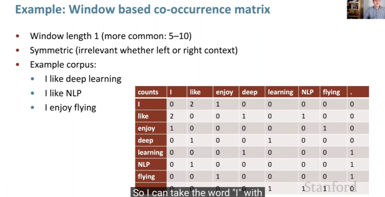
Distributional semantics converts a qualitative linguistic insight into a quantitative modeling strategy. A corpus provides observations of word-context co-occurrence, and an embedding algorithm converts those observations into dense vectors. In traditional count-based approaches, this relationship can be represented using a word-context matrix, where each row corresponds to a word and each column corresponds to a context. Neural embedding methods later replaced explicit sparse count matrices with learned low-dimensional dense representations, but the underlying intuition remained the same: meaning is inferred from contextual behavior.
-
This framework marks an important shift from discrete symbolic representations to continuous knowledge representation. Earlier NLP systems often treated language as a set of discrete units, such as vocabulary items, dictionary entries, or sparse count features. Word embeddings instead represent linguistic knowledge as coordinates in a continuous vector space, where semantic similarity can be modeled through geometry.
-
This is why word embeddings are not arbitrary numerical encodings. They are learned representations shaped by statistical regularities in language. Efficient Estimation of Word Representations in Vector Space by Mikolov et al. (2013) operationalized this idea through predictive objectives such as CBOW and Skip-gram, while GloVe: Global Vectors for Word Representation by Pennington et al. (2014) showed how global co-occurrence statistics could also be used to learn semantically meaningful vectors.
Dense Representations of Words
- Word embeddings, also known as word vectors, provide dense, continuous, and compact representations of words, encoding semantic and syntactic attributes in real-valued vector form. The proximity of vectors in a multidimensional space indicates linguistic relationships between words.
An embedding is a point in an \(N\)-dimensional space, where \(N\) represents the number of dimensions of the embedding.
-
This representation differs sharply from one-hot or sparse count-based encodings. In a one-hot vector, each word is represented as an isolated index, so all words are equally distant from one another. In an embedding space, by contrast, words occupy learned positions, and geometric proximity can reflect semantic similarity, syntactic similarity, topical association, or other learned linguistic regularities.
-
Because embedding vectors are continuous, their coordinates can take many possible real-valued positions rather than fixed binary values. This continuity gives embeddings a degree of representational flexibility: small movements in the space can correspond to gradual changes in meaning, association, register, or domain.
-
This view can be compared to coordinates on a map. Just as latitude and longitude locate places in a two-dimensional geographic space, embedding coordinates locate words in a high-dimensional semantic space. The analogy is imperfect, since embedding dimensions are learned and usually not directly interpretable, but it captures the idea that words become positioned relative to one another through learned relational structure.
-
Formally, a word embedding model learns a mapping:
\[f_\theta : \mathcal{V} \rightarrow \mathbb{R}^d\]-
where \(\mathcal{V}\) is the vocabulary and \(d\) is the embedding dimension. Each word \(w \in \mathcal{V}\) is assigned a vector:
\[e_w = f_\theta(w)\]- where \(e_w \in \mathbb{R}^d\).
-
From Co-Occurrence to Geometry
-
Word embeddings are constructed by learning dense vectors such that words appearing in similar contexts receive similar representations. Each dimension contributes to the representation, but meaning is distributed across the full vector rather than stored in a single coordinate. For example, the concept of “banking” is not localized to one dimension; it is represented by a pattern across many dimensions, capturing associations with finance, deposits, loans, institutions, and related contexts.
-
This distributed representation is central to how embeddings encode meaning. A word’s semantics are not stored as a single symbolic label; instead, they emerge from the interaction of many vector components. This makes embeddings compact, expressive, and suitable for numerical computation.
- The term “embedding” refers to the transformation of discrete words into continuous vectors. These vectors are learned so that they encode a significant portion of a word’s semantic and syntactic behavior. A classic illustration is vector arithmetic:
-
Distributed Representations of Words and Phrases and their Compositionality by Mikolov et al. (2013) demonstrated that learned word vectors can exhibit such regularities, while Linguistic Regularities in Continuous Space Word Representations by Mikolov et al. (2013) studied these analogy-like relationships more directly.
-
The figure below (source) shows distributional vectors represented by a \(D\)-dimensional vector where \(D<<V\), where \(V\) is size of the vocabulary.

Training Word Embeddings
-
Word embeddings are typically pre-trained on large, unlabeled text corpora. Training often involves optimizing auxiliary objectives that require the model to predict a word from its context or predict surrounding context words from a target word. In Word2Vec, the Continuous Bag-of-Words objective predicts a target word from its surrounding context, while the Skip-gram objective predicts surrounding context words from a target word. Efficient Estimation of Word Representations in Vector Space by Mikolov et al. (2013) introduced these efficient predictive architectures.
-
For a target word \(w_t\) and context words \(w_{t-c}, \dots, w_{t+c}\), a simplified Skip-gram objective maximizes:
- Because computing a full softmax over a large vocabulary is expensive, Word2Vec uses approximations such as negative sampling and hierarchical softmax. Word2Vec Explained: Deriving Mikolov et al.’s Negative-Sampling Word-Embedding Method by Goldberg and Levy (2014) provides a mathematical derivation of the negative-sampling objective, and Neural Word Embedding as Implicit Matrix Factorization by Levy and Goldberg (2014) shows that Skip-gram with Negative Sampling implicitly factorizes a shifted PMI matrix.
Similarity and Semantic Comparison
- The effectiveness of word embeddings lies in their ability to capture similarities between words. This is typically measured using cosine similarity:
-
Cosine similarity measures whether two vectors point in similar directions, independent of their magnitude. In embedding spaces, this is useful because semantic relatedness is often reflected more reliably by angular proximity than by raw vector length.
-
These similarity properties make word embeddings useful for search, clustering, classification, analogy evaluation, sentiment analysis, and many other NLP tasks.
Relationship to Traditional NLP Representations
-
Word embeddings emerged partly in response to limitations of earlier sparse representations such as Bag-of-Words, TF-IDF, and manually curated lexical resources. Sparse representations are interpretable and efficient for many retrieval settings, but they do not naturally encode semantic similarity. For example, the words “car” and “automobile” may be treated as unrelated if they appear as distinct vocabulary entries.
-
Dense embeddings address this limitation by learning continuous representations from distributional evidence. Don’t Count, Predict! A Systematic Comparison of Context-Counting vs. Context-Predicting Semantic Vectors by Baroni et al. (2014) compared count-based and predictive semantic vectors, showing the empirical strength of predictive embeddings such as Word2Vec across semantic tasks.
-
Over time, word embeddings became a fundamental layer in neural NLP systems. Although early word embedding models often used relatively shallow neural networks, their learned vectors became foundational inputs for deeper architectures, including recurrent networks, convolutional networks, Transformers, and later contextual encoders.
Limitations of Static Word Embeddings
-
Static word embeddings assign one vector per word type. This means that a polysemous word such as “bank” receives a single representation, even though it may refer to a financial institution or the side of a river. This limitation motivates contextual embeddings, where a word representation depends on surrounding text.
-
For example:
-
Static embeddings approximate an average meaning across contexts, while contextual models compute token representations dynamically. ELMo: Deep Contextualized Word Representations by Peters et al. (2018) introduced deep contextual word representations derived from bidirectional language models, and BERT by Devlin et al. (2018) established Transformer-based bidirectional contextual representations.
-
This transition from static to contextual embeddings generalizes the coordinate-space intuition. Instead of assigning one fixed location to each word type, contextual models compute a different vector depending on the full sentence or document context. For example, “bank” in “river bank” and “bank loan” can occupy different positions in representation space, allowing the model to capture polysemy more accurately.
From Word Embeddings to Contextual Embeddings
-
Contextual embeddings extend the same conceptual framework from isolated word types to token representations that depend on surrounding context. Static word embeddings assign one vector to each word regardless of usage, while contextual embedding models compute different vectors for the same word depending on the sentence, paragraph, or document in which it appears.
-
In models such as ELMo: Deep Contextualized Word Representations by Peters et al. (2018), token representations are produced from bidirectional language models, allowing a word’s vector to change according to its context. BERT by Devlin et al. (2018) further established Transformer-based bidirectional contextual representations, with the base model commonly using 768-dimensional hidden states. Across these systems, an embedding can still be understood as a learned coordinate in a high-dimensional semantic space, but that coordinate is computed dynamically rather than fixed per vocabulary item. A detailed discourse of this embedding technique has been offered in the BERT primer.
-
This transition is especially important for polysemy. For example, the word “bank” should have different representations in “river bank” and “savings bank.” A contextual encoder computes:
-
Phrase-level and entity-level representations also become more context-sensitive under contextual embedding models. A phrase such as “Jennifer Aniston” may be represented differently in contexts about television, film, celebrity news, or biography. If the surrounding text includes “TV series,” the representation may shift toward contexts associated with sitcoms and entertainment rather than toward unrelated uses of the same entity name. This reflects the broader idea that embeddings encode relational structure, but it should not be interpreted as exact symbolic reasoning.
-
Because contextual embeddings are learned from large-scale corpora and rich pretraining objectives, they can capture nuanced associations across syntax, semantics, discourse, and domain. However, this also means they may encode corpus biases, spurious correlations, or unstable associations. Embedding geometry is therefore useful but probabilistic rather than deterministic.
Role of Word Embeddings in Modern NLP
-
Word embeddings efficiently encode semantic and syntactic regularities, making them a central bridge between symbolic language and numerical computation. They also introduced the geometric view of language that later systems extended to sentence embeddings, document embeddings, retrieval embeddings, and multimodal embeddings.
-
Although modern embedding systems often operate at sentence, document, or multimodal levels, word embeddings remain conceptually important because they establish the core idea that meaning can be represented as learned geometry. This idea underlies later systems such as Sentence-BERT by Reimers and Gurevych (2019), SimCSE by Gao et al. (2021), and LLM-derived embedding models.
Related: WordNet
-
WordNet is one of the earliest and most influential attempts to digitally encode lexical meaning in a machine-readable form. WordNet organizes English nouns, verbs, adjectives, and adverbs into synonym sets, or synsets, where each synset corresponds to a lexicalized concept. WordNet: A Lexical Database for English by Miller (1995) describes WordNet as a lexical database designed for programmatic use, with semantic relations linking synonym sets.
-
Unlike a conventional dictionary, WordNet is structured as a semantic network. Words are connected through lexical and conceptual relations, including synonymy, antonymy, hypernymy, hyponymy, meronymy, and entailment. In this structure, a hypernym represents a more general category, while a hyponym represents a more specific instance. For example:
-
This hierarchical structure made WordNet useful for early NLP tasks such as word sense disambiguation, semantic similarity, query expansion, information retrieval, and lexical inference. WordNet: An Electronic Lexical Database by Fellbaum (1998) expanded the resource into a broader account of lexical organization and computational semantics.
-
However, WordNet also illustrates the limitations of manually curated lexical knowledge bases. Its meaning representation is discrete and symbolic: a word sense is represented by membership in a synset and by manually specified relations to other synsets. This makes WordNet interpretable and linguistically precise, but it also limits its coverage of graded similarity, contextual nuance, domain-specific usage, and rapidly changing language. The official WordNet site notes that Princeton WordNet is no longer actively developed, although the database and tools remain freely available.
-
WordNet differs from distributional semantics in an important way. WordNet encodes meaning through explicit lexical relations curated by experts, whereas distributional semantics infers meaning from corpus usage patterns. The distributional hypothesis, introduced in Distributional Structure by Harris (1954), states that words occurring in similar contexts tend to have similar meanings. This principle later became central to word embedding methods.
-
Word embeddings therefore represent a shift from symbolic lexical databases to learned continuous representations. Instead of assigning words to manually curated synsets, embedding models learn vectors from large text corpora:
\[f_\theta : \mathcal{V} \rightarrow \mathbb{R}^d\]- where \(\mathcal{V}\) is the vocabulary and \(d\) is the embedding dimension. In this representation, semantic relatedness is modeled geometrically rather than through explicit graph edges.
-
Similarity between two words can then be computed using cosine similarity:
-
This makes embeddings especially useful for capturing graded semantic relationships. For example, “car” and “automobile” may be close in vector space even if no explicit lexical rule is provided. Efficient Estimation of Word Representations in Vector Space by Mikolov et al. (2013) demonstrated that predictive neural objectives can learn such continuous word vectors efficiently from large corpora.
-
The transition from WordNet to embeddings is therefore not a replacement of one paradigm by another, but a shift in representational emphasis. WordNet provides interpretable symbolic structure, while embeddings provide scalable, data-driven semantic geometry. Modern NLP systems often benefit from both views: lexical resources offer precise relational knowledge, while embeddings support flexible similarity, retrieval, clustering, and generalization across noisy real-world language.
Background: Synonymy, Antonymy, and Polysemy (Multi-Sense)
- Synonymy deals with words that share similar meanings, antonymy concerns words with opposite meanings, and polysemy refers to a single word carrying multiple related meanings. Together, these three relationships form a core part of lexical semantics — the study of meaning in words and their interrelations. They define how language encodes similarity, contrast, and multiplicity of sense, shaping both communication and interpretation.
Synonymy
- Synonymy refers to the linguistic phenomenon where two or more words have the same or very similar meanings. Synonyms are words that can often be used interchangeably in many contexts, although subtle nuances, connotations, or stylistic preferences might make one more appropriate than another in specific situations.
- Synonymy is a vital aspect of language as it provides speakers with a choice of words, adding richness, variety, and flexibility to expression.
Characteristics of Synonymy
-
Complete Synonymy: This is when two words mean exactly the same thing in all contexts, with no differences in usage or connotation. However, true cases of complete synonymy are extremely rare.
- Example: car and automobile.
-
Partial Synonymy: In most cases, synonyms share similar meanings but might differ slightly in terms of usage, formality, or context.
- Example: big and large are generally synonymous but might be preferred in different contexts (e.g., “big mistake” vs. “large building”).
-
Different Nuances: Even if two words are synonyms, one might carry different emotional or stylistic undertones.
- Example: childish vs. childlike. Both relate to behaving like a child, but childish often has a negative connotation, while childlike tends to be more positive.
-
Dialects and Variations: Synonyms can vary between regions or dialects.
- Example: elevator (American English) and lift (British English).
Antonymy
- Antonymy describes the semantic relationship between words that express opposite or contrasting meanings. It is as fundamental to linguistic structure as synonymy because it defines conceptual boundaries and helps organize meaning across dimensions such as quantity, quality, direction, and emotion. Antonyms play an essential role in how humans perceive, categorize, and describe the world, often occurring as natural pairs that emphasize contrast and polarity.
Types of Antonymy
-
Gradable Antonyms: Words that occupy opposite ends of a continuous scale or spectrum.
- Example: hot and cold, happy and sad, tall and short.
- These antonyms allow intermediate degrees (warm, lukewarm, neutral) and can be intensified or diminished using degree modifiers (very cold, quite happy). Importantly, negating one term doesn’t imply the other (not hot ≠ cold).
-
Complementary Antonyms: Pairs where the existence of one necessarily implies the absence of the other — there is no middle ground.
- Example: alive vs. dead, present vs. absent, true vs. false.
- These opposites are binary and mutually exclusive within their conceptual domain.
-
Relational (Conversive) Antonyms: Words that express reciprocal relationships, where one implies the other from a different perspective.
- Example: buy vs. sell, parent vs. child, teacher vs. student.
- The contrast here arises from role reversal rather than direct negation.
-
Directional Antonyms: Words expressing movement or orientation in opposite directions.
- Example: up vs. down, enter vs. exit, rise vs. fall.
Linguistic and Cognitive Role
- Antonymy defines semantic contrast, allowing speakers to express differentiation and opposition, which are crucial to reasoning and classification.
- It contributes to cognitive structuring, framing concepts along continua of meaning and helping categorize experience (e.g., light–dark, good–bad, success–failure).
- In computational linguistics and NLP, antonymy presents a notable challenge: while antonyms are semantically related, they exhibit negative correlation in meaning. Embedding models, which rely on co-occurrence statistics, often mistakenly place antonyms near each other in vector space because they appear in similar syntactic contexts (e.g., hot and cold co-occur with temperature).
- Therefore, distinguishing opposition from similarity remains a crucial goal in developing semantically aware models.
Polysemy (Multi-Sense)
- Polysemy occurs when a single word or expression has multiple related meanings or senses that share a conceptual or historical connection. Unlike homonymy, where words share the same spelling or pronunciation but have entirely unrelated meanings (e.g., bat — the flying mammal vs. bat — the sports implement), polysemy captures how one lexical form can extend its meaning through metaphor, metonymy, or functional association.
Characteristics of Polysemy
-
Multiple Related Meanings: A polysemous word carries several senses that stem from a shared semantic root or conceptual metaphor.
-
Example: Bank can refer to:
- a financial institution (I deposited money in the bank),
- the side of a river (We walked along the river bank).
-
Despite differing domains, both meanings involve the concept of accumulation — of money or land — showing a conceptual link rather than arbitrary coincidence.
-
-
Semantic Extension: New meanings of polysemous words often evolve through metaphorical or functional extensions of an existing sense.
-
Example: Head:
- Literal: part of the human body (She nodded her head),
- Metaphorical: leader of a group (the head of the company),
- Functional: the front or top of something (the head of the line).
-
Each new sense maintains a logical or spatial connection to the core concept of top or control.
-
-
Context-Dependent Interpretation: The correct sense of a polysemous word depends on the context in which it appears.
-
Example: Run:
- Movement (She runs every morning),
- Operation (The engine runs smoothly),
- Management (He runs the business).
-
The surrounding words and syntax determine which sense is activated.
-
-
Cognitive Efficiency: Polysemy demonstrates the economy of language, where existing lexical forms are reused for conceptually related meanings rather than inventing new words for every nuance. This flexibility enhances communication while minimizing vocabulary load.
Linguistic and Computational Relevance
- In linguistics, polysemy illustrates how meaning evolves through metaphor, metonymy, and conceptual mapping, making it central to studies of semantic change.
- In computational linguistics and NLP, polysemy introduces word sense ambiguity — a major challenge in embedding and translation models. Traditional word embeddings like Word2Vec assign one vector per word, merging multiple senses (e.g., bank as finance and geography), while contextual models like BERT dynamically adjust meaning based on context, successfully distinguishing different senses of the same word.
Key Differences Between Synonymy, Antonymy, and Polysemy
-
Synonymy involves different words that have similar or identical meanings.
- Example: happy and joyful both convey the sense of positive emotion, differing mainly in tone or intensity.
- Synonyms often cluster around the same semantic field, allowing subtle variation in expression without changing the fundamental meaning.
-
Antonymy involves different words that express opposite or contrasting meanings.
- Example: increase vs. decrease, love vs. hate.
- Unlike synonyms, antonyms establish a semantic axis of contrast, defining boundaries of meaning (e.g., hot–cold, true–false). This contrast helps structure conceptual domains in a way that allows gradation and polarity.
-
Polysemy involves a single word that carries multiple related meanings.
- Example: bright can mean intelligent or full of light.
- Polysemy reflects the dynamic evolution of meaning, showing how words adapt across contexts while maintaining a conceptual link between senses.
Comparative Analysis
| Aspect | Synonymy | Antonymy | Polysemy |
|---|---|---|---|
| Number of Words | Two or more different words | Two or more different words | One word with multiple meanings |
| Meaning Relationship | Similar or identical | Opposite or contrasting | Related but distinct |
| Example | begin / start | light / dark | paper (material / essay) |
| Function in Language | Adds expressiveness and variety | Defines contrast and logical opposition | Enables flexibility and metaphorical extension |
| Challenge in NLP | Identifying subtle contextual preference | Detecting oppositional relations despite similar contexts | Distinguishing multiple senses in one vector representation |
- In summary, synonymy enriches language through variation, antonymy structures meaning through opposition, and polysemy fuels adaptability and semantic evolution. Together, they define the intricate web of relationships that make natural language both expressive and conceptually organized.
Why Are Synonymy, Antonymy, and Polysemy Important?
- Synonymy enriches language by giving speakers multiple ways to express the same concept, allowing for stylistic variation, precision, and emotional nuance. It underpins paraphrasing, synonym substitution, and diversity in expression.
- Antonymy provides the structural backbone of contrast in meaning, enabling logical reasoning, polarity, and comparison. It helps define categorical boundaries (e.g., good vs. bad, success vs. failure) and sharpens conceptual distinctions in discourse.
-
Polysemy reflects the evolutionary adaptability of language. Words develop multiple meanings over time through metaphorical, cultural, or functional extensions, allowing speakers to describe new ideas without constantly coining new terms.
- Together, these three relationships create the semantic topology of language — the intricate network through which meaning is differentiated, extended, and interconnected.
Challenges
-
Ambiguity: Synonymy, antonymy, and polysemy all introduce potential ambiguity in communication.
- For instance, polysemy can obscure meaning (She banked by the river — financial or geographic sense?), while antonymy can lead to subtle contextual inversions (not happy doesn’t necessarily mean sad).
-
Disambiguation in Language Processing: In linguistics and natural language processing (NLP), determining whether two words are similar (synonyms), opposite (antonyms), or multi-sense (polysemous) remains a central challenge.
- Word embeddings like Word2Vec often capture relatedness rather than true semantic opposition, leading antonyms (hot, cold) to appear close in vector space.
- Contextual models such as BERT address polysemy by dynamically adjusting word meaning based on surrounding text, but fine-grained semantic disambiguation — distinguishing similarity from contrast — remains an open area of research in computational semantics.
Word Embedding Techniques
- Accurately representing the meaning of words is a crucial aspect of NLP. This task has evolved significantly over time, with various techniques being developed to capture the nuances of word semantics.
- Count-based methods like TF-IDF and BM25 focus on word frequency and document uniqueness, offering basic information retrieval capabilities.
- Co-occurrence-based techniques such as Word2Vec, GloVe, and fastText analyze word contexts in large corpora, capturing semantic relationships and morphological details.
- Contextualized models like BERT and ELMo provide dynamic, context-sensitive embeddings, significantly enhancing language understanding by generating varied representations for words based on their usage in sentences.
-
The details of this taxonomy are as follows:
- Count-Based Techniques (TF-IDF and BM25):
- These methods, originating in information retrieval, rely on counting word occurrences within and across documents.
- TF-IDF identifies words that are frequent in a document but rare in the corpus, emphasizing their discriminative power.
- BM25 improves upon TF-IDF through probabilistic modeling, incorporating document length normalization and term saturation.
- While effective for keyword-based retrieval, these approaches are not semantic—they treat words as independent symbols without capturing meaning or contextual relationships.
- Co-occurrence Based / Static Embedding Techniques (Word2Vec, GloVe, fastText):
- These models mark the transition from frequency-based to predictive and semantic approaches.
- Word2Vec learns embeddings by predicting context words from a target (Skip-gram) or vice versa (CBOW), yielding dense vector representations that reflect semantic similarity.
- GloVe (Global Vectors for Word Representation) combines global co-occurrence statistics with local context learning, encoding both syntactic and semantic regularities.
- fastText extends Word2Vec by incorporating subword information, enabling the model to represent morphological variations and unseen words.
- These embeddings are static—each word has a single vector—but they are inherently semantic, as vector distances correspond to meaning-based similarity.
-
Contextualized / Dynamic Representation Techniques (ELMo, BERT):
- ELMo (Embeddings from Language Models) generates context-dependent embeddings by processing text bidirectionally using deep recurrent neural networks, allowing the same word to have different representations depending on its sentence context.
- BERT (Bidirectional Encoder Representations from Transformers) advances this idea using Transformer architecture, encoding bidirectional dependencies and enabling fine-grained understanding of syntax, semantics, and ambiguity.
- These models produce dynamic semantic embeddings—vectors that adapt to context, capturing multiple senses (polysemy) and resolving ambiguity more effectively than static models.
- Count-Based Techniques (TF-IDF and BM25):
Semantic Similarity and its Geometric Interpretation
-
In the process of learning representations, the models that produce semantic embeddings—namely Word2Vec, GloVe, fastText, BERT, and ELMo—map words into a geometric space such that semantic similarity corresponds to geometric (spatial) proximity in the embedding space. Words that occur in similar linguistic environments cluster together, allowing computational models to reason about meaning quantitatively and perform tasks such as analogy, clustering, and semantic search with human-like sensitivity to contextual meaning. Put simply, in these vector spaces, words with similar meanings or functions occupy nearby regions, and the degree of similarity is measured using geometric metrics such as cosine similarity, dot product, or Euclidean distance.
-
This geometric perspective enables embeddings to encode linguistic relationships as spatial relationships:
- Synonyms (e.g., king, monarch) lie close to each other because they occur in similar contexts.
- Analogical relationships (e.g., man : woman :: king : queen) manifest through vector arithmetic, where semantic relations correspond to geometric offsets.
- Antonyms (e.g., hot, cold) may also appear close due to shared contextual environments, highlighting a limitation of distributional methods that capture relatedness rather than true opposition.
Bag of Words (BoW)
Concept
- Bag of Words (BoW) is a simple and widely used technique for text representation in NLP. It represents text data (documents) as vectors of word counts, disregarding grammar and word order but keeping multiplicity. Each unique word in the corpus is a feature, and the value of each feature is the count of occurrences of the word in the document.
Steps to Create BoW Embeddings
- Tokenization:
- Split the text into words (tokens).
- Vocabulary Building:
- Create a vocabulary list of all unique words in the corpus.
- Vector Representation:
- For each document, create a vector where each element corresponds to a word in the vocabulary. The value is the count of occurrences of that word in the document.
Example
- Consider a corpus with the following two documents:
- “The cat sat on the mat.”
- “The dog sat on the log.”
-
Steps:
- Tokenization:
- Document 1:
["the", "cat", "sat", "on", "the", "mat"] - Document 2:
["the", "dog", "sat", "on", "the", "log"]
- Document 1:
- Vocabulary Building:
- Vocabulary:
["the", "cat", "sat", "on", "mat", "dog", "log"]
- Vocabulary:
- Vector Representation:
- Document 1:
[2, 1, 1, 1, 1, 0, 0] - Document 2:
[2, 0, 1, 1, 0, 1, 1]
- Document 1:
- The resulting BoW vectors are:
- Document 1:
[2, 1, 1, 1, 1, 0, 0] - Document 2:
[2, 0, 1, 1, 0, 1, 1]
- Document 1:
- Tokenization:
Limitations of BoW
- Bag of Words (BoW) embeddings, despite their simplicity and effectiveness in some applications, have several significant limitations. These limitations can impact the performance and applicability of BoW in more complex NLP tasks. Here’s a detailed explanation of these limitations:
Lack of Contextual Information
- Word Order Ignored:
- BoW embeddings do not take into account the order of words in a document. This means that “cat sat on the mat” and “mat sat on the cat” will have the same BoW representation, despite having different meanings.
- Loss of Syntax and Semantics:
- The embedding does not capture syntactic and semantic relationships between words. For instance, “bank” in the context of a financial institution and “bank” in the context of a riverbank will have the same representation.
High Dimensionality
- Large Vocabulary Size:
- The dimensionality of BoW vectors is equal to the number of unique words in the corpus, which can be extremely large. This leads to very high-dimensional vectors, resulting in increased computational cost and memory usage.
- Sparsity:
- Most documents use only a small fraction of the total vocabulary, resulting in sparse vectors with many zero values. This sparsity can make storage and computation inefficient.
Lack of Handling of Polysemy and Synonymy
- Polysemy:
- Polysemous words (same word with multiple meanings) are treated as a single feature, failing to capture their different senses based on context. Traditional word embedding algorithms assign a distinct vector to each word, which makes them unable to account for polysemy. For instance, the English word “bank” translates to two different words in French—”banque” (financial institution) and “banc” (riverbank)—capturing its distinct meanings.
- Synonymy:
- Synonyms (different words with similar meaning) are treated as completely unrelated features. For example, “happy” and “joyful” will have different vector representations even though they have similar meanings.
Fixed Vocabulary
- OOV (Out-of-Vocabulary) Words: BoW cannot handle words that were not present in the training corpus. Any new word encountered will be ignored or misrepresented, leading to potential loss of information.
Feature Independence Assumption
- No Inter-Feature Relationships: BoW assumes that the presence or absence of a word in a document is independent of other words. This independence assumption ignores any potential relationships or dependencies between words, which can be crucial for understanding context and meaning.
Scalability Issues
- Computational Inefficiency: As the size of the corpus increases, the vocabulary size also increases, leading to scalability issues. High-dimensional vectors require more computational resources for processing, storing, and analyzing the data.
No Weighting Mechanism
- Equal Importance: In its simplest form, BoW treats all words with equal importance, which is not always appropriate. Common but less informative words (e.g., “the”, “is”) are treated the same as more informative words (e.g., “cat”, “bank”).
Lack of Generalization
- Poor Performance on Short Texts: BoW can be particularly ineffective for short texts or documents with limited content, where the lack of context and the sparse nature of the vector representation can lead to poor performance.
Examples of Limitations
- Example of Lack of Contextual Information:
- Consider two sentences: “Apple is looking at buying a U.K. startup.” and “Startup is looking at buying an Apple.” Both would have similar BoW representations but convey different meanings.
- Example of High Dimensionality and Sparsity:
- A corpus with 100,000 unique words results in BoW vectors of dimension 100,000, most of which would be zeros for any given document.
Summary
- While BoW embeddings provide a straightforward and intuitive way to represent text data, their limitations make them less suitable for complex NLP tasks that require understanding context, handling large vocabularies efficiently, or dealing with semantic and syntactic nuances. More advanced techniques like TF-IDF, word embeddings (e.g., Word2Vec, GloVe, fastText), and contextual embeddings (e.g., ELMo, BERT) address many of these limitations by incorporating context, reducing dimensionality, and capturing richer semantic information.
Term Frequency-Inverse Document Frequency (TF-IDF)
- Term Frequency-Inverse Document Frequency (TF-IDF) is a statistical measure used to evaluate the importance of a word to a document in a collection or corpus. It is a fundamental technique in text processing that ranks the relevance of documents to a specific query, commonly applied in tasks such as document classification, search engine ranking, information retrieval, and text mining.
- The TF-IDF value increases proportionally with the number of times a word appears in the document, but this is offset by the frequency of the word in the corpus, which helps to control for the fact that some words (e.g., “the”, “is”, “and”) are generally more common than others.
Term Frequency (TF)
- Term Frequency measures how frequently a term occurs in a document. Since every document is different in length, it is possible that a term would appear much more times in long documents than shorter ones. Thus, the term frequency is often divided by the document length (the total number of terms in the document) as a way of normalization:
Inverse Document Frequency (IDF)
- Inverse Document Frequency measures how important a term is. While computing TF, all terms are considered equally important. However, certain terms, like “is”, “of”, and “that”, may appear a lot of times but have little importance. Thus, we need to weigh down the frequent terms while scaling up the rare ones, by computing the following:
Example
Steps to Calculate TF-IDF
- Step 1: TF (Term Frequency): Number of times a word appears in a document divided by the total number of words in that document.
- Step 2: IDF (Inverse Document Frequency): Calculated as
log(N / df), where:Nis the total number of documents in the collection.dfis the number of documents containing the word.
- Step 3: TF-IDF: The product of TF and IDF.
Document Collection
- Doc 1: “The sky is blue.”
- Doc 2: “The sun is bright.”
- Total documents (
N): 2
Calculate Term Frequency (TF)
| Word | TF in Doc 1 ("The sky is blue") | TF in Doc 2 ("The sun is bright") |
|---|---|---|
| the | 1/4 | 1/5 |
| sky | 1/4 | 0/5 |
| is | 1/4 | 1/5 |
| blue | 1/4 | 0/5 |
| sun | 0/4 | 1/5 |
| bright | 0/4 | 1/5 |
Calculate Document Frequency (DF) and Inverse Document Frequency (IDF)
| Word | DF (in how many docs) | IDF (log(N/DF)) |
|---|---|---|
| the | 2 | log(2/2) = 0 |
| sky | 1 | log(2/1) ≈ 0.693 |
| is | 2 | log(2/2) = 0 |
| blue | 1 | log(2/1) ≈ 0.693 |
| sun | 1 | log(2/1) ≈ 0.693 |
| bright | 1 | log(2/1) ≈ 0.693 |
Calculate TF-IDF for Each Word
| Word | TF in Doc 1 | IDF | TF-IDF in Doc 1 | TF in Doc 2 | IDF | TF-IDF in Doc 2 |
|---|---|---|---|---|---|---|
| the | 1/4 | 0 | 0 | 1/5 | 0 | 0 |
| sky | 1/4 | log(2) ≈ 0.693 | (1/4) * 0.693 ≈ 0.173 | 0/5 | log(2) ≈ 0.693 | 0 |
| is | 1/4 | 0 | 0 | 1/5 | 0 | 0 |
| blue | 1/4 | log(2) ≈ 0.693 | (1/4) * 0.693 ≈ 0.173 | 0/5 | log(2) ≈ 0.693 | 0 |
| sun | 0/4 | log(2) ≈ 0.693 | 0 | 1/5 | log(2) ≈ 0.693 | (1/5) * 0.693 ≈ 0.139 |
| bright | 0/4 | log(2) ≈ 0.693 | 0 | 1/5 | log(2) ≈ 0.693 | (1/5) * 0.693 ≈ 0.139 |
Explanation of Table
- The TF column shows the term frequency for each word in each document.
- The IDF column shows the inverse document frequency for each word.
- The TF-IDF columns for Doc 1 and Doc 2 show the final TF-IDF score for each word, calculated as
TF * IDF.
Key Observations
- Words like “the” and “is” have an IDF of 0 because they appear in both documents, making them less distinctive.
- Words like “blue,” “sun,” and “bright” have higher TF-IDF values because they appear in only one document, making them more distinctive for that document.
- The TF-IDF score for “blue” in Doc 1 is thus a measure of its importance in that document, within the context of the given document collection. This score would be different in a different document or a different collection, reflecting the term’s varying importance.
Limitations of TF-IDF
- While TF-IDF is a powerful tool for certain applications, the limitations highlighted below make it less suitable for tasks that require deep understanding of language, such as semantic search, word sense disambiguation, or processing of very short or dynamically changing texts. This has led to the development and adoption of more advanced techniques like word embeddings and neural network-based models in NLP.
Lack of Context and Word Order
- TF-IDF treats each word in a document independently and does not consider the context in which a word appears. This means it cannot capture the meaning of words based on their surrounding words or the overall semantic structure of the text. The word order is also ignored, which can be crucial in understanding the meaning of a sentence.
Does Not Account for Polysemy
- Words with multiple meanings (polysemy) are treated the same regardless of their context. For example, the word “bank” would have the same representation in “river bank” and “savings bank”, even though it has different meanings in these contexts.
Lack of Semantic Understanding
- TF-IDF relies purely on the statistical occurrence of words in documents, which means it lacks any understanding of the semantics of the words. It cannot capture synonyms or related terms unless they appear in similar documents within the corpus.
Bias Towards Rare Terms
- While the IDF component of TF-IDF aims to balance the frequency of terms, it can sometimes overly emphasize rare terms. This might lead to overvaluing words that appear infrequently but are not necessarily more relevant or important in the context of the document.
Vocabulary Limitation
- The TF-IDF model is limited to the vocabulary of the corpus it was trained on. It cannot handle new words that were not in the training corpus, making it less effective for dynamic content or languages that evolve rapidly.
Normalization Issues
- The normalization process in TF-IDF (e.g., dividing by the total number of words in a document) may not always be effective in balancing document lengths and word frequencies, potentially leading to skewed results.
Requires a Large and Representative Corpus
- For the IDF part of TF-IDF to be effective, it needs a large and representative corpus. If the corpus is not representative of the language or the domain of interest, the IDF scores may not accurately reflect the importance of the words.
No Distinction Between Different Types of Documents
- TF-IDF treats all documents in the corpus equally, without considering the type or quality of the documents. This means that all sources are considered equally authoritative, which may not be the case.
Poor Performance with Short Texts
- In very short documents, like tweets or SMS messages, the TF-IDF scores can be less meaningful because of the limited word occurrence and context.
Best Match 25 (BM25)
- BM25 is a ranking function used in information retrieval systems, particularly in search engines, to rank documents based on their relevance to a given search query. It’s a part of the family of probabilistic information retrieval models and is an extension of the TF-IDF (Term Frequency-Inverse Document Frequency) approach, though it introduces several improvements and modifications.
Key Components of BM25
-
Term Frequency (TF): BM25 modifies the term frequency component of TF-IDF to address the issue of term saturation. In TF-IDF, the more frequently a term appears in a document, the more it is considered relevant. However, this can lead to a problem where beyond a certain point, additional occurrences of a term don’t really indicate more relevance. BM25 addresses this by using a logarithmic scale for term frequency, which allows for a point of diminishing returns, preventing a term’s frequency from having an unbounded impact on the document’s relevance.
-
Inverse Document Frequency (IDF): Like TF-IDF, BM25 includes an IDF component, which helps to weight a term’s importance based on how rare or common it is across all documents. The idea is that terms that appear in many documents are less informative than those that appear in fewer documents.
-
Document Length Normalization: BM25 introduces a sophisticated way of handling document length. Unlike TF-IDF, which may unfairly penalize longer documents, BM25 normalizes for length in a more balanced manner, reducing the impact of document length on the calculation of relevance.
-
Tunable Parameters: BM25 includes parameters like \(k1\) and \(b\), which can be adjusted to optimize performance for specific datasets and needs. \(k1\) controls how quickly an increase in term frequency leads to term saturation, and \(b\) controls the degree of length normalization.
Example
-
Imagine you have a collection of documents and a user searches for “solar energy advantages”.
- Document A is 300 words long and mentions “solar energy” 4 times and “advantages” 3 times.
- Document B is 1000 words long and mentions “solar energy” 10 times and “advantages” 1 time.
- Using BM25:
- Term Frequency: The term “solar energy” appears more times in Document B, but due to term saturation, the additional occurrences don’t contribute as much to its relevance score as the first few mentions.
- Inverse Document Frequency: If “solar energy” and “advantages” are relatively rare in the overall document set, their appearances in these documents increase the relevance score more significantly.
- Document Length Normalization: Although Document B is longer, BM25’s length normalization ensures that it’s not unduly penalized simply for having more words. The relevance of the terms is balanced against the length of the document.
- So, despite Document B having more mentions of “solar energy”, BM25 will calculate the relevance of both documents in a way that balances term frequency, term rarity, and document length, potentially ranking them differently based on how these factors interplay. The final relevance scores would then determine their ranking in the search results for the query “solar energy advantages”.
BM25: Evolution of TF-IDF
- BM25 is a ranking function used by search engines to estimate the relevance of documents to a given search query. It’s part of the probabilistic information retrieval model and is considered an evolution of the TF-IDF (Term Frequency-Inverse Document Frequency) model. Both are used to rank documents based on their relevance to a query, but they differ in how they calculate this relevance.
BM25
- Term Frequency Component: Like TF-IDF, BM25 considers the frequency of the query term in a document. However, it adds a saturation point to prevent a term’s frequency from disproportionately influencing the document’s relevance.
- Length Normalization: BM25 adjusts for the length of the document, penalizing longer documents less harshly than TF-IDF.
- Tuning Parameters: It includes two parameters, \(k1\) and \(b\), which control term saturation and length normalization, respectively. These can be tuned to suit specific types of documents or queries.
TF-IDF
- Term Frequency: TF-IDF measures the frequency of a term in a document. The more times the term appears, the higher the score.
- Inverse Document Frequency: This component reduces the weight of terms that appear in many documents across the corpus, assuming they are less informative.
- Simpler Model: TF-IDF is generally simpler than BM25 and doesn’t involve parameters like \(k1\) or \(b\).
Example
-
Imagine a search query “chocolate cake recipe” and two documents:
- Document A: 100 words, “chocolate cake recipe” appears 10 times.
- Document B: 1000 words, “chocolate cake recipe” appears 15 times.
Using TF-IDF:
- The term frequency for “chocolate cake recipe” would be higher in Document A.
- Document B, being longer, might get a lower relevance score due to less frequency of the term.
Using BM25:
- The term frequency component would reach a saturation point, meaning after a certain frequency, additional occurrences of “chocolate cake recipe” contribute less to the score.
- Length normalization in BM25 would not penalize Document B as heavily as TF-IDF, considering its length.
- The tuning parameters \(k1\) and \(b\) could be adjusted to optimize the balance between term frequency and document length.
-
In essence, while both models aim to determine the relevance of documents to a query, BM25 offers a more nuanced and adjustable approach, especially beneficial in handling longer documents and ensuring that term frequency doesn’t disproportionately affect relevance.
Limitations of BM25
- Understanding the limitations below is crucial when implementing BM25 in a search engine or information retrieval system, as it helps in identifying cases where BM25 might need to be supplemented with other techniques or algorithms for better performance.
Parameter Sensitivity
- BM25 includes parameters like \(k1\) and \(b\), which need to be fine-tuned for optimal performance. This tuning process can be complex and is highly dependent on the specific nature of the document collection and queries. Inappropriate parameter settings can lead to suboptimal results.
Non-Handling of Semantic Similarities
- BM25 primarily relies on exact keyword matching. It does not account for the semantic relationships between words. For instance, it would not recognize “automobile” and “car” as related terms unless explicitly programmed to do so. This limitation makes BM25 less effective in understanding the context or capturing the nuances of language.
Ineffectiveness with Short Queries or Documents
- BM25’s effectiveness can decrease with very short queries or documents, as there are fewer words to analyze, making it harder to distinguish relevant documents from irrelevant ones.
Length Normalization Challenges
- While BM25’s length normalization aims to prevent longer documents from being unfairly penalized, it can sometimes lead to the opposite problem, where shorter documents are unduly favored. The balance is not always perfect, and the effectiveness of the normalization can vary based on the dataset.
Query Term Independence
- BM25 assumes independence between query terms. It doesn’t consider the possibility that the presence of certain terms together might change the relevance of a document compared to the presence of those terms individually.
Difficulty with Rare Terms
- Like TF-IDF, BM25 can struggle with very rare terms. If a term appears in very few documents, its IDF (Inverse Document Frequency) component can become disproportionately high, skewing results.
Performance in Specialized Domains
- In specialized domains with unique linguistic features (like legal, medical, or technical fields), BM25 might require significant customization to perform well. This is because standard parameter settings and term-weighting mechanisms may not align well with the unique characteristics of these specialized texts.
Ignoring Document Quality
- BM25 focuses on term frequency and document length but doesn’t consider other aspects that might indicate document quality, such as authoritativeness, readability, or the freshness of information.
Vulnerability to Keyword Stuffing
- Like many other keyword-based algorithms, BM25 can be susceptible to keyword stuffing, where documents are artificially loaded with keywords to boost relevance.
Incompatibility with Complex Queries
- BM25 is less effective for complex queries, such as those involving natural language questions or multi-faceted information needs. It is designed for keyword-based queries and may not perform well with queries that require understanding of context or intent.
Word2Vec
- Proposed in Efficient Estimation of Word Representations in Vector Space by Mikolov et al. (2013), the Word2Vec algorithm marked a significant advancement in the field of NLP as a notable example of a word embedding technique.
- Word2Vec is renowned for its effectiveness in learning word vectors, which are then used to decode the semantic relationships between words. It utilizes a vector space model to encapsulate words in a manner that captures both semantic and syntactic relationships. This method enables the algorithm to discern similarities and differences between words, as well as to identify analogous relationships, such as the parallel between “Stockholm” and “Sweden” and “Cairo” and “Egypt.”
- Word2Vec’s methodology of representing words as vectors in a semantic and syntactic space has profoundly impacted the field of NLP, offering a robust framework for capturing the intricacies of language and its usage.
Motivation
- Word2Vec introduced a fundamental shift in NLP by allowing efficient learning of distributed word representations that capture both semantic and syntactic relationships.
- These embeddings support a wide range of downstream tasks, such as text classification, translation, and recommendation systems, due to their ability to encode meaning in vector space.
- Key advantages include:
- The ability to capture semantic similarity — words appearing in similar contexts have similar vector representations.
- Support for vector arithmetic to reveal analogical relationships (for example, “king - man + woman ≈ queen”).
- Computational efficiency due to simplified training strategies such as negative sampling and hierarchical softmax (covered in detail later).
- A shallow network design, allowing rapid training even on large corpora.
- Generalization across linguistic tasks by representing words in a continuous vector space rather than as discrete symbols.
Theoretical Foundation: Distributional Hypothesis
-
At the heart of Word2Vec lies the distributional hypothesis in linguistics, which states that “words that occur in similar contexts tend to have similar meanings.” Formally, this implies that the meaning of a word \(w\) can be inferred from the statistical distribution of other words that co-occur with it in text.
-
If \(C(w)\) denotes the set of context words appearing around \(w\) within a fixed window, Word2Vec seeks to learn an embedding function \(f: w \mapsto v_w \in \mathbb{R}^N\) that maximizes the likelihood of observing those context words.
-
Thus, for every word \(w_t\) in the corpus, the training objective is to maximize:
\[\frac{1}{T} \sum_{t=1}^{T} \sum_{-c \le j \le c, j \ne 0} \log p(w_{t+j} | w_t)\]- where \(c\) is the context window size and \(T\) is the corpus length.
Representational Power and Semantic Arithmetic
- One of the key insights from Word2Vec is that semantic relationships between words can be captured through linear relationships in vector space. This means that algebraic operations on word vectors can reveal linguistic regularities, such as:
- These relationships emerge naturally because Word2Vec embeds words in such a way that cosine similarity corresponds to semantic relatedness:
- This property allows for analogical reasoning, clustering, and downstream use in a wide range of NLP tasks.
Probabilistic Interpretation
-
From a probabilistic standpoint, Word2Vec models the conditional distribution of context words given a target word (Skip-gram) or a target word given its context (CBOW). The softmax function formalizes this as:
\[p(w_o | w_i) = \frac{\exp(u_{w_o}^T v_{w_i})}{\sum_{w' \in V} \exp(u_{w'}^T v_{w_i})}\]-
where
- \(v_{w_i}\) is the input vector (representing the center or target word),
- \(u_{w_o}\) is the output vector (representing the context word), and
- \(V\) is the vocabulary.
-
-
This formulation defines a differentiable objective that allows embeddings to be learned through backpropagation and stochastic gradient descent.
-
The following figure (source) shows a simplified visualization of the training process using context prediction.
Motivation behind Word2Vec: The Need for Context-based Semantic Understanding
- Traditional approaches to textual representation—such as TF-IDF and BM25—treat words as independent entities and rely on counting-based statistics rather than semantic relationships. While these methods are effective for ranking documents or identifying keyword importance, they fail to represent the contextual and relational meaning that underpins natural language.
- The motivation for Word2Vec arises from the limitations of count-based models that fail to capture semantics. By introducing a predictive, context-driven learning mechanism, Word2Vec constructs a semantic embedding space where contextual relationships between words are preserved. This makes it a foundational technique for subsequent deep learning models such as GloVe by Pennington et al. (2014), fastText by Bojanowski et al. (2017), ELMo by Peters et al. (2018), and BERT by Devlin et al. (2018), which further refine contextual understanding at the sentence and discourse level.
Background: Limitations of Frequency-based Representations
-
TF-IDF (Term Frequency–Inverse Document Frequency):
-
This method assigns weights to terms based on how frequently they appear in a document and how rare they are across a corpus.
-
Mathematically, the weight for a term \(t\) in a document \(d\) is given by:
\[\text{TF-IDF}(t, d) = \text{TF}(t, d) \times \log\frac{N}{\text{DF}(t)}\]- where \(\text{TF}(t, d)\) is the frequency of term \(t\) in document \(d\), \(\text{DF}(t)\) is the number of documents containing \(t\), and \(N\) is the total number of documents.
-
While TF-IDF captures word importance, it ignores semantic similarity—two words like “doctor” and “physician” are treated as entirely distinct, even though they share similar meanings.
-
-
BM25 (Best Matching 25):
-
BM25 is a probabilistic ranking function often used in information retrieval, first described by Robertson & Walker (1994). It improves upon TF-IDF by introducing parameters to handle term saturation and document length normalization:
\[\text{BM25}(t, d) = \log\left(\frac{N - \text{DF}(t) + 0.5}{\text{DF}(t) + 0.5}\right) \cdot \frac{(k_1 + 1) \text{TF}(t, d)}{k_1 \left[(1 - b) + b\frac{|d|}{\text{avgdl}}\right] + \text{TF}(t, d)}\]- where \(k_1\) and \(b\) are tunable parameters, \(\mid d \mid\) is the document length, and \(\text{avgdl}\) is the average document length across the corpus.
-
BM25 effectively balances term relevance and document length normalization, but it remains a lexical rather than semantic measure. It doesn’t model relationships such as synonymy, antonymy, or analogy.
-
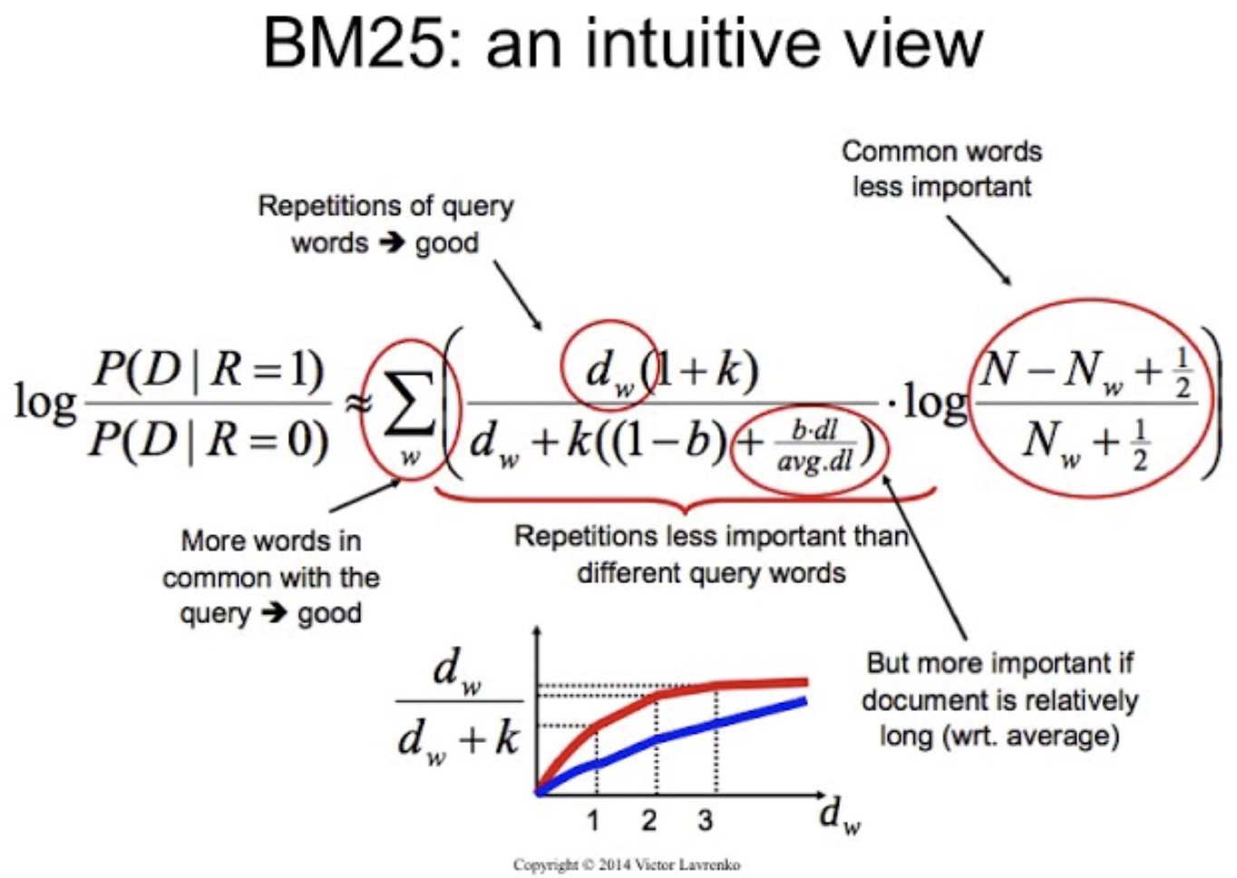
The figure below (source) provides an intuitive visualization of the BM25 mechanism. It shows how the formula rewards documents containing more query word repetitions (up to a saturation point) while discounting overly common terms. The right-hand logarithmic component reduces the weight of frequent words, while the normalization term adjusts for document length. The graph below the equation illustrates how term frequency contributions flatten as occurrences increase, reflecting diminishing returns for repeated terms.
-
Motivation for Contextual Representations
-
Human language is inherently contextual: the meaning of a word depends on the words surrounding it. For example, the word bank in “river bank” differs from bank in “bank loan.”
- Frequency-based methods cannot distinguish these meanings because they represent bank as a single static token.
- What is required is a context-aware model that learns word meaning from its usage patterns in sentences—capturing semantics not just by frequency, but by co-occurrence structure and distributional behavior.
Word2Vec as a Contextual Solution
- Word2Vec resolves these shortcomings by learning dense, low-dimensional embeddings that encode semantic similarity through co-occurrence patterns.
- Instead of treating each word as an independent unit, Word2Vec models conditional probabilities such as:
- These probabilities are parameterized by neural network weights that correspond to word embeddings.
- Through training, the model positions semantically similar words near each other in the embedding space.
Semantic Vector Space: A Conceptual Leap
- In Word2Vec, each word is represented as a continuous vector \(v_w \in \mathbb{R}^N\), where semantic similarity corresponds to geometric proximity.
-
This vector representation allows the model to capture linguistic phenomena that statistical models cannot:
- Synonymy: Words like “car” and “automobile” appear near each other.
- Antonymy: Words like “hot” and “cold” occupy positions with structured contrastive relations.
- Analogies: Relationships such as \(v_{\text{Paris}} - v_{\text{France}} + v_{\text{Italy}} \approx v_{\text{Rome}}\) demonstrate how linear vector operations encode relational meaning.
Comparison with Traditional Models
| Aspect | TF-IDF | BM25 | Word2Vec |
|---|---|---|---|
| Representation | Sparse, count-based | Sparse, probabilistic | Dense, continuous |
| Captures context | No | No | Yes |
| Semantic similarity | Not modeled | Not modeled | Explicitly modeled |
| Handles polysemy | No | No | Partially (through contextual learning but not fully since it assigns a single vector per word) |
| Learning mechanism | Frequency-based | Probabilistic ranking | Neural prediction |
Why Context Matters: Intuitive Illustration
- Imagine reading the sentence: “The bat flew across the cave.”, and then another: “He swung the bat at the ball.”
- In traditional models, the token “bat” is identical in both contexts.
- However, Word2Vec distinguishes them by how “bat” co-occurs with words like flew, cave, swung, and ball. The embeddings for these contexts push the representation of bat toward two distinct regions of the semantic space—one near animals, the other near sports equipment.
Core Idea
- Word2Vec represents a transformative shift in natural language understanding by learning word meanings through prediction tasks rather than through counting word co-occurrences.
- At its core, the algorithm employs a shallow neural network trained on a large corpus to predict contextual relationships between words, producing dense, meaningful vector representations that encode both syntactic and semantic regularities.
- The core idea behind Word2Vec is to transform linguistic co-occurrence information into a geometric form that captures word meaning through spatial relationships. It does this not by memorizing frequencies, but by predicting contexts, allowing the embedding space to inherently encode semantic similarity, analogy, and syntactic relationships in a mathematically continuous manner.
Predictive Nature of Word2Vec
-
Unlike earlier statistical methods that rely on co-occurrence counts (e.g., Latent Semantic Analysis by Deerwester et al. (1990)), Word2Vec learns embeddings by solving a prediction problem:
- Given a target word, predict its context words (Skip-gram).
- Given a set of context words, predict the target word (CBOW).
-
This approach stems from the distributional hypothesis, operationalized via probabilistic modeling.
-
Formally, for a corpus with words \(w_1, w_2, \dots, w_T\), and context window size \(c\), the model maximizes the following average log probability:
- This objective encourages the model to learn embeddings \(v_{w_t}\) and \(u_{w_{t+j}}\) such that similar words (those that appear in similar contexts) have similar vector representations.
Word Vectors and Semantic Encoding
-
Each word \(w\) in the vocabulary is associated with two vectors:
- Input vector \(v_w\): representing the word when it is the center (target) word.
- Output vector \(u_w\): representing the word when it appears in the context.
-
These vectors are columns in the weight matrices:
- \(W \in \mathbb{R}^{V \times N}\) (input-to-hidden layer)
- \(W' \in \mathbb{R}^{N \times V}\) (hidden-to-output layer)
-
Thus, the total parameters of the model are \(\theta = {W, W'}\), and for any word \(w_i\) and context word \(c\):
\[p(w_i | c) = \frac{\exp(u_{w_i}^T v_c)}{\sum_{w'=1}^{V} \exp(u_{w'}^T v_c)}\] -
This softmax-based conditional probability is the foundation for learning embeddings that maximize the likelihood of true word–context pairs.
Vector Arithmetic and Semantic Regularities
- One of Word2Vec’s most striking properties is its ability to encode linguistic regularities as linear relationships in vector space.
- For example:
- Such arithmetic operations are possible because the training objective aligns words based on shared contextual usage, as demonstrated in Mikolov et al. (2013).
- Consequently, the cosine similarity between two word vectors reflects their semantic closeness:
Network Architecture and Operation
-
The figure below illustrates the internal neural network structure of Word2Vec, showing both Continuous Bag of Words (CBOW) and Skip-gram architectures.
- Input layer: each word in the context window (for CBOW) or the target word (for Skip-gram) is represented as a one-hot encoded vector, where only one element corresponding to the word’s index in the vocabulary is 1 and the rest are 0.
- Projection (hidden) layer: a shared weight matrix transforms these sparse one-hot inputs into dense N-dimensional embeddings. In CBOW, the embeddings of context words are averaged (or summed); in Skip-gram, the target word’s embedding is used directly.
- Output layer: applies a softmax to predict either the target word (CBOW) or the surrounding context words (Skip-gram) across the vocabulary.
-
After training, the weight matrix of the projection layer contains the learned word embeddings, capturing semantic relationships through co-occurrence patterns.
-
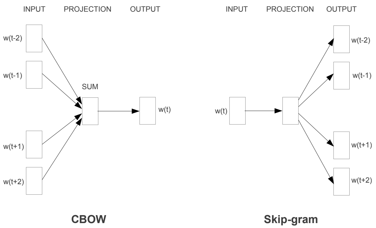
The following figure (source) shows shows a visualization of this architecture and the two modeling directions: CBOW and Skip-gram. In CBOW (left side of the figure), multiple context words such as \(w(t-2), w(t-1), w(t+1),\) and \(w(t+2)\) are aggregated to predict the central target word \(w(t)\). In Skip-gram (right side of the figure), the target/central word \(w(t)\) is fed in as input and the surrounding context words within a given window are predicted as output — both using the same embedding space to learn distributed representations of words.
Interpretability of the Embedding Space
-
Through iterative training across billions of word pairs, the model learns embeddings such that:
- Words that appear in similar contexts have similar directions in the vector space.
- Analogous relationships are captured through vector offsets.
- Syntactic categories (e.g., plurals, verb tenses) and semantic groupings (e.g., cities, countries) naturally emerge as clusters.
-
For instance, after training, the vectors for [“Paris”, “London”, “Berlin”] form a subspace distinct from [“France”, “UK”, “Germany”], yet maintain parallel structure, enabling analogical reasoning such as:
Word2Vec Architectures
-
Word2Vec offers two distinct neural architectures for learning word embeddings, as introduced by Mikolov et al. (2013) and further detailed in their follow-up paper, Distributed Representations of Words and Phrases and their Compositionality:
- Continuous Bag-of-Words (CBOW)
- Continuous Skip-gram (Skip-gram)
- Both are trained on the same corpus using similar mechanisms but differ in the direction of prediction — that is, whether the model predicts the center word from its context words or the context words from the center word. Both CBOW and Skip-gram learn embeddings that reflect word meaning through context prediction.
- CBOW excels in efficiency and stability for frequent words, while Skip-gram provides richer embeddings for rare words. Together, they form the foundation of Word2Vec’s success — enabling scalable and semantically powerful word representations.
Continuous Bag-of-Words (CBOW)
-
Concept:
- The CBOW model predicts the target (center) word based on the words surrounding it.
- Given a window of context words \(C_t = {w_{t-c}, \ldots, w_{t-1}, w_{t+1}, \ldots, w_{t+c}}\), the goal is to maximize:
- This makes CBOW a context-to-word model — the inverse of Skip-gram.
-
Architecture:
- The following figure (source) shows the CBOW model, where multiple context word one-hot vectors are fed into a shared embedding matrix, averaged, and used to predict the central target word.
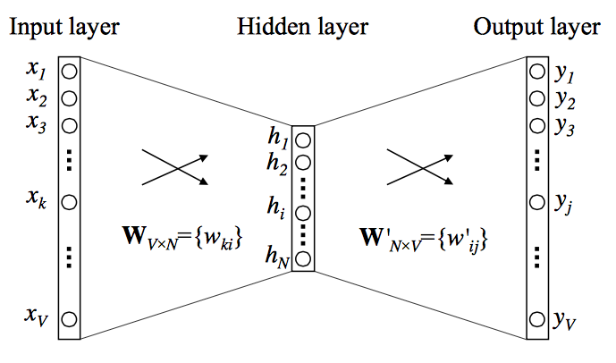
- Mathematically, the average of the context word vectors is computed as:
- The probability of predicting the target word \(w_t\) given this averaged context is then defined using the softmax function:
-
Learning Objective:
- The model’s training objective is to maximize the log-likelihood of all observed target words given their contexts over the entire corpus:
-
where:
- \(T\): total number of words (training instances) in the corpus.
- \(t\): index of the current target word position in the sequence.
- \(w_t\): the target (center) word being predicted.
- \(C_t\): the set of surrounding context words within the window size \(c\), i.e., \({w_{t-c}, \ldots, w_{t-1}, w_{t+1}, \ldots, w_{t+c}}\).
- \(p(w_t \mid C_t)\): the conditional probability of predicting the target word \(w_t\) given its context, computed via the softmax function.
- \(\log p(w_t \mid C_t)\): the log-likelihood term, used to penalize incorrect predictions smoothly.
- \(\mathcal{L}_{CBOW}\): the overall average log-likelihood objective that the model seeks to maximize during training.
-
Intuitively, this means CBOW learns embeddings that make the correct target word highly probable given its neighboring context — effectively maximizing the model’s ability to predict real word–context co-occurrences.
-
Gradients are propagated to update both input (\(v_w\)) and output (\(u_w\)) embeddings via stochastic gradient descent.
-
Parameterization:
-
For a given word index \(k\) in vocabulary \(V\), the referenced word is represented as:
- Input vector \(v_w = W_{(k, .)}\)
- Output vector \(u_w = W'_{(., k)}\)
-
The hidden layer has \(N\) neurons, and the model learns weight matrices \(W \in \mathbb{R}^{V \times N}\) and \(W' \in \mathbb{R}^{N \times V}\).
-
-
Overall Formula:
\[p(w_i | c) = y_i = \frac{e^{u_i}}{\sum_{i=1}^V e^{u_i}}, \quad \text{where } u_i = u_{w_i}^T v_c\]
Continuous Skip-gram (SG)
-
Concept:
- The Skip-gram model reverses CBOW’s direction: instead of predicting the target from the context, it predicts context words from the center word.
-
Architecture:
- The following figure (source) shows the structure of both Word2Vec architectures side-by-side: CBOW, which predicts the current word based on its context, and skip-gram, which predicts the surrounding words given the current word.
-
Softmax Prediction:
-
Recall that each word in Word2Vec has two representations: an input vector \(v_w\) for when it serves as the target (center) word, and an output vector \(u_w\) for when it appears as a context word.
-
Each target–context pair \((w_t, w_{t+j})\) is modeled as:
\[p(w_{t+j} | w_t) = \frac{\exp(u_{w_{t+j}}^T v_{w_t})} {\sum_{w' \in V} \exp(u_{w'}^T v_{w_t})}\]-
where:
- \(w_t\): the target (center) word.
- \(w_{t+j}\): a context word within a window of size \(c\) around \(w_t\).
- \(v_{w_t}\): the input embedding of the target word \(w_t\).
- \(u_{w_{t+j}}\): the output embedding of the context word \(w_{t+j}\).
- \(V\): the entire vocabulary.
- \(\exp(u_{w_{t+j}}^T v_{w_t})\): measures the similarity (via dot product) between the target and context embeddings in the exponentiated space.
- \(\sum_{w' \in V} \exp(u_{w'}^T v_{w_t})\): the normalization term ensuring the probabilities sum to 1 over all possible context words.
-
-
-
Learning Objective:
-
The Skip-gram objective is to maximize the log-likelihood of context words given the center word \(w_t\) over the entire corpus:
\[\mathcal{L}_{SG} = \frac{1}{T} \sum_{t=1}^{T} \sum_{-c \le j \le c, j \ne 0} \log p(w_{t+j} | w_t)\]- where:
- \(T\): total number of words (training samples) in the corpus.
- \(c\): context window size, determining how many words on each side of \(w_t\) are considered as context.
- \(w_t\): the center (target) word at position \(t\).
- \(w_{t+j}\): a context word at an offset \(j\) from the center word.
- \(p(w_{t+j} \mid w_t)\): the probability of observing the context word \(w_{t+j}\) given the center word \(w_t\), modeled using a softmax over the vocabulary.
- \(\log\): the natural logarithm, used to convert the product of probabilities into a sum for numerical stability and optimization.
- where:
-
Here, every occurrence of a word generates multiple (target \(\rightarrow\) context) prediction pairs, which makes training computationally heavier but more expressive — particularly for rare words.
-
Comparison: CBOW vs. Skip-gram
| Aspect | CBOW | Skip-gram |
|---|---|---|
| Prediction Direction | Context \(\rightarrow\) Target | Target \(\rightarrow\) Context |
| Input | Multiple context words | Single target word |
| Output | One target word | Multiple context words |
| Training Speed | Faster | Slower |
| Works Best For | Frequent words; large datasets/corpora | Rare words; small datasets/corpora |
| Robustness | Smoother embeddings | More detailed embeddings |
| Objective Function | \(\log p(w_t \mid C_t)\) | \(\sum_{-c \le j \le c, j \ne 0} \log p(w_{t+j} \mid w_t)\) |
Why Skip-gram Handles Rare Words and Small Datasets Better
-
Skip-gram updates the embeddings of the center (target) word for each of its context words, meaning that every occurrence of a word — even a rare one — produces multiple training examples. Each (target, context) pair contributes a separate gradient update, allowing the model to refine the embedding of infrequent words through repeated exposure to their surrounding context.
-
By contrast, CBOW treats rare words as targets to be predicted from their neighboring words. Because uncommon words appear less frequently as targets, they are updated fewer times and often with noisy or insufficient context, leading to less accurate representations.
-
In small datasets or corpora, this distinction becomes even more critical. With limited training data, rare words might occur only a few times. Skip-gram’s multiple updates per occurrence help compensate for data scarcity by amplifying each word’s learning signal. CBOW, however, struggles in such settings since it relies on aggregating context signals to predict sparse targets — an approach that benefits more from large, diverse corpora.
-
Example:
- In the sentence “The iguana basked on the rock,” the rare word iguana generates multiple Skip-gram training pairs — (iguana \(\rightarrow\) the), (iguana \(\rightarrow\) basked), (iguana \(\rightarrow\) on), (iguana \(\rightarrow\) rock) — each producing an update to its embedding.
- Under CBOW, iguana would be predicted only once from the context {the, basked, on, rock}, resulting in fewer gradient updates and weaker representation learning, especially in a small corpus.
Which Model to Use When
-
Use CBOW when:
- The dataset is large and contains many frequent words.
- You require fast training and smoother embeddings.
- The task emphasizes semantic similarity among common words (e.g., topic clustering, document similarity).
- Example: Training on Wikipedia or Common Crawl for general-purpose embeddings.
-
Use Skip-gram when:
- The dataset is smaller or contains many rare and domain-specific words.
- Skip-gram performs better in such cases because it creates multiple training pairs for each occurrence of a rare word, giving it more opportunities to learn meaningful relationships from limited data.
- You want to capture fine-grained syntactic or semantic nuances.
- The focus is on representation quality rather than speed.
- Example: Training embeddings for biomedical text, legal documents, or historical corpora.
-
Hybrid Strategy:
- Some implementations begin with CBOW pretraining and fine-tune with Skip-gram for precision.
- For multilingual or low-resource settings, Skip-gram tends to outperform due to its capacity to learn richer embeddings from detailed contextual cues using fewer examples.
Training and Optimization
-
The training of Word2Vec centers on optimizing word embeddings so that they accurately predict contextual relationships between words. Each word in the vocabulary is assigned two learnable vectors: one for when it acts as a target (input) word and another for when it acts as a context (output) word. These vectors are iteratively updated during training to maximize the probability of observed word–context pairs (equivalently, to maximize the log-likelihood of correct predictions). In implementation, this is often expressed as minimizing the negative log-likelihood loss, which is the inverse of the same objective.
-
However, training Word2Vec models efficiently is challenging, especially with large vocabulary sizes. Mikolov et al. (2013) introduced key approximation strategies — most notably negative sampling and hierarchical softmax — that make large-scale training computationally feasible while maintaining embedding quality. These techniques drastically reduce the cost of computing softmax over all vocabulary words by focusing updates on a small subset of informative examples.
Objective Function
-
The central goal of Word2Vec is to maximize the likelihood of predicting correct word–context pairs.
- In the Skip-gram model, the network predicts surrounding context words given a target word.
- In the CBOW model, it predicts the target word given its surrounding context.
-
Each word \(w\) in the vocabulary is represented by two embeddings:
- \(v_w\): the input vector, used when the word serves as the target (center) word.
- \(u_w\): the output vector, used when the word serves as a context word to be predicted.
-
The Skip-gram objective maximizes the average log-probability of observing context words around each target word:
\[\mathcal{L}_{SG} = \frac{1}{T} \sum_{t=1}^{T} \sum_{-c \le j \le c, j \ne 0} \log p(w_{t+j} | w_t)\] -
The CBOW objective instead maximizes the log-probability of the target word given its surrounding context:
\[\mathcal{L}_{CBOW} = \frac{1}{T} \sum_{t=1}^{T} \log p(w_t | C_t)\] -
In both models, the conditional probability is computed using the softmax function:
\[p(w_o | w_i) = \frac{\exp(u_{w_o}^T v_{w_i})} {\sum_{w' \in V} \exp(u_{w'}^T v_{w_i})}\]-
where:
- \(v_{w_i}\): input (target) word vector.
- \(u_{w_o}\): output (context) word vector.
- \(T\): total number of words in the training corpus.
- \(c\): context window size, defining how many words to the left and right are considered.
- \(w_t\): the target (center) word at position \(t\).
- \(w_{t+j}\): a context word located \(j\) positions away from the target.
- \(C_t\): the set of context words surrounding \(w_t\).
- \(V\): the vocabulary containing all unique words.
- \(p(w_o \mid w_i)\): the model’s predicted probability of observing context word \(w_o\) given target word \(w_i\).
-
-
The model thus maximizes the log-likelihood that true word–context pairs occur more frequently than random combinations, effectively shaping the embedding space to reflect semantic relationships.
Why the Full Softmax Is Computationally Expensive
- The denominator of the naive softmax function used in CBOW and Skip-gram requires computing the normalization term over all words in the vocabulary (\(V\)): \(\sum_{w' \in V} \exp(u_{w'}^T v_{w_I})\).
- For a large vocabulary (where \(\mid V \mid\) can exceed millions, say \(10^5\) to \(10^7\)), this becomes computationally intractable because the denominator must be recalculated for every training pair.
- To address this, Mikolov et al. (2013) introduced two key approximation methods: Hierarchical Softmax and Negative Sampling.
Hierarchical Softmax
- Hierarchical Softmax, introduced by Morin and Bengio (2005) and later applied by Mikolov et al. (2013), is an efficient alternative to the standard softmax layer used in language models.
Concept
-
Hierarchical Softmax replaces the flat softmax layer with a binary tree structure—typically a Huffman tree built using word frequencies. Each word is represented as a leaf node, and the model computes the probability of a word by traversing the path from the root to the corresponding leaf.
-
The probability of selecting a word is modeled as the product of probabilities of binary decisions made at each internal node along this path. This significantly reduces computational cost, especially in settings with very large vocabularies.
Loss Function
- Recall that each word in Word2Vec has two representations: an input vector \(v_w\) for when it serves as the target (center) word, and an output vector \(u_w\) for when it appears as a context word.
- For a given target word \(w\) and its input vector \(v_{w_t}\), let the path from the root of the Huffman tree to \(w\) pass through internal nodes \(n_1, n_2, \dots, n_L\).
- At each internal node \(n_i\), a binary decision \(d_i \in {0,1}\) determines whether to move left (0) or right (1). The conditional probability of word \(w\) given the target \(w_t\) is:
-
Alternatively, using node-indexed notation:
\[p(w \mid w_i) = \prod_{j=1}^{L(w)-1} \sigma \left( \text{dir}(n(w,j+1)) \cdot u_{n(w,j)}^T v_{w_i} \right)\] -
where:
- \(v_{w_t}\): input vector of the target word.
- \(u_{n_i}\): output vector of internal node \(n_i\).
- \(L(w)\): path length from the root to word \(w\).
- \(d_i\): binary decision at node \(n_i\) (0 = left, 1 = right).
- \(n(w,j)\): \(j^{th}\) node along the path to \(w\).
- \(\sigma(x) = \frac{1}{1 + e^{-x}}\): sigmoid function mapping scores to probabilities.
- This loss function expresses the probability of reaching a leaf node (the target word) in the hierarchical softmax tree by multiplying the sigmoid probabilities of each binary decision along the path. The training objective maximizes this probability — equivalently, the log-likelihood of the correct word given its context.
Advantages
- Reduces computational complexity from \(O(\mid V \mid)\) to \(O(\log \mid V \mid)\).
- Frequent words (shorter paths) are processed faster during training.
Disadvantages
- More complex implementation compared to flat softmax.
- Rare words (longer paths) involve more computations.
Negative Sampling
- Negative Sampling, introduced by Mikolov et al. (2013) in their second Word2Vec paper, is an efficient alternative to softmax for training word embeddings. It reframes the prediction task as a binary classification problem, allowing the model to focus on distinguishing real word-context pairs from artificially generated ones.
Concept
-
Instead of computing probabilities across the entire vocabulary (as in softmax), Negative Sampling reframes training as a binary classification task: the model learns to distinguish genuine word-context pairs (positive samples) from randomly generated pairs (negative samples).
-
For each true pair of words \((w_i, w_o)\): where \(w_i\) is the input (target) word and \(w_o\) is the output (context) word — the model samples \(K\) negative words \(w_1', w_2', \ldots, w_K'\) from a noise distribution (commonly proportional to word frequency raised to the power of \(\tfrac{3}{4}\)).
-
During each training step, the model updates only a small subset of embeddings:
- The input vector \(v_{w_i}\) of the current target word, since it is directly involved in all dot products for that step.
- The output vector \(u_{w_o}\) of the positive (true) context word, which is reinforced to align more closely with \(v_{w_i}\).
- The output vectors \(u_{w_1'}, \ldots, u_{w_K'}\) of the sampled negative words, which are adjusted in the opposite direction to reduce similarity with \(v_{w_i}\).
-
All other words in the vocabulary remain untouched during that iteration. This sparse parameter update is what makes negative sampling dramatically more efficient than the full softmax computation, which would otherwise require updating every output vector in the vocabulary.
Loss Function
- The loss function for one positive pair \((w_i, w_o)\) and \(K\) negative samples \((w_1', \ldots, w_K')\) is defined as:
-
Alternatively, in expectation form over the noise distribution:
\[\mathcal{L}_{NS} = -\left[ \log \sigma(u_{w_o}^T v_{w_i}) + \sum_{k=1}^{K} \mathbb{E}_{w_k' \sim P_n(w)} \log \sigma(-u_{w_k'}^T v_{w_i}) \right]\]-
where:
- \(v_w\): input vector of word \(w\) (used when it is the target word).
- \(u_w\): output vector of word \(w\) (used when it is a context word).
- \(\sigma(x) = \frac{1}{1 + e^{-x}}\): sigmoid function mapping similarity scores to probabilities.
- \(u_{w_o}^T v_{w_i}\): dot product measuring similarity between target and context embeddings.
- \(w_i\): target (center) word currently being processed.
- \(w_o\): true context word co-occurring with \(w_i\) (positive sample).
- \(w_k'\): negative words sampled from the noise distribution.
- \(K\): number of negative samples per positive pair.
- \(P_n(w) = \frac{f(w)^{3/4}}{Z}\): noise distribution used for sampling negatives, with \(f(w)\) as word frequency and \(Z\) a normalization constant.
- \(\mathcal{L}_{NS}\): negative sampling loss, minimized during training to make positive pairs more similar and negative pairs more dissimilar.
-
-
This formulation ensures that positive word-context pairs yield large dot products (so \(\sigma(u_{w_o}^T v_{w_i}) \approx 1\)), while negative pairs yield small dot products (so \(\sigma(-u_{w_k}^T v_{w_i}) \approx 1\)).
Intuition
- Positive pairs are optimized to have higher dot products, pulling their embeddings closer in vector space.
- Negative pairs are optimized to have lower dot products, pushing their embeddings apart.
- This leads to embeddings where semantically similar words are close together, while dissimilar ones are far apart.
Advantages
- Extremely efficient—updates are limited to a small subset of the vocabulary.
- Requires only 5–20 negative samples per step to perform well.
- Empirically matches or exceeds the performance of Hierarchical Softmax in many NLP tasks.
- Highly parallelizable, making it well-suited for GPU acceleration.
Disadvantages
- Does not model a full probability distribution over the vocabulary.
- Primarily useful for embedding learning, not for tasks requiring normalized probabilities.
Subsampling of Frequent Words
- High-frequency words such as “the,” “of,” and “and” appear so often that they dominate the training process without adding semantic value.
-
To address this, Mikolov et al. proposed randomly discarding frequent words with probability:
\[P(w_i) = 1 - \sqrt{\frac{t}{f(w_i)}}\]- where \(t\) is a threshold typically \(10^{-5}\), and \(f(w_i)\) is the relative frequency of word \(w_i\).
- This reduces training time and improves vector quality for less frequent words.
Related: Parallelization and Efficiency
- While not an “optimization” technique per se, Word2Vec’s architecture is ideal for parallelization.
- Each word–context pair can be processed independently.
- Distributed implementations (such as in Gensim and TensorFlow) leverage multi-core and GPU computation.
- Training large models (e.g., Google News corpus with 100 billion words) typically converges within hours on standard hardware.
Comparative Analysis: Optimization Techniques
| Technique | Goal | Complexity | Typical Use Case |
|---|---|---|---|
| Hierarchical Softmax | Efficient probability computation | \(\mathcal{O}(\log V)\) | When accurate probabilities are needed |
| Negative Sampling | Efficient gradient updates | \(\mathcal{O}(k)\) | When only vector similarity is needed |
| Subsampling | Reduce bias from common words | \(\mathcal{O}(1)\) | Large corpora with many stopwords |
Embedding and Semantic Relationships
-
Word2Vec’s training process produces a set of word vectors (embeddings) that encode semantic and syntactic information in a continuous, semantically meaningful geometric space.
- Proximity represents similarity of meaning.
- Direction represents relational structure.
- Linear operations capture analogies and transformations.
- This property makes Word2Vec a cornerstone in modern NLP — providing not only compact word representations but also interpretable relationships that reflect the way humans understand language.
- These embeddings are powerful because they convert discrete linguistic units (words) into numerical representations that reflect meaning, contextual similarity, and linguistic regularities.
From Co-occurrence to Geometry
-
During training, Word2Vec positions each word vector \(v_w \in \mathbb{R}^N\) such that words occurring in similar contexts are close to each other in the embedding space.
-
Mathematically, if two words \(w_i\) and \(w_j\) share similar context distributions, their conditional probabilities \(p(C \mid w_i)\) and \(p(C \mid w_j)\) are alike, leading to embeddings with high cosine similarity:
- This means that words like dog and cat, which appear in similar linguistic environments (e.g., near words like pet, animal, food), will have vectors oriented in similar directions.
Linear Relationships and Analogy
- One of the most celebrated properties of Word2Vec embeddings is their ability to capture analogical relationships using simple linear algebra.
-
These relationships emerge naturally from the model’s predictive training objective, which enforces consistent geometric offsets between semantically related words.
- For instance:
- This implies that the relationship between “man” and “woman” is encoded as a directional vector offset in the space, and the same offset applies to other analogous pairs like:
Clustering and Semantic Neighborhoods
-
When visualized (e.g., using t-SNE or PCA), Word2Vec embeddings form clusters that group together semantically or syntactically similar words.
- Semantic clusters: Words such as dog, cat, horse, cow cluster under the broader concept of animals.
- Syntactic clusters: Words like running, swimming, jumping cluster based on grammatical function (verbs in gerund form).
-
In this space, semantic similarity corresponds to spatial proximity, and semantic relations correspond to vector directions.
Interpreting the Embedding Space
- The embedding space captures multiple types of relationships:
| Relationship Type | Example | Geometric Interpretation |
|---|---|---|
| Synonymy | happy ↔ joyful | Small cosine distance |
| Antonymy | good ↔ bad | Large angle, opposite directions |
| Hierarchical | car ↔ vehicle | “Parent–child” proximity |
| Analogical | king – man + woman ≈ queen | Consistent vector offset |
- This geometric consistency arises because the dot product \(u_{w_o}^T v_{w_i}\): central to Word2Vec’s loss function — forces the space to preserve relational proportionality among co-occurring words. For more theoretical grounding on this, see Levy and Goldberg (2014).
Example: Semantic Continuity
-
To illustrate, consider these relationships in trained embeddings:
\[v_{\text{France}} - v_{\text{Paris}} \approx v_{\text{Italy}} - v_{\text{Rome}}\] \[v_{\text{walking}} - v_{\text{walk}} \approx v_{\text{running}} - v_{\text{run}}\] -
Both examples demonstrate that semantic and syntactic transformations (capital–country or verb–tense) are encoded as parallel vectors in the embedding space.
Distinction from Traditional Models
- Word2Vec represents a fundamental paradigm shift from earlier count-based and probabilistic language models.
-
Traditional methods typically relied on explicit frequency counts or co-occurrence matrices, while Word2Vec learns distributed representations that are continuous, dense, and semantically meaningful. Word2Vec diverges from traditional models by:
- Moving from counting to predicting, thus learning generalized patterns.
- Embedding words in a continuous space, allowing geometric interpretation.
- Capturing semantics and syntax simultaneously, through context-based optimization.
- These distinctions made Word2Vec the first widely adopted neural representation model, bridging the gap between symbolic and distributed semantics in NLP.
Traditional Count-based Models
-
Before neural embeddings, most language representations were derived from word frequency statistics.
-
Co-occurrence Matrices:
-
These models record how often each word appears with every other word in a fixed context window.
-
The resulting matrix \(M \in \mathbb{R}^{\mid V \mid \times \mid V \mid}\) has entries:
\[M_{ij} = \text{count}(w_i, w_j)\]- where \(\text{count}(w_i, w_j)\) denotes how many times word \(w_j\) occurs near word \(w_i\).
-
High-dimensional and extremely sparse, these matrices often undergo dimensionality reduction (e.g., SVD or PCA) to extract latent features.
-
-
TF-IDF Representations (Salton (1988)):
-
Assign weights to words based on their document-specific frequency and global rarity:
\[\text{TF-IDF}(t, d) = \text{TF}(t, d) \times \log\frac{N}{\text{DF}(t)}\] -
Useful for document retrieval, but insensitive to word order or semantic relationships.
-
-
Topic Models (e.g., LDA) (Blei et al. (2003)):
- Represent documents as mixtures of latent “topics” inferred through probabilistic modeling.
- While they uncover thematic structure, they don’t provide fine-grained word-level semantics or geometric relationships.
-
Predictive vs. Count-based Philosophy
-
The essential distinction is predictive learning versus statistical counting:
Feature Count-based Models (e.g., TF-IDF, LSA) Predictive Models (Word2Vec) Representation Sparse, frequency-based Dense, distributed Learning Objective Approximate co-occurrence statistics Predict neighboring words Captures Context Implicitly via counts Explicitly via prediction Semantic Structure Limited, global Rich, local and continuous Computational Method Matrix decomposition Neural optimization Output Dimensionality Fixed by vocabulary Tunable (e.g., 100–300 dimensions) -
Key insight: Count-based models memorize co-occurrence patterns, while Word2Vec learns to predict them. This predictive training enables the embeddings to generalize beyond exact word occurrences — capturing unseen but semantically related patterns.
Connection to Matrix Factorization
- Although Word2Vec is trained as a neural prediction model, it is mathematically related to implicit matrix factorization.
-
As shown by Levy and Goldberg (2014), the Skip-gram with Negative Sampling (SGNS) objective implicitly factorizes a shifted Pointwise Mutual Information (PMI) matrix between words and their contexts.
- The PMI between a word \(w\) and a context \(c\) is defined as:
- Recall that each word in Word2Vec has two representations: an input vector \(v_w\) for when it serves as the target (center) word, and an output vector \(u_w\) for when it appears as a context word.
-
During training, the model optimizes these such that:
\[v_w^T u_c \approx \text{PMI}(w, c) - \log k\]-
where:
- \(v_w\): embedding of the word when it appears as the center (target)
- \(u_c\): embedding of the word when it appears as a context word
- \(v_w^T u_c\): dot product representing the similarity or association strength between \(w\) and \(c\)
- \(\text{PMI}(w, c)\): Pointwise Mutual Information, measuring how much more often \(w\) and \(c\) co-occur than expected by chance
- \(P(w, c)\): empirical joint probability of seeing \(w\) and \(c\) together
- \(P(w)\), \(P(c)\): marginal probabilities of the individual word and context
- \(k\): number of negative samples used in SGNS training
- \(\log k\): the shifting term that adjusts the PMI to account for negative sampling
-
- Thus, Word2Vec implicitly factorizes a smoothed and shifted PMI matrix, yielding low-dimensional embeddings that capture co-occurrence statistics—without ever constructing the matrix explicitly.
Contextual Encoding and Generalization
-
Traditional models treat each word as an independent symbol; the model cannot infer that doctor and physician are semantically related. In contrast, Word2Vec represents both words as nearby vectors because they occur in similar contexts, such as hospital, patient, or medicine.
-
This contextual generalization enables tasks like:
- Synonym detection (high cosine similarity)
- Analogy reasoning (vector offsets)
- Clustering and semantic grouping
-
These capabilities were not achievable with bag-of-words or count-based models, which lacked a mechanism to encode relational meaning.
Computational Perspective
-
Word2Vec also introduced major computational improvements:
- Scalability: The use of negative sampling and hierarchical softmax allows training on billions of words efficiently.
- Memory Efficiency: Each word is represented by compact \(N\)-dimensional vectors (e.g., 300 dimensions) instead of huge sparse vectors.
- Incremental Learning: Embeddings can be updated online, unlike matrix factorization, which must process entire corpora at once.
Semantic Nature of Word2Vec Embeddings
-
Word2Vec embeddings are semantic in nature because they encode meaningful relationships between words based on their distributional context. Rooted in the distributional hypothesis — the idea that “words appearing in similar contexts tend to have similar meanings” (Harris (1954))—Word2Vec learns to embed words in a vector space by predicting their surrounding context. This training objective forces words with similar usage to acquire similar vector representations.
-
This training objective forces words with similar usage to acquire similar vector representations.
-
As a result, the geometry of the embedding space captures semantic similarity through distance, and analogical relationships through direction. These geometric properties enable a wide range of linguistic tasks, such as clustering similar words, solving analogies, and performing semantic reasoning, all via simple vector operations.
-
Together, these capabilities make Word2Vec one of the earliest and most intuitive examples of how neural networks can internalize and represent linguistic meaning through learned representations.
How Semantic Meaning Emerges
- During training, each word \(w_t\) is optimized such that its embedding \(v_{w_t}\) maximizes the likelihood of co-occurring context words \({w_{t+j}}\).
-
As a result, words that occur in similar environments receive similar gradient updates, causing their vectors to align in space.
- Formally, if two words \(w_a\) and \(w_b\) share overlapping context distributions:
- … then their embeddings converge to similar directions:
- This geometric proximity encodes semantic relatedness — the closer the vectors, the more semantically similar the words.
CBOW and Skip-gram as Semantic Learners
-
CBOW Model:
- Predicts a target word given its context.
- Learns smoother embeddings by averaging contextual information, leading to stable semantic representations for frequent words.
- Example: Predicting “mat” from the context “The cat sat on the ___” helps reinforce relationships between cat, sat, and mat.
-
Skip-gram Model:
- Predicts multiple context words from a single target.
- Captures more fine-grained semantic details, especially for rare words.
- Example: Given “cat”, Skip-gram learns to predict “the”, “sat”, “on”, and “mat”, enriching cat’s embedding through diverse contextual associations.
- Together, these architectures operationalize the distributional hypothesis through context-based prediction, transforming textual co-occurrence patterns into structured vector relationships.
Types of Semantic Relationships Captured
- Similarity:
- Words with related meanings are embedded close together. For * instance, dog, cat, and puppy form a tight cluster in the embedding space due to shared usage contexts.
- Analogy:
- Linear relationships in vector space reflect semantic analogies such as:
- This pattern generalizes across many relationships (capital–country, gender, verb tense, etc.), e.g.:
- Clustering:
-
Semantic similarity also manifests as clusters within the high-dimensional space:
- Animals: {dog, cat, horse, cow}
- Countries: {France, Germany, Italy, Spain}
- Emotions: {happy, joyful, cheerful, glad}
-
Clustering results from the model’s ability to map semantically related words to nearby regions in the embedding space.
-
Geometric and Semantic Interpretations
- Each semantic relationship has a geometric counterpart:
| Relationship Type | Example | Geometric Interpretation |
|---|---|---|
| Synonymy | car ↔ automobile | Small cosine distance |
| Analogy | man \(\rightarrow\) woman :: king \(\rightarrow\) queen | Parallel vector offset |
| Hypernymy | dog \(\rightarrow\) animal | Direction along hierarchical axis |
| Antonymy | good ↔ bad | Large angular separation |
| Morphology | walk \(\rightarrow\) walking | Consistent offset along tense dimension |
- This shows that semantics are encoded directionally and proportionally in the embedding space — a key reason Word2Vec embeddings are interpretable through vector arithmetic.
Analogy through Vector Arithmetic
- Word2Vec’s training objective aligns embedding directions in such a way that analogical reasoning emerges naturally.
- If a relationship between two words is represented as a consistent vector offset, then:
- For example:
- This reveals a kind of semantic isomorphism — a structural preservation of relationships across conceptual domains.
Limitations and Advances
-
Word2Vec remains one of the most influential frameworks in the evolution of NLP, revolutionizing the field with its ability to encode meaning geometrically. By representing words as continuous vectors in a semantic space, it enabled machines to understand words not merely as symbolic tokens, but as entities with inherent relationships and structure.
-
However, despite its groundbreaking impact, Word2Vec’s design introduces several inherent limitations that eventually spurred the development of more advanced contextualized embedding models. These limitations stem primarily from its static and context-independent nature—each word is assigned a single vector, regardless of its varying meanings in different contexts. Additionally, Word2Vec’s approach to processing context and dealing with data sparsity posed further challenges in capturing nuanced language use.
-
To address these shortcomings, newer models emerged that not only capture the general meaning of words but also adapt dynamically to their context within a sentence or document. These contextualized embeddings now form the foundation of modern NLP, offering a far more flexible and precise understanding of language.
Static, Non-Contextualized Nature
-
Single Vector per Word:
- In Word2Vec, each word type is represented by one fixed embedding, regardless of the sentence or context in which it appears.
- For instance, the word “bank” is assigned a single vector whether it refers to a financial institution or the side of a river.
-
As a result, multiple senses of a word (polysemy) are collapsed into a single point in the embedding space.
- Mathematically, for all occurrences of a word \(w\), Word2Vec assigns one embedding \(v_w \in \mathbb{R}^N\), such that \(v_w = f(w)\), independent of its local context.
- This static representation means that semantic disambiguation is impossible within the model itself.
-
Combination of Contexts:
- Because all usages of a word are averaged during training, the resulting embedding represents an aggregate of multiple meanings.
- For example, “apple” in “Apple released a new iPhone” (corporate sense) and “I ate an apple” (fruit sense) are both used to update the same embedding vector.
- The consequence is a semantic compromise — embeddings become blurry averages of distinct meanings.
-
Lack of Contextual Adaptation:
- Word2Vec’s fixed-size context window only captures local co-occurrence statistics, not long-range dependencies or sentence-level structure.
-
Thus, the model cannot adapt a word’s meaning dynamically based on its syntactic role or broader discourse context.
- Example:
- “She read a book.”
- “He will book a flight.” Word2Vec assigns nearly identical vectors to “book” in both cases, even though one is a noun and the other a verb.
Training Process and Computational Considerations
-
Training Adjustments:
- Throughout training, Word2Vec adjusts embeddings through stochastic gradient descent to improve co-occurrence prediction accuracy.
- However, these updates are purely statistical — not semantic — meaning the model refines embeddings globally rather than creating distinct sense representations.
-
Computational Demands:
- Although optimized via negative sampling, training large vocabularies (millions of words) still requires significant computational resources and memory.
- Furthermore, retraining or updating embeddings for new corpora often demands complete reinitialization, since Word2Vec lacks an efficient fine-tuning mechanism.
Handling of Special Cases
-
Phrase and Idiom Representation:
- Word2Vec struggles with multi-word expressions or idioms whose meanings are non-compositional.
- For instance, “hot potato” or “New York Times” cannot be represented by simply averaging the vectors of their component words.
- As proposed by Mikolov et al. (2013), one partial solution was to treat frequent phrases as single tokens using statistical co-occurrence detection.
-
Out-of-Vocabulary (OOV) Words:
- Word2Vec cannot generate embeddings for words not seen during training.
- This limitation is particularly problematic for morphologically rich or non-segmented languages.
- Later models such as FastText addressed this by representing words as compositions of character n-grams, allowing generalization to unseen forms.
Global Vector Representation Limitations
-
Uniform Representation Across Contexts:
- Word2Vec, like GloVe, produces a global vector for each word.
- This uniformity neglects that a word’s meaning shifts with context.
- For example, the embeddings for “light” cannot distinguish between “light weight” and “light bulb.”
-
Sentiment Polarity and Context Sensitivity:
- Because Word2Vec relies on unsupervised co-occurrence statistics, it can place antonyms such as “good” and “bad” near each other if they occur in similar syntactic positions.
- This leads to issues in sentiment analysis tasks, where distinguishing polarity is essential.
- Tang et al. (2014) proposed Sentiment-Specific Word Embeddings (SSWE), which integrate polarity supervision into the loss function to separate words by sentiment.
Resulting Embedding Compromises
- The outcome of these constraints is that Word2Vec embeddings, though semantically meaningful on average, are context-agnostic and therefore less precise for downstream tasks requiring nuanced interpretation. This trade-off — efficiency and generality versus contextual precision — defined the next phase of NLP research.
Advances Beyond Word2Vec
-
To overcome these challenges, newer models introduced contextualized embeddings, where a word’s representation dynamically changes depending on its sentence-level context.
-
GloVe (Global Vectors for Word Representation):
- Combines local co-occurrence prediction (like Word2Vec) with global matrix factorization.
- Encodes both semantic relationships and global corpus statistics.
- A detailed discourse of this embedding technique has been offered in the Global Vectors for Word Representation (GloVe) section.
-
FastText:
- Represents words as the sum of subword (character n-gram) embeddings, enabling generalization to unseen or rare words.
- Particularly effective for morphologically rich languages.
- A detailed discourse of this embedding technique has been offered in the FastText section.
-
ELMo (Embeddings from Language Models):
- Generates context-dependent embeddings using a bidirectional LSTM language model.
- A word’s vector \(v_{w, \text{context}}\) depends on its surrounding sentence, allowing dynamic sense representation.
-
BERT (Bidirectional Encoder Representations from Transformers):
- Leverages the Transformer architecture to model bidirectional context simultaneously.
- Each occurrence of a word is encoded uniquely as a function of the entire sequence, capturing fine-grained semantics, syntax, and disambiguation.
-
Formally, embeddings are contextualized as:
\[v_{w_i} = f(w_i, w_{1:T})\]- where \(f\) is a deep transformer function conditioned on the entire input sentence.
- A detailed discourse of this embedding technique has been offered in our BERT primer.
-
Computational Challenges and Approximations
- Although contextual models supersede Word2Vec conceptually, its innovations in efficient optimization remain foundational.
-
Word2Vec introduced practical strategies that allowed large-scale training long before transformer-based systems existed.
- Softmax Approximation Challenge
- Computing the denominator in the softmax function:
- required summing over the entire vocabulary, which is computationally infeasible for large corpora.
- Negative Sampling Solution
- Word2Vec replaced the full softmax with negative sampling, reframing prediction as a binary classification task:
- Here, positive word pairs are pulled closer in vector space, and random negative pairs are pushed apart — allowing efficient updates with only a few sampled words per step.
- Hierarchical Softmax
- An alternate efficiency method that organizes the vocabulary as a Huffman tree, reducing computational complexity from \(O(\mid V \mid)\) to \(O(\log \mid V \mid)\).
- Softmax Approximation Challenge
- These innovations enabled Word2Vec to scale to billions of tokens — laying the groundwork for subsequent neural representation learning.
Evolutionary Summary
| Generation | Example Models | Key Advancement |
|---|---|---|
| Count-based | TF-IDF, LSA | Frequency and co-occurrence statistics |
| Predictive Static | Word2Vec, GloVe, FastText | Distributed representations of word meaning |
| Contextualized | ELMo, BERT, GPT | Dynamic embeddings conditioned on full sentence context |
Additional Resources
- For a deeper exploration of Word2Vec, the following resources provide comprehensive insights into the foundational aspects of the algorithm:
Global Vectors for Word Representation (GloVe)
Overview
- Proposed in GloVe: Global Vectors for Word Representation by Pennington et al. (2014), Global Vectors for Word Representation (GloVe) embeddings are a type of word representation used in NLP. They are designed to capture not just the local context of words but also their global co-occurrence statistics in a corpus, thus providing a rich and nuanced word representation.
- By blending these approaches, GloVe captures a fuller picture of word meaning and usage, making it a valuable tool for various NLP tasks, such as sentiment analysis, machine translation, and information retrieval.
- Here’s a detailed explanation along with an example:
How GloVe Works
-
Co-Occurrence Matrix: GloVe starts by constructing a large matrix that represents the co-occurrence statistics of words in a given corpus. This matrix has dimensions of
[vocabulary size] x [vocabulary size], where each entry \((i, j)\) in the matrix represents how often word i occurs in the context of word j. -
Matrix Factorization: The algorithm then applies matrix factorization techniques to this co-occurrence matrix. The goal is to reduce the dimensions of each word into a lower-dimensional space (the embedding space), while preserving the co-occurrence information.
-
Word Vectors: The end result is that each word in the corpus is represented by a vector in this embedding space. Words with similar meanings or that often appear in similar contexts will have similar vectors.
-
Relationships and Analogies: These vectors capture complex patterns and relationships between words. For example, they can capture analogies like “man is to king as woman is to queen” by showing that the vector ‘king’ - ‘man’ + ‘woman’ is close to ‘queen’.
Example
- Imagine a simple corpus with the following sentences:
- “The cat sat on the mat.”
- “The dog sat on the log.”
- From this corpus, a co-occurrence matrix is constructed. For instance, ‘cat’ and ‘mat’ will have a higher co-occurrence score because they appear close to each other in the sentences. Similarly, ‘dog’ and ‘log’ will be close in the embedding space.
- After applying GloVe, each word (like ‘cat’, ‘dog’, ‘mat’, ‘log’) will be represented as a vector. The vector representation captures the essence of each word, not just based on the context within its immediate sentence, but also based on how these words co-occur in the entire corpus.
- In a large and diverse corpus, GloVe can capture complex relationships. For example, it might learn that ‘cat’ and ‘dog’ are both pets, and this will be reflected in how their vectors are positioned relative to each other and to other words like ‘pet’, ‘animal’, etc.
Significance of GloVe
- GloVe is powerful because it combines the benefits of two major approaches in word representation:
- Local Context Window Methods (like Word2Vec): These methods look at the local context, but might miss the broader context of word usage across the entire corpus.
- Global Matrix Factorization Methods: These methods, like Latent Semantic Analysis (LSA), consider global word co-occurrence but might miss the nuances of local word usage.
Limitations of GloVe
- While GloVe has been widely used and offers several rich word representations, it may not be the optimal choice for every NLP application, especially those requiring context sensitivity, handling of rare words, or efficient handling of computational resources as detailed below.
Lack of Context-Sensitivity
- Issue: GloVe generates a single, static vector for each word, regardless of the specific context in which the word is used. This can be a significant limitation, especially for words with multiple meanings (polysemy).
- Example: The word “bank” will have the same vector representation whether it refers to the side of a river or a financial institution, potentially leading to confusion in downstream tasks where context matters.
- Comparison: Modern models like BERT and GPT address this limitation by creating context-sensitive embeddings, where the meaning of a word can change based on the sentence or context in which it appears.
Inefficient for Rare Words
- Issue: GloVe relies on word co-occurrence statistics from large corpora, which means it may not generate meaningful vectors for rare words or words that don’t appear frequently enough in the training data.
- Example: Words that occur infrequently in a corpus will have less reliable vector representations, potentially leading to poor performance on tasks that involve rare or domain-specific vocabulary.
- Comparison: Subword-based models like FastText handle this limitation more effectively by creating word representations based on character n-grams, allowing even rare words to have meaningful embeddings.
Corpus Dependence
- Issue: The quality of the GloVe embeddings is highly dependent on the quality and size of the training corpus. If the corpus lacks diversity or is biased, the resulting word vectors will reflect these limitations.
- Example: A GloVe model trained on a narrow or biased dataset may fail to capture the full range of meanings or relationships between words, especially in domains or languages not well-represented in the corpus.
- Comparison: This issue is less pronounced in models like transformer-based architectures, where transfer learning allows fine-tuning on specific tasks or domains, reducing the dependence on a single corpus.
Computational Cost
- Issue: Training GloVe embeddings on large corpora involves computing and factorizing large co-occurrence matrices, which can be computationally expensive and memory-intensive.
- Example: The memory requirement for storing the full co-occurrence matrix grows quadratically with the size of the vocabulary, which can be prohibitive for very large datasets.
- Comparison: While Word2Vec also has computational challenges, GloVe’s matrix factorization step tends to be more resource-intensive than the shallow neural networks used by Word2Vec.
Limited to Word-Level Representation
- Issue: GloVe embeddings operate at the word level and do not directly handle subword information such as prefixes, suffixes, or character-level nuances.
- Example: Morphologically rich languages, where words can take many forms based on tense, gender, or plurality, may not be well-represented in GloVe embeddings.
- Comparison: FastText, in contrast, incorporates subword information into its word vectors, allowing it to better represent words in languages with complex morphology or in cases where a word is rare but its root form is common.
Inability to Handle OOV (Out-of-Vocabulary) Words
- Issue: Since GloVe produces fixed embeddings for words during the training phase, it cannot generate embeddings for words that were not present in the training corpus, known as Out-of-Vocabulary (OOV) words.
- Example: If a new or domain-specific word is encountered during testing or inference, GloVe cannot generate a meaningful vector for it.
- Comparison: Subword-based models like FastText or context-based models like BERT can mitigate this problem by creating embeddings dynamically, even for unseen words.
fastText
Overview
- Proposed in Enriching Word Vectors with Subword Information by Bojanowski et al. (2017), fastText is an advanced word representation and sentence classification library developed by Facebook AI Research (FAIR). It’s primarily used for text classification and word embeddings in NLP. fastText differs from traditional word embedding techniques through its unique approach to representing words, which is particularly beneficial for understanding morphologically complex languages or handling rare words.
- Specifically, fastText’s innovative approach of using subword information makes it a powerful tool for a variety of NLP tasks, especially in dealing with languages that have extensive word forms and in situations where the dataset contains many rare words. By learning embeddings that incorporate subword information, fastText provides a more nuanced and comprehensive understanding of language semantics compared to traditional word embedding methods.
- Here’s a detailed look at fastText with an example.
Core Features of fastText
-
Subword Information: Unlike traditional models that treat words as the smallest unit for training, fastText breaks down words into smaller units - subwords or character n-grams. For instance, for the word “fast”, with a chosen n-gram range of 3 to 6, some of the subwords would be “fas”, “fast”, “ast”, etc. This technique helps in capturing the morphology of words.
-
Handling of Rare Words: Due to its subword approach, fastText can effectively handle rare words or even words not seen during training. It generates embeddings for these words based on their subword units, allowing it to infer some meaning from these subcomponents.
-
Efficiency in Learning Word Representations: fastText is efficient in learning representations for words that appear infrequently in the corpus, which is a significant limitation in many other word embedding techniques.
-
Applicability to Various Languages: Its subword feature makes it particularly suitable for languages with rich word formations and complex morphology, like Turkish or Finnish.
-
Word Embedding and Text Classification: fastText can be used both for generating word embeddings and for text classification purposes, providing versatile applications in NLP tasks.
Example
- Consider the task of building a sentiment analysis model using word embeddings for an input sentence like “The movie was breathtakingly beautiful”. In traditional models like Word2Vec, each word is treated as a distinct unit, and if words like “breathtakingly” are rare in the training dataset, the model may not have a meaningful representation for them.
- With fastText, “breathtakingly” is broken down into subwords (e.g., “breat”, “eathtaking”, “htakingly”, etc.). fastText then learns vectors for these subwords. When computing the vector for “breathtakingly”, it aggregates the vectors of its subwords. This approach allows fastText to handle rare words more effectively, as it can utilize the information from common subwords to understand less common or even out-of-vocabulary words.
Limitations of fastText
- Despite its many strengths, fastText has several limitations that users should be aware of. These limitations can influence the effectiveness and appropriateness of fastText for certain NLP tasks, and understanding them can help users make more informed decisions when choosing word embedding models.
Limited Contextual Awareness
-
fastText operates on the principle of learning word embeddings by breaking down words into subwords. However, it does not consider the broader context in which a word appears within a sentence. This is because fastText, like Word2Vec, generates static embeddings, meaning that each word or subword is represented by the same vector regardless of its surrounding context.
-
For instance, the word “bank” in the sentences “He went to the bank to withdraw money” and “He sat by the river bank” will have the same embedding, even though the meanings are different in each case. More advanced models like BERT or GPT address this limitation by generating dynamic, context-sensitive embeddings.
Sensitivity to Subword Granularity
-
While fastText’s subword approach is one of its key strengths, it can also be a limitation depending on the language and task. The choice of n-grams (i.e., the length of subwords) can have a significant impact on the quality of embeddings. Selecting the wrong subword granularity may lead to suboptimal performance, as shorter n-grams might capture too much noise, while longer n-grams may fail to generalize effectively.
-
Furthermore, fastText might overemphasize certain subwords, leading to biases in word embeddings. For example, frequent subword combinations (e.g., prefixes and suffixes) might dominate the representation, overshadowing the contributions of other meaningful subword units.
Inability to Model Long-Distance Dependencies
- fastText’s reliance on local subword features means it struggles to capture long-distance dependencies between words in a sentence. For instance, in sentences where key information is spread out over several words (e.g., “The man, who was wearing a red jacket, crossed the street”), fastText cannot effectively model relationships between the subject and the predicate when they are far apart. Models like LSTMs or transformers are more suited for handling such dependencies.
Scalability and Resource Requirements
- While fastText is designed to be efficient, it still requires significant computational resources, especially when dealing with large corpora or many languages. Training models with large n-grams can increase both the memory and time required for training. In addition, the storage requirements for embeddings can grow substantially, particularly when generating embeddings for extensive vocabularies with numerous subwords.
Lack of Language-Specific Optimizations
- Although fastText is well-suited for morphologically rich languages, it lacks the language-specific optimizations that some newer NLP models (like multilingual BERT) offer. fastText treats all languages uniformly, which can be a limitation for languages with unique syntactic or semantic characteristics that require specialized treatment. For example, languages with complex agreement systems or non-concatenative morphology might benefit from more tailored approaches than fastText provides.
Limited Performance in Highly Context-Dependent Tasks
- fastText performs well in tasks where morphology and subword information play a key role, such as text classification or simple sentiment analysis. However, for highly context-dependent tasks such as machine translation, nuanced sentiment detection, or question-answering systems, fastText may not provide enough context sensitivity. More sophisticated models like transformers, which are designed to capture nuanced semantic and syntactic relationships, generally perform better in such scenarios.
BERT Embeddings
- For more details about BERT embeddings, please refer the BERT primer.
Handling Polysemous Words – Key Limitation of BoW, TF-IDF, BM25, Word2Vec, GloVe, and fastText
- BoW, TF-IDF, BM25, Word2Vec, GloVe, and fastText each have distinct ways of representing words and their meanings. However, all of these methods generate a single embedding per word, leading to a blended representation of different senses for polysemous words. This approach averages the contexts, which can dilute the specific meanings of polysemous words. Put simply, a major challenge across several of these methods is their inability to handle polysemous words (words with multiple meanings) effectively, often resulting in a single representation that blends different senses of the word. While later methods such as fastText provide some improvements by leveraging subword information, none fully resolves the issue of distinguishing between different senses of a word based on its context.
- BERT, on the other hand, overcomes this limitation by generating contextualized embeddings that adapt to the specific meaning of a word based on its surrounding context. This allows BERT to differentiate between multiple senses of a polysemous word, providing a more accurate representation.
- Below is a detailed examination of how each method deals with polysemy.
Bag of Words (BoW)
- Description:
- BoW is a simple method that represents text as a collection of words without considering grammar or word order. It counts the frequency of each word in a document.
- Handling Polysemy:
- Word Frequency:
- BoW does not create embeddings; instead, it treats each word as an individual token. Therefore, it cannot distinguish between different meanings of a word in different contexts.
- Context Insensitivity:
- The method cannot differentiate between polysemous meanings, as each occurrence of a word contributes equally to its frequency count, regardless of its meaning in context.
- Limitations:
- Since BoW lacks context sensitivity, polysemous words are treated as if they have only one meaning, which limits its effectiveness in capturing semantic nuances.
- Word Frequency:
TF-IDF (Term Frequency-Inverse Document Frequency)
- Description:
- TF-IDF refines BoW by considering how important a word is in a document relative to the entire corpus. It assigns higher weights to words that appear frequently in a document but less often in the corpus.
- Handling Polysemy:
- Term Weighting:
- TF-IDF improves over BoW by emphasizing less common but important words. However, it still treats each word as a unique token without considering its multiple meanings in different contexts.
- Context-Agnostic:
- Like BoW, TF-IDF does not distinguish between the different senses of polysemous words, as it focuses on term frequency without leveraging context.
- Limitations:
- While TF-IDF addresses term relevance, it remains unable to handle polysemous words accurately due to its single-representation approach.
- Term Weighting:
BM25
- Description:
- BM25 is an extension of TF-IDF, often used in information retrieval, which ranks documents based on the frequency of query terms but also considers document length and term saturation.
- Handling Polysemy:
- Rank-based Approach:
- BM25 assigns relevance scores to documents based on keyword matches, but like BoW and TF-IDF, it does not account for polysemy since it treats each occurrence of a word the same way.
- Context-Agnostic:
- While BM25 improves retrieval effectiveness through sophisticated term weighting, it still represents polysemous words as a single entity.
- Limitations:
- BM25 struggles with polysemy as it relies on exact word matches rather than distinguishing between different meanings of a word in different contexts.
- Rank-based Approach:
Word2Vec
- Description:
- Word2Vec includes two model architectures: Continuous Bag of Words (CBOW) and Skip-gram. Both learn word embeddings by predicting target words from context words (CBOW) or context words from a target word (Skip-gram).
- Handling Polysemy:
- Single Vector Representation:
- Word2Vec generates a single embedding for each word in the vocabulary, regardless of its context. This means that all senses of a polysemous word are represented by the same vector.
- Context Averaging:
- The embedding of a polysemous word is an average representation of all the contexts in which the word appears. For example, the word “bank” will have a single vector that averages contexts from both financial institutions and river banks.
- Limitations:
- This single-vector approach fails to capture distinct meanings accurately, leading to less precise embeddings for polysemous words.
- Single Vector Representation:
GloVe
- Description:
- GloVe is a count-based model that constructs word embeddings using global word-word co-occurrence statistics from a corpus. It learns embeddings by factorizing the co-occurrence matrix.
- Handling Polysemy:
- Single Vector Representation:
- Like Word2Vec, GloVe assigns a single embedding to each word in the vocabulary.
- Global Context:
- The embedding captures the word’s overall statistical context within the corpus. Thus, the different senses of polysemous words are combined into one vector.
- Limitations:
- Similar to Word2Vec, this blending of senses can dilute the quality of embeddings for polysemous words.
- Single Vector Representation:
fastText
- Description:
- fastText, developed by Facebook, extends Word2Vec by incorporating subword information. It represents words as bags of character n-grams, which allows it to generate embeddings for words based on their subword units.
- Handling Polysemy:
- Single Vector Representation:
- Although fastText incorporates subword information and can better handle rare words and morphologically rich languages, it still produces a single vector for each word.
- Subword Information:
- The inclusion of character n-grams can capture some nuances of polysemy, especially when different meanings have distinct morphological patterns. However, this is not a complete solution for polysemy.
- Limitations:
- While slightly better at representing polysemous words than Word2Vec and GloVe due to subword information, fastText still merges multiple senses into a single embedding.
- Single Vector Representation:
BERT
- Description:
- BERT is a transformer-based model that generates contextual embeddings by considering both the left and right context of a word in a sentence. Unlike Word2Vec and GloVe, BERT produces different embeddings for the same word depending on the surrounding context.
- Handling Polysemy:
- Contextualized Embeddings:
- BERT addresses the limitations of previous models by creating unique embeddings for polysemous words based on their specific usage within a sentence. For example, the word “bank” in the sentence “I went to the river bank” will have a different embedding than “I deposited money at the bank.”
- Dynamic Representation:
- BERT captures the different meanings of polysemous words by analyzing the entire sentence, thereby generating representations that are highly sensitive to context.
- Advancements Over Single-Vectors:
- Unlike Word2Vec, GloVe, or fastText, BERT is not constrained to a single-vector representation for polysemous words. It dynamically adapts to the specific sense of a word in each context, offering a significant improvement in handling polysemy.
- Limitations:
- Although BERT excels in handling polysemy, its computational complexity is higher, requiring more resources for both training and inference. Additionally, it requires large amounts of data to fine-tune effectively for domain-specific applications.
- Contextualized Embeddings:
Example: BoW, TF-IDF, BM25, Word2Vec, GloVe, fastText, and BERT Embeddings
- Let’s expand on the example involving the word “cat” to illustrate how different embedding techniques (BoW, TF-IDF, BM25, Word2Vec, GloVe, fastText, and BERT) might represent it. We’ll consider the same documents as before:
- Document 1: “Cat sat on the mat.”
- Document 2: “Dog sat on the log.”
- Document 3: “Cat chased the dog.”
Bag of Words (BoW) Representation for “Cat”
- Bag of Words is one of the simplest forms of word representation. In this method, each document is represented as a vector of word counts. The position of each word in the vector corresponds to the presence or absence (or count) of the word in the document, regardless of the word order.
- For example, consider a vocabulary consisting of the words {cat, sat, on, the, mat, dog, log, chased}. The BoW vectors for each document would be:
- Document 1:
[1, 1, 1, 1, 1, 0, 0, 0](because the words “cat”, “sat”, “on”, “the”, and “mat” each appear once). - Document 2:
[0, 1, 1, 1, 0, 1, 1, 0](because “dog”, “sat”, “on”, “the”, and “log” appear). - Document 3:
[1, 0, 0, 1, 0, 1, 0, 1](because “cat”, “the”, “dog”, and “chased” appear).
- Document 1:
- BoW Representation for “Cat”:
[1, 0, 1](the word “cat” appears once in Document 1 and once in Document 3, but not in Document 2).
TF-IDF Embedding for “Cat”
- In TF-IDF, each word in a document is assigned a weight. This weight increases with the number of times the word appears in the document but is offset by the frequency of the word in the corpus.
- TF-IDF assigns a weight to a word in each document, reflecting its importance. The steps are:
- Calculate Term Frequency (TF): Count of “cat” in each document divided by the total number of words in that document.
- Calculate Inverse Document Frequency (IDF): Logarithm of the total number of documents divided by the number of documents containing “cat”.
- Multiply TF by IDF for each document.
- For instance, the TF-IDF weight for the word “cat” in Document 1 would be calculated as follows (simplified calculation):
- Term Frequency (TF) of “cat” in Document 1 = 1/5 (it appears once out of five words).
- Inverse Document Frequency (IDF) of “cat” = log(3/2) (it appears in 2 out of 3 documents, and we use the logarithm to dampen the effect).
- TF-IDF for “cat” in Document 1 = TF * IDF = (1/5) * log(3/2).
- Final TF-IDF Embedding for “Cat”:
[0.18, 0, 0.18](assuming normalized values for simplicity).
BM25 Embedding for “Cat”
- BM25 builds on top of TF-IDF and thus is more complex than TF-IDF. It considers term frequency, document frequency, document length, and two parameters: k1 and b. The final BM25 score for “cat” in each document might look like this (assuming certain values for \(k1\) and \(b\)):
- Final BM25 Score for “Cat”:
[2.5, 0, 2.3](hypothetical values).
Word2Vec Embedding for “Cat”
- Word2Vec provides a dense vector for each word. This vector is learned based on the context in which the word appears across the entire corpus, not just our three documents as in the example above.
- The model might represent the word “cat” as a vector, such as
[0.76, -0.21, 0.58, ...](assuming a 3-dimensional space for simplicity, but in reality, these vectors often have hundreds of dimensions).
GloVe Embedding for “Cat”
- GloVe, like Word2Vec, provides a dense vector for each word based on the aggregate global word-word co-occurrence statistics from a corpus.
- Hypothetical GloVe Embedding for “Cat”: In a 3-dimensional space,
[0.81, -0.45, 0.30]. As with Word2Vec, real-world GloVe embeddings would have a much higher dimensionality.
In these examples, it’s important to note that the BoW, TF-IDF, and BM25 scores depend on the context of the specific documents, whereas the Word2Vec and GloVe embeddings are more general, trained on a larger corpus and representing the word’s meaning in a broader context. On the flip side, Word2Vec, GloVe, and fastText embeddings, lack contextualized representations (so they cannot represent polysemous works effectively), however, models such as ELMo and BERT overcome that limitation using contextualized embeddings. The specific values used here for TF-IDF, BM25, Word2Vec, and GloVe are illustrative and would vary based on the actual computation and dimensions used.
fastText Embedding for “Cat”
- fastText, like Word2Vec and GloVe, is a method for learning word embeddings, but it differs in its treatment of words. fastText treats each word as a bag of character n-grams, which allows it to better represent rare words or words not seen during training by breaking them down into smaller units.
- Hypothetical fastText Embedding for “Cat”: Assuming a 3-dimensional space,
[0.72, -0.25, 0.63]. Like the others, real fastText embeddings typically have a much higher dimensionality. - In this expanded example, the key addition of fastText is its ability to handle out-of-vocabulary words by breaking them down into n-grams, offering a more flexible representation, especially for languages with rich morphology or a lot of word forms. The specific values for fastText, like the others, are illustrative and depend on the actual corpus and training setup.
BERT Embedding for “Cat”
-
BERT (Bidirectional Encoder Representations from Transformers) is a transformer-based model that generates contextualized word embeddings, meaning the representation of a word depends on the surrounding words in the sentence. Unlike static embeddings (Word2Vec, GloVe, fastText), BERT captures the various meanings (polysemy) of a word based on its context. This makes BERT powerful for handling ambiguous or polysemous words like “cat,” whose meaning might change depending on how it’s used in a sentence.
- For example, BERT would generate different embeddings for “cat” in the following contexts:
- Document 1: “Cat sat on the mat.”
- Document 3: “Cat chased the dog.”
-
Here, the word “cat” in Document 1 might be represented as a vector like
[0.65, -0.34, 0.77, ...], indicating a relaxed or neutral context, while in Document 3, where “cat” is involved in an action (“chased”), it might generate a different embedding like[0.78, -0.10, 0.89, ...]. -
Unlike traditional word embeddings, BERT’s ability to incorporate both the left and right context enables a nuanced understanding of each occurrence of “cat.” These vectors would be different not only based on the sentence but also based on the larger document context in which the word appears.
- BERT Embedding for “Cat”: Instead of a static embedding like
[0.76, -0.21, 0.58](as in Word2Vec or GloVe), BERT might output[0.65, -0.34, 0.77]in one sentence and a different vector[0.78, -0.10, 0.89]for “cat” in another, demonstrating its strength in understanding word meaning based on context.
BERT embeddings are useful in tasks like question answering, text classification, and named entity recognition, where understanding the specific meaning of a word in its context is critical. By leveraging bidirectional attention, BERT improves significantly over previous models that treat words in isolation or with limited context.
Comparative Analysis: BoW, TF-IDF, BM25, Word2Vec, GloVe, fastText, and BERT Embeddings
- Text representation methods can be understood as a progression from sparse lexical matching to dense semantic representation and finally to contextual language understanding.
- Bag-of-Words, TF-IDF, and BM25 represent text through explicit vocabulary-level features. Word2Vec, GloVe, and fastText learn dense static word vectors from distributional patterns.
- BERT introduces contextual embeddings, where the representation of a token depends on the full sentence in which it appears. This progression reflects a broader shift in NLP: from counting words, to modeling word meaning, to dynamically representing meaning in context.
Sparse Lexical Representations: BoW, TF-IDF, and BM25
-
Bag-of-Words (BoW) is the simplest form of text representation. A document is represented as a vector over a vocabulary, where each dimension corresponds to a word and each value records whether the word appears or how often it appears. If the vocabulary is \(\mathcal{V} = {w_1, w_2, \dots, w_{\mid \mathcal{V} \mid}}\), then a document \(d\) can be represented as:
\[x_d = (c(w_1,d), c(w_2,d), \dots, c(w_{|\mathcal{V}|},d))\]- where \(c(w_i,d)\) is the count of word \(w_i\) in document \(d\). BoW is simple, interpretable, and effective for basic classification and retrieval tasks, but it ignores word order, syntax, semantics, synonymy, and polysemy. For example, “dog bites man” and “man bites dog” may receive nearly identical representations despite expressing different meanings.
-
TF-IDF improves BoW by weighting words according to both local frequency and corpus-level specificity. A term that appears frequently in one document but rarely across the corpus receives a higher weight than a term that appears in nearly every document. The standard formulation is:
\[\text{tf-idf}(t,d,D) =\text{tf}(t,d) \cdot \log \frac{|D|}{|{d' \in D : t \in d'}|}\]- where \(t\) is a term, \(d\) is a document, and \(D\) is the document collection. Term-weighting approaches in automatic text retrieval by Salton and Buckley (1988) formalized the importance of term-weighting schemes such as TF-IDF for information retrieval. TF-IDF remains useful for search, keyword extraction, and document classification, but it still treats text as an unordered bag of terms and does not model semantic similarity between distinct words.
-
BM25 extends TF-IDF into a stronger ranking function for information retrieval. It incorporates term-frequency saturation and document-length normalization, making it more robust for search than raw TF-IDF. A common BM25 scoring function is:
\[\text{BM25}(q,d) =\sum_{t \in q} \text{IDF}(t) \cdot \frac{ f(t,d)(k_1+1) }{ f(t,d)+k_1\left(1-b+b\frac{|d|}{\text{avgdl}}\right) }\]- where \(f(t,d)\) is the term frequency of \(t\) in document \(d\), \(\mid d \mid\) is document length, \(\text{avgdl}\) is the average document length, and \(k_1\) and \(b\) control term-frequency saturation and length normalization. The Probabilistic Relevance Framework: BM25 and Beyond by Robertson and Zaragoza (2009) explains BM25 as part of a probabilistic retrieval framework and describes why it became a strong lexical retrieval baseline.
-
The main advantage of BoW, TF-IDF, and BM25 is efficiency and interpretability. They are easy to compute, work well for exact lexical matching, and remain strong baselines in retrieval systems. Their main limitation is that they do not learn meaning. They cannot naturally recognize that “car” and “automobile” are semantically close unless both words appear in the same vocabulary features or are manually connected through external resources.
Static Dense Word Embeddings: Word2Vec, GloVe, and fastText
-
Word2Vec introduced a major shift from sparse lexical features to dense learned word representations. Instead of representing a word as a vocabulary index, Word2Vec maps each word into a continuous vector space where semantically related words tend to be close. Efficient Estimation of Word Representations in Vector Space by Mikolov et al. (2013) introduced the Continuous Bag-of-Words (CBOW) and Skip-gram architectures for learning word vectors efficiently from large corpora.
-
In CBOW, the model predicts a target word from its surrounding context. In Skip-gram, the model predicts surrounding context words from a target word. A simplified Skip-gram objective is:
\[\mathcal{L}_{\text{SG}} =-\sum_{t=1}^{T} \sum_{-c \leq j \leq c, j \neq 0} \log P(w_{t+j} \mid w_t)\]-
where \(c\) is the context window size. Word2Vec embeddings are dense, compact, and capable of capturing semantic regularities, including analogy-like patterns such as:
\[\mathbf{v}_{\text{king}} -\mathbf{v}_{\text{man}} + \mathbf{v}_{\text{woman}} \approx \mathbf{v}_{\text{queen}}\]
-
-
Distributed Representations of Words and Phrases and their Compositionality by Mikolov et al. (2013) extended Word2Vec with negative sampling and phrase representations, showing that dense word vectors can encode syntactic and semantic regularities.
-
GloVe approaches word embedding from a complementary direction. Instead of predicting local context windows directly, it learns vectors from global word co-occurrence statistics. GloVe: Global Vectors for Word Representation by Pennington et al. (2014) introduced a weighted matrix-factorization objective that learns word vectors by modeling ratios of co-occurrence probabilities. A simplified form of the GloVe objective is:
\[J=\sum_{i,j=1}^{|\mathcal{V}|} f(X_{ij}) \left( \mathbf{w}_i^\top \tilde{\mathbf{w}}_j + b_i + \tilde{b}_j -\log X_{ij} \right)^2\]- where \(X_{ij}\) is the co-occurrence count between words \(i\) and \(j\), \(f(X_{ij})\) is a weighting function, and \(\mathbf{w}_i\) and \(\tilde{\mathbf{w}}_j\) are learned word and context vectors. GloVe combines the strengths of global corpus statistics with dense vector representations, making it effective for semantic similarity, classification, and downstream neural NLP models.
-
fastText extends Word2Vec by representing words through character n-grams. Enriching Word Vectors with Subword Information by Bojanowski et al. (2017) introduced fastText as a Skip-gram-based method in which each word is represented as the sum of its subword vectors. If \(G_w\) is the set of character n-grams for word \(w\), then the word representation can be written as:
\[\mathbf{v}_w =\sum_{g \in G_w} \mathbf{z}_g\]- where \(\mathbf{z}_g\) is the embedding of subword unit \(g\). This makes fastText especially useful for rare words, morphologically rich languages, misspellings, and out-of-vocabulary terms. For example, even if a word was rarely observed during training, fastText can construct its vector from familiar character n-grams.
-
The main advantage of Word2Vec, GloVe, and fastText is that they learn dense semantic structure. Their vectors are lower-dimensional than BoW or TF-IDF, generalize better across related words, and serve as useful input features for downstream neural models. Their main limitation is that they are static. A word receives the same vector regardless of context, so the word “bank” has one representation whether it appears in “river bank” or “bank loan.”
Contextual Embeddings: BERT
-
BERT introduced contextual embeddings based on bidirectional Transformer encoders. Attention Is All You Need by Vaswani et al. (2017) introduced the Transformer architecture and self-attention mechanism, enabling models to represent dependencies across long sequences more effectively than recurrent architectures. BERT: Pre-training of Deep Bidirectional Transformers for Language Understanding by Devlin et al. (2018) adapted this architecture into a bidirectional encoder trained to produce context-sensitive token representations.
-
Unlike Word2Vec, GloVe, and fastText, BERT does not assign one fixed vector to each word type. Instead, the representation of a token depends on the full sentence:
\[\mathbf{h}_i =f_\theta(x_1, x_2, \dots, x_T)_i\]- where \(\mathbf{h}_i\) is the contextual representation of token \(x_i\). This allows BERT to distinguish different meanings of the same surface form. For example, “bank” in “the bank approved the loan” and “the boat reached the river bank” receives different contextual representations.
-
BERT is pretrained using masked language modeling, where some tokens are hidden and the model predicts them from bidirectional context:
\[\mathcal{L}_{\text{MLM}} =-\sum_{i \in M} \log P_\theta(x_i \mid x_{\setminus M})\]- where \(M\) is the set of masked token positions. BERT was also originally trained with next sentence prediction, a sentence-pair objective designed to help the model learn relationships between adjacent text segments. This pretraining strategy made BERT effective for question answering, named entity recognition, text classification, natural language inference, and many other language understanding tasks.
-
The main advantage of BERT embeddings is context sensitivity. They can represent syntax, semantics, polysemy, and sentence-level structure more effectively than static embeddings. Their main limitation is cost. BERT-style models require substantially more computation and memory than BoW, TF-IDF, BM25, Word2Vec, GloVe, or fastText, especially when embeddings must be generated at large scale.
Comparative Summary
| Method | Type | Captures Semantics? | Dimensionality | Contextual? | Computational Complexity | Pros | Cons |
|---|---|---|---|---|---|---|---|
| BoW | Frequency-based sparse lexical representation | No, because it only records word occurrence or frequency without modeling meaning. | High, because the vector length scales with the vocabulary size. | No, because the same word contributes the same feature regardless of sentence context. | Low, because it only requires vocabulary construction and counting. | Simple to implement and easy to interpret. Fast for small datasets and basic classification tasks. |
Ignores word order, syntax, and semantics. Produces very high-dimensional and sparse vectors. |
| TF-IDF | Frequency-based sparse weighted lexical representation | Limited, because it highlights discriminative terms but does not learn semantic similarity. | High, because each term remains a separate vocabulary dimension. | No, because word order and contextual meaning are not represented. | Low, because it only requires term statistics over a corpus. | Reduces the impact of common words with low discriminative value. Simple, interpretable, and effective for lexical retrieval and keyword extraction. |
Still high-dimensional, sparse, and vocabulary-dependent. Does not capture deep semantic meaning, synonymy, or polysemy. |
| BM25 | Frequency-based lexical ranking function | Limited, because it improves term-based ranking but remains lexical rather than semantic. | High in the underlying term space, although it is usually used as a ranking score rather than a stored dense embedding. | No, because it treats query and document terms largely as independent lexical signals. | Moderate, because it adds term-frequency saturation and document-length normalization to lexical matching. | More effective than TF-IDF for query-document ranking. Accounts for document length and diminishing returns from repeated terms. |
Less suitable for non-ranking representation tasks. Still behaves like a bag-of-words model and does not learn semantic similarity. |
| Word2Vec | Embedding-based dense static word representation | Yes, at a basic distributional level through context prediction. | Low relative to sparse lexical methods, because words are mapped to compact dense vectors. | No, because each word type receives one vector regardless of sentence context. | Moderate, because training requires large corpora and predictive optimization but inference is efficient. | Produces dense, low-dimensional vectors that capture basic semantic relationships. Can encode analogy-like regularities and semantic neighborhoods. |
Produces context-independent embeddings that cannot resolve polysemy. Requires large corpora for high-quality representations. |
| GloVe | Embedding-based dense static word representation from co-occurrence statistics | Yes, at a basic distributional level through global co-occurrence structure. | Low relative to sparse lexical methods, because the final representation is a compact dense vector. | No, because the same word vector is used across all contexts. | Moderate, because constructing and factorizing co-occurrence statistics can be expensive on large corpora. | Combines local co-occurrence evidence with global corpus statistics. Produces dense vectors that are efficient for downstream neural models. |
Context-independent like Word2Vec. Depends heavily on corpus quality and requires large-scale pretraining for strong results. |
| fastText | Embedding-based dense static subword-aware word representation | Yes, at a basic distributional level with additional morphological information. | Low relative to sparse lexical methods, while also representing subword units internally. | No, because it still assigns a context-independent representation to each word form. | Moderate, because it trains word and character n-gram vectors, increasing training work relative to Word2Vec. | Captures subword information and morphology through character n-grams. Works well with rare words, misspellings, and out-of-vocabulary forms. |
Remains context-independent despite subword modeling. Operates primarily at the word level and does not model full sentence context. |
| BERT | Embedding-based dense contextual Transformer representation | Yes, at a rich contextual level through bidirectional self-attention. | Low relative to sparse lexical methods, but larger and more expensive than static word vectors. | Yes, because each token representation depends on the surrounding sentence or document context. | High, because Transformer inference requires many self-attention operations and substantial memory. | Produces contextualized embeddings that capture deeper syntax and meaning. Handles polysemy effectively by changing a word’s representation according to context. |
Computationally expensive and slower than sparse or static embedding methods. Large model size can make deployment difficult at very large scale. |
Key Takeaways
-
BoW and TF-IDF are simple, interpretable, and fast, but they fail to capture meaning and relationships between words because they represent text through sparse lexical features rather than learned semantic geometry.
-
BM25 refines TF-IDF for better ranking performance by adding term-frequency saturation and document-length normalization, but it shares the same fundamental limitation of being a lexical bag-of-words ranking method rather than a semantic embedding model.
-
Word2Vec and GloVe generate dense embeddings that capture semantic relationships and distributional similarity, but they remain context-independent and therefore cannot represent different meanings of the same word in different sentences.
-
fastText builds on Word2Vec by incorporating subword information, making it more robust to rare words, misspellings, and morphologically rich languages, although it still does not model full sentence context.
-
BERT produces contextualized embeddings that are substantially more powerful for complex NLP tasks involving polysemy, syntax, and sentence-level meaning, but this improvement comes with higher computational cost, greater memory requirements, and more difficult large-scale deployment.
Choosing Among Methods
-
BoW, TF-IDF, and BM25 remain useful when lexical matching, interpretability, and speed are more important than deep semantic understanding. BM25 is especially strong for first-stage retrieval, where exact term matching and document-length normalization provide reliable ranking.
-
Word2Vec, GloVe, and fastText are useful when dense semantic representations are needed but full contextual modeling is unnecessary or too expensive. Word2Vec is a strong predictive baseline, GloVe is effective when global co-occurrence structure matters, and fastText is preferable when morphology, rare words, or out-of-vocabulary robustness are important.
-
BERT is most appropriate when meaning depends heavily on context. It is well suited for tasks involving polysemy, syntactic structure, question answering, entailment, and fine-grained text understanding. However, because BERT embeddings are more expensive to compute, production retrieval systems often combine lexical retrieval, dense retrieval, and reranking rather than relying on one representation method alone.
-
Overall, these methods should be understood as complementary rather than strictly sequential replacements. Sparse lexical methods remain strong for exact matching, static dense embeddings remain useful for efficient semantic representations, and contextual embeddings provide the richest language understanding when compute resources allow.
Foundations of Modern Embeddings
Overview
-
The evolution of embedding models has closely followed the broader trajectory of representation learning in natural language processing. Early approaches such as Bag-of-Words, TF-IDF, and predictive embeddings like Word2Vec established the foundational principle that semantic meaning can be encoded as geometry in vector spaces. These approaches operationalized the distributional hypothesis, where similarity in context implies similarity in meaning, forming the basis for modern embedding systems.
-
Subsequent advances, particularly contextual encoders such as BERT by Devlin et al. (2018), demonstrated that bidirectional context modeling is essential for capturing polysemy, compositionality, and context-dependent semantics. Unlike static embeddings such as Word2Vec and GloVe, contextual embeddings dynamically adjust representations based on surrounding tokens, enabling significantly richer semantic encoding.
-
Modern embedding systems generalize this trajectory into a unified interface between raw data and downstream systems:
-
Inputs such as text, code, images, audio, video, or other multimodal signals are mapped to dense vectors in a shared latent space.
-
Semantic similarity corresponds to geometric proximity within that latent space.
-
This shared representation layer supports retrieval-augmented generation, semantic search and ranking, clustering, classification, cross-lingual transfer, and multimodal retrieval.
-
-
Formally, an embedding model defines a mapping:
\[f_\theta : \mathcal{X} \rightarrow \mathbb{R}^d\]- where \(\mathcal{X}\) denotes the input space and \(d\) is the embedding dimensionality.
-
Given two inputs \(x_i, x_j\), similarity is commonly computed using cosine similarity:
\[\text{sim}(x_i, x_j) = \frac{ f_\theta(x_i) \cdot f_\theta(x_j) }{ |f_\theta(x_i)| |f_\theta(x_j)| }\] -
This geometric interpretation underpins virtually all downstream embedding applications. Once raw inputs are converted into vectors, systems can compare, retrieve, cluster, rank, and classify them using common mathematical operations, regardless of whether the original input was a passage, query, code snippet, document, image, or multimodal object.
-
A key architectural principle in modern AI systems is therefore the decoupling of representation and reasoning. Embeddings encode semantic structure into reusable vectors, while generative models perform reasoning, synthesis, and response generation over retrieved or supplied context. This separation enables scalable systems where embeddings are precomputed once, indexed efficiently, and reused across multiple tasks.
-
This shift also makes efficiency and adaptability central design concerns. If embeddings are the common interface between data and downstream models, then their dimensionality, storage cost, retrieval latency, and deployment flexibility directly affect the scalability of the whole system. The following sections examine how modern embedding models evolve from general-purpose text representations toward adaptive, lightweight, LLM-derived, and multimodal embedding systems.
From Specialized Text Embeddings to General-Purpose Representations
-
Early embedding systems were often optimized for narrow tasks such as word similarity or document retrieval. However, the introduction of Sentence-BERT by Reimers and Gurevych (2019) demonstrated that siamese architectures trained with contrastive objectives could produce general-purpose sentence embeddings usable across diverse tasks.
-
This shift toward generalization has accelerated with the integration of LLMs. LLMs provide:
- Rich pretrained representations learned from large corpora
- Cross-lingual and cross-domain generalization
- Strong transfer learning capabilities
-
Modern embedding systems increasingly derive from LLM backbones or directly reuse their parameters. For example, Gemini Embedding by Lee et al. (2025) shows that initializing embedding models from powerful LLMs significantly improves performance across multilingual, code, and retrieval benchmarks, achieving state-of-the-art results across the Massive Multilingual Text Embedding Benchmark .
-
This marks a fundamental transition: embeddings are no longer standalone models but specialized projections of general-purpose language models.
Training Paradigms
-
Modern embedding systems rely on a combination of complementary objectives:
-
Contrastive Learning:
- Contrastive learning is the dominant paradigm for embedding training. It aligns semantically similar pairs while separating dissimilar ones. The InfoNCE objective:
- was introduced in Representation Learning with Contrastive Predictive Coding by van den Oord et al. (2018), and remains foundational to modern embedding systems.
-
Masked Modeling and Bidirectional Objectives:
- Bidirectional encoders such as BERT rely on masked language modeling:
- This objective allows models to condition on both left and right context, producing richer representations compared to causal models.
-
Hybrid Objectives:
- Recent embedding systems combine both paradigms. Masking-based objectives improve contextual understanding, while contrastive objectives enforce global semantic structure. This hybridization is critical in LLM-derived embedding models, where both token-level understanding and sequence-level alignment are required.
-
Lightweight Embedding Systems
-
Despite the success of large embedding models, their computational cost remains a limiting factor. Many state-of-the-art models rely on billions of parameters, making them impractical for:
- On-device deployment
- Low-latency applications
- High-throughput retrieval systems
- This has motivated a new class of models focused on efficiency without sacrificing quality. EmbeddingGemma by Vera et al. (2025) represents this direction, achieving state-of-the-art performance among sub-500M parameter models while maintaining strong generalization across multilingual and code tasks.
- The EmbeddingGemma: Lightweight General-Purpose Text Embeddings section offers a detailed discourse on EmbeddingGemma.
Matryoshka Representation Learning: Adaptive and Elastic Embeddings
-
Once embeddings become a reusable interface for retrieval, clustering, ranking, classification, and RAG, a new systems question arises: should every downstream application be forced to use the same full-dimensional vector? In practice, different applications operate under different latency, storage, memory, and accuracy constraints, so modern embedding systems increasingly need representations whose capacity can be adjusted without training and maintaining separate models. Matryoshka Representation Learning (MRL) addresses this need by making embedding capacity elastic: if embeddings are the common representation layer between raw data and downstream systems, then Matryoshka-style training makes that layer adjustable across deployment budgets.
-
Concretely, MRL trains a single embedding so that its prefixes remain useful at multiple capacities. Instead of treating an embedding \(z \in \mathbb{R}^{d}\) as an indivisible vector, MRL makes the first \(m\) coordinates, \(z_{1:m}\), independently useful for several selected sizes \(m \in \mathcal{M}\), such as \(\{8,16,32,\ldots,2048\}\). Matryoshka Representation Learning by Kusupati et al. (2022) formalizes this idea as a coarse-to-fine representation hierarchy within a single vector, showing that smaller prefixes can be competitive with independently trained low-dimensional embeddings while retaining the full vector for high-accuracy settings.
-
The essence of MRL is that earlier dimensions store the most broadly useful information, while later dimensions add progressively finer detail. This is analogous to classifying an image at multiple resolutions: a low-resolution view captures high-level structure, while higher-resolution views reveal details needed for harder distinctions. Human perception often works in a similar coarse-to-fine manner, moving from broad scene understanding to finer object and texture details.

- The main idea is therefore to convert rigid representations into elastic representations. A short prefix provides a fast, cheap, coarse view, while a longer prefix provides a slower, richer, fine-grained view:
- MRL achieves this by modifying the loss function so that the model is trained not only on the full embedding, but also on several prefixes of the embedding. Intuitively, the total loss can be written as a sum of losses over nested dimensional ranges:
-
This objective incentivizes the model to place essential information early in the vector and use later coordinates for refinement. Although training typically optimizes a selected set of nesting sizes such as powers of two, the learned representation often supports useful intermediate truncations as well, giving practitioners flexibility beyond only the explicitly trained slices.
-
This makes MRL especially relevant for large-scale retrieval, vector databases, clustering, ranking, classification, and systems where the same model must operate under heterogeneous latency, memory, and accuracy constraints. New embedding models and API updates describes this idea in production terms: OpenAI’s
text-embedding-3-largeproduces embeddings up to 3072 dimensions and supports adimensionsparameter that shortens embeddings by removing trailing coordinates while preserving semantic usefulness. -
The figure below (source) shows that MRL is adaptable to any representation learning setup and produces a Matryoshka Representation \(z\) by optimizing the original loss \(L(\cdot)\) at \(O(\log(d))\) chosen representation sizes. The resulting representation can then be used for adaptive deployment across environments and downstream tasks.
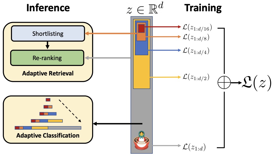
Core Idea
-
A conventional embedding model learns a representation:
\[z = F(x;\theta_F) \in \mathbb{R}^{d}\]-
where all \(d\) dimensions are typically used together. MRL changes the learning problem so that multiple prefixes of the same vector are trained to solve the same task. If \(\mathcal{M} \subset [d]\) is the set of chosen nesting sizes, then each prefix:
\[z_{1:m} = F(x;\theta_F)_{1:m}, \quad m \in \mathcal{M}\]- is encouraged to be a complete representation at its own scale. Matryoshka Representation Learning by Kusupati et al. (2022) emphasizes that only \(O(\log d)\) nesting sizes need to be explicitly optimized, while intermediate dimensions often interpolate smoothly in accuracy.
-
-
In supervised classification, the MRL objective can be written as:
\[\min_{\theta_F,\{W^{(m)}\}_{m \in \mathcal{M}}} \frac{1}{N} \sum_{i=1}^{N} \sum_{m \in \mathcal{M}} c_m \mathcal{L} \left( W^{(m)} F(x_i;\theta_F)_{1:m}, y_i \right)\]- where \(W^{(m)} \in \mathbb{R}^{L \times m}\) is a classifier for the \(m\)-dimensional prefix, \(c_m \ge 0\) weights the importance of each nesting size, and \(\mathcal{L}\) is typically cross-entropy. Efficient MRL ties classifier weights across dimensions with \(W^{(m)} = W_{:,1:m}\), reducing classifier overhead while preserving the nested training signal. Matryoshka Representation Learning by Kusupati et al. (2022) introduces this efficient variant as MRL-E.
Prefix Ordering
- The ordering constraint is the key design choice. MRL does not merely compress a vector after training; it trains the model so that earlier coordinates carry broad, high-value information and later coordinates refine that information. This turns the embedding into a sequence of increasingly detailed views:
- This is different from post-hoc dimensionality reduction, random feature selection, or training multiple unrelated low-dimensional models. Post-hoc compression can reduce storage, but it does not guarantee that the first coordinates of the original embedding are semantically useful; MRL makes this property part of the training objective. Matryoshka Representation Learning by Kusupati et al. (2022) compares MRL against fixed-feature models, SVD, random feature selection, and slimmable networks, showing that MRL is consistently strong across representation sizes.
Relationship to Representation Learning
-
MRL is best understood as a wrapper around existing representation learning objectives rather than a new backbone architecture. It can be applied to supervised vision models, masked language models, and contrastive vision-language models because it only requires evaluating the training objective at several prefixes of the representation. BERT by Devlin et al. (2018) introduced masked language modeling for bidirectional text representations, and Matryoshka Representation Learning by Kusupati et al. (2022) shows that the MRL idea can be adapted to BERT-style language representations.
-
For vision-language contrastive learning, MRL can be applied to both sides of the contrastive pair. If image and text encoders produce normalized embeddings \(u_i\) and \(v_i\), then the contrastive loss can be evaluated at each nesting size:
\[\mathcal{L}_{\mathrm{MRL}} = \sum_{m \in \mathcal{M}} c_m \left( \mathcal{L}_{I \rightarrow T}^{(m)} + \mathcal{L}_{T \rightarrow I}^{(m)} \right)\]- where each term uses \(u_{1:m}\) and \(v_{1:m}\) after size-specific normalization. CLIP by Radford et al. (2021) learns visual concepts from image-text contrastive supervision, ALIGN by Jia et al. (2021) scales contrastive vision-language learning with noisy alt-text data, and Matryoshka Representation Learning by Kusupati et al. (2022) extends the Matryoshka objective to ALIGN-style vision-language embeddings.
Adaptive Retrieval
- Retrieval is one of the most natural uses of MRL because search cost scales with embedding dimensionality. A standard exact nearest-neighbor search over \(N\) database vectors costs approximately \(O(Nd)\) per query. With MRL, a system can first shortlist candidates using a small prefix \(d_s\) and then re-rank only a smaller set using a larger prefix \(d_r\):
-
This creates a funnel: cheap low-dimensional search narrows the candidate set, and higher-dimensional representations are reserved for harder ranking decisions. Matryoshka Representation Learning by Kusupati et al. (2022) reports up to 14x real-world speed-ups for large-scale retrieval while maintaining comparable retrieval quality.
-
The following figure (source) shows the adaptive retrieval trade-off between mAP@10 and MFLOPs per query, where Matryoshka adaptive retrieval lies above the fixed-dimensional single-shot retrieval Pareto frontier.
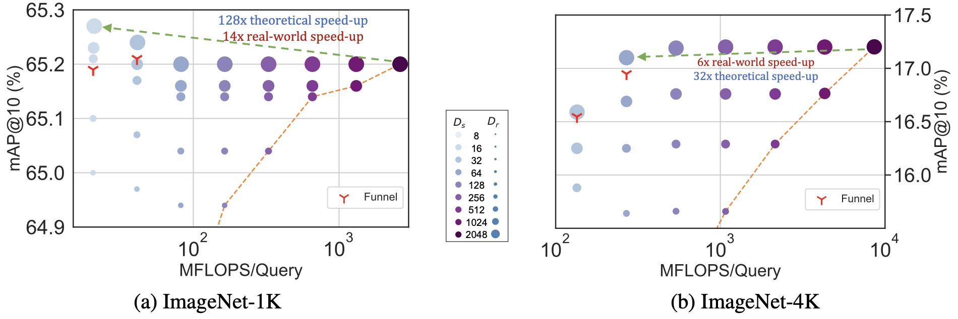
Adaptive Classification
- MRL also enables adaptive classification cascades without running multiple neural networks. A classifier can first evaluate a low-dimensional prefix; if confidence is high, prediction stops early, and if confidence is low, the classifier uses a larger prefix. This gives a per-example accuracy-cost trade-off:
-
Matryoshka Representation Learning by Kusupati et al. (2022) shows that adaptive classification with MRL can match a 512-dimensional fixed-feature classifier on ImageNet-1K while using an expected dimensionality of roughly 37 dimensions, corresponding to about a 14x smaller representation for the same accuracy level.
-
The following figure (source) shows adaptive classification with MRL ResNet50, where cascaded prefixes achieve the same accuracy with much smaller expected representation size.
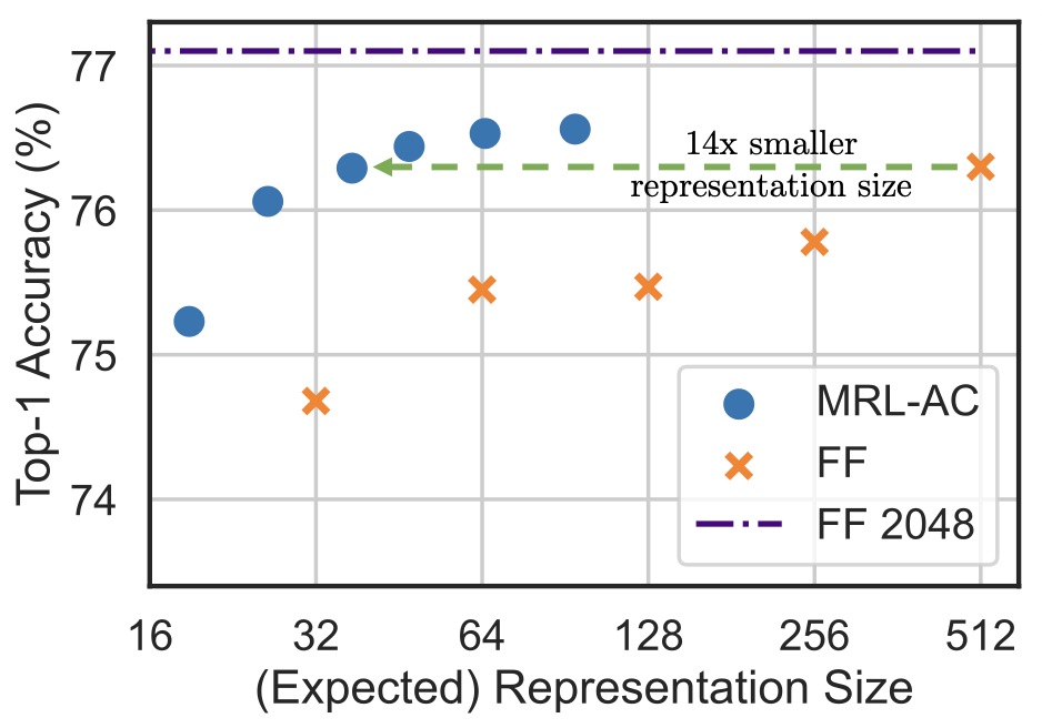
OpenAI Embeddings and Truncation
-
The practical significance of MRL became especially visible in modern embedding APIs. New embedding models and API updates explains that OpenAI’s newer embedding models were trained with a technique that permits shortening embeddings by removing trailing dimensions, and it gives the example that
text-embedding-3-largeshortened to 256 dimensions can still outperform an unshortened 1536-dimensionaltext-embedding-ada-002embedding on MTEB. -
This is the production version of the Matryoshka principle: a developer can choose a dimensionality based on the vector database limit, storage budget, latency constraint, or target recall. For example, a high-recall semantic search system may store 1024 or 3072 dimensions, while a cost-sensitive classification or clustering pipeline may store 256 dimensions. New embedding models and API updates explicitly describes this as a performance-cost trade-off exposed through the
dimensionsAPI parameter.
Multimodal Matryoshka Learning
-
Multimodal Matryoshka (M3) learning extends the same nested-capacity idea beyond embedding dimensions. In large multimodal models, the bottleneck is often not the width of a single embedding vector, but the number of visual tokens passed into the language model. Matryoshka Multimodal Models by Cai et al. (2024) adapts the Matryoshka idea to token length, learning nested sets of visual tokens that represent an image at progressively finer granularities.
-
The distinction is important:
-
In standard MRL, elasticity is created across embedding dimensions; in multimodal M3, elasticity is created across visual token counts. Both variants allow a single model to serve multiple accuracy-cost operating points, but they apply the nesting principle to different bottlenecks: vector width for representation systems and token length for multimodal reasoning systems.
-
In a model such as LLaVA, an image encoder commonly produces a grid of visual tokens that are fed as prefix tokens to an LLM. Visual Instruction Tuning by Liu et al. (2023) introduced LLaVA as a multimodal assistant connecting a vision encoder and language model through visual instruction tuning, while Matryoshka Multimodal Models by Cai et al. (2024) modifies this setting so the model can choose among nested token granularities at inference time.
-
The following figure (source) shows M3, where coarser visual token sets are derived from finer token sets and image descriptions become more detailed as the token granularity increases.
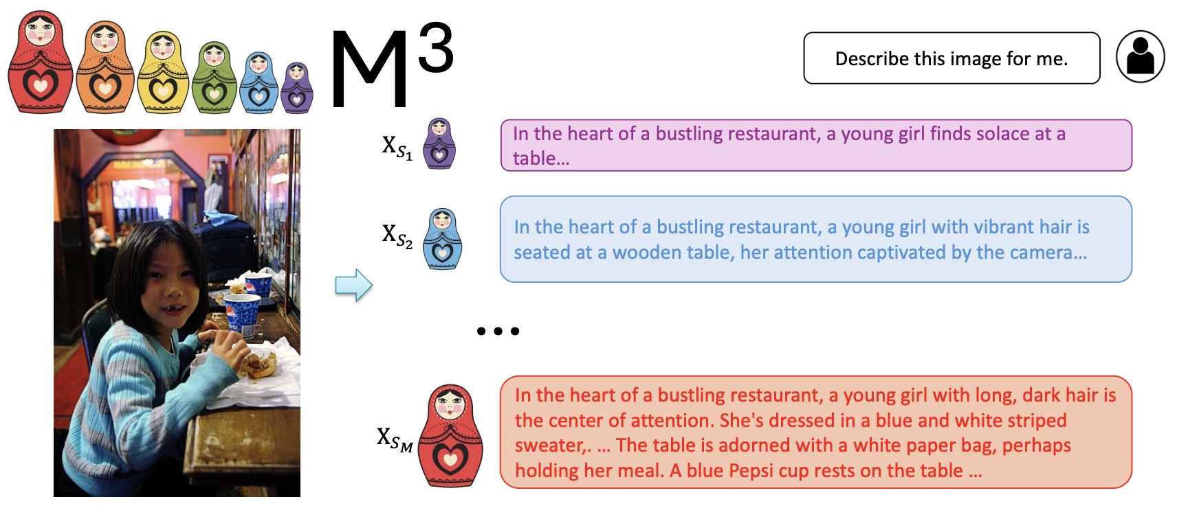
Token-Level Nesting in Matryoshka Multimodal Models
- For an image \(I\), a vision encoder such as CLIP-ViT can produce an \(H \times W\) grid of visual tokens:
-
M3 constructs a hierarchy of token sets:
\[X_{S_1}, X_{S_2}, \ldots, X_{S_M}, \quad |S_1| < |S_2| < \cdots < |S_M|\]- with the nesting constraint:
-
For CLIP-ViT-L-336, the full grid contains \(24 \times 24 = 576\) visual tokens; Matryoshka Multimodal Models by Cai et al. (2024) uses pooled scales such as \(\{1,9,36,144,576\}\), where coarser tokens preserve global semantics and larger token sets add local detail.
-
The following figure (source) shows the architecture of Matryoshka Multimodal Models, where CLIP visual features are organized into coarse-to-fine visual token groups and a granularity controller selects how many tokens the LLM receives. At test time, users can thus explicitly control the granularity of the visual features with M3.
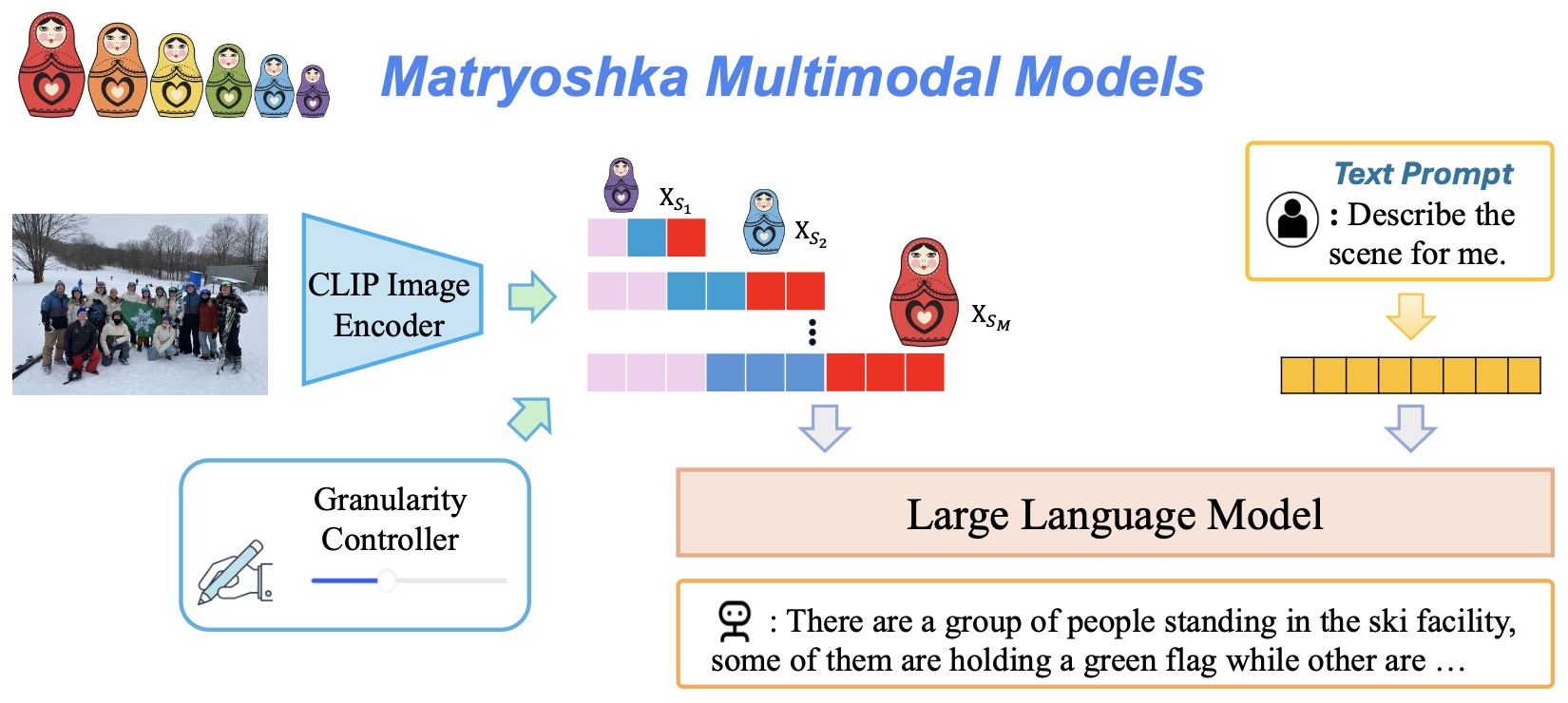
Multimodal Training Objective
- M3 trains the multimodal model to answer correctly at every visual token scale. Given question tokens \(X_q\), answer tokens \(X_a = (x_1,\ldots,x_L)\), and a visual token set \(X_{S_i}\), the autoregressive likelihood is:
- The final training objective averages the negative log-likelihood across all token scales:
- This objective teaches the same LMM to operate with sparse global visual information or dense fine-grained visual information. Matryoshka Multimodal Models by Cai et al. (2024) reports that the model does not require new learnable architectural components for the hierarchy; instead, the image encoder and LMM are optimized to make the nested visual token sets useful.
Token Efficiency
-
The cost of transformer attention grows with sequence length, so reducing visual tokens can produce large savings in multimodal inference. Linformer by Wang et al. (2020) and Reformer by Kitaev et al. (2020) address long-sequence inefficiency through attention approximations, while Token Merging by Bolya et al. (2022) reduces ViT computation by merging similar tokens.
-
M3 differs from ordinary token reduction because it does not produce a single reduced token length. Instead, it trains a single model to expose multiple token budgets at inference time. This allows a system to spend few visual tokens on simple images, more visual tokens on OCR-heavy or document-like images, and potentially different budgets across frames in video. Matryoshka Multimodal Models by Cai et al. (2024) finds that COCO-style benchmarks can often be handled with around 9 visual tokens, while OCR and document-understanding tasks require substantially more tokens.
Granularity vs. Difficulty
-
A useful interpretation of MRL and M3 is that representation scale becomes a diagnostic signal. If a sample is correctly classified or answered with a small prefix or a small token set, it may be visually or semantically simple. If correctness requires the full representation, the example likely depends on fine details, rare distinctions, text in the image, or visually dense context. Matryoshka Representation Learning by Kusupati et al. (2022) uses disagreement across dimensions to analyze difficulty and semantic hierarchy, and Matryoshka Multimodal Models by Cai et al. (2024) uses token-scale behavior to study image complexity in multimodal benchmarks.
-
The following figure (source) shows TextVQA samples where answers vary across visual token scales, illustrating how token granularity can act as a proxy for image and question complexity.
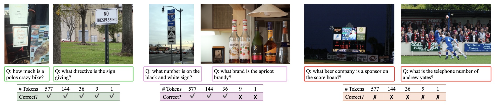
Deployment Guidance
-
For embedding systems, Matryoshka training is most useful when the same semantic representation must serve several budgets: small mobile indexes, medium-size retrieval systems, and high-recall server-side ranking. A common pattern is to store a shorter prefix for the first retrieval stage and use longer prefixes for reranking. RAIVNLab/MRL provides code for training, evaluating, and analyzing Matryoshka representations with a ResNet50 backbone.
-
For multimodal systems, token-level Matryoshka learning is most useful when the number of visual tokens dominates inference cost. High-resolution images, videos, charts, documents, and OCR-heavy inputs can require more visual detail, while ordinary scene-level question answering may need far fewer tokens. Matryoshka Multimodal Models by Cai et al. (2024) demonstrates this principle by training LLaVA-style models with nested visual token scales.
-
The unifying practical rule is to match representation capacity to the difficulty of the instance and the constraints of the deployment environment: use fewer dimensions or fewer visual tokens when the task is simple or latency-sensitive, and expand to richer representations when the query, image, video, or downstream decision requires more detail. This principle sets up the next class of modern embedding systems: lightweight and LLM-derived embedding models that treat efficiency, dimensional flexibility, and deployment cost as first-class design goals.
Transition to LLM-Derived Embeddings
-
The next stage in the evolution of embeddings involves tightly integrating them with LLMs. Instead of training embeddings independently, modern systems:
- Initialize from pretrained LLM weights
- Adapt architectures to improve bidirectional understanding
- Use distillation and large-scale data curation pipelines
-
This transition reflects a deeper shift: embedding models are no longer separate components but specialized views of general-purpose intelligence systems.
-
The following sections examine this paradigm in detail, beginning with EmbeddingGemma and its design as a lightweight yet high-performance embedding model derived from LLM architectures.
LLM-Derived Embedding Models
-
The emergence of Large Language Models (LLMs) has fundamentally changed how embedding systems are built. Earlier embedding models were typically trained directly on manually curated retrieval, classification, or similarity datasets. Modern systems increasingly leverage LLMs as sources of knowledge, supervision, architectural initialization, or even as the embedding model itself. This evolution has produced several distinct approaches to embedding model construction, each addressing the same underlying challenge: how to transform the rich semantic knowledge contained within generative foundation models into compact, reusable vector representations.
-
Four major paradigms have emerged:
- Lightweight LLM-derived encoder construction adapts knowledge from a pretrained LLM family into a compact embedding model, emphasizing efficient inference, small memory footprint, dimensional flexibility, and strong performance under deployment constraints rather than only maximizing benchmark accuracy through scale.
- Data-centric distillation uses an LLM as a teacher, data generator, and relevance annotator, allowing a smaller embedding model to learn from synthetic queries, task descriptions, positives, and hard negatives rather than from human-labeled data alone.
- Architecture-centric adaptation modifies the generative LLM itself, typically by changing a causal decoder into a bidirectional encoder and then training it with objectives that make its hidden states useful for retrieval and similarity.
- Foundation-model embedding projection trains embeddings directly on top of foundation models that already possess broad language or multimodal understanding, making the embedding model a specialized projection of a larger representation system.
-
EmbeddingGemma: Powerful and Lightweight Text Representations by Vera et al. (2025), Gecko: Versatile Text Embeddings Distilled from Large Language Models by Lee et al. (2024), LLM2Vec: Large Language Models Are Secretly Powerful Text Encoders by BehnamGhader et al. (2024), BidirLM: From Text to Omnimodal Bidirectional Encoders by Adapting and Composing Causal LLMs by Boizard et al. (2026), and Gemini Embedding: Generalizable Embeddings from Gemini by Lee et al. (2025) represent successive milestones within the LLM-derived embedding trajectory. Together, they illustrate the transition from compact LLM-initialized text encoders and synthetic-data-driven retrievers to adapted decoder-based encoders and foundation-model-derived embedding systems.
-
Gemini Embedding 2: A Native Multimodal Embedding Model from Gemini by Shanbhogue et al. (2026) is related to this trajectory because it builds on Gemini’s foundation-model capabilities, but it is best positioned in the subsequent native multimodal and omnimodal embeddings section rather than treated primarily as an LLM-derived text embedding model. Its role in the primer is to mark the transition from LLM-derived text and encoder adaptation methods toward native multimodal embedding systems capable of encoding text, images, audio, video, documents, and mixed-modality inputs within a common semantic space.
EmbeddingGemma: Lightweight General-Purpose Text Embeddings
- EmbeddingGemma represents a critical step in reconciling two competing goals in modern embedding systems: maximizing semantic performance while minimizing computational cost. Unlike earlier approaches that scaled model size to improve quality, EmbeddingGemma demonstrates that careful architectural design, training strategies, and knowledge distillation can produce compact models that rival much larger systems.
Architecture
- EmbeddingGemma demonstrates that high-quality embeddings can be achieved without scaling model size. It combines encoder adaptation from LLMs, contrastive and distillation objectives, geometry-aware regularization, and deployment-focused optimizations to produce a compact yet general-purpose embedding system.
- This section details how these components interact to form a performant and efficient embedding model.
Encoder Construction from Decoder LLMs
-
A central design decision in EmbeddingGemma is transforming a decoder-only LLM into a representation-focused encoder. Decoder models are trained with causal masking, where each token attends only to preceding tokens. This is suboptimal for embeddings, where full-context understanding is required.
-
To address this, EmbeddingGemma first adapts a pretrained Gemma model into an encoder-decoder architecture using a denoising objective. The encoder component is then extracted and used as the embedding backbone .
-
This approach aligns with Exploring the Limits of Transfer Learning with a Unified Text-to-Text Transformer (T5) by Raffel et al. (2020), where encoder-decoder models enable specialization of the encoder for input understanding.
-
Formally, for an input sequence:
\[T = (t_1, t_2, \dots, t_L)\]-
the encoder produces contextual representations:
\[H = \text{Encoder}(T) \in \mathbb{R}^{L \times d}\]
-
-
These representations encode bidirectional context, allowing each token to incorporate information from the entire sequence.
Pooling and Embedding Projection
-
To obtain a fixed-length embedding, token representations are aggregated:
\[z = P(H)\]-
where \(P(\cdot)\) is typically mean pooling. Mean pooling is preferred due to:
- Stability across varying sequence lengths
- Minimal additional parameters
- Strong empirical performance in retrieval settings
-
-
The pooled vector is then projected into the embedding space:
-
EmbeddingGemma employs a hierarchical projection:
- Internal representation space (higher dimensional, e.g., 3072)
- Final embedding space (e.g., 768 or smaller truncated forms)
-
This structure enables both expressive representations and efficient deployment.
Contrastive Training with Hard Negatives
-
The primary training signal is contrastive learning. The model is trained on triples:
- Query \(q\)
- Positive document \(p^+\)
- Negative documents \(p^-\)
-
The objective maximizes similarity between \(q\) and \(p^+\) while minimizing similarity to negatives:
- Hard negatives are critical. These are semantically similar but incorrect examples, forcing the model to learn fine-grained distinctions. This principle is well-established in Dense Passage Retrieval by Karpukhin et al. (2020), which showed that hard negatives significantly improve retrieval quality.
Geometric Embedding Distillation
- EmbeddingGemma inherits knowledge from a stronger embedding model through geometric distillation. Instead of only learning relative similarities, it aligns its embeddings with those of a teacher model:
-
This preserves global structure in the embedding space. The teacher model, derived from Gemini-based embeddings, provides a high-quality geometric reference .
-
This approach ensures that the compact model retains semantic relationships learned by larger systems.
Spread-Out Regularization and Embedding Geometry
-
Embedding spaces often suffer from anisotropy, where vectors cluster in narrow regions. This reduces effective dimensionality and harms retrieval.
-
EmbeddingGemma introduces a spread-out regularizer:
-
This encourages embeddings to be uniformly distributed, improving:
- Retrieval diversity
- Nearest-neighbor search quality
- Robustness under compression
-
This addresses issues identified in On the Sentence Embeddings from Pre-trained Language Models by Ethayarajh (2019), where embedding anisotropy limits representational effectiveness.
Model Souping for Generalization
- EmbeddingGemma uses model souping to combine multiple fine-tuned models:
-
Each model is trained on different mixtures of tasks and domains. Averaging weights produces a model that generalizes better across tasks without increasing inference cost.
-
This technique originates from Model soups by Wortsman et al. (2022), which showed that weight averaging can outperform selecting a single checkpoint.
Efficiency Mechanisms
-
A distinguishing feature of EmbeddingGemma is that efficiency is treated as a primary design objective rather than a post-training optimization. Traditional embedding systems often train a large, fixed-dimensional representation and later compress it through dimensionality reduction or quantization. These post hoc approaches can degrade retrieval quality and semantic fidelity.
-
EmbeddingGemma instead incorporates efficiency directly into training through two complementary techniques: Matryoshka Representation Learning and quantization-aware optimization. Together, these techniques allow the model to operate across environments ranging from large-scale cloud retrieval systems to memory-constrained edge devices.
-
Matryoshka representations and quantization address two distinct sources of cost:
- Matryoshka Representation Learning compresses embedding vectors, reducing vector index size and retrieval latency
- Quantization compresses model weights, reducing inference memory and serving cost
-
Together, they enable EmbeddingGemma to support a wide range of deployment scenarios using a single model. It can produce embeddings at multiple dimensionalities, operate efficiently on constrained hardware, support large-scale retrieval workloads, and maintain competitive quality under aggressive compression.
-
This combination is a major reason EmbeddingGemma is particularly attractive for production retrieval systems, edge deployment, and large-scale RAG architectures, where both inference efficiency and vector storage costs are critical.
Matryoshka Representation Learning
-
Conventional embedding models produce vectors with a fixed dimensionality. For example, a 768-dimensional embedding model requires every downstream application to store and index all 768 dimensions, regardless of the application’s quality, latency, or storage requirements. A detailed discourse of this technique has been offered in the Matryoshka Representation Learning: Adaptive and Elastic Embeddings section.
-
MRL, introduced in Matryoshka Representation Learning by Kusupati et al. (2022), organizes information hierarchically within the embedding vector. Earlier dimensions contain the most important semantic information, while later dimensions progressively refine the representation.
-
Formally, given a full embedding \(e \in \mathbb{R}^{d}\), a truncated embedding is:
\[e^{(k)} = e_{1:k}\]-
where:
\[k < d\]
-
-
The key property is that \(e^{(k)}\) remains a valid embedding even when later dimensions are removed.
-
Rather than optimizing only the full vector, MRL optimizes multiple nested representations simultaneously:
-
This means the first 128 dimensions are trained to function as a standalone embedding, the first 256 dimensions form a stronger embedding, and so on.
-
This provides several practical benefits:
- Storage requirements can be adjusted without retraining
- Retrieval systems can trade quality for efficiency dynamically
- Vector database memory consumption can be significantly reduced
- Query latency decreases because fewer dimensions must be processed
-
For a corpus containing \(N\) vectors, storage scales approximately as:
-
Reducing dimensionality from 768 to 128 lowers storage requirements by:
\[\frac{128}{768} = \frac{1}{6}\]- while often retaining much of the retrieval quality.
####### Retrieval Trade-Offs
-
Retrieval systems typically operate under competing constraints: higher-dimensional vectors tend to improve retrieval quality, while lower-dimensional vectors improve latency and memory efficiency. Traditional embedding models require selecting one operating point during training. MRL removes this constraint by allowing a single model to support multiple deployment configurations.
-
Common configurations include:
- 3072 dimensions: maximum-quality retrieval for high-recall production systems
- 1536 dimensions: strong-quality retrieval with lower storage cost
- 768 dimensions: general-purpose RAG and semantic search
- 256 dimensions: mobile or latency-sensitive retrieval
- 128 dimensions: on-device semantic search and compact local indexes
-
This flexibility is especially important in modern Retrieval-Augmented Generation systems, where large corpora may require billions of stored vectors.
Quantization
-
While dimensionality reduction decreases vector storage, model inference remains expensive unless model weights are also compressed. Quantization addresses this by representing parameters with lower-precision numerical formats.
-
A standard transformer may store weights using \(16\text{-bit}\) or \(32\text{-bit}\) floating-point values. Quantized models instead represent parameters using \(8\text{-bit}\) or even \(4\text{-bit}\) integers.
-
The approximate memory reduction is:
\[\text{Compression Ratio} =\frac{\text{Original Precision}} {\text{Quantized Precision}}\]- For example, \(\frac{16}{4} = 4\times\), meaning a 4-bit model can require roughly one-quarter of the memory footprint of a 16-bit model.
-
Unlike many embedding systems that are quantized only after training, EmbeddingGemma is designed to remain robust under aggressive quantization, retaining strong performance even with reduced numerical precision.
####### Advantages
-
Quantization provides several deployment advantages:
- Reduced memory footprint: smaller models can fit more easily into GPU, CPU, or mobile memory
- Higher throughput: lower-precision arithmetic allows more embeddings to be generated per second
- Lower inference latency: reduced memory bandwidth and improved hardware utilization speed up responses
- Lower serving cost: reduced compute and memory requirements decrease infrastructure costs
Retrieval Implications
-
EmbeddingGemma is particularly effective in large-scale retrieval pipelines.
-
Given a query \(q\) and corpus \(\mathcal{C}\):
-
Its advantages include:
- Low latency due to compact architecture
- Reduced storage via dimensional truncation
- Strong cross-domain generalization
-
These properties make it suitable for:
- Retrieval-Augmented Generation systems
- Semantic search engines
- On-device retrieval applications
Gecko: Data-Centric Distillation from Large Language Models
Motivation
-
A recurring challenge in embedding model development is data quality. High-performing retrieval systems require large collections of query-document pairs, relevance labels, and hard negatives. Constructing such datasets manually is expensive, domain-limited, and often fails to capture the diversity of real-world information needs.
-
Gecko: Versatile Text Embeddings Distilled from Large Language Models by Lee et al. (2024) addresses this problem through a data-centric distillation strategy. Rather than adapting the LLM architecture itself, Gecko uses an LLM as a teacher that generates retrieval supervision for a compact embedding model. The core insight is that a sufficiently capable LLM already possesses broad world knowledge and task understanding, making it possible to synthesize high-quality retrieval datasets directly from unlabeled corpora.
-
This approach shifts the focus from model architecture to training signal quality. The embedding model remains relatively compact, while the LLM acts as a scalable source of supervision.
The FRet Retrieval Dataset
-
Gecko introduces FRet, a large retrieval-oriented training corpus automatically generated using LLMs.
-
Given an unlabeled passage \(p_i\), an LLM generates a structured training example that includes a task instruction, a natural-language query, and an initial source passage:
\[(t_i, q_i, p_i)\]-
where:
-
\(t_i\) denotes the task instruction that describes the intended retrieval behavior.
-
\(q_i\) denotes the generated query that expresses a realistic information need.
-
\(p_i\) denotes the source passage from which the initial synthetic query-task pair was derived.
-
-
-
The generated query is not merely a paraphrase of the passage. Instead, the LLM is prompted to produce realistic information-seeking questions that could plausibly retrieve the passage. This creates retrieval supervision without requiring human annotation.
Synthetic Query and Task Generation
-
A key innovation in Gecko is the explicit generation of both task descriptions and queries.
-
Traditional retrieval datasets often assume a fixed retrieval objective. Gecko instead exposes the model to a diverse range of retrieval tasks, including question answering, fact retrieval, semantic matching, information extraction, and classification-oriented retrieval. This task diversity improves generalization across downstream benchmarks and allows a single embedding model to support many retrieval settings.
-
Conceptually, the generated query distribution approximates:
\[q \sim P(q \mid p)\]- where the LLM serves as an approximation to the latent distribution of plausible information needs associated with passage \(p\).
Retrieval-Based Candidate Mining
-
After generating a query, Gecko performs retrieval using an existing embedding model.
-
For each query \(q_i\), a candidate set of passages is retrieved:
\[\mathcal{C}_i ={p_1,p_2,\dots,p_k}\] -
Importantly, the original source passage is not automatically assumed to be the best answer.
-
Gecko observes that generated queries frequently correspond more closely to neighboring passages than to the passage from which the query originated. Consequently, additional filtering is required.
LLM-Based Positive and Hard-Negative Relabeling
-
Gecko’s second major contribution is LLM-based reranking and relabeling.
-
The retrieved candidate set is presented back to the LLM, which identifies the strongest positive passage and semantically close but incorrect hard negatives, producing a higher-quality contrastive training example than the original synthetic pair alone.
-
This results in triples:
\[(q_i,p_i^+,p_i^-)\]-
where:
-
\(p_i^+\) is the passage selected by the LLM as the best positive match for the generated query.
-
\(p_i^-\) is a semantically similar but incorrect passage selected to function as a hard negative during contrastive training.
-
This relabeling step is critical because it improves supervision quality beyond simple nearest-neighbor retrieval.
-
The resulting dataset better reflects retrieval difficulty and creates informative negative examples that strengthen contrastive learning.
-
-
-
The following figure (source) shows the Gecko training pipeline, where an LLM generates task-query pairs and mines positive and negative passages to construct the FRet retrieval corpus.
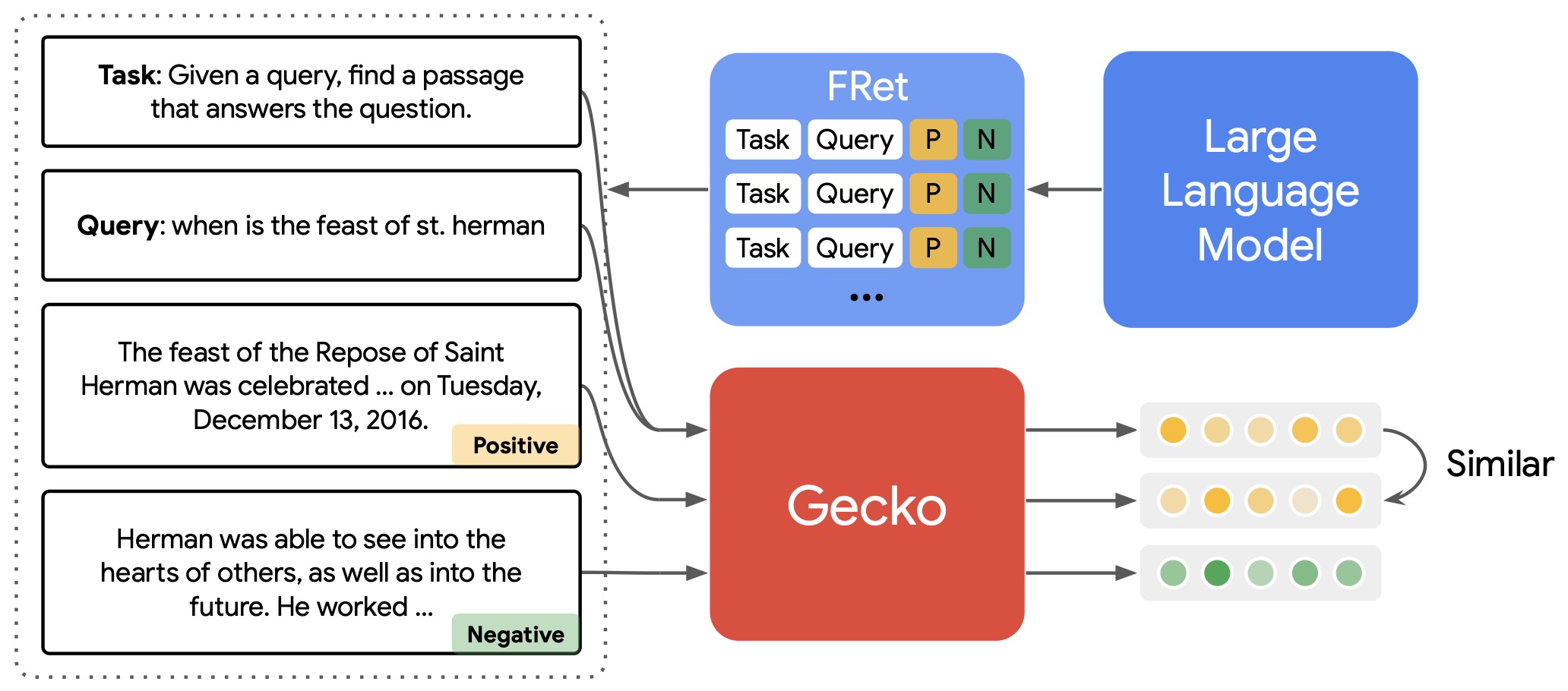
Contrastive Retriever Training
-
Once FRet has been constructed, Gecko trains a dual-encoder retrieval model using contrastive learning.
-
For a query embedding \(q\) and positive passage embedding \(p^{+}\), the objective maximizes similarity between matching pairs while separating negatives.
-
The contrastive objective follows an InfoNCE formulation:
\[\mathcal{L}_{\text{contrastive}} =-\log \frac{ \exp(\mathrm{sim}(q,\mathbf{p}^{+})/\tau) }{ \sum_j \exp(\mathrm{sim}(q,\mathbf{p}_j)/\tau) }\]-
where:
-
\(\tau\) is a temperature parameter controlling how sharply the model distinguishes positive passages from competing candidates.
-
\(\mathbf{p}_j\) ranges over the positive passage, hard negatives, and other in-batch candidate passages used to define the retrieval distribution.
-
-
-
This objective aligns retrieval-relevant semantics within the embedding space and enables efficient nearest-neighbor search.
Why Gecko Works
-
Gecko can be interpreted as a large-scale knowledge distillation system.
-
Rather than directly compressing model parameters, it compresses the LLM’s world knowledge, retrieval behavior, task understanding, and relevance judgments into a retrieval dataset that can train a smaller embedding model.
-
The LLM serves multiple roles during dataset construction: it generates plausible queries, supplies task framing, judges candidate passages, and mines hard negatives that make the final contrastive training signal more informative.
-
Consequently, a relatively small encoder can inherit retrieval capabilities that would otherwise require significantly larger models.
Strengths and Limitations
-
Strengths:
- Gecko does not require architectural modification of the retriever, making it compatible with standard dual-encoder retrieval pipelines.
- Gecko scales with unlabeled corpora because supervision is synthesized from raw passages rather than collected through manual annotation.
- Gecko produces diverse retrieval supervision by generating both task descriptions and queries, rather than only query-document pairs.
- Gecko achieves strong retrieval performance despite compact model size because the LLM is used where it is most valuable: constructing supervision before training rather than serving at inference time.
- Gecko demonstrates strong parameter-efficiency on MTEB-style benchmarks, including results where lower-dimensional Gecko embeddings remain competitive with larger embedding systems.
-
Limitations:
- Gecko transfers knowledge indirectly through data rather than by reusing internal LLM representations.
- Gecko’s final performance depends heavily on the quality, diversity, and calibration of synthetic data produced by the teacher LLM.
- Gecko cannot directly inherit the hidden-state geometry of the LLM because the generative model remains external to the retriever.
- Gecko requires computationally expensive LLM generation and relabeling during dataset construction, even though inference with the final retriever is efficient.
Gecko in the Broader Evolution of Embeddings
-
Gecko established one of the first successful demonstrations that LLMs could substantially improve embedding models without being converted into embedding models themselves.
-
This data-centric perspective influenced later systems, including Gemini Embedding: Generalizable Embeddings from Gemini by Lee et al. (2025), which similarly leverages Gemini-derived supervision and broad-domain knowledge transfer, and EmbeddingGemma: Powerful and Lightweight Text Representations by Vera et al. (2025), which combines geometric distillation and encoder initialization to transfer knowledge from larger models into compact embedding architectures.
-
At the same time, Gecko highlights a limitation of purely data-centric approaches: the generative model remains external to the embedding system. Subsequent work explored whether the LLM itself could become the encoder, leading to architecture-centric approaches such as LLM2Vec and BidirLM.
LLM2Vec: Decoder-to-Encoder Adaptation
-
LLM2Vec provides an architecture-centric answer to the same broad problem addressed by Gecko: how to transfer the semantic knowledge of generative LLMs into embedding systems. Unlike Gecko, which keeps the LLM external and uses it to generate retrieval supervision, LLM2Vec modifies the decoder-only LLM itself so that it can function as a text encoder. LLM2Vec: Large Language Models Are Secretly Powerful Text Encoders by BehnamGhader et al. (2024) introduces this as an unsupervised recipe for transforming decoder-only LLMs into universal text encoders.
-
LLM2Vec is important because decoder-only LLMs already contain broad linguistic, factual, and instruction-following knowledge, but their causal attention pattern is not naturally suited to embedding tasks. The method shows that a relatively lightweight adaptation procedure can expose this latent encoder capability without requiring synthetic GPT-4-style data generation or full retraining from scratch. LLM2Vec: Large Language Models Are Secretly Powerful Text Encoders by BehnamGhader et al. (2024) evaluates this recipe on decoder-only models ranging from 1.3B to 8B parameters and reports strong results on word-level and sequence-level embedding tasks.
Motivation
-
Text embedding models require representations that summarize an entire input sequence. For retrieval, semantic similarity, clustering, and classification, the model must encode the full meaning of a sentence, passage, or document into a fixed vector representation.
-
Decoder-only LLMs are strong generative models, but they are trained with causal attention. This means each token representation is conditioned only on tokens to its left. This is appropriate for next-token prediction, but it prevents intermediate token states from using information from future tokens, which is a disadvantage for encoding complete input sequences.
-
The central motivation of LLM2Vec is therefore to preserve the knowledge and ecosystem advantages of decoder-only LLMs while removing the architectural constraint that prevents them from acting as strong bidirectional text encoders.
Why Causal LLMs Are Poor Encoders by Default
- A decoder-only LLM models a sequence autoregressively:
-
This objective is excellent for generation because it trains the model to predict the next token using previous context. However, embeddings require a different kind of representation: the vector for a sentence or passage should reflect information from the entire input, not only a left-to-right prefix.
-
Under causal attention, the hidden state at position \(i\) can attend only to earlier positions:
- A bidirectional encoder instead allows each token representation to use all positions in the input sequence:
- This difference is central to why encoder-only models such as BERT by Devlin et al. (2018) historically performed well on representation tasks, while decoder-only models required adaptation before being competitive as text encoders.
The Three-Step LLM2Vec Recipe
-
LLM2Vec transforms a decoder-only LLM into a text encoder through three stages: first, enabling bidirectional attention; second, adapting the model with masked next-token prediction; and third, applying unsupervised contrastive learning to improve sequence-level embeddings. LLM2Vec: Large Language Models Are Secretly Powerful Text Encoders by BehnamGhader et al. (2024) presents this pipeline as a simple, unsupervised, and parameter-efficient conversion method.
-
The following figure (source) shows the three-stage LLM2Vec adaptation pipeline consisting of bidirectional attention, masked next-token prediction, and unsupervised contrastive learning.
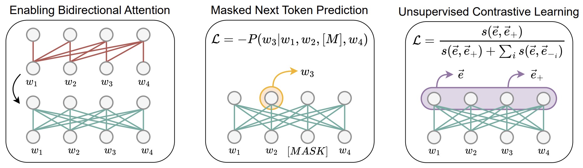
- The key contribution is not any single step in isolation. Rather, LLM2Vec demonstrates that decoder-only LLMs require both an attention-level change and an objective-level adaptation before their representations become suitable for embedding tasks.
Enabling Bidirectional Attention
-
The first step changes the attention mask. In a causal model, attention is restricted by a lower-triangular mask, so token \(x_i\) cannot attend to tokens \(x_j\) where \(j > i\). LLM2Vec removes this constraint and enables every token to attend to every other token.
-
This converts the hidden-state computation from a causal form:
\[h_i = f_\theta(x_{\leq i})\]-
to a bidirectional form:
\[h_i = f_\theta(x_1, x_2, \dots, x_T)\]
-
-
This attention change is necessary but not sufficient. The model’s parameters were originally optimized under causal masking, so the model does not automatically know how to use right-context information effectively. This is why LLM2Vec introduces a second adaptation step rather than stopping at the attention-mask change.
Masked Next-Token Prediction
-
The second step is masked next-token prediction, which teaches the converted model how to use bidirectional context while remaining close to the original next-token prediction structure. Given an input sequence \(x=(x_1,\dots,x_T)\) and a set of masked positions \(M\), the model is trained to reconstruct masked content using both left and right context.
-
A simplified objective can be written as:
-
The purpose of this phase is not primarily to optimize retrieval performance. Instead, it repairs the mismatch between the model’s original causal training regime and the newly enabled bidirectional attention pattern.
-
LLM2Vec is careful to preserve the decoder-style next-token-prediction structure while allowing future context to influence hidden states. This makes masked next-token prediction a bridge between autoregressive pretraining and encoder-style representation learning. LLM2Vec: Large Language Models Are Secretly Powerful Text Encoders by BehnamGhader et al. (2024) identifies this step as essential for adapting decoder-only LLMs into strong text encoders.
Unsupervised Contrastive Learning
-
The third step applies unsupervised contrastive learning to improve sequence-level representations. After bidirectional attention and masked next-token prediction produce richer contextual token states, contrastive learning shapes the global embedding space so semantically similar inputs are closer and unrelated inputs are farther apart.
-
LLM2Vec follows the SimCSE-style formulation, where the same sentence is passed through the model twice with independent dropout masks. The two resulting embeddings act as positive views of the same input, while other examples in the batch serve as negatives. SimCSE: Simple Contrastive Learning of Sentence Embeddings by Gao et al. (2021) introduced this dropout-based unsupervised contrastive framework for sentence embeddings.
-
A simplified SimCSE-style loss is:
\[\mathcal{L}_{\text{SimCSE}} =-\log \frac{ \exp(\mathrm{sim}(\mathbf{z}_i,\mathbf{z}_i^+)/\tau) }{ \sum_{j=1}^{B} \exp(\mathrm{sim}(\mathbf{z}_i,\mathbf{z}_j)/\tau) }\]-
where:
-
\(\mathbf{z}_i\) is the embedding of the first dropout view of the input.
-
\(\mathbf{z}_i^+\) is the embedding of the second dropout view of the same input.
-
\(B\) is the batch size used to construct in-batch negatives.
-
\(\tau\) is the temperature parameter controlling the sharpness of the contrastive distribution.
-
-
-
This step is especially important because bidirectional token representations alone do not guarantee that pooled sequence embeddings will form a useful retrieval space. Contrastive learning regularizes the geometry of the embedding space and improves alignment between semantically related examples.
Pooling and Sequence Embeddings
-
LLM2Vec uses pooling to convert token-level representations into a single sequence-level embedding. Since a text encoder must output a fixed-size vector for inputs of varying lengths, pooling is the bridge between contextual hidden states and retrieval-ready vectors.
-
If the adapted model produces token states:
\[H = [h_1, h_2, \dots, h_T]\]-
then mean pooling computes:
\[\mathbf{z} =\frac{1}{T} \sum_{i=1}^{T} h_i\]
-
-
Mean pooling is simple, parameter-free, and works well when the model has been adapted to produce bidirectional token representations. LLM2Vec uses mean pooling together with unsupervised contrastive learning to produce stronger sequence-level embeddings.
Parameter-Efficient Adaptation
-
LLM2Vec emphasizes that decoder-only LLMs can be converted into text encoders without full retraining. This matters because full fine-tuning large LLMs can be computationally expensive and storage-intensive.
-
Parameter-efficient adaptation methods such as LoRA are relevant in this context because they freeze most pretrained weights and learn low-rank update matrices instead. LoRA: Low-Rank Adaptation of Large Language Models by Hu et al. (2021) introduced this approach as a way to reduce the number of trainable parameters while preserving the capacity of large pretrained models.
-
In embedding adaptation, this efficiency is particularly important because the goal is often not to build a new foundation model, but to expose the encoder-like representation capability already present inside an existing decoder-only LLM.
Word-Level and Sequence-Level Representations
-
LLM2Vec evaluates both word-level and sequence-level representation quality. This distinction is important because bidirectional adaptation affects token representations and pooled embeddings differently.
-
Word-level tasks measure whether individual token states encode useful contextual information. Examples include chunking, named-entity recognition, and part-of-speech tagging. Strong performance on these tasks indicates that bidirectional attention and masked next-token prediction improve token-level contextualization.
-
Sequence-level tasks measure whether full sentences or passages are embedded into a useful semantic space. These tasks include semantic textual similarity, retrieval, clustering, and classification. Strong sequence-level performance requires not only good token states, but also effective pooling and contrastive geometry.
-
LLM2Vec reports that adapted decoder-only models can outperform strong encoder-only baselines on word-level tasks and reach strong unsupervised performance on MTEB-style sequence embedding tasks. LLM2Vec: Large Language Models Are Secretly Powerful Text Encoders by BehnamGhader et al. (2024) uses these results to argue that decoder-only LLMs contain latent encoder capabilities that can be revealed through lightweight adaptation.
Why LLM2Vec Works
-
LLM2Vec works because it addresses three separate bottlenecks in decoder-only LLMs. First, it removes the architectural restriction imposed by causal attention. Second, it teaches the model to use future context through masked next-token prediction. Third, it shapes pooled representations into a useful embedding space through contrastive learning.
-
These steps operate at different levels of the model. Bidirectional attention changes information flow, masked next-token prediction changes token-level adaptation, and contrastive learning changes sequence-level geometry.
-
This layered design explains why simply using the final hidden state of a decoder-only LLM is usually insufficient for high-quality embeddings. The model must be adapted both structurally and geometrically.
Strengths and Limitations
-
Strengths:
-
LLM2Vec directly reuses pretrained decoder-only LLMs, allowing embedding models to benefit from the language understanding, instruction following, and pretrained knowledge already present in generative models.
-
LLM2Vec does not require labeled retrieval data for its core adaptation recipe, making it attractive when supervised embedding datasets are unavailable or limited.
-
LLM2Vec is parameter-efficient compared with full retraining because it can adapt existing models with relatively lightweight fine-tuning procedures.
-
LLM2Vec provides a clear conceptual bridge between decoder-only LLMs and later architecture-centric embedding systems such as BidirLM.
-
-
Limitations:
-
LLM2Vec is primarily a text-encoder conversion method and does not by itself solve multimodal embedding across image, audio, video, and document inputs.
-
LLM2Vec still depends on the quality and scale of the base decoder-only LLM, so the adapted embedding model inherits both the capabilities and limitations of its backbone.
-
LLM2Vec’s unsupervised contrastive stage can improve general-purpose sequence embeddings, but task-specific retrieval performance may still benefit from supervised contrastive training or curated retrieval data.
-
LLM2Vec changes the model’s representational behavior, but it does not by itself provide the specialist-composition mechanism later explored in BidirLM.
-
Relationship to BidirLM
-
LLM2Vec is a direct precursor to BidirLM. Both methods recognize that decoder-only LLMs can become strong encoders if their causal attention limitation is addressed and their representations are adapted with suitable objectives.
-
The difference is scope. LLM2Vec establishes the basic decoder-to-text-encoder recipe, while BidirLM expands the framework into a broader study of adaptation quality, catastrophic forgetting, multi-domain scaling, weight merging, and omnimodal composition.
-
In this sense, LLM2Vec shows that decoder-only LLMs can become strong text encoders, while BidirLM asks how far that conversion recipe can be scaled and generalized across domains and modalities.
BidirLM: From Bidirectional Encoders to Omnimodal Encoders
-
While LLM2Vec established that decoder-only LLMs can be transformed into strong text encoders, an important question remained unanswered: can the same adaptation process be extended beyond text and used to build unified encoders that inherit capabilities from multiple specialized generative models? BidirLM: From Text to Omnimodal Bidirectional Encoders by Adapting and Composing Causal LLMs by Boizard et al. (2026) addresses this question by developing a general framework for converting causal LLMs into bidirectional encoders and subsequently composing them with specialized causal models.
-
BidirLM builds on the same core insight as LLM2Vec: much of the knowledge required for retrieval, similarity, clustering, and representation learning already exists inside pretrained generative models. Rather than training embedding models from scratch, it is often more efficient to adapt existing foundation models and expose their latent encoder capabilities.
-
However, BidirLM goes substantially further than text-only adaptation. It investigates how bidirectional encoders can be trained without catastrophic forgetting, how multiple adaptation objectives interact, and how specialized causal models can be merged into a single encoder. These extensions transform the problem from “creating a text encoder” into “creating an omnimodal representation system.”
Motivation
-
Modern foundation models are increasingly specialized. Some models are optimized for multilingual reasoning, others for mathematics, code generation, image understanding, audio processing, or safety alignment. Each of these models contains useful representational knowledge, but this knowledge is typically locked inside a causal generative architecture.
-
Traditional embedding systems often discard this specialized knowledge because they train a separate encoder architecture from scratch. BidirLM instead asks whether pretrained causal models can be adapted into bidirectional encoders while preserving as much of their original knowledge as possible.
-
This perspective treats the pretrained LLM not merely as initialization, but as a reusable representation substrate. The embedding model becomes a transformed version of the original foundation model rather than an independently trained architecture.
Architecture-Centric Adaptation
-
BidirLM represents an architecture-centric approach to embedding construction. Unlike Gecko, which transfers knowledge through synthetic training data, BidirLM transfers knowledge through direct architectural modification and adaptation.
-
The starting point is a causal language model trained with autoregressive next-token prediction:
-
Such models learn powerful representations because next-token prediction requires extensive semantic, syntactic, and world knowledge. However, their internal representations are optimized for generation rather than retrieval.
-
The central challenge is therefore to transform the model into an encoder that can compute representations of the form:
\[h_i =f(x_1,x_2,\dots,x_T)\]- where every token can leverage information from the full sequence.
Adaptation Variants
-
BidirLM systematically studies multiple adaptation strategies rather than assuming a single recipe is sufficient.
-
The paper evaluates five variants:
- The Base model corresponds to the original causal language model before any encoder adaptation.
- The Bi+Base model enables bidirectional attention without further training.
- The Bi+MNTP model applies masked next-token prediction after enabling bidirectional attention.
- The Bi+Contrastive model applies contrastive adaptation directly after bidirectional conversion.
- The Bi+MNTP+Contrastive model first performs masked next-token prediction and then applies contrastive adaptation.
-
The following figure (source) shows the adaptation variants used to transform causal language models into bidirectional encoders.
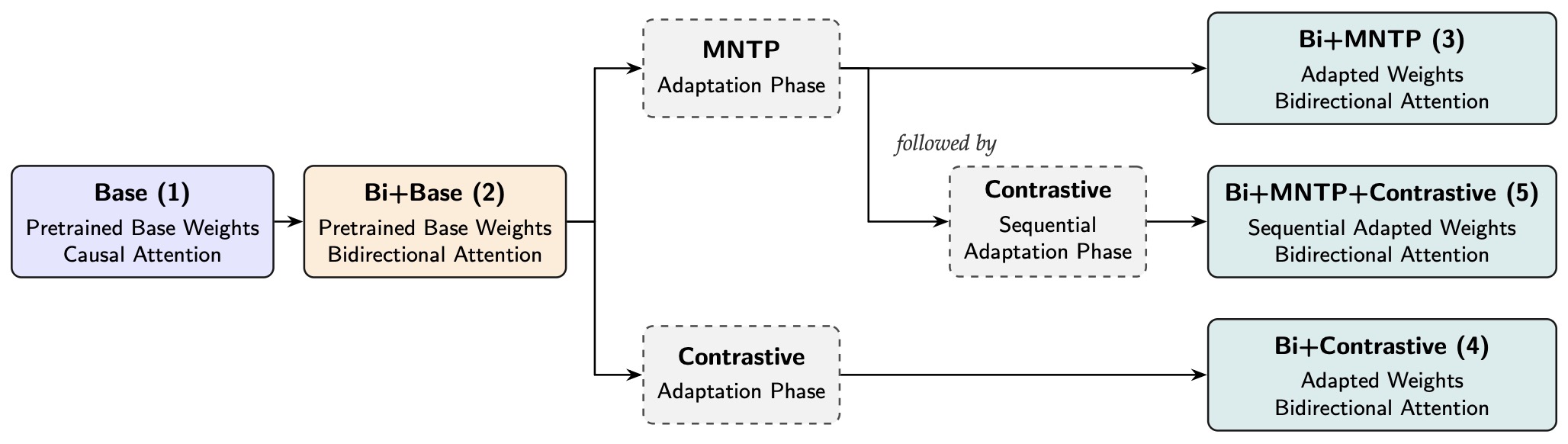
- This systematic comparison reveals that encoder adaptation is not a binary process. Different objectives contribute differently to representation quality, retrieval performance, and knowledge preservation.
Why Bidirectional Attention Alone Is Not Enough
-
One of the most important findings in BidirLM is that enabling bidirectional attention alone does not create a strong encoder.
-
After replacing the causal attention mask with a bidirectional attention pattern, the model gains access to future context, but its parameters remain optimized for causal generation.
-
Consequently, hidden states do not automatically exploit newly available context.
-
This observation mirrors findings from LLM2Vec, where simple attention-mask replacement produced weaker representations than models that underwent additional adaptation.
-
Formally, the attention modification changes token computation from:
\[h_i =f(x_{\leq i})\]-
to:
\[h_i =f(x_1,x_2,\dots,x_T)\]
-
-
However, parameter values remain unchanged. The model therefore requires additional training before full-context representations become useful for retrieval and similarity tasks.
Masked Next-Token Prediction
-
To address this mismatch, BidirLM introduces a masked next-token prediction (MNTP) adaptation phase.
-
Given an input sequence \(x=(x_1,x_2,\dots,x_T)\) and a set of masked positions \(M\), the objective is:
\[\mathcal{L}_{\text{MNTP}} =-\sum_{i \in M} \log P_\theta(x_i \mid x_{\setminus M})\] -
Unlike causal language modeling, MNTP allows both left and right context to influence predictions.
-
This adaptation phase serves several purposes:
- It teaches the model to exploit future context introduced by bidirectional attention.
- It preserves compatibility with the model’s original next-token prediction objective.
- It minimizes disruption to pretrained knowledge while adapting internal representations.
-
Importantly, MNTP is not intended to optimize retrieval performance directly. Instead, it prepares the model for later representation learning objectives.
Contrastive Adaptation for Embedding Geometry
-
Once the model can effectively use bidirectional context, BidirLM applies contrastive learning to shape the embedding space.
-
Given a query representation \(q_i\), a positive target representation \(p_i^+\), and a collection of negative representations \(p_j^-\), the contrastive objective is:
\[\mathcal{L}_{\text{contrastive}} =-\log \frac{ \exp(\mathrm{sim}(q_i,p_i^+)/\tau) }{ \exp(\mathrm{sim}(q_i,p_i^+)/\tau) +\sum_j \exp(\mathrm{sim}(q_i,p_j^-)/\tau) }\] -
This objective improves global semantic organization by aligning semantically related representations while separating unrelated examples.
-
BidirLM demonstrates that MNTP and contrastive learning play complementary roles:
- MNTP improves contextual understanding.
- Contrastive learning improves embedding geometry.
-
The strongest results are obtained when both stages are applied sequentially.
Scaling Without Original Pretraining Data
-
A practical challenge in encoder adaptation is that the original pretraining corpus is usually unavailable.
-
Large commercial and open-weight foundation models are often released without the full datasets used during training.
-
Consequently, adaptation must occur using alternative data sources while avoiding catastrophic forgetting.
-
Catastrophic forgetting refers to degradation of previously learned capabilities during fine-tuning:
- If adaptation data is too narrow, the encoder may improve on retrieval tasks while losing multilingual, coding, reasoning, or domain-specific capabilities.
Multi-Domain Adaptation Mixtures
-
To mitigate forgetting, BidirLM uses a lightweight adaptation mixture containing diverse domains.
-
The adaptation mixture includes:
- General natural language text that preserves broad semantic coverage.
- Multilingual examples that maintain cross-lingual capabilities.
- Code datasets that preserve programming knowledge.
- Mathematical content that preserves symbolic reasoning skills.
-
This design reflects a broader trend in modern embedding systems. Rather than optimizing for a single benchmark, embedding models increasingly rely on balanced mixtures that preserve generality across many downstream tasks.
Linear Weight Merging
-
BidirLM introduces linear weight merging as a mechanism for preserving pretrained knowledge.
-
Given an adapted encoder with parameters: \(\theta_{\text{adapted}}\) and the original causal model: \(\theta_{\text{base}}\), the merged model is:
-
This procedure combines encoder-specific adaptations with the broader knowledge retained in the original model.
-
The technique is closely related to Model Soups: Averaging Weights of Multiple Fine-Tuned Models by Wortsman et al. (2022), which demonstrated that averaging compatible model checkpoints can improve generalization while preserving capabilities.
-
Weight merging becomes especially important when encoder adaptation introduces narrow task specialization.
Composing Specialized Causal Models
-
Weight merging enables a second major innovation: compositionality.
-
Once a causal model has been converted into a bidirectional encoder, additional specialized causal models can be merged into the resulting representation system.
-
These specialist models may contain expertise in:
- Visual understanding learned from image-centric training.
- Audio understanding learned from speech and acoustic tasks.
- Safety alignment learned from preference optimization.
- Domain-specific knowledge learned from targeted corpora.
-
Rather than retraining a unified encoder from scratch, BidirLM transfers specialist capabilities through composition.
Building Omnimodal Encoders
-
This composition process is what transforms BidirLM from a text-encoder adaptation recipe into an omnimodal encoder framework.
-
Traditional multimodal systems often use separate towers:
- A text encoder processes language.
- A vision encoder processes images.
- An audio encoder processes sound.
-
These representations are later aligned through contrastive learning.
-
BidirLM instead proposes a fundamentally different perspective. If multiple specialist causal models share a common architecture family, their knowledge can be merged into a single bidirectional encoder.
-
The resulting encoder inherits capabilities from multiple modalities while maintaining a unified representation architecture.
Performance Analysis
-
BidirLM evaluates the effect of different adaptation strategies across retrieval and representation benchmarks.
-
The following figure (source) shows performance improvements obtained from different adaptation strategies relative to the original causal model.
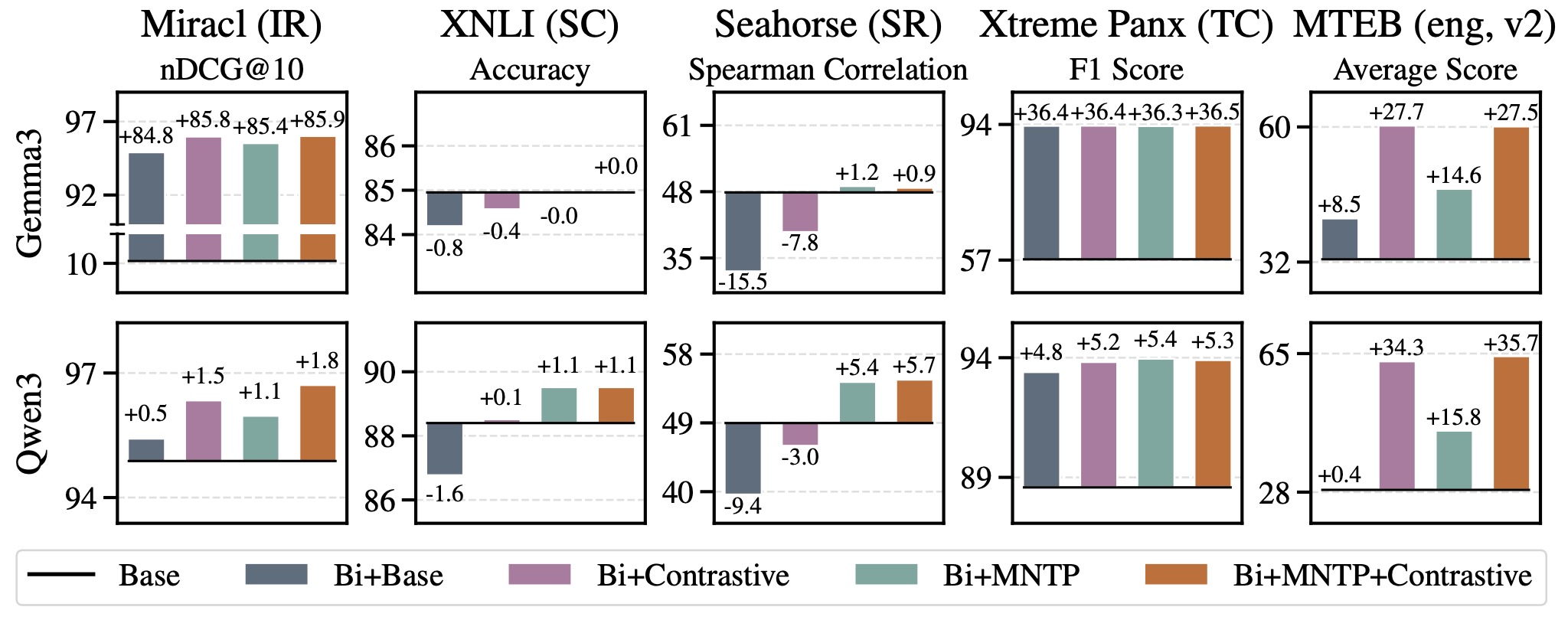
-
The results demonstrate several consistent trends:
- Bidirectional attention alone produces limited improvements.
- MNTP significantly improves representation quality.
- Contrastive learning improves retrieval-oriented geometry.
- Combining MNTP and contrastive learning produces the strongest overall performance.
- Weight merging helps preserve broader capabilities during adaptation.
-
These findings support the broader conclusion that successful encoder adaptation requires both architectural modification and objective-level adaptation.
Implications for Future Encoder Architectures
-
BidirLM suggests that future embedding systems may increasingly be constructed through adaptation and composition rather than through standalone encoder pretraining.
-
This perspective offers several advantages:
- Existing foundation models can be reused rather than discarded.
- Specialized models can contribute capabilities without requiring unified retraining.
- Embedding systems can evolve alongside generative foundation models.
- New modalities can potentially be incorporated through composition rather than redesign.
-
More broadly, BidirLM demonstrates that the distinction between generative models and embedding models is becoming increasingly blurred. A sufficiently capable generative model can often be transformed into a high-quality encoder, and multiple such encoders can subsequently be composed into a unified representation system.
From Text to Omnimodal Embeddings
Limitations of Text Embeddings
-
Modern embedding systems are no longer confined to text. The same geometric principle that makes text embeddings useful for semantic search also extends to images, audio, video, structured documents, and interleaved multimodal inputs. A text embedding model maps language into a vector space where semantically related passages are nearby, but real-world information rarely appears as text alone. Product catalogs combine images, metadata, descriptions, and reviews; enterprise documents combine prose, tables, charts, screenshots, and layout; videos combine visual frames, speech, captions, music, and temporal events; and scientific materials often combine equations, diagrams, figures, and explanatory text.
-
This creates a structural limitation for text-only encoders. A text encoder can represent captions, transcripts, or OCR-extracted text, but it cannot directly represent visual layout, acoustic tone, image composition, temporal motion, or modality interactions unless those signals are first converted into text. Such conversions can be useful, but they are lossy. For example, automatic speech recognition may preserve words while losing prosody, hesitation, speaker emphasis, and nonverbal audio cues. OCR may recover visible text while losing layout, scale, visual grouping, and diagrammatic relationships. Image captioning may summarize a picture while omitting fine-grained visual evidence required for retrieval.
-
A multimodal embedding model generalizes the familiar text embedding function:
\[f_\theta : \mathcal{X}_{\text{text}} \rightarrow \mathbb{R}^d\]-
into a broader function over heterogeneous inputs:
\[f_\theta : \mathcal{X}_{\text{multi}} \rightarrow \mathbb{R}^d\]where:
\[\mathcal{X}_{\text{multi}} =\mathcal{X}_{\text{text}} \cup \mathcal{X}_{\text{image}} \cup \mathcal{X}_{\text{audio}} \cup \mathcal{X}_{\text{video}} \cup \mathcal{X}_{\text{document}} \cup \mathcal{X}_{\text{interleaved}}\]
-
-
The goal is not merely to support more input formats. The goal is to learn a representation space in which semantically related inputs are close even when they come from different modalities:
\[\mathrm{sim} \left( f_\theta(x^{(\text{text})}), f_\theta(y^{(\text{image})}) \right) \gg \mathrm{sim} \left( f_\theta(x^{(\text{text})}), f_\theta(z^{(\text{image})}) \right)\]- where \(x^{(\text{text})}\) and \(y^{(\text{image})}\) describe the same concept, while \(z^{(\text{image})}\) is unrelated.
-
This is the conceptual bridge from text encoders to omnimodal embedding systems. In a text-only system, semantic similarity is computed within language. In an omnimodal system, semantic similarity becomes a cross-modal operation: a text query can retrieve an image, an image can retrieve a document, a video clip can retrieve a caption, and an audio recording can retrieve related visual or textual evidence.
Representation Transfer
-
Before native multimodal embedding models became practical, an important intermediate step was the use of LLMs to improve embedding models through representation transfer. Gecko: Versatile Text Embeddings Distilled from Large Language Models by Lee et al. (2024) introduced a two-stage LLM-powered distillation pipeline in which an LLM first generates synthetic task-query pairs from passages and then relabels positive and hard-negative passages after retrieval. This is important because it shows that an LLM can transfer broad semantic knowledge into a compact retriever without becoming the retriever itself.
-
The following figure (source) shows the Gecko training pipeline, where an LLM generates task-query pairs and mines positive and negative passages to create FRet, a retrieval-focused training dataset.
-
Gecko illustrates the data-centric route from LLMs to embeddings. The embedding model remains a compact retriever, while the LLM supplies higher-quality supervision. This design is especially useful when retrieval training data is incomplete, noisy, or expensive to annotate. Instead of relying only on human-labeled query-document pairs, the training set can be expanded using generated queries, task instructions, LLM-selected positives, and hard negatives.
-
This transfer idea also clarifies the relationship between LLM-derived text embeddings and multimodal embeddings. LLM-derived embedding models demonstrate that foundation-model knowledge can be compressed, adapted, or projected into reusable vector spaces. Native multimodal embedding models extend the same principle across modalities: rather than transferring only linguistic knowledge into a text embedding model, they transfer multimodal understanding into a unified representation space.
Unified Functions
-
Earlier multimodal retrieval systems typically relied on separate modality-specific encoders. A text encoder processed text, a vision encoder processed images, and an audio encoder processed sound. These encoders were then aligned through a shared embedding objective. This modular design made engineering sense because each modality had different raw input structure, tokenization, preprocessing, and architecture requirements.
-
A typical image-text dual-encoder system can be written as:
-
The model then learns to place matched image-text pairs close together. Learning Transferable Visual Models From Natural Language Supervision by Radford et al. (2021) introduced CLIP as a large-scale contrastive image-text model trained to predict which caption belongs with which image, establishing a practical foundation for zero-shot image classification and text-image retrieval. Scaling Up Visual and Vision-Language Representation Learning With Noisy Text Supervision by Jia et al. (2021) introduced ALIGN, showing that noisy web-scale image-alt-text pairs can train strong cross-modal representations using a simple dual-encoder architecture.
-
The standard contrastive objective for paired image-text training can be written as:
\[\mathcal{L}_{\text{contrastive}} =-\log \frac{ \exp \left( \mathrm{sim} \left( f_{\theta_I}(x_i), f_{\theta_T}(t_i) \right) /\tau \right) }{ \sum_{j=1}^{B} \exp \left( \mathrm{sim} \left( f_{\theta_I}(x_i), f_{\theta_T}(t_j) \right) /\tau \right) }\]- where \(x_i\) is an image, \(t_i\) is its paired text description, \(B\) is the batch size, and \(\tau\) is a temperature parameter.
-
CLIP-style and ALIGN-style systems were major advances because they made cross-modal retrieval practical at scale. However, they still preserve a modular separation between modality encoders. Each modality is processed independently, and alignment occurs at the embedding level. This can limit deep modality fusion, especially when an input itself contains interleaved modalities that must be interpreted jointly.
-
Native multimodal embedding systems address this limitation by making multimodality part of the embedding model rather than an external alignment layer. Gemini Embedding 2: A Native Multimodal Embedding Model from Gemini by Shanbhogue et al. (2026) builds on Gemini’s multimodal foundation capabilities to embed text, images, audio, video, documents, and arbitrary interleavings of these inputs into a unified representation space. This changes the architecture from separate mappings plus alignment into a unified embedding function:
- This unified view is the main conceptual difference between late-fusion multimodal architectures and native omnimodal embeddings. Late-fusion systems align separate representations after modality-specific encoding. Native omnimodal systems aim to encode heterogeneous inputs directly into a shared semantic geometry, allowing modality interactions to influence the resulting representation earlier and more deeply.
Retrieval Impact
- The shift from modality-specific encoders to unified embedding functions changes the structure of retrieval systems. In a modular system, each modality often requires its own index, preprocessing logic, and retrieval pathway. In a unified system, heterogeneous objects can be embedded into the same vector store:
- A query from any supported modality can then retrieve the nearest items by similarity:
-
This enables retrieval systems where a text query retrieves a video segment, an image retrieves a relevant document, an audio clip retrieves related text, or a mixed image-and-text query retrieves a visually rich file. The practical result is a more general retrieval substrate for multimodal search, multimodal RAG, recommendation, clustering, and enterprise knowledge discovery.
-
The transition from text encoders to unified omnimodal embeddings therefore reflects both a modeling shift and a systems shift. At the modeling level, the embedding function expands from language-only representations to heterogeneous multimodal representations. At the systems level, retrieval infrastructure moves from modality-specific stacks toward shared vector spaces that can index and compare many forms of data through the same geometric interface.
Gemini Embedding 2
-
Gemini Embedding 2 represents the native multimodal branch of the transition from text encoders to unified omnimodal embeddings. Earlier systems often aligned modality-specific encoders after separate processing, while Gemini Embedding 2 starts from a multimodal foundation model and trains an embedding system directly on top of that multimodal backbone. Gemini Embedding 2: A Native Multimodal Embedding Model from Gemini by Shanbhogue et al. (2026) introduces this model as a unified embedding system for text, images, audio, video, documents, and arbitrary combinations of these inputs.
-
This distinction matters because native multimodal embeddings avoid treating images, audio, video, and documents as secondary artifacts that must first be converted into text. Instead, the model can embed raw or structured multimodal inputs directly, allowing visual, acoustic, temporal, document-layout, and linguistic signals to contribute to the final representation. Gemini Embedding 2: Our first natively multimodal embedding model describes the system as mapping text, images, video, audio, and documents into one embedding space for multimodal retrieval, classification, semantic search, clustering, and RAG.
Native Backbone
-
Gemini Embedding 2 builds on the broader Gemini model family, whose foundation architecture is designed for multimodal processing rather than text-only generation. Gemini: A Family of Highly Capable Multimodal Models by Team Gemini et al. (2023) introduced Gemini as a family of multimodal models capable of processing text, images, audio, and video, which makes it a natural backbone for a native multimodal embedding system.
-
At a high level, Gemini Embedding 2 can be described as:
\[x_{\text{multi}} \rightarrow \text{Gemini Backbone} \rightarrow H \rightarrow \text{Pooling} \rightarrow \text{Projection} \rightarrow \mathbf{z}\]- where \(x_{\text{multi}}\) may contain one modality or several interleaved modalities, \(H\) denotes contextual hidden states from the multimodal backbone, and \(\mathbf{z} \in \mathbb{R}^{d}\) is the final embedding vector.
-
A native multimodal backbone changes the representation problem. In a dual-encoder system, separate encoders must later agree in vector space. In Gemini Embedding 2, the backbone can model cross-modal interactions before the final embedding projection. This is especially important for inputs where meaning arises from the interaction between modalities, such as a screenshot plus a text instruction, a video clip plus a query about a temporal event, or a PDF page containing figures, captions, tables, and surrounding prose.
-
The following figure (source) shows the conceptual Gemini Embedding 2 workflow, where text, image, video, audio, documents, and combinations of these inputs are mapped into a single high-dimensional vector space.
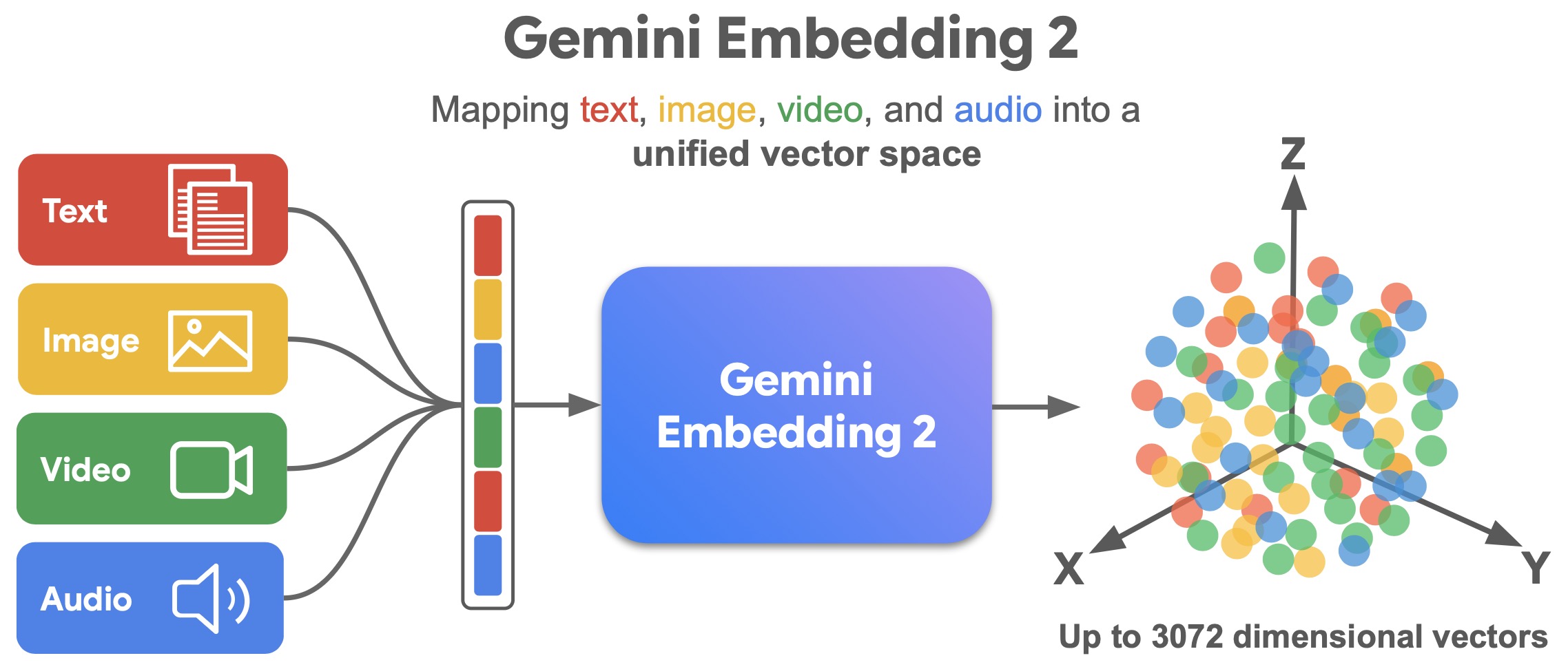
Input Coverage
-
Gemini Embedding 2 directly supports text, image, video, audio, document, and interleaved multimodal inputs within a shared embedding interface. Gemini Embedding 2: Our first natively multimodal embedding model states that the model supports text inputs with up to 8192 input tokens, image inputs with up to 6 images per request in PNG or JPEG formats, video inputs up to 120 seconds in MP4 or MOV formats, and native audio inputs without requiring intermediate transcription.
-
This broad input coverage is important for implementation because it reduces the need to build separate modality-specific preprocessing and embedding paths. A retrieval system can expose a unified embedding API that accepts different input types, produces a vector, and stores that vector in a common index. Modality-specific preprocessing may still be needed for file normalization, segmentation, metadata extraction, or batching, but the semantic representation step is unified.
-
Formally, the input can be represented as an ordered multimodal sequence:
\[x=\left[ x_1^{(m_1)}, x_2^{(m_2)}, \dots, x_T^{(m_T)} \right]\]- where each element \(x_i^{(m_i)}\) belongs to a modality \(m_i \in {\text{text}, \text{image}, \text{audio}, \text{video}, \text{document}}\). The embedding model maps the entire sequence into one representation:
- This formulation is more general than embedding each modality separately and averaging or concatenating the resulting vectors. It allows the model to treat multimodal inputs as structured semantic objects rather than independent media fragments.
Training Objective
-
Gemini Embedding 2 is trained through multi-task, multi-stage contrastive learning over diverse multimodal tasks. Gemini Embedding 2: A Native Multimodal Embedding Model from Gemini by Shanbhogue et al. (2026) describes the training process as leveraging Gemini’s multimodal capabilities and using a curated set of tasks to generalize across document retrieval, video recommendation, audio-based search, RAG applications, and interleaved multimodal retrieval.
-
A generalized multimodal contrastive objective can be written as:
\[\mathcal{L}_{\text{multi}} =-\log \frac{ \exp \left( \mathrm{sim} \left( f_\theta(x_i^{(m)}), f_\theta(x_i^{(n)}) \right) /\tau \right) }{ \sum_{j=1}^{B} \exp \left( \mathrm{sim} \left( f_\theta(x_i^{(m)}), f_\theta(x_j) \right) /\tau \right) }\]- where \(m\) and \(n\) may denote the same or different modalities, \(B\) is the number of candidates in the batch, \(\tau\) is a temperature parameter, and \(\mathrm{sim}(\cdot,\cdot)\) is typically cosine similarity.
-
The multi-stage aspect is important. Early stages can help adapt the multimodal backbone to produce retrieval-ready representations, while later stages can specialize the embedding geometry for retrieval, classification, and cross-modal matching. This differs from a narrow CLIP-style objective over image-text pairs because the training distribution spans many modality pairs and task types rather than a single alignment pathway.
Output Dimensions
-
Gemini Embedding 2 supports high-dimensional embeddings while also offering flexible output dimensionality. The maximum embedding dimensionality is 3072, and smaller output dimensions can be used when storage, latency, or index size matters. This flexibility is essential in production retrieval systems because embedding dimension directly affects vector index memory, retrieval throughput, network transfer cost, and cache footprint.
-
If a corpus contains \(N\) items and embeddings have dimensionality \(d\) with \(b\) bytes per component, the raw vector storage cost is approximately:
-
For example, reducing the dimensionality from \(3072\) to \(768\) yields an approximate \(4\times\) reduction in raw vector storage, before accounting for index overhead or quantization.
-
This dimensional flexibility is closely related to Matryoshka Representation Learning by Kusupati et al. (2022), which trains embeddings so that shorter prefixes remain useful representations. Under this approach, an embedding:
\[\mathbf{z} =(z_1,z_2,\dots,z_d)\]-
can be truncated to:
\[\mathbf{z}_{1:k} =(z_1,z_2,\dots,z_k)\]- while preserving much of the semantic structure needed for retrieval. In practice, this allows the same model family to serve high-recall cloud retrieval systems and lower-latency or storage-constrained retrieval systems.
-
Native Audio
-
Native audio retrieval is one of the clearest examples of why native multimodal embeddings can outperform conversion-based pipelines. A traditional pipeline often performs automatic speech recognition first, converts audio into text, and then embeds the transcript. That cascade can lose prosody, speaker emphasis, hesitations, background sounds, and acoustic cues that may be relevant to retrieval.
-
Gemini Embedding 2 directly embeds raw audio. Gemini Embedding 2: A Native Multimodal Embedding Model from Gemini by Shanbhogue et al. (2026) evaluates native audio retrieval on the Massive Sound Embedding Benchmark and reports that direct audio processing achieves a higher average retrieval \(\mathrm{mrr}@10\) than an ASR-based cascade, showing that native audio embeddings can preserve useful information lost during transcription.
-
This result is not only a benchmark improvement. It highlights a system-design principle: native multimodal retrieval avoids unnecessary lossy intermediate representations. When the source modality contains information not fully expressible in text, embedding the source directly can improve retrieval fidelity.
Results
-
The empirical significance of Gemini Embedding 2 is not only that it supports more modalities, but that multimodal capability does not appear to weaken text performance. Gemini Embedding 2: A Native Multimodal Embedding Model from Gemini by Shanbhogue et al. (2026) reports strong results across multimodal retrieval, multilingual text retrieval, and code retrieval, including evaluations on MSCOCO, Flickr30k, MSR-VTT, MMTEB, MTEB Code, CoIR, and MSEB.
-
The following figure (source) shows Gemini Embedding 2 performance across multimodal retrieval tasks spanning image, text, video, and document modalities.
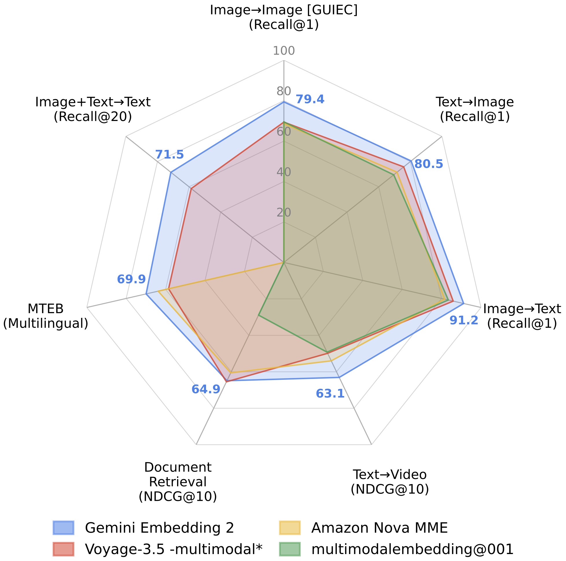
- The results support a broader conclusion: native multimodal embeddings can serve as general-purpose representation infrastructure rather than task-specific retrieval components. A single embedding model can support text retrieval, image-text retrieval, video search, audio retrieval, document retrieval, and mixed-modality retrieval without requiring each use case to maintain a completely separate encoder stack.
Design Position
-
Gemini Embedding 2 occupies a distinct position in the modern embedding design space. Gecko demonstrates how LLM knowledge can be distilled into compact retrievers through synthetic task-query generation and LLM-based relabeling. LLM2Vec and BidirLM demonstrate how decoder LLMs can be adapted into bidirectional encoders through attention changes, masking objectives, contrastive learning, and weight merging. Gemini Embedding 2 instead shows the native multimodal route: begin with a multimodal foundation model, train embeddings directly on top of that backbone, and produce a unified representation space spanning text, images, audio, video, documents, and interleaved inputs.
-
This positioning makes Gemini Embedding 2 a natural bridge between LLM-derived text embeddings and full omnimodal embedding systems. It preserves the central idea that embeddings are specialized projections of foundation-model understanding, while expanding the representation domain from text to heterogeneous multimodal inputs.
Unified Encoders
-
The transition from text encoders to omnimodal embeddings is also a transition from modular systems to unified encoders. In earlier multimodal systems, each modality was handled by a dedicated model: a language encoder represented text, a vision encoder represented images, an audio encoder represented sound, and additional alignment mechanisms connected the resulting spaces. This design made sense when modalities were treated as fundamentally separate data types, but it becomes increasingly inefficient when applications require joint reasoning over mixed media.
-
Modern embedding systems move toward unified encoders that share parameters across modalities, learn joint semantic representations, and support flexible downstream tasks. This does not mean that every modality is processed identically at the lowest level, since images, video, audio, text, and documents still require different tokenization or preprocessing steps. Rather, it means that the representation layer exposed to retrieval and downstream systems becomes unified: every supported input can be mapped into the same vector space and compared using the same similarity function.
-
A unified encoder can be expressed as:
\[\mathbf{z} =f_\theta(x^{(m)})\]- where \(m\) denotes the input modality, and \(\mathbf{z} \in \mathbb{R}^{d}\) lies in the same embedding space regardless of whether \(x^{(m)}\) is text, image, audio, video, document content, or an interleaved multimodal input.
Design Space
- The modern embedding design space can be understood as several complementary approaches to unification. Text-only embedding systems focus on language and optimize for retrieval, clustering, and semantic similarity within textual corpora.
- LLM-derived systems such as Gecko: Versatile Text Embeddings Distilled from Large Language Models by Lee et al. (2024), LLM2Vec: Large Language Models Are Secretly Powerful Text Encoders by BehnamGhader et al. (2024), and BidirLM: From Text to Omnimodal Bidirectional Encoders by Adapting and Composing Causal LLMs by Boizard et al. (2026) reuse generative model knowledge through distillation, decoder-to-encoder conversion, and bidirectional adaptation.
- Native multimodal systems such as Gemini Embedding 2: A Native Multimodal Embedding Model from Gemini by Shanbhogue et al. (2026) instead train a unified embedding model on top of a multimodal foundation backbone.
| Paradigm | Architecture | Primary Limitation |
|---|---|---|
| Text embeddings | Encoder-only text representation model trained for semantic similarity and retrieval | Text-only scope limits direct retrieval over images, audio, video, and visually rich documents |
| EmbeddingGemma-style lightweight LLM-derived embeddings | Compact encoder initialized from Gemma-derived representations and optimized for efficient text embedding deployment | Text-focused design prioritizes efficiency and general-purpose retrieval rather than native multimodal representation |
| Gecko-style distillation | Compact retriever trained from LLM-generated task-query pairs, relabeled positives, and hard negatives | Knowledge transfer is indirect because the LLM supplies supervision but does not become the deployed embedding model |
| CLIP-style alignment | Dual-encoder architecture that separately processes images and text before aligning matched pairs in a shared space | Modality fusion is limited because deep interactions across modalities occur only after separate representation extraction |
| BidirLM-style adaptation | Causal LLM converted into a bidirectional encoder through attention adaptation, masked next-token prediction, contrastive learning, and weight merging | Successful conversion requires careful adaptation to avoid catastrophic forgetting and to teach the model to exploit bidirectional context |
| Gemini Embedding 2-style native multimodal embeddings | Unified multimodal embedding model trained on top of a multimodal Gemini foundation backbone | The approach depends on access to a strong native multimodal foundation model and carefully balanced multimodal training mixtures |
- This design space shows that there is no single path to unified embeddings. Some systems transfer knowledge through data, some through architectural adaptation, and some through native multimodal training. The common goal is to expose foundation-model understanding as reusable vectors that can be indexed, compared, and retrieved efficiently.
System Simplification
- Unified encoders reduce system complexity by replacing modality-specific retrieval paths with a common representation interface. In a modular system, developers may need one pipeline for text retrieval, another for image retrieval, another for audio search, another for video indexing, and additional logic to align or rerank results across modalities. In a unified embedding system, the pipeline becomes structurally simpler:
-
This simplicity has practical consequences. The same retrieval infrastructure can support semantic search, multimodal search, document retrieval, recommendation, clustering, deduplication, and retrieval-augmented generation. A unified index can store vectors from different modalities, while metadata can preserve modality, source, timestamp, access control, and segmentation information.
-
A corpus containing heterogeneous assets can be represented as:
\[\mathcal{C} ={ (e_i, m_i, \mu_i) }_{i=1}^{N}\]- where \(e_i\) is the embedding, \(m_i\) is the modality label, and \(\mu_i\) contains metadata such as source, chunk boundary, document page, timestamp, frame range, language, or permissions.
-
At query time, retrieval can combine vector similarity with metadata filtering:
\[x^\star =\arg\max_{x_i \in \mathcal{C}, ; \mu_i \in \mathcal{F}} \mathrm{sim} \left( f_\theta(q), e_i \right)\]- where \(\mathcal{F}\) denotes application-specific filters such as allowed document collections, modality constraints, time ranges, or access-control rules.
Implementation Notes
-
Building unified embedding systems requires several implementation decisions that are less visible in model papers but important in production.
-
First, inputs must be segmented at the right granularity. Text may be chunked by paragraphs or semantic sections, video may be segmented by time windows or scene boundaries, audio may be segmented by utterances or fixed windows, and documents may be embedded at page, section, table, or figure level. Poor segmentation can reduce retrieval quality even when the embedding model is strong.
-
Second, modality metadata should be preserved alongside embeddings. Unified vector spaces make retrieval modality-agnostic, but downstream systems often still need modality-aware handling. A retrieved video segment may require timestamp playback, an image may require rendering, an audio clip may require playback or transcription, and a document chunk may require page-level citation.
-
Third, ranking often benefits from a two-stage design. A unified embedding model can perform first-stage retrieval efficiently, while a reranker or generative model can perform second-stage reasoning over retrieved candidates. This mirrors the broader retrieval architecture where dense embeddings provide high-recall candidate retrieval and cross-encoders or multimodal models provide high-precision reranking.
-
Fourth, unified embedding systems should support dimensionality and storage trade-offs. High-dimensional embeddings can improve recall but increase index size and latency. Techniques such as Matryoshka Representation Learning by Kusupati et al. (2022) allow shorter prefixes of embeddings to remain useful, making it possible to deploy different dimensions for different retrieval settings without retraining separate models.
Retrieval Implications
-
The move to unified encoders changes retrieval from a modality-specific operation into a semantic operation over heterogeneous data. The relevant question becomes less “which image is visually similar to this image?” or “which document contains these words?” and more “which item, regardless of modality, best matches the user’s information need?”
-
This shift is particularly important for retrieval-augmented generation. Traditional RAG systems retrieve text passages and pass them to a language model. Omnimodal RAG systems can retrieve images, charts, video segments, tables, audio clips, and documents, then provide richer evidence to downstream reasoning models. Retrieval-Augmented Generation for Knowledge-Intensive NLP Tasks by Lewis et al. (2020) introduced RAG as a framework combining parametric generation with non-parametric retrieval, and native multimodal embeddings extend the retrieval side of that framework beyond text.
-
Unified encoders also improve enterprise and scientific search. A query about an experiment may retrieve a figure from a paper, a table from a PDF, a lab-note paragraph, and a video demonstration. A query about a customer issue may retrieve a support article, a screenshot, a meeting transcript, and a product video. This breadth is difficult to support cleanly with modality-specific indexes.
-
The broader implication is that embeddings become an infrastructure layer rather than a model-specific feature. Once heterogeneous data is embedded into a shared space, the same representations can support search, clustering, recommendation, deduplication, monitoring, analytics, and agent memory.
Training Omnimodal Embeddings
- Training omnimodal embedding systems requires broader data mixtures and more complex objective design than training text-only encoders. A text retrieval model can be trained on query-document pairs, semantic similarity labels, or instruction-response examples.
- A native multimodal embedding model must additionally align language with images, audio, video, document layout, charts, tables, and interleaved inputs while preserving strong performance on text-only retrieval. Gemini Embedding 2: A Native Multimodal Embedding Model from Gemini by Shanbhogue et al. (2026) frames this as a multi-task, multi-stage contrastive training problem over heterogeneous data.
- The central training lesson is that omnimodal embeddings are not produced by simply adding more modalities to a text encoder. They require balanced multimodal data mixtures, contrastive objectives that operate across modalities, careful hard-negative construction, staged training, checkpoint merging, and dimensionality-aware optimization. These design choices allow the embedding space to preserve text quality while adding image, audio, video, document, and interleaved-input retrieval capabilities.
Data Mixtures
-
Omnimodal training depends on diverse paired and grouped examples. A training mixture may include text-text pairs for semantic retrieval, image-text pairs for visual grounding, audio-text pairs for speech and sound retrieval, video-text pairs for temporal visual understanding, document-query pairs for visually rich retrieval, and interleaved examples where meaning depends on multiple modalities at once.
-
This can be represented as:
\[\mathcal{D}=\left\{(x_i^{(m)}, x_i^{(n)}, y_i)\right\}_{i=1}^{N}\]- where \(m\) and \(n\) denote modalities, and \(y_i\) indicates whether the pair is semantically matched. In practice, the dataset is not a single homogeneous table. It is a mixture of tasks, modalities, domains, and supervision types. The mixture design matters because overrepresenting one modality can improve that modality while weakening others.
-
For implementation, data pipelines typically need modality-specific preprocessing before unified embedding training. Text must be tokenized, images must be resized or patchified, audio must be segmented or converted into acoustic tokens, video must be sampled across time, and documents may require page segmentation, OCR, layout extraction, or multimodal tokenization. The important architectural point is that these preprocessing steps feed a unified representation model rather than separate retrieval systems.
Contrastive Alignment
-
Contrastive learning remains the central objective for organizing shared embedding spaces. The model is trained so that semantically matched items have high similarity and mismatched items have low similarity. For multimodal examples, the positive pair may come from the same modality or different modalities.
-
A generalized multimodal contrastive loss is:
\[\mathcal{L}_{\text{contrastive}} =-\log \frac{ \exp \left( \mathrm{sim} \left( f_\theta(x_i^{(m)}), f_\theta(x_i^{(n)}) \right) /\tau \right) }{ \sum_{j=1}^{B} \exp \left( \mathrm{sim} \left( f_\theta(x_i^{(m)}), f_\theta(x_j) \right) /\tau \right) }\]- where \(x_i^{(m)}\) is an anchor from modality \(m\), \(x_i^{(n)}\) is a matched item from modality \(n\), \(B\) is the candidate set size, and \(\tau\) is a temperature parameter.
-
Learning Transferable Visual Models From Natural Language Supervision by Radford et al. (2021) established this approach for image-text alignment with CLIP, while Scaling Up Visual and Vision-Language Representation Learning With Noisy Text Supervision by Jia et al. (2021) showed that noisy web-scale image-text data could train strong dual-encoder representations through ALIGN. Native omnimodal systems generalize this contrastive principle beyond image-text pairs to many modality combinations.
Multi-Stage Training
-
Omnimodal models often use staged training rather than a single training run over one uniform dataset. Early stages can adapt a foundation model to produce retrieval-ready embeddings. Later stages can specialize the model toward difficult retrieval, multilingual retrieval, document understanding, code retrieval, audio retrieval, or video retrieval. This staged design helps avoid the instability that can arise when very heterogeneous objectives are mixed too early or too aggressively.
-
A generic multi-stage recipe can be written as:
\[\theta_0 \rightarrow \theta_1 \rightarrow \theta_2 \rightarrow \theta_3\]- where \(\theta_0\) is the foundation model, \(\theta_1\) is adapted on broad multimodal contrastive data, \(\theta_2\) is refined on task-specific retrieval mixtures, and \(\theta_3\) is selected or merged for deployment.
-
Gemini Embedding 2 uses this type of multi-stage training to balance broad multimodal coverage with retrieval quality. Gemini Embedding 2: A Native Multimodal Embedding Model from Gemini by Shanbhogue et al. (2026) reports that the model is trained through staged contrastive learning and model souping to improve performance across diverse retrieval tasks without collapsing into a narrow modality-specific system.
Hard Negatives
-
Hard negatives are especially important in multimodal training because many incorrect candidates can be superficially similar. An image of a red car and an image of a red truck may be visually close but semantically different for a fine-grained query. A transcript about a medical scan and a figure from a medical paper may share terminology but answer different retrieval needs. A video segment and a caption may share objects but differ in action or temporal structure.
-
Given an anchor \(x_i\), a positive \(x_i^+\), and hard negatives \({x_{i,1}^-, \dots, x_{i,K}^-}\), the loss can be written as:
- Gecko demonstrates the importance of high-quality negative construction in text retrieval. Gecko: Versatile Text Embeddings Distilled from Large Language Models by Lee et al. (2024) uses an LLM to relabel positives and hard negatives after retrieval, showing that better supervision can substantially improve compact embedding models. The same principle generalizes to multimodal systems, where hard negatives must often be mined within and across modalities.
Model Souping
-
When a model is trained across many modalities and tasks, one checkpoint may perform best on text retrieval, another on image retrieval, another on video retrieval, and another on document retrieval. Selecting a single checkpoint can therefore create trade-offs. Model souping addresses this by averaging compatible checkpoints.
-
Given checkpoints \(\theta_1,\theta_2,\dots,\theta_K\), a merged model can be written as:
\[\theta_{\text{soup}} =\sum_{k=1}^{K} \alpha_k \theta_k\]- where:
-
Model Soups: Averaging Weights of Multiple Fine-Tuned Models Improves Accuracy Without Increasing Inference Time by Wortsman et al. (2022) introduced model souping as a way to improve generalization by averaging fine-tuned checkpoints. Gemini Embedding 2 applies this idea in the multimodal embedding setting to combine strengths from different training stages and task mixtures. BidirLM uses a related but distinct form of weight merging to preserve pretrained knowledge while adapting causal models into bidirectional encoders, as described in BidirLM: From Text to Omnimodal Bidirectional Encoders by Adapting and Composing Causal LLMs by Boizard et al. (2026).
Dimensional Training
-
Omnimodal models must also be trained with deployment constraints in mind. A high-dimensional embedding may improve retrieval quality, but it increases storage cost and retrieval latency. Matryoshka-style training addresses this by making shorter vector prefixes useful.
-
If the full embedding is:
\[\mathbf{z} =(z_1,z_2,\dots,z_d)\]-
then a truncated embedding is:
\[\mathbf{z}_{1:k} =(z_1,z_2,\dots,z_k)\]- where \(k < d\).
-
-
A nested training objective can be written as:
- Matryoshka Representation Learning by Kusupati et al. (2022) introduced this approach to make embeddings useful at multiple dimensionalities. Gemini Embedding 2 uses dimensional flexibility to support different retrieval deployments, while EmbeddingGemma applies related ideas for efficient text embedding under storage and latency constraints.
System Implications
- Unified omnimodal embeddings change system design by replacing modality-specific retrieval stacks with a shared representation layer. Earlier systems often maintained separate indexes for documents, images, videos, audio clips, and structured files. Native multimodal embeddings allow these assets to be embedded into a common vector space, making retrieval, clustering, ranking, recommendation, and RAG operate through a unified interface.
- The practical impact of omnimodal embeddings is that retrieval infrastructure becomes simpler, broader, and more reusable. Instead of building separate retrieval systems for every modality, applications can embed heterogeneous content into a shared vector space, preserve modality-specific metadata, retrieve candidates through a common index, and use reranking or generation for task-specific reasoning. This architecture supports multimodal search, multimodal RAG, recommendation, analytics, and agentic workflows through the same underlying representation layer.
Unified Indexes
-
A unified index stores embeddings from many modalities in the same retrieval system:
\[\mathcal{C} ={ (e_i, m_i, \mu_i) }_{i=1}^{N}\]- where \(e_i\) is the embedding, \(m_i\) denotes the modality, and \(\mu_i\) stores metadata such as source, timestamp, page number, document section, frame range, language, access-control policy, or chunk boundary.
-
A query from any supported modality can retrieve nearest neighbors from the same index:
- This enables retrieval flows where a text query retrieves a video segment, an image retrieves a document, an audio clip retrieves related text, and a mixed-modality query retrieves a visually rich report. Gemini Embedding 2: A Native Multimodal Embedding Model from Gemini by Shanbhogue et al. (2026) demonstrates this unified retrieval principle across text, images, video, audio, and documents.
Multimodal RAG
-
Retrieval-Augmented Generation originally focused on text retrieval, where a query retrieves passages that are then supplied to a generator. Retrieval-Augmented Generation for Knowledge-Intensive NLP Tasks by Lewis et al. (2020) introduced this architecture as a way to combine parametric generation with non-parametric retrieval.
-
Omnimodal embeddings extend this pattern by allowing the retrieval corpus to contain heterogeneous evidence:
- The resulting pipeline becomes:
- This is especially useful when answers depend on evidence that is not fully captured by text alone. A medical query may retrieve a diagnostic image and a report, a troubleshooting query may retrieve screenshots and documentation, and an educational query may retrieve diagrams, lecture clips, and transcript segments. Gemini Embedding 2: Our first natively multimodal embedding model describes this capability as a foundation for multimodal retrieval and RAG over text, images, video, audio, and documents.
Metadata and Filtering
-
Unified vector spaces do not eliminate the need for structured metadata. In practice, metadata becomes more important because heterogeneous results require modality-aware handling. A retrieved PDF page must preserve page number and source file, a video segment must preserve timestamp and duration, an audio segment must preserve speaker or time range when available, and an image must preserve provenance, resolution, and permissions.
-
Retrieval can combine vector similarity with metadata constraints:
\[x^\star =\arg\max_{x_i \in \mathcal{C}, ; \mu_i \in \mathcal{F}} \mathrm{sim} \left( f_\theta(q), e_i \right)\]- where \(\mathcal{F}\) denotes filters such as permitted collections, allowed modalities, recency windows, language, document type, or access-control rules.
-
This hybrid design is important for production systems. Vector similarity retrieves semantically relevant items, while metadata ensures that the results satisfy application constraints, compliance requirements, and user permissions.
Chunking and Segmentation
-
Omnimodal retrieval quality depends heavily on how assets are segmented before embedding. Text may be chunked by semantic sections, paragraphs, or sliding windows. Documents may be embedded by page, section, figure, table, or layout region. Audio may be segmented by utterance, speaker turn, or time window. Video may be segmented by scenes, frames, shots, transcript windows, or detected events.
-
Poor segmentation can degrade retrieval even when the embedding model is strong. If chunks are too large, embeddings may blur multiple unrelated concepts. If chunks are too small, embeddings may lose context. For a document or video asset \(A\), segmentation can be represented as:
\[A={s_1,s_2,\dots,s_K}\]-
with embeddings:
\[e_k =f_\theta(s_k)\]
-
-
The retrieval system then returns the most relevant segments rather than the entire asset. This improves precision and allows downstream generators to cite or display the exact passage, page, frame range, or audio span that supports an answer.
Reranking
- Unified embeddings are often most effective as a first-stage retriever. A first-stage vector search retrieves a candidate set:
- A second-stage reranker can then perform more expensive cross-attention or multimodal reasoning over the candidates:
- This two-stage architecture balances recall and precision. Embeddings provide scalable retrieval over large corpora, while rerankers improve ordering among the top candidates. In multimodal systems, reranking is especially useful because the first-stage embedding may retrieve semantically broad candidates, while the second stage can inspect fine-grained visual, textual, temporal, or acoustic evidence.
Reuse
- A major systems advantage of embeddings is reuse. Once an asset is embedded, the same vector can support multiple tasks:
-
The same representation can be used for semantic search, clustering, recommendation, deduplication, classification, anomaly detection, RAG, and agent memory. This reuse is one reason embeddings function as infrastructure rather than merely as model features.
-
Embedding reuse also improves operational efficiency. Static corpora can be embedded offline, indexed once, and queried many times. Query embeddings are computed online, while corpus embeddings are refreshed only when documents, media assets, or metadata change.
Agentic Retrieval
-
Omnimodal embeddings are especially useful for agents because agents often need to retrieve from heterogeneous context. An agent may need to inspect documents, screenshots, source code, diagrams, audio transcripts, videos, charts, and prior conversation memory. A unified embedding layer gives the agent one retrieval interface rather than separate tools for each modality.
-
A simplified agent loop can be written as:
- The quality of the embedding layer directly affects the quality of the agent’s retrieved context. If semantically relevant information is not retrieved, the downstream reasoning model may produce incomplete or incorrect answers. This makes unified embeddings a core component of reliable multimodal agents.
Efficiency and Scaling
- As embedding systems become more central to retrieval, recommendation, multimodal search, and retrieval-augmented generation, their practical value increasingly depends on efficiency. A model that produces high-quality representations but is too expensive to run, too slow to serve, or too costly to index will be difficult to deploy at scale. Native multimodal and omnimodal embedding systems therefore require not only strong semantic performance, but also careful control over dimensionality, storage footprint, latency, throughput, update cost, segmentation strategy, metadata handling, and retrieval-time reranking.
Dimensionality and Storage Cost
-
Embedding dimensionality directly affects storage and retrieval infrastructure. If a corpus contains \(N\) items and each embedding has dimension \(d\), then the raw storage cost for floating-point embeddings is approximately:
\[\text{storage} \approx N \cdot d \cdot b\]- where \(b\) is the number of bytes used per vector component.
-
For example, a corpus of one billion items with 3072-dimensional float32 embeddings requires:
\[10^9 \cdot 3072 \cdot 4 \approx 12.3 \text{ TB}\]- before indexing overhead, metadata, replication, compression, access-control records, or vector database internal structures are considered.
-
This is why dimensionality is not only a modeling choice, but also a systems design parameter. Larger vectors may improve semantic fidelity, especially for heterogeneous multimodal corpora, but they increase storage cost, memory pressure, vector-search latency, cache footprint, and network transfer overhead.
-
Gemini Embedding 2: A Native Multimodal Embedding Model from Gemini by Shanbhogue et al. (2026) supports up to 3072-dimensional embeddings and uses Matryoshka Representation Learning to preserve quality at smaller embedding dimensions, making dimensionality adjustable according to application constraints.
Matryoshka Representation Learning
-
Matryoshka Representation Learning addresses the dimensionality-quality trade-off by training embeddings so that shorter prefixes remain semantically meaningful. Matryoshka Representation Learning by Kusupati et al. (2022) introduced this nested-representation framework, allowing a single model to support multiple embedding widths without retraining.
-
Given an embedding:
-
Matryoshka training encourages prefixes:
\[\mathbf{z}_{1:k} =(z_1,z_2,\dots,z_k)\]- to remain useful for retrieval when \(k<d\).
-
The training objective may be expressed as a weighted sum over multiple sub-dimensions:
\[\mathcal{L}_{\text{MRL}} =\sum_{k \in \mathcal{K}} \lambda_k \mathcal{L}_{k}\]- where \(\mathcal{L}_{k}\) is the retrieval or contrastive loss computed using the first \(k\) dimensions, and \(\lambda_k\) controls the importance of each prefix.
-
In practical terms, this allows the same embedding model to serve different deployment regimes. A high-accuracy system may use the full vector, while a latency-sensitive or storage-constrained system may use a smaller prefix. Gemini Embedding 2 uses this principle to support flexible output dimensions, while EmbeddingGemma applies the same family of ideas to compact text embedding deployment. EmbeddingGemma: Powerful and Lightweight Text Representations by Vera et al. (2025) emphasizes that truncation can preserve strong performance when dimensional nesting is incorporated into training.
Quantization and Memory Efficiency
-
Even after dimensionality reduction, large vector indexes may remain expensive. Quantization reduces the number of bits used to store model weights or embedding values. Instead of storing each component as float32, a system may use float16, int8, or lower-bit approximations.
-
If an embedding table uses \(q\) bytes per component after quantization, storage becomes:
-
For a fixed corpus and embedding dimension, reducing component width from 4 bytes to 1 byte yields an approximate \(4\times\) reduction in raw vector storage.
-
Quantization can be applied at multiple levels. Model-weight quantization reduces inference memory and can improve deployment on edge devices or high-throughput servers. Vector quantization reduces index size and can improve memory-resident retrieval. Product quantization and approximate nearest-neighbor indexing are often used when the corpus is too large for exact dense retrieval.
-
The main challenge is preserving semantic neighborhood structure under compression. If quantization changes vector directions too much, nearest-neighbor retrieval quality may degrade. This makes quantization-aware training, calibration, robust embedding geometry, and post-quantization evaluation important for large-scale systems.
Retrieval Latency and Index Design
-
Embedding efficiency is not only about computing vectors; it also concerns retrieving from them. Exact nearest-neighbor search is conceptually simple but computationally expensive at large scale.
-
For a corpus:
\[\mathcal{C} ={e_1,\dots,e_N}\]- exact nearest-neighbor search requires comparing a query vector against every item:
-
This becomes infeasible for very large \(N\) because retrieval cost scales with corpus size and vector dimensionality.
-
Approximate nearest-neighbor methods trade exactness for speed by using specialized data structures such as graph indexes, inverted files, quantized partitions, or hybrid sparse-dense retrieval pipelines. The retrieval system must balance recall, latency, memory usage, update cost, and filtering complexity.
-
Omnimodal embeddings add an additional challenge: the index may contain heterogeneous items from many modalities. A single index may store text chunks, images, video frames, audio segments, document pages, tables, figures, and mixed-modality records. This increases the importance of metadata filtering, modality-aware ranking, segmentation policy, and post-retrieval reranking.
Segmentation and Granularity
-
Efficiency depends not only on the embedding model, but also on how source assets are segmented before embedding. A long document, video, or audio file may contain many distinct semantic units, so embedding the entire asset as a single vector can blur unrelated information and reduce retrieval precision.
-
For an asset \(A\), segmentation produces smaller retrieval units:
\[A={s_1,s_2,\dots,s_K}\]- and each segment is embedded separately:
-
Text may be segmented by semantic section, paragraph, heading, or sliding token window. Documents may be segmented by page, section, figure, table, caption, or layout region. Audio may be segmented by utterance, speaker turn, or time window. Video may be segmented by scene, shot, frame sample, transcript interval, or detected event.
-
This segmentation decision creates a direct efficiency-quality trade-off. Finer segmentation improves retrieval precision and citation specificity, but increases the number of stored vectors and raises indexing cost. Coarser segmentation reduces storage cost, but can make retrieval less precise because each vector must summarize more heterogeneous content.
Metadata and Filtering
-
Unified vector indexes do not eliminate the need for structured metadata. In omnimodal retrieval, metadata becomes more important because retrieved items may belong to different modalities and require different downstream handling.
-
A heterogeneous corpus can be represented as:
\[\mathcal{C} = { (e_i, m_i, \mu_i) }_{i=1}^{N}\]- where \(e_i\) is the embedding, \(m_i\) is the modality label, and \(\mu_i\) contains metadata such as source, page number, timestamp, frame range, language, file type, chunk boundary, access policy, or provenance.
-
Retrieval can combine semantic similarity with metadata constraints:
\[x^\star = \arg\max_{x_i \in \mathcal{C},;\mu_i \in \mathcal{F}} \mathrm{sim} \left( f_\theta(q), e_i \right)\]- where \(\mathcal{F}\) denotes filters such as permitted collections, allowed modalities, recency windows, file types, languages, or access-control rules.
-
This hybrid design is essential in production systems because semantic relevance alone is insufficient. The retrieved item must also be accessible, current, correctly segmented, properly attributed, and usable by the downstream application.
Reranking and Two-Stage Retrieval
-
Unified embeddings are often most effective as first-stage retrievers. First-stage retrieval prioritizes high recall and fast candidate generation, while a second-stage reranker can apply more expensive cross-attention or multimodal reasoning to refine the final ranking.
-
A first-stage retrieval set can be written as:
\[\mathcal{R}_K(q) =\operatorname{TopK}_{x_i \in \mathcal{C}} \mathrm{sim} \left( f_\theta(q), e_i \right)\] -
A reranker then scores each candidate more precisely:
\[\operatorname{score}(q,x_i) =g_\phi(q,x_i)\] -
This two-stage architecture balances scalability and precision. The embedding model retrieves broadly from a large corpus, while the reranker resolves fine-grained distinctions among the top candidates. In omnimodal systems, reranking is especially valuable because the first-stage embedding may retrieve semantically broad candidates across modalities, while the second stage can inspect detailed visual, textual, temporal, or acoustic evidence.
Distillation into Smaller Models
-
Large multimodal embedding models can provide strong quality, but smaller models are often preferable for production use cases. Distillation transfers knowledge from a stronger teacher into a smaller student model.
-
A student embedding model can be trained to match a teacher embedding:
\[\mathcal{L}_{\text{distill}} =\left| f_{\text{student}}(x) -f_{\text{teacher}}(x) \right|_2^2\]- or to match the teacher’s similarity distribution over candidates.
-
Gecko: Versatile Text Embeddings Distilled from Large Language Models by Lee et al. (2024) uses an LLM as a teacher and data curator, generating task-query pairs and relabeling positives and hard negatives so that a compact retriever can inherit stronger retrieval behavior. EmbeddingGemma: Powerful and Lightweight Text Representations by Vera et al. (2025) similarly emphasizes knowledge transfer from larger models into a lightweight embedding model through geometric distillation and encoder initialization.
-
Distillation is especially valuable when serving requirements impose strict latency, memory, hardware, privacy, or offline-use constraints. A large native multimodal embedding model may serve as the high-quality teacher, while smaller specialized models serve production workloads.
Weight Merging and Model Souping
-
Modern embedding systems often train multiple checkpoints optimized for different tasks, domains, or modalities. Instead of selecting one checkpoint and discarding the rest, weight merging combines compatible models.
-
A simple merged model can be written as:
\[\theta_{\text{merged}} =\sum_{i=1}^{K} \alpha_i \theta_i\]- with:
-
Model Soups: Averaging Weights of Multiple Fine-Tuned Models Improves Accuracy Without Increasing Inference Time by Wortsman et al. (2022) showed that averaging fine-tuned checkpoints can improve generalization without adding inference-time cost.
-
In embedding systems, this idea is useful because different training mixtures may improve different capabilities. One checkpoint may improve video retrieval, another may improve document retrieval, another may improve multilingual text performance, and another may improve code retrieval. Model souping allows these gains to be combined while retaining one deployable model.
-
Gemini Embedding 2 uses model souping to balance task-specific improvements with broad multimodal robustness. BidirLM uses related weight-merging principles for a different purpose: preserving pretrained knowledge and composing specialized causal models into adapted encoders. BidirLM: From Text to Omnimodal Bidirectional Encoders by Adapting and Composing Causal LLMs by Boizard et al. (2026) uses linear weight merging to reduce catastrophic forgetting and incorporate specialized model capabilities.
Batch Inference and Precomputation
-
A major advantage of embeddings is that many representations can be computed offline. For a static corpus:
\[e_i=f_\theta(x_i)\]- can be precomputed once and reused across many queries. This separates corpus indexing cost from query-time retrieval cost.
-
Query-time inference then requires only:
\[q=f_\theta(q)\]- followed by nearest-neighbor search.
-
This separation is crucial for retrieval-augmented generation and recommendation systems. Corpus embeddings can be refreshed periodically, while queries are embedded in real time. Large systems often batch offline embedding jobs to improve throughput and then serve query embeddings through low-latency inference endpoints.
-
For multimodal systems, precomputation decisions become more complex. Video may be embedded at different frame rates, documents may be embedded at page or chunk level, images may be embedded with or without surrounding metadata, and audio may be segmented into windows. These design choices affect retrieval quality, index size, refresh cost, and downstream citation fidelity.
Efficiency Trade-Offs
-
Omnimodal embedding systems introduce coupled trade-offs that must be optimized jointly rather than independently. A larger model may improve cross-modal reasoning, but it increases inference latency and serving cost. A higher-dimensional embedding may preserve more semantic information, but it increases index size and retrieval latency. A more diverse training mixture may improve generalization, but it can require careful balancing to avoid performance regressions on specific modalities. A unified index may simplify infrastructure, but it requires stronger metadata filtering, segmentation, and reranking to handle heterogeneous results correctly.
-
The practical design problem is therefore not simply choosing the best embedding model. It is selecting an embedding configuration that balances quality, latency, memory, modality coverage, update frequency, privacy requirements, and operational cost for a given application.
-
This is why modern embedding systems increasingly expose adjustable dimensions, support quantization, use distillation, rely on model merging, preserve metadata, and integrate reranking. These techniques allow the same conceptual embedding framework to scale from large cloud retrieval systems to low-latency, private, offline, or resource-constrained deployments.
Open Challenges
-
Omnimodal embeddings provide a powerful abstraction for unified retrieval and representation learning, but several open challenges remain. These challenges are not isolated modeling issues; they are tightly connected to deployment efficiency, evaluation design, data quality, and long-term system maintenance.
-
Cross-modal alignment remains difficult because semantic similarity must be calibrated consistently across text, images, audio, video, and documents. A model must learn when two inputs are genuinely semantically equivalent across modalities, and when superficial similarity should not imply conceptual similarity. For example, two video clips may share objects but differ in action, a caption may describe an image only partially, and an audio clip may contain acoustic cues that are not recoverable from transcription.
-
Mixed-modality evaluation remains underdeveloped because many benchmarks evaluate isolated retrieval paths, such as text-to-image or text-to-video, rather than interleaved inputs and heterogeneous corpora. Native multimodal systems require evaluation suites that test document understanding, audio-visual reasoning, mixed image-text queries, retrieval over visually rich files, multilingual retrieval, code retrieval, and domain-specific multimodal search. Gemini Embedding 2: A Native Multimodal Embedding Model from Gemini by Shanbhogue et al. (2026) highlights this need through broad evaluations across multimodal retrieval, multilingual text, code, audio, and specialized domains.
-
Efficiency and generalization remain in tension because higher-capacity models improve coverage across modalities, but they also increase inference cost, embedding storage, retrieval latency, and serving complexity. Techniques such as Matryoshka Representation Learning, quantization, distillation, dimensional truncation, batch inference, and model souping partially address this trade-off, but balancing quality and deployability remains an active problem.
-
Continual learning remains difficult because embedding systems must adapt to new domains, new modalities, changing corpora, and evolving user behavior without losing existing capabilities. This is especially challenging when domain-specific updates degrade general-purpose retrieval quality, when newly indexed data shifts the neighborhood structure of the vector space, or when fine-tuning introduces catastrophic forgetting in foundation-model-derived embeddings.
-
Robustness and bias remain central concerns because unified embedding spaces can inherit biases from training data and may amplify spurious cross-modal associations. A biased association learned in text may affect image retrieval, and a visual stereotype may affect text ranking. Robust omnimodal systems need stronger methods for auditing, debiasing, stress-testing, and validating retrieval behavior across languages, cultures, domains, user groups, and modalities.
-
The long-term goal is a universal representation layer that can encode heterogeneous data reliably, efficiently, and consistently. Reaching that goal will require advances in multimodal training data design, benchmark construction, compression, continual learning, interpretability, metadata-aware retrieval, privacy-preserving indexing, and production monitoring.
References
Foundations of Embeddings and Representation Learning
Historical and Conceptual Foundations
- Distributional Structure by Harris (1954)
- Term-weighting approaches in automatic text retrieval by Salton and Buckley (1988)
- Latent Dirichlet Allocation by Blei et al. (2003)
Foundational Word2Vec Papers
- Neural Probabilistic Language Model by Bengio et al. (2003)
- A Neural Probabilistic Language Model Revisited by Bengio et al. (2012)
- Efficient Estimation of Word Representations in Vector Space by Mikolov et al. (2013)
- Distributed Representations of Words and Phrases and their Compositionality by Mikolov et al. (2013)
- Linguistic Regularities in Continuous Space Word Representations by Mikolov et al. (2013)
Theoretical and Analytical Follow-Ups
- Neural Word Embedding as Implicit Matrix Factorization by Levy and Goldberg (2014)
- Word2Vec Explained: Deriving Mikolov et al.’s Negative-Sampling Word-Embedding Method by Goldberg and Levy (2014)
- Don’t Count, Predict! A Systematic Comparison of Context-Counting vs. Context-Predicting Semantic Vectors by Baroni et al. (2014)
Extensions and Successors
- GloVe: Global Vectors for Word Representation by Pennington et al. (2014)
- Enriching Word Vectors with Subword Information by Bojanowski et al. (2017)
- Learning Sentiment-Specific Word Embeddings for Twitter Sentiment Classification by Tang et al. (2014)
Contextual Embeddings and Encoder Models
Contextualized Embeddings and the Post-Word2Vec Era
- Attention Is All You Need by Vaswani et al. (2017)
- ELMo: Deep Contextualized Word Representations by Peters et al. (2018)
- BERT: Pre-training of Deep Bidirectional Transformers for Language Understanding by Devlin et al. (2018)
- Sentence-BERT: Sentence Embeddings using Siamese BERT-Networks by Reimers and Gurevych (2019)
- On the Sentence Embeddings from Pre-trained Language Models by Ethayarajh (2019)
- SimCSE: Simple Contrastive Learning of Sentence Embeddings by Gao et al. (2021)
- Universal Sentence Encoder by Cer et al. (2018)
- Sentence-T5: Scalable Sentence Encoders from Pre-trained Text-to-Text Models by Ni et al. (2021)
Contrastive Learning and Embedding Objectives
- Representation Learning with Contrastive Predictive Coding by van den Oord et al. (2018)
- Dense Passage Retrieval for Open-Domain Question Answering by Karpukhin et al. (2020)
- Matryoshka Representation Learning by Kusupati et al. (2022)
LLM-Based Embedding Systems
- Gecko: Versatile Text Embeddings Distilled from Large Language Models by Lee et al. (2024)
- Gemini Embedding: Generalizable Embeddings from Gemini by Lee et al. (2025)
- EmbeddingGemma: Powerful and Lightweight Text Representations by Vera et al. (2025)
Multimodal Embeddings and Unified Representation Learning
- Learning Transferable Visual Models From Natural Language Supervision (CLIP) by Radford et al. (2021)
- ALIGN: Scaling Up Visual and Vision-Language Representation Learning by Jia et al. (2021)
- Laion-5B: An Open Large-Scale Dataset for Training Next Generation Image-Text Models by Schuhmann et al. (2022)
- Gemini Embedding 2: A Native Multimodal Embedding Model from Gemini by Shanbhogue et al. (2026)
LLM Adaptation, Distillation, and Encoder Transformation
- LLM2Vec: Large Language Models Are Secretly Powerful Text Encoders by BehnamGhader et al. (2024)
- BidirLM: From Text to Omnimodal Bidirectional Encoders by Adapting and Composing Causal LLMs by Boizard et al. (2026)
- Exploring the Limits of Transfer Learning with a Unified Text-to-Text Transformer (T5) by Raffel et al. (2020)
- UL2: Unifying Language Learning Paradigms by Tay et al. (2022)
- Model Soups: Averaging Weights of Multiple Fine-Tuned Models by Wortsman et al. (2022)
Multimodal Retrieval, Alignment, and Cross-Domain Learning
- MSCOCO: Common Objects in Context by Lin et al. (2014)
Blogs, Documentation, and System Writeups
- Gemini API Embeddings Guide
- Gemini Embedding 2: Our First Natively Multimodal Embedding Model
- Gemini Embedding 2 Documentation
- Gemini Models and Capabilities
- Scaling Laws for Neural Language Models by Kaplan et al. (2020)
Benchmarks and Evaluation Suites
- Massive Text Embedding Benchmark (MTEB) by Muennighoff et al. (2022)
- MMEB: Massive Multimodal Embedding Benchmark by Zhang et al. (2025)
- BEIR: A Heterogeneous Benchmark for Zero-shot Evaluation of Information Retrieval Models by Thakur et al. (2021)
Recommended Books and Tutorials
- Speech and Language Processing by Jurafsky and Martin (2023)
- Neural Network Methods for Natural Language Processing by Goldberg (2017)
Community Discussions and Ecosystem Resources
- BidirLM Project Page
- Gemini Embedding release discussions
- EmbeddingGemma release discussions
- Gecko release discussions
Citation
If you found our work useful, please cite it as:
@article{Chadha2026DistilledEmbeddings,
  title   = {Embeddings},
  author  = {Jain, Vinija and Chadha, Aman},
  journal = {Distilled AI},
  year    = {2021},
  note    = {\url{https://aman.ai}}
}