Primers • Conditional Random Fields
Overview
- This primer offers an introduction to Linear-Chain Conditional Random Fields, explains what was the motivation behind it’s proposal and makes a comparison with other sequence models such as Hidden Markov Models (HMM) and Maximum Entropy Markov Models (MEMM).
- You can find additional related posts here:
Introduction
- CRFs were proposed roughly only year after the Maximum Entropy Markov Models, basically by the same authors. Reading through the original paper that introduced Conditional Random Fields, one finds at the beginning this sentence:
The critical difference between CRF and MEMM is that the latter uses per-state exponential models for the conditional probabilities of next states given the current state, whereas CRF uses a single exponential model to determine the joint probability of the entire sequence of labels, given the observation sequence. Therefore, in CRF, the weights of different features in different states compete against each other.
-
This means that in the MEMMs there is a model to compute the probability of the next state, given the current state and the observation. On the other hand CRF computes all state transitions globally, in a single model.
-
The main motivation for this proposal is the so called Label Bias Problem occurring in MEMM, which generates a bias towards states with few successor states.
Label Bias Problem in MEMMs
- Recalling how the transition probabilities are computed in a MEMM model, from the previous post, we learned that the probability of the next state is only dependent on the observation (i.e., the sequence of words) and the previous state, that is, we have an exponential model for each state to tell us the conditional probability of the next states.
- The figure below (taken from A. McCallum et al. 2000) shows the MEMM transition probability computation.
- This causes the so called Label Bias Problem, and Lafferty et al. 2001 demonstrate this through experiments and report it. We will not demonstrate it, but just give the basic intuition taken also from the paper. The figure below (taken from Lafferty et al. 2001) shows the label bias problem.
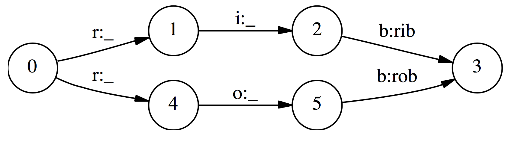
- Given the observation sequence: r i b
In the first time step, r matches both transitions from the start state, so the probability mass gets distributed roughly equally among those two transitions. Next we observe i. Both states 1 and 4 have only one outgoing transition. State 1 has seen this observation often in training, state 4 has almost never seen this observation; but like state 1, state 4 has no choice but to pass all its mass to its single outgoing transition, since it is not generating the observation, only conditioning on it. Thus, states with a single outgoing transition effectively ignore their observations.
The top path and the bottom path will be about equally likely, independently of the observation sequence. If one of the two words is slightly more common in the training set, the transitions out of the start state will slightly prefer its corresponding transition, and that word’s state sequence will always win.
-
Transitions from a given state are competing against each other only.
-
Per state normalization, i.e. sum of transition probability for any state has to sum to 1.
-
MEMM are normalized locally over each observation where the transitions going out from a state compete only against each other, as opposed to all the other transitions in the model.
-
States with a single outgoing transition effectively ignore their observations.
-
Causes bias: states with fewer arcs are preferred.
-
The idea of CRF is to drop this local per state normalization, and replace it by a global per sequence normalization.
-
So, how do we formalize this global normalization? I will try to explain it in the sections that follow.
Undirected Graphical Models
-
A Conditional Random Field can be seen as an undirected graphical model, or Markov Random Field, globally conditioned on \(X\), the random variable representing observation sequence.
-
Lafferty et al. 2001 define a Conditional Random Field as:
-
\(X\) is a random variable over data sequences to be labeled, and \(Y\) is a random variable over corresponding label sequences.
-
The random variables \(X\) and \(Y\) are jointly distributed, but in a discriminative framework we construct a conditional model \(p(Y \mid X)\) from paired observation and label sequences:
-
-
Let \(G = (V , E)\) be a graph such that \(Y = (Y_{v})\ \ v \in V\), so that \(Y\) is indexed by the vertices of \(G\).
-
\((X, Y)\) is a conditional random field when each of the random variables \(Y_{v}\), conditioned on \(X\), obey the Markov property with respect to the graph:
\[P(Y_{v} \mid X, Y_{w}, w \neq v) = P(Y_{v} \mid X, Y_{w}, w \sim v)\]- where \(w \sim v\) means that \(w\) and \(v\) are neighbors in G. Thus, a CRF is a random field globally conditioned on the observation \(X\). This goes already in the direction of what the MEMM doesn’t give us, states globally conditioned on the observation.
-
This graph may have an arbitrary structure as long as it represents the label sequences being modeled, this is also called general Conditional Random Fields.
-
However the simplest and most common graph structured in NLP, which is the one used to model sequences is the one in which the nodes corresponding to elements of \(Y\) form a simple first-order chain, as illustrated in the figure below:
The figure below (taken from Hanna Wallach 2004) shows chain-structured CRFs globally conditioned on X.
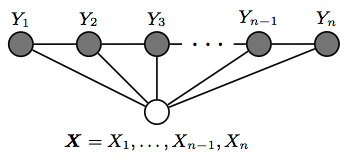
- This is also called linear-chain conditional random fields, which is the type of CRF on which the rest of this post will focus.
Linear-chain CRFs
- Let \(\bar{x}\) is a sequence of words and \(\bar{y}\) a corresponding sequence of \(n\) tags:
-
This can been seen as another log-linear model, but “giant” in the sense that:
- The space of possible values for \(\bar{y}\), i.e., \(Y^{n}\), is huge, where \(n\) is the since of the sequence.
- The normalization constant involves a sum over the set \(Y^{n}\).
-
\(F\) will represent a global feature vector defined by a set of feature functions \(f_{1},...,f_{d}\), where each feature function \(f_{j}\) can analyse the whole \(\bar{x}\) sequence, the current \(y_{i}\) and previous \(y_{i-1}\) positions in the \(\bar{y}\) labels sequence, and the current position \(i\) in the sentence:
-
We can define an arbitrary number of feature functions. The k’th global feature is then computed by summing the \(f_{k}\) over all the \(n\) different state transitions \(\bar{y}\). In this way we have a “global” feature vector that maps the entire sequence: \(F(\bar{x}, \bar{y}) \in {\rm I\!R}^{d}\).
-
Thus, the full expanded linear-chain CRF equation is (figure taken from Sameer Maskey slides):
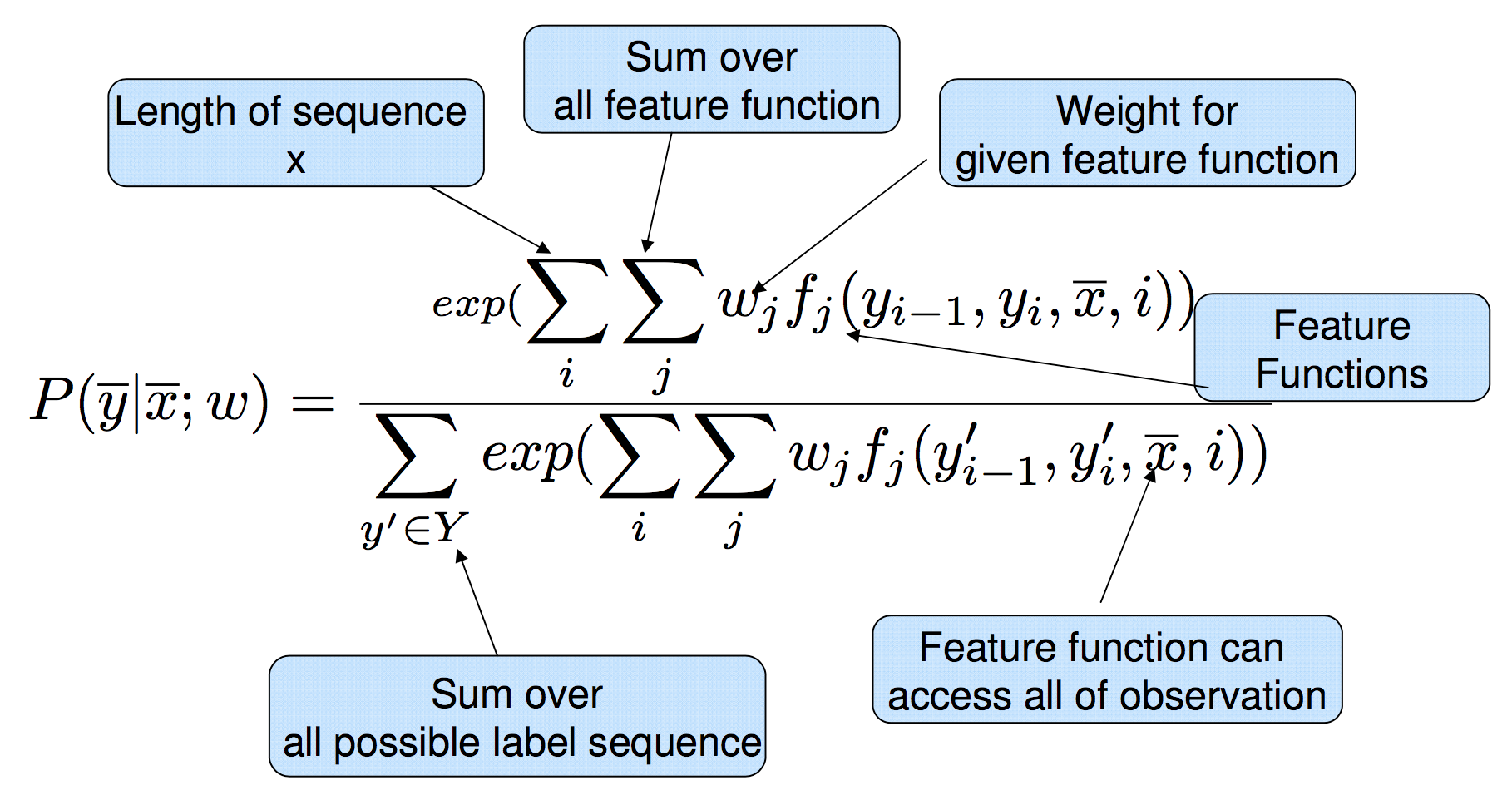
- Having the framework defined by the equation above we now analyze how to perform two operations: parameter estimation and sequence prediction.
Inference
- Inference with a linear-chain CRF resolves to computing the \(\bar{y}\) sequence that maximizes the following equation:
- We want to try all possible \(\bar{y}\) sequences computing for each one the probability of “fitting” the observation \(\bar{x}\) with feature weights \(\bar{w}\). If we just want the score for a particular labelling sequence \(\bar{y}\), we can ignore the exponential inside the numerator, and the denominator:
- Then, we replace \(F(\bar{x},\bar{y})\) by it’s definition:
- Each transition from state \(y_{i-1}\) to state \(y_{i}\) has an associated score:
-
Since we took the \(\exp\) out, this score could be positive or negative, intuitively, this score will be relatively high if the state transition is plausible, relatively low if this transition is implausible.
-
The decoding problem is then to find an entire sequence of states such that the sum of the transition scores is maximized. We can again solve this problem using a variant of the Viterbi algorithm, in a very similar way to the decoding algorithm for HMMs or MEMMs.
-
The denominator, also called the partition function:
\[Z(\bar{x},w)= {\sum\limits_{\bar{y}' \in Y} \exp(\sum\limits_{j} w_{j} F_{j}(\bar{x},\bar{y}'))}\]- … is useful to compute a marginal probability. For example, this is useful for measuring the model’s confidence in it’s predicted labeling over a segment of input. This marginal probability can be computed efficiently using the forward-backward algorithm. See the references section for demonstrations on how this is achieved.
Parameter Estimation
-
We also need to find the \(\bar{w}\) parameters that best fit the training data, a given a set of labelled sentences:
\[\{(\bar{x}_{1}, \bar{y}_{1}), \ldots , (\bar{x}_{m}, \bar{y}_{m})\}\]- where each pair \((\bar{x}_{i}, \bar{y}_{i})\) is a sentence with the corresponding word labels annotated. To find the \(\bar{w}\) parameters that best fit the data we need to maximize the conditional likelihood of the training data:
-
The parameter estimates are computed as:
\[\bar{w}^* = \underset{\bar{w}\ \in {\rm \ I\!R}^{d}} {\arg\max}\ \sum\limits_{i=1}^{m} \log p( \bar{x}_{i} | \bar{y}_{i}, \bar{w}) - \frac{\lambda}{2} \| \bar{w} \| ^{2}\]- where \(\frac{\lambda}{2} \| \bar{w} \| ^{2}\) is an L2 regularization term.
-
The standard approach to finding \(\bar{w}^*\) is to compute the gradient of the objective function, and use the gradient in an optimization algorithm like L-BFGS.
Wrapping up: HMM vs. MEMM vs. CRF
-
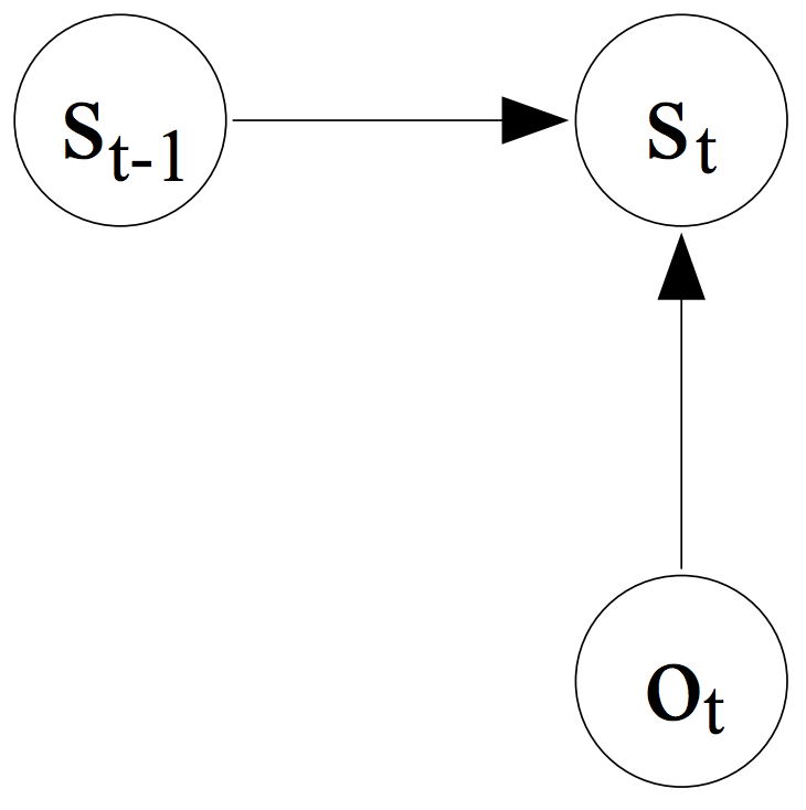
It is now helpful to look at the three sequence prediction models, and compared them. The figure bellow shows the graphical representation for the Hidden Markov Model, the Maximum Entropy Markov Model and the Conditional Random Fields.
-
The figure below (taken from Lafferty et al. 2001) shows the graph representation of HMM, MEMM and CRF:
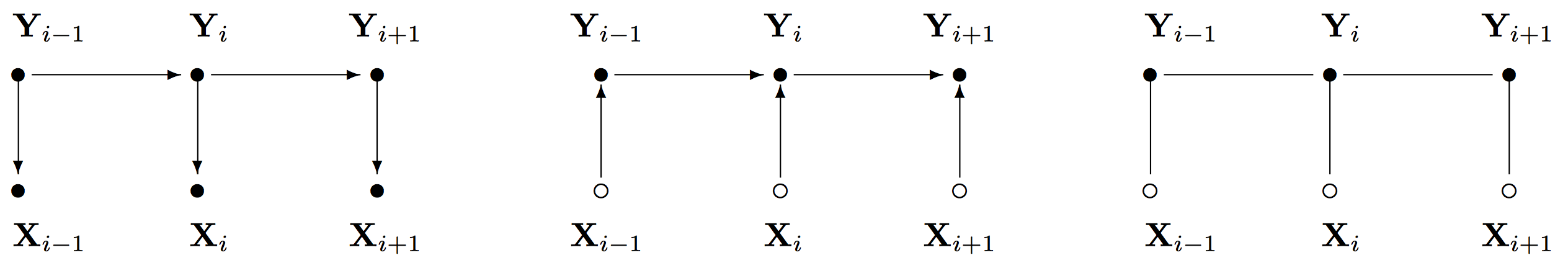
- Hidden Markov Models:
- Maximum Entropy Markov Models:
- Conditional Random Fields:
CRF Important Observations
-
MEMMs are normalized locally over each observation, and hence suffer from the Label Bias problem, where the transitions going out from a state compete only against each other, as opposed to all the other transitions in the model.
-
CRFs avoid the label bias problem a weakness exhibited by Maximum Entropy Markov Models (MEMM). The big difference between MEMM and CRF is that MEMM is locally renormalized and suffers from the label bias problem, while CRFs are globally re-normalized.
-
The inference algorithm in CRF is again based on Viterbi algorithm.
-
Output transition and observation probabilities are not modelled separately.
-
Output transition dependent on the state and the observation as one conditional probability.
Software Packages
-
python-crfsuite: is a python binding for CRFsuite which is a fast implementation of Conditional Random Fields written in C++.
-
CRF++: Yet Another CRF toolkit: is a popular implementation in C++ but as far as I know there are no python bindings.
-
MALLET:includes implementations of widely used sequence algorithms including hidden Markov models (HMMs) and linear chain conditional random fields (CRFs), it’s written in Java.
-
FlexCRFs supports both first-order and second-order Markov CRFs, it’s written in C/C++ using STL library.
-
python-wapiti is a python wrapper for wapiti, a sequence labeling tool with support for maxent models, maximum entropy Markov models and linear-chain CRF.
References
-
“Conditional Random Fields: Probabilistic Models for Segmenting and Labeling Sequence Data”
-
“An Introduction to Conditional Random Fields” Sutton, Charles; McCallum, Andrew (2010)
Citation
If you found our work useful, please cite it as:
@article{Chadha2020DistilledConditionalRandomFields,
  title   = {Conditional Random Fields for Sequence Prediction},
  author  = {Chadha, Aman},
  journal = {Distilled AI},
  year    = {2020},
  note    = {\url{https://aman.ai}}
}