Primers • Autoregressive vs. Autoencoder Models

• Overview: Autoregressive and autoencoder models
• Taxonomy
• Autoregressive/Decoder Models
• How does an Autoregressive Model Work?
• Autoregressive Language Models
• Autoencoder/Encoder Models
• Encoder-Decoder/Seq2seq Models
• Enter XLNet: the best of both worlds
  • Permutation Language Modeling
  • What problems does permutation language modeling bring?
  • Does BERT have the issue of separating position embeddings from the token embeddings?
  • How does XLNet solve the issue of separating position embeddings from token embeddings?
• Attention mask: How does XLNet implement permutation?
• Further Reading
• Citation

Overview: Autoregressive and autoencoder models

• Unsupervised representation learning has been highly successful in the domain of natural language processing. Typically, these methods first pretrain neural networks on large-scale unlabeled text corpora, and then finetune the models or representations on downstream tasks. Under this shared high-level idea, different unsupervised pretraining objectives have been explored in literature.
• Among them, autoregressive (AR) language modeling and autoencoding (AE) have been the two most successful pretraining objectives.
• Tying this in with the Transformer architecture, the Transformer encoder is an AE model while the Transformer decoder is an AR model.

Taxonomy

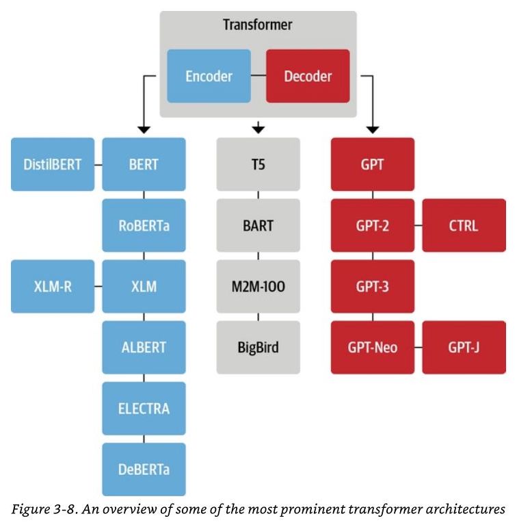
• The following tree diagram (source) shows the Transformer encoders/AE models (blue), Transformer decoders/AR models (red) and Transformer Encoder-Decoder/seq2seq models (grey):

Autoregressive/Decoder Models

• An AR model learns from a series of timed steps and takes measurements from previous actions as inputs for a regression model, in order to predict the value of the next time step.
• AR models are typically used for generation tasks, such as tasks in the domain of natural language generation (NLG), for e.g., such as summarization, translation, or abstractive question answering.

How does an Autoregressive Model Work?

• AR modeling centers on measuring the correlation between observations at previous time steps (the lag variables) to predict the value of the next time step (the output).
• If both variables change in the same direction, for example increasing or decreasing together, then there is a positive correlation. If the variables move in opposite directions as values change, for example one increasing while the other decreases, then this is called negative correlation. Either way, using basic statistics, the correlation between the output and previous variable can be quantified.
• The higher this correlation, positive or negative, the more likely that the past will predict the future. Or in machine learning terms, the higher this value will be weighted during deep learning training.
• Since this correlation is between the variable and itself at previous time steps, it is referred to as an autocorrelation.
• In addition, if every variable shows little to no correlation with the output variable, then its likely that the time series dataset may not be predictable.

Autoregressive Language Models

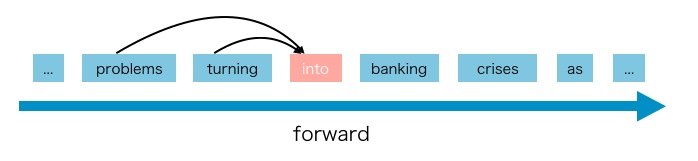
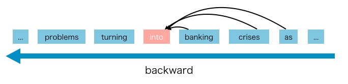
• In language modeling, an AR language model is a kind of model that using the context word to predict the next word by estimating the probability distribution of a text corpus with an autoregressive model. Specifically, given a text sequence \(\mathbf{x}=\left(x_{1}, \cdots, x_{T}\right)\), AR language modeling factorizes the likelihood into a forward product \(p(\mathbf{x})=\prod_{t=1}^{T} p\left(x_{t} \mid \mathbf{x}_{<t}\right)\) or a backward one \(p(\mathbf{x})=\prod_{t=T}^{1} p\left(x_{t} \mid \mathbf{x}_{>t}\right)\).
• A parametric model (e.g. a neural network) is trained to model each conditional distribution. Since an AR language model is only trained to encode a uni-directional context (either forward or backward), it is not effective at modeling deep bidirectional contexts. The figures below (source) illustrates the forward/backward directionality.

• On the contrary, downstream language understanding tasks often require bidirectional context information. This results in a gap between AR language modeling and effective pretraining.
• GPT, GPT-2, GPT-3, and CTRL are examples of AR language models.
• The pros and cons of an AR language model are as follows:
  • Pros:
    • AR language models are good at generative NLP tasks. Since AR models utilize causal attention to predict the next token, they are naturally applicable for generating content. The other advantage of AR models is that generating data for them is relatively easy, since you can simply have the training objective be to predict the next token in a given corpus.
  • Cons:
    • AR language models have some disadvantages, it only can use forward context or backward context, which means it can’t use bidirectional context at the same time.

Autoencoder/Encoder Models

• AE based pretraining does not perform explicit density estimation but instead aims to reconstruct the original data from corrupted input (“fill in the blanks”).
• AE models are typically used for content understanding tasks, such as tasks in the domain of natural language understanding (NLU) that involve classification, for e.g., sentiment analysis, or extractive question answering.
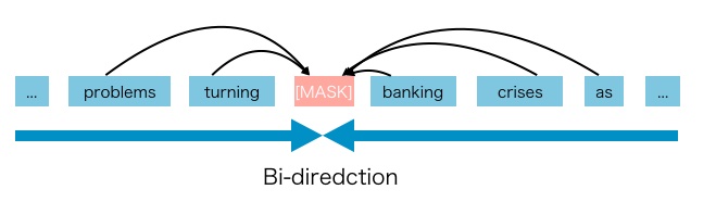
• A notable example is BERT, which has been the state-of-the-art pretraining approach. Given the input token sequence, a certain portion of tokens are replaced by a special symbol [MASK], and the model is trained to recover the original tokens from the corrupted version. The AE language model aims to reconstruct the original data from corrupted input.
• Since density estimation is not part of the objective, BERT is allowed to utilize bidirectional contexts for reconstruction. As an immediate benefit, this closes the aforementioned bidirectional information gap in AR language modeling, leading to improved performance. However, the artificial symbols like [MASK] used by BERT during pretraining are absent from real data at finetuning time, resulting in a pretrain-finetune discrepancy. Moreover, since the predicted tokens are masked in the input, BERT is not able to model the joint probability using the product rule as in AR language modeling. In other words, BERT assumes the predicted tokens are independent of each other given the unmasked tokens, which is oversimplified as high-order, long-range dependency is prevalent in natural language.

• With masked language modeling as a common training objective in pre-training autoencoder models, we predict the value of the original value of the masked tokens in the corrupted input.
• BERT (and all of its variants such as RoBERTa, DistilBERT, ALBERT, etc.), XLM are examples of AE models.
• The pros and cons of an AE model are as follows:
  • Pros:
    • Context dependency: The AR representation \(h_{\theta}\left(\mathbf{x}_{1: t-1}\right)\) is only conditioned on the tokens up to position \(t\) (i.e. tokens to the left), while the BERT representation \(H_{\theta}(\mathbf{x})_{t}\) has access to the contextual information on both sides. As a result, the BERT objective allows the model to be pretrained to better capture bidirectional context.
  • Cons:
    • Input noise: The input to BERT contains artificial symbols like [MASK] that never occur in downstream tasks, which creates a pretrain-finetune discrepancy. Replacing [MASK] with original tokens as in [10] does not solve the problem because original tokens can be only used with a small probability - otherwise Eq. (2) will be trivial to optimize. In comparison, AR language modeling does not rely on any input corruption and does not suffer from this issue. Put simply, AE models use the [MASK] token during the pretraining, but these symbols are absent from real-world data during finetuning time, resulting in a pretrain-finetune discrepancy.
    • Independence Assumption: As emphasized by the \(\approx\) sign in Eq. (2), BERT factorizes the joint conditional probability \(p(\overline{\mathbf{x}} \mid \hat{\mathbf{x}})\) based on an independence assumption that all masked tokens \(\overline{\mathbf{x}}\) are separately reconstructed. In comparison, the AR language modeling objective (1) factorizes \(p_{\theta}(\mathbf{x})\) using the product rule that holds universally without such an independence assumption. Put simply, another disadvantage of [MASK] is that it assumes the predicted (masked) tokens are independent of each other given the unmasked tokens. For example, consider a sentence: “it shows that the housing crisis was turned into a banking crisis”. If we mask “banking” and “crisis”, the masked words contain an implicit relation to each other. But the AE model is trying to predict “banking” given unmasked tokens, and predict “crisis” given unmasked tokens separately. It ignores the relation between “banking” and “crisis”. In other words, it assumes the predicted (masked) tokens are independent of each other. The model should learn such correlation among the predicted (masked) tokens to predict one of the tokens.

Encoder-Decoder/Seq2seq Models

• An encoder-decoder/seq2seq model, as the name suggests, uses both an encoder and decoder. It treats each task as sequence to sequence conversion/generation (for e.g., text to text, or even multimodal tasks such as text to image or image to text). For instance, for text classification, the encoder takes text as input, and the decoder generates text labels instead of classifying them.
• Encoder-decoder/seq2seq models are typically used for tasks that require both content understanding and generation (where the content needs to be converted from one form to another), such as machine translation.
• T5, BART, and BigBird are examples of Encoder-Decoder models.

Enter XLNet: the best of both worlds

• XLNet is an example of a generalized autoregressive pretraining method, which leverages the best of both AR language modeling and AE while avoiding their limitations, i.e., it offers an AR language model which utilizes bi-directional context and avoids the independence assumption and pretrain-finetune discrepancy disadvantages brought by the token masking method in AE models.

Permutation Language Modeling

• The AR language model only can use the context either forward or backward, so how to let it learn from bi-directional context?
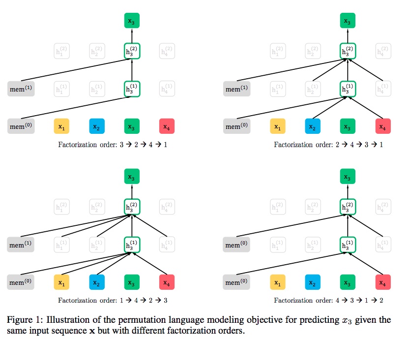
• Language model consists of two phases, the pre-train phase, and fine-tune phase. XLNet focus on pre-train phase. In the pre-train phase, it proposed a new objective called Permutation Language Modeling. We can know the basic idea from this name, it uses permutation. The following Illustration from the paper (source) shows the idea of permutation:

• Here’s an example. The sequence order is \([x_1, x_2, x_3, x_4]\). All permutations of such sequence are below.

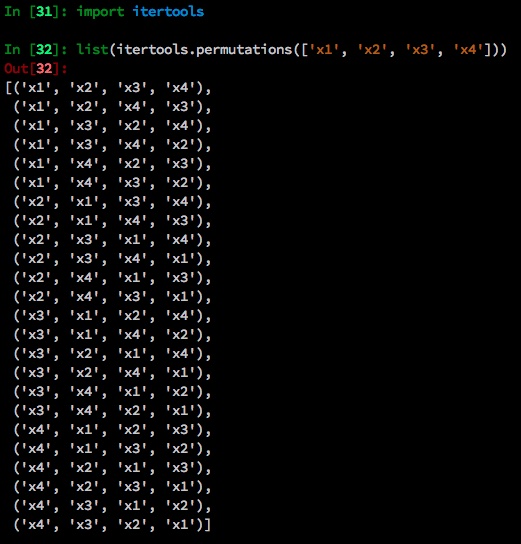
• For these four tokens (\(N\)) in the input sentence, there are 24 (\(N!\)) permutations.
• The scenario is that we want to predict the \(x_3\). So there are 4 patterns in the 24 permutations where \(x_3\) is at the first, second, third, and fourth position, as shown below and summarized in the figure below (source).

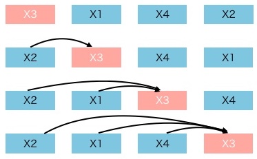
• Here we set the position of \(x_3\) as the \(t^{th}\) position and the remaining \(t-1\) tokens are the context words for predicting \(x_3\). Intuitively, the model will learn to gather bi-directional information from all positions on both sides.

What problems does permutation language modeling bring?

• The permutation can make AR model see the context from two directions, but it also brought problems that the original transformer cannot solve. The permutation language modeling objective is as follows:

  \[\max _{\theta} \mathbb{E}_{\mathbf{z} \sim \mathcal{Z}_{T}}\left[\sum_{t=1}^{T} \log p_{\theta}\left(x_{z_{t}} \mid \mathbf{x}_{\mathbf{z}_{<t}}\right)\right]\]
  • where,
    • \(Z\): a factorization order
    • \(p_θ\): likelihood function
    • \(x_zt\): the \(t^{th}\) token in the factorization order
    • \(x_z<t\): the tokens before \(t^{th}\) token
• This is the objective function for permutation language modeling, which means takes \(t-1\) tokens as the context and to predict the \(t^{th}\) token.
• There are two requirements that a standard Transformer cannot do:
  • to predict the token \(x_t\), the model should only see the position of \(x_t\), not the content of \(x_t\).
  • to predict the token \(x_t\), the model should encode all tokens before \(x_t\) as the content.
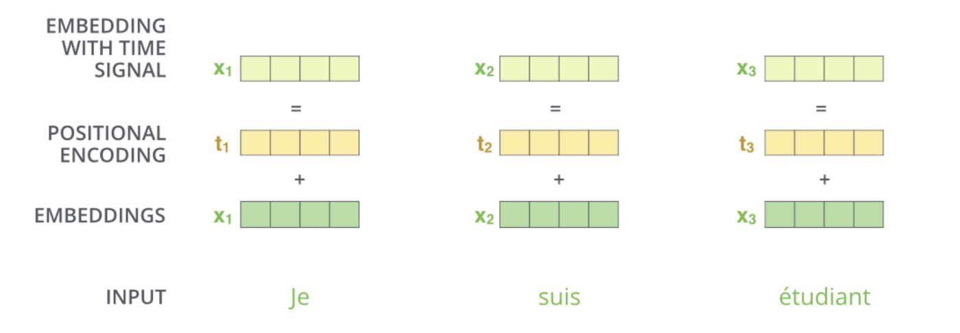
• Considering the first requirement above, BERT amalgamates the positional encoding with the token embedding (c.f. figure below; source), and thus cannot separate the position information from the token embedding.

Does BERT have the issue of separating position embeddings from the token embeddings?

• BERT is an AE language model, it does not need separate position information like the AR language model. Unlike the XLNet need position information to predict \(t^{th}\) token, BERT uses [MASK] to represent which token to predict (we can think [MASK] is just a placeholder). For example, if BERT uses \(x_2\), \(x_1\) and \(x_4\) to predict \(x_3\), the embedding of \(x_2\), \(x_1\), \(x_4\) contains the position information and other information related to [MASK]. So the model has a high chance to predict that [MASK] is \(x_3\).

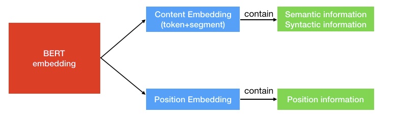
• BERT embeddings contain two types of information, the positional embeddings, and the token/content embeddings (here, we’re skipping the sequence embeddings since we’re not concerned about the next sentence prediction (NSP) task), as shown in the figure below (source).

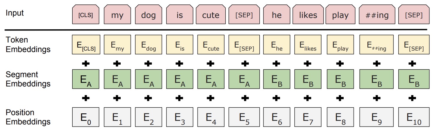
• The position information is easy to understand that it tells the model the position of the current token. The content information (semantics and syntactic) contains the “meaning” of the current token, as shown in the figure below (source):

• An intuitive example of relationships learned with embeddings from the Word2Vec paper is:

How does XLNet solve the issue of separating position embeddings from token embeddings?

• As shown in the figure below (source), XLNet proposes two-stream self-attention to solve the problem.

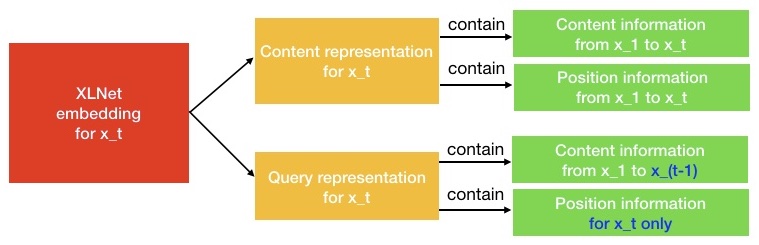
• As the name indicates, it contains two kinds of self-attention. One is the content stream attention, which is the standard self-attention in Transformer. The other one is the query stream attention. XLNet introduces it to replace the [MASK] token in BERT.
• For example, if BERT wants to predict \(x_3\) with knowledge of the context words \(x_1\) and \(x_2\), it can use [MASK] to represent the \(x_3\) token. The [MASK] is just a placeholder. And the embedding of \(x_1\) and \(x_2\) contains the position information to help the model to “know” [MASK] is \(x_3\).
• Things are different come to XLNet. One token \(x_3\) will serve two kinds of roles. When it is used as content to predict other tokens, we can use the content representation (learned by content stream attention) to represent \(x_3\). But if we want to predict \(x_3\), we should only know its position and not its content. That’s why XLNet uses query representation (learned by query stream attention) to preserve context information before \(x_3\) and only the position information of \(x_3\).
• In order to intuitively understand the Two-Stream Self-Attention, we can just think XLNet replace the [MASK] in BERT with query representation. They just choose different approaches to do the same thing.

Attention mask: How does XLNet implement permutation?

• The following shows the various permutations that a sentence \([x_1, x_2, x_3, x_4]\) can take:

• It is very easy to misunderstand that we need to get the random order of a sentence and input it into the model. But this is not true. The order of input sentence is \([x_1, x_2, x_3, x_4]\), and XLNet uses the attention mask to permute the factorization order, as shown in the figure (source) below.

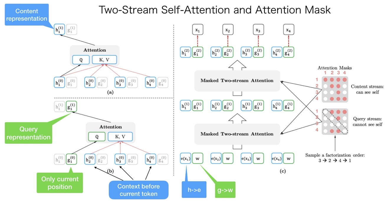
• From the figure above, the original order of the sentence is \([x_1, x_2, x_3, x_4]\). And we randomly get a factorization order as \([x_3, x_2, x_4, x_1]\).
• The upper left corner is the calculation of content representation. If we want to predict the content representation of \(x_1\), we should have token content information from all four tokens. \(K_V = [h_1, h_2, h_3, h_4]\) and \(Q = h_1\).
• The lower-left corner is the calculation of query representation. If we want to predict the query representation of \(x_1\), we cannot see the content representation of \(x_1\) itself. \(K_V = [h_2, h_3, h_4]\) and \(Q = g_1\).
• The right corner is the entire calculation process. Let’s do a walk-through of it from bottom to top. First, \(h(\cdot)\) and \(g(\cdot)\) are initialized as \(e(x_i)\) and \(w\). And after the content mask and query mask, the two-stream attention will output the first layer output \(h^{(1)}\) and \(g^{(1)}\) and then calculate the second layer.
• Notice the right content mask and query mask. Both of them are matrices. In the content mask, the first row has 4 red points. It means that the first token (\(x_1\)) can see (attend to) all other tokens including itself (\(x_3 \rightarrow x_2 \rightarrow x_4 \rightarrow x_1\)). The second row has two red points. It means that the second token (\(x_2\)) can see (attend to) two tokens (\(x_3 \rightarrow x_2\)). And so on other rows.
• The only difference between the content mask and query mask is those diagonal elements in the query mask are 0, which means the tokens cannot see themselves.
• To sum it up: the input sentence has only one order. But we can use different attention mask to implement different factorization orders.

Further Reading

• Transformer Text Embeddings
• what is the first input to the decoder in a transformer model?
• What are the inputs to the first decoder layer in a Transformer model during the training phase?

Citation

If you found our work useful, please cite it as:

@article{Chadha2020DistilledAutoregressiveVSAutoencoders,
  title   = {Autoregressive vs. Autoencoder Models},
  author  = {Chadha, Aman},
  journal = {Distilled AI},
  year    = {2020},
  note    = {\url{https://aman.ai}}
}