CS231n • Detection and Segmentation
- Review: (Unsupervised) Generative Models
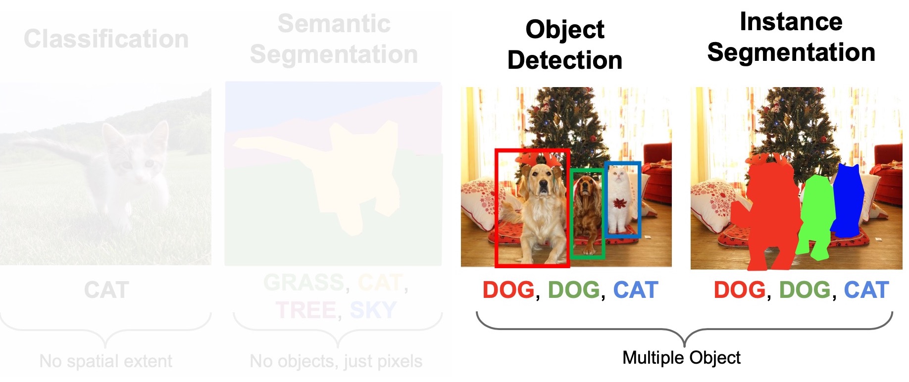
- Image Classification
- Semantic Segmentation
- Single Object Detection (Localization + Classification)
- Multiple Object Detection
- Region Proposals: Selective Search
- R-CNN
- Fast R-CNN
- Faster R-CNN
- Region of Interest (RoI) Align
- One stage vs. two stage object detector
- Object Detection: Summary
- Instance Segmentation
- Open Source Frameworks
- Beyond 2D Object Detection
- Key Takeaways
- Citation
Review: (Unsupervised) Generative Models
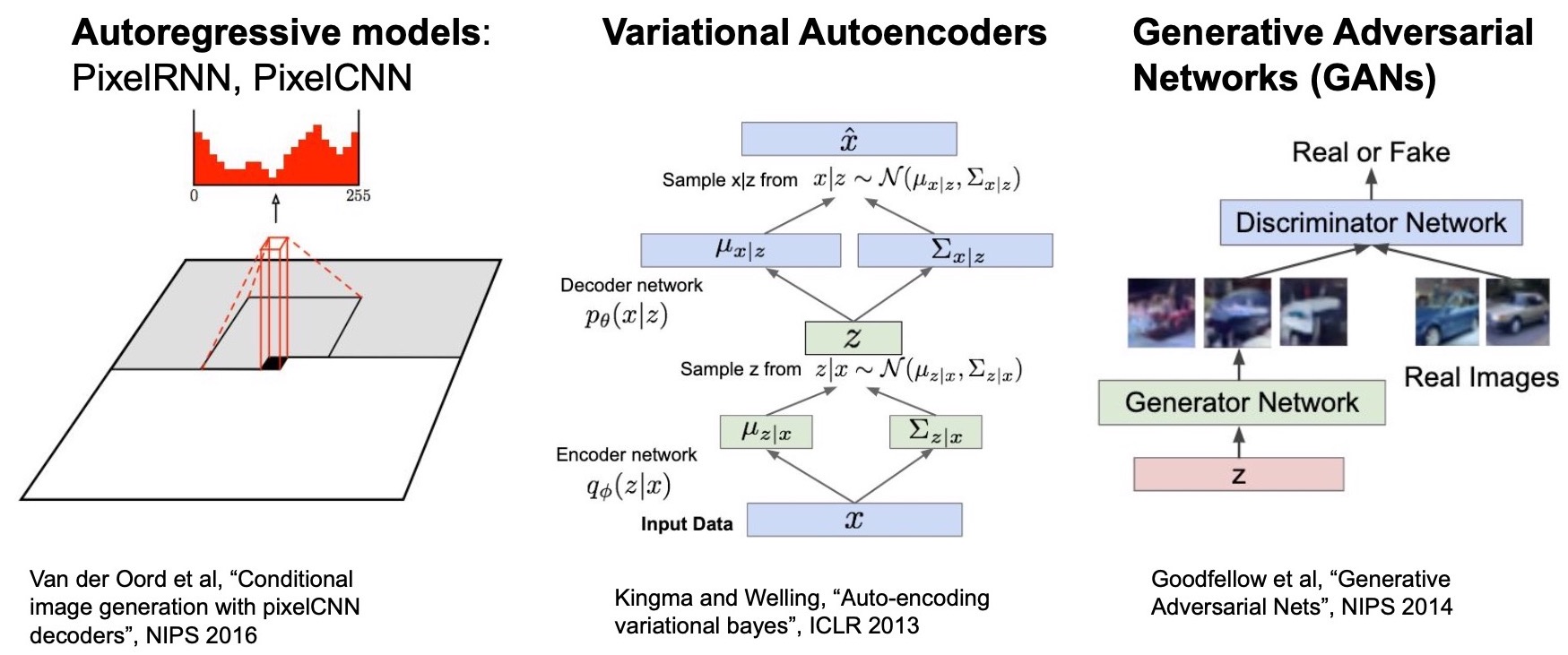
- In “Generative Models”, we talked about PixelRNN and PixelCNN which are both auto-regressive models (i.e., they generate a pixel at a time using previously generated pixels) and explicitly model the density likelihood function (“explicit density models”). Both define and optimize a tractable likelihood function. However, a clear downside of such methods is that pixel generation is sequential and thus very slow at test time.
- Next, we talked about Variational AutoEncoders (VAEs) which introduced the latent variable \(z\) and defined a conditional distribution \(p(x | z)\) for modeling the data likelihood.
- Recall that intuitively, \(z\) refers to meaningful Factors of Variations (FoVs). For e.g., if we’re modeling images of human faces, then the dimensions of \(z\) can imply degrees of smile or head pose orientation, etc.
- We then came up with an expression of the data likelihood function over the conditional distribution by marginalizing over \(z\).
- However, the likelihood function is intractable to optimize, so we derived the Evidence LowerBOund (ELBO) on the likelihood expression and maximized the lower bound to indirectly maximize the data likelihood expression.
- The brute (re-)parameterization trick help us differentiate through sampling the approximate posterior and allows us to train the entire VAE model end-to-end.
- Finally, we talked about Generative Adversarial Networks (GANs) which learn to generate new images without defining a likelihood function.
- This involves formulating a two-player game between the generator and the discriminator to tell if the generated image is real or fake.
- The generator uses the real or fake signal from the discriminator to improve its generative samples and thus, improve the “naturality” of the generated images.
- The discriminator, in turn, learns to update its decision boundary to better model the training distribution.
- Lastly, we formally defined the training objective of minimax GAN between the two neural networks and talked about how to train the networks iteratively.
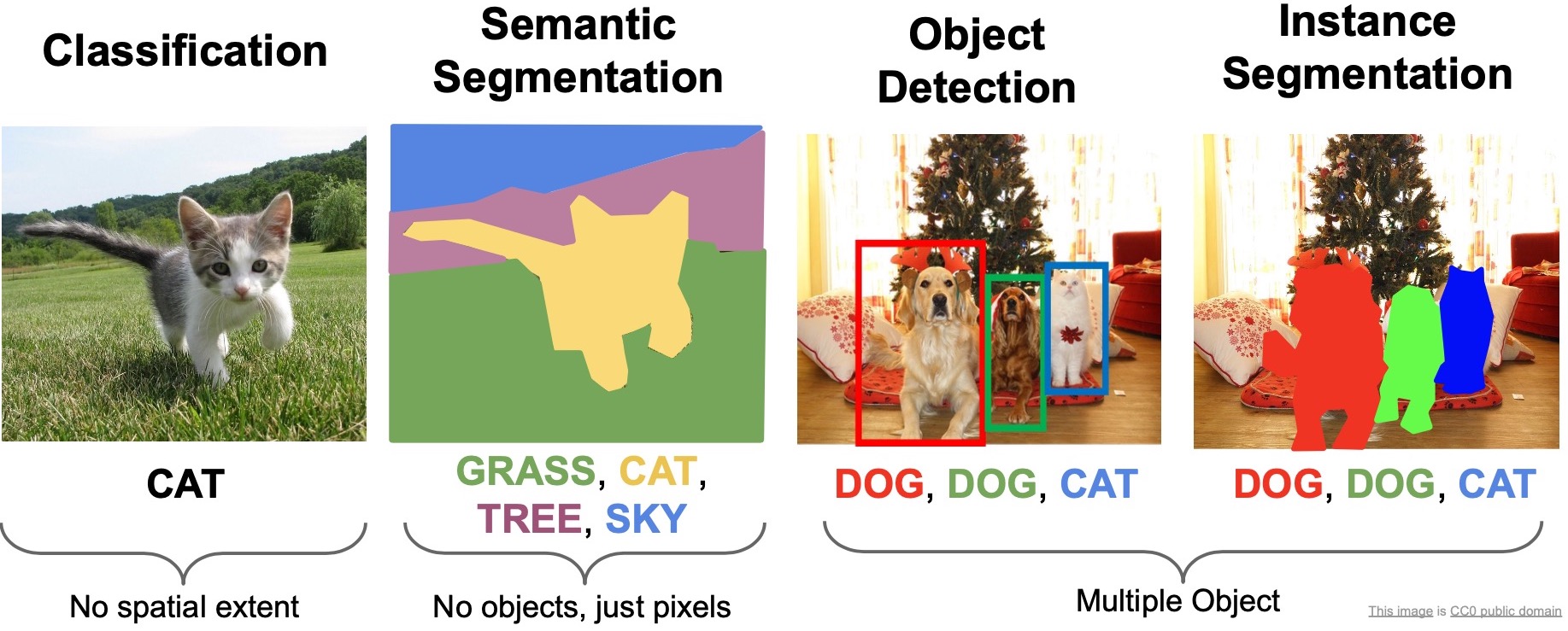
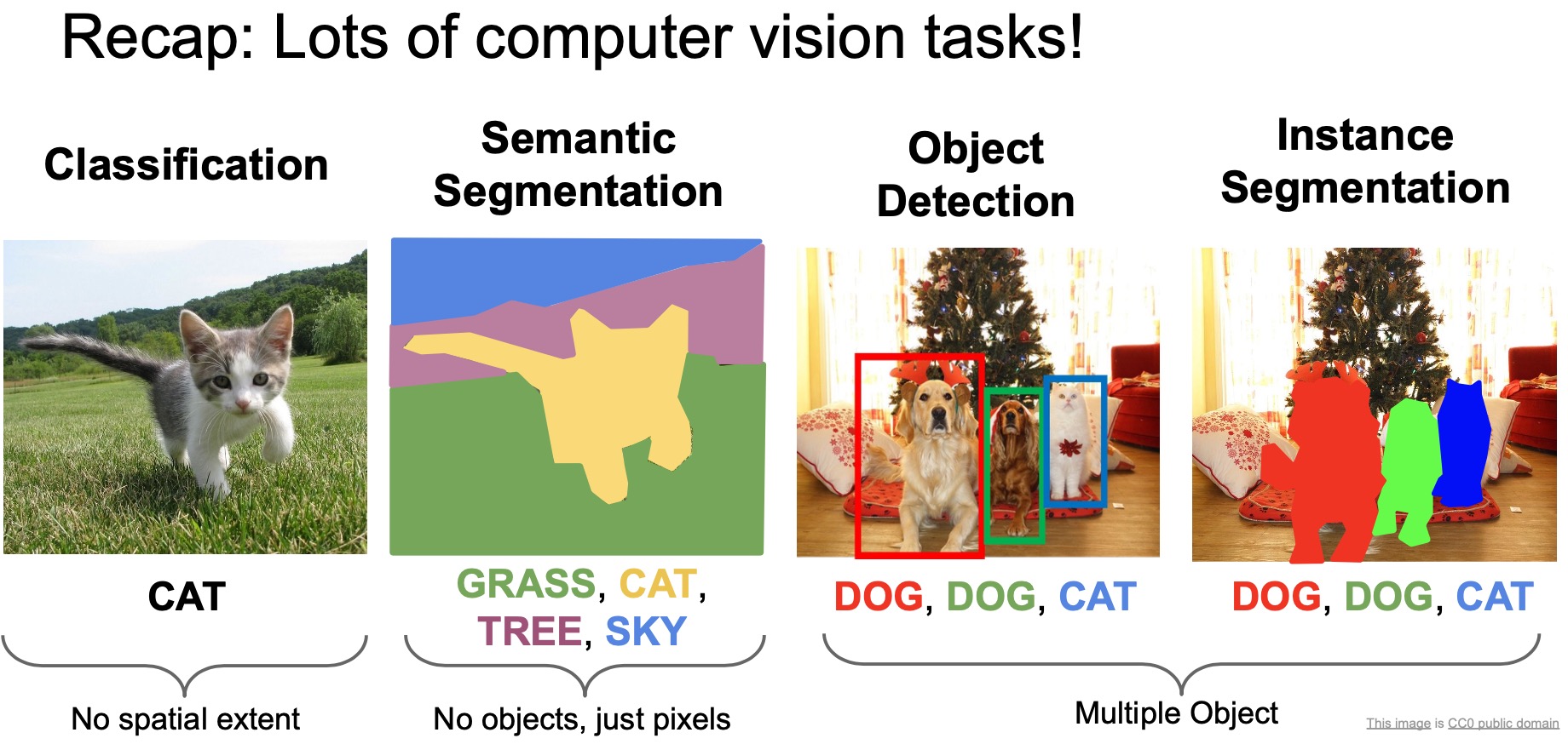
- Thus far, we’ve talked about the image classification problem. In this section, we will talk about (i) segmentation (semantic, instance) and, (ii) object localization and detection (or simply, “object detection”).
Image Classification
- Recall that for the image classification task, our goal is is to predict the semantic categories of the (only) object in the image.
- Offers a very coarse description of the scene.
- Basically, we’re summarizing the entire picture using a single word.
- In real world applications, you often want fine grained descriptions of the scene, which the tasks of semantic segmentation, object detection and instance segmentation offer.
- The intuitions we’ve developed about ConvNets in previous topics can be directly applied to the harder problems of segmentation and detection.
Semantic Segmentation
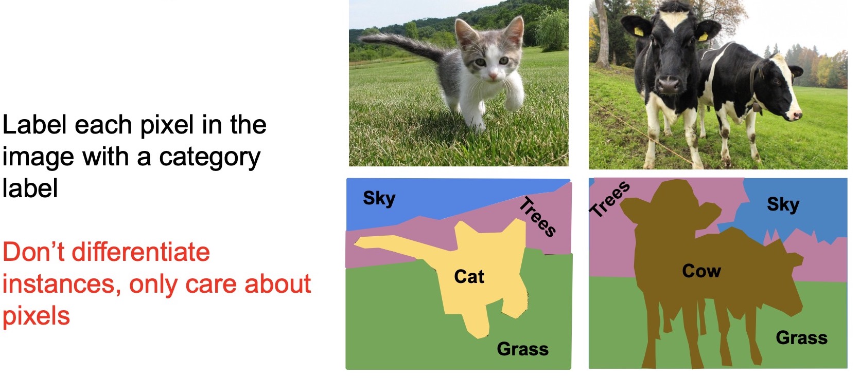
- The goal is to model a very fine grained description of the scene, i.e., at the pixel level. In other words, we’re looking to classify the semantic categories for every single pixel in the image. Note that semantic segmentation has no notion of objects (or instances) in the image – rather, the input quantum that it works on is the pixel.
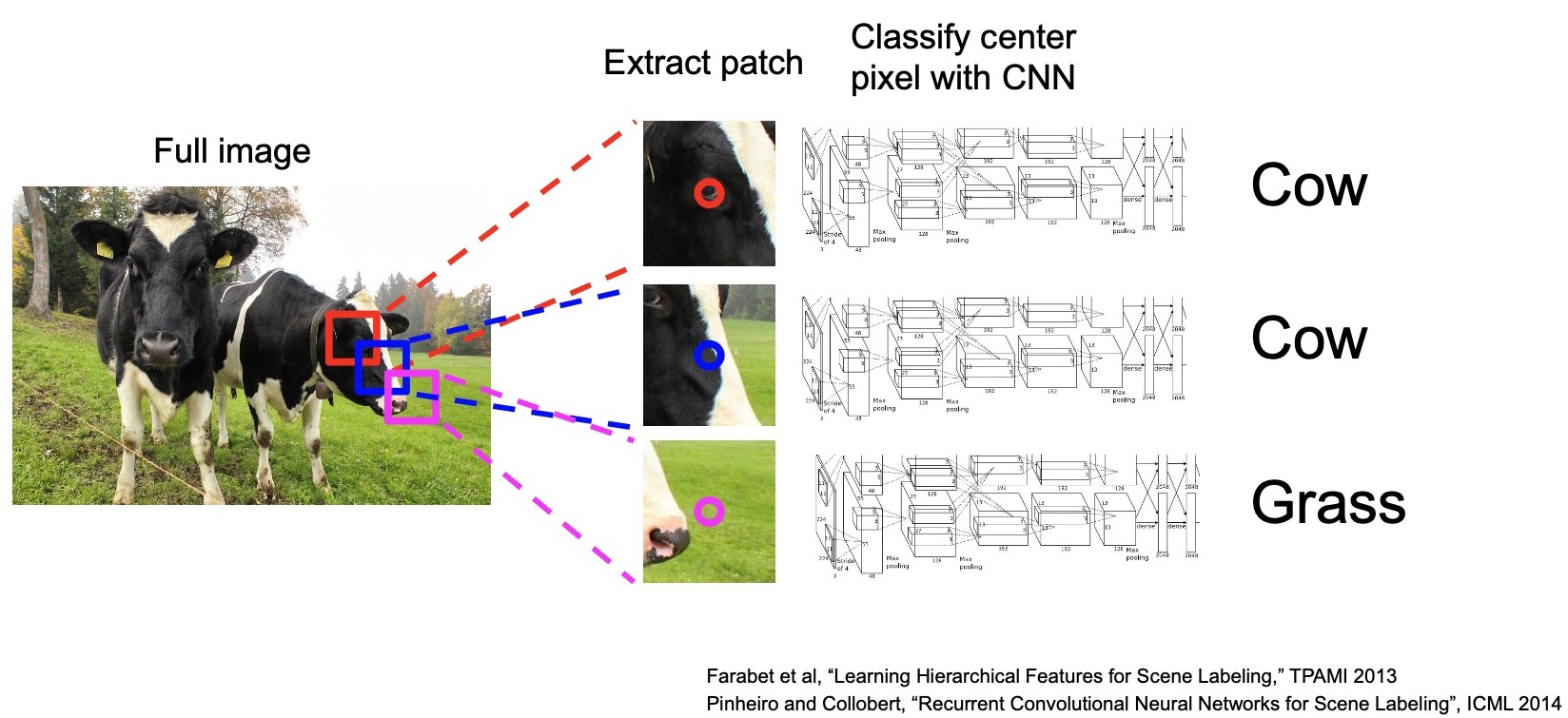
- However, using a single pixel and performing classification on the pixel is an extremely difficult problem even for us humans because a single RGB pixel lacks content.
- To work past this issue, we seek to include context to classify pixels. The simplest form of context is the region around the pixel.
- Take a crop around the pixel and treat the crop as a the context for classifying the center pixel.
Sliding window
- The next question is: how do we modeling this as a learning problem?
- The first idea is to use a sliding window approach. This simple idea uses the same object classification convolutional architecture that we have learned before and treat each crop as an input image to the classifier.
- Recall that we have access to the pixel-wise semantic category labels so we can train this model easily with standard classification loss.
- This approach is known as the sliding window approach for semantic segmentation because we’re sliding a fixed size window over the entire image for cropping image patches.
- The model assigns a label to the center pixel for each window.
- (-) Computationally expensive:
- The sliding-window semantic segmentation approach was popular before 2014. However, it is computationally expensive. To segment an image, we need to do as many forward passes through the model as the number of pixels in the image to predict all the pixels in an image. For instance, for a \(640 \times 480\) image = \(300K\) forward passes.
- So how do we make the sliding window approach faster?
- One observation we can make is that the features generated from the model will have a lot of overlap if we do the sliding window approach, especially for the neighboring windows.
- When we move the sliding window by one pixel, most of the input pixels from the previous window will be in the new window. The same pixels will go through the Conv filters for multiple sliding windows.
- Repeated Conv operations are essentially wasted. The sliding window approach is thus very inefficient since we are not reusing shared features between overlapping patches. Therefore, in practice nobody uses this approach.
Convolution
- (+) How do we encourage the model to reuse the features in order to reduce the amount of wasted compute?
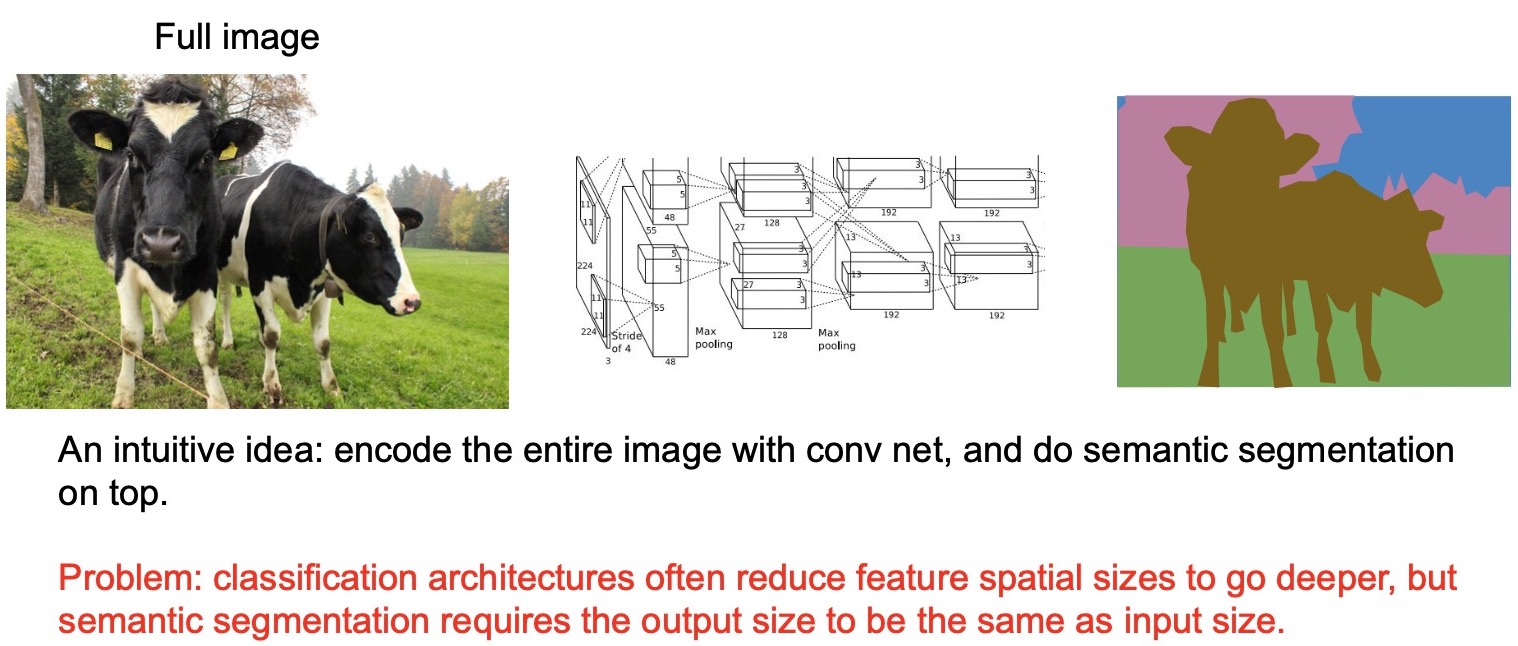
- An intuitive idea is that maybe we can pass an entire image, extract features and perform semantic segmentation on top of these features, thus outputting a segmentation “map” for the entire image.
- (-) Network output size mismatches the input size: An issue with this approach is that we cannot just use a standard classification architecture such as AlexNet or VGGnet because they reduce the feature spatial sizes, with say max pooling or strided convolutions (stride > 1), to go deeper which is how they construct a super deep model. Semantic segmentation requires the size of the output of the network to be the same as the input size, so that each output pixel corresponds to the label of each corresponding input pixel. This is where the Fully Convolutional Networks (FCNs) come in.
Fully Convolutional Architectures
- We can design a network with only convolutional layers and remove all of the sub-sampling operators such as max pooling or strided convolutions such that the output features spatial size is the same as the input image size. In other words, our input is the entire image and our output is the image with each pixel labeled.
- Each layer, thus, will only change the number of channels and keep the spatial dimensions of the features the same.
- Consider a \(3 \times H \times W\) image (note the channel-first notation) shown below:
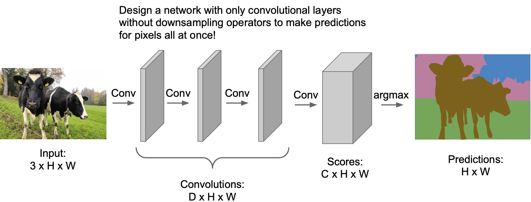
- Passing this image through the conv layers, only the channel size \(D\) will change, but will keep the spatial dimensions \(H\) and \(W\) the same.
- This will lead to scores over \(C\) possible classes. The output “channel” size of the last conv layer is of size \(C\) (\(C \times H \times W\)), i.e., output size = input size.
- We can thus treat output of the last conv layer to be the pixel-wise classification (since each input pixel now has a corresponding output with class probabilities over \(C\) classes). We take the argmax over the class probabilities to find the most probable class according to the model out of the \(C\) options.
- This is very similar to what we had for object classification and the only difference is that instead of just making one prediction for the image, we’re making a prediction for all the pixels all at once!
- Training such a model is very easy – we can train it with pixel-wise classification cross-entropy loss.
- (+) Share features and do not have to perform a forward pass for each sliding window. Recall how convolution works – each entry in the conv activation map is operated on by all of the filters in the next conv layers to generate the activation maps for the next layer. The fully convolutional architecture allows features to be re-used/shared and generate the predictions for all the pixels all at once. Compare and contrast this with the sliding window approach, this approach has its merits as you can share features and do not have to perform a forward pass for each sliding window.
- (-) Doing conv at the original image resolution is very expensive. Especially true for very deep models. Recall that when we discussed the VGG network, we talked about the amount of compute each layer requires and the compute bottleneck is actually at the early layers because these layers are doing convolutions at the original image size so thats quite expensive. This is why, downsampling is needed to reduce the feature size to go deeper. For this reason, you will almost never see this kind of a fully convolutional apporach used in practice.
- Now, the next question is: how do we construct a deep model that has the same input and output feature dimensions and at the same time, one that is also computationally efficient.
Downsampling and upsampling using Fully Convolutional Architectures
- The third idea is based on the last idea and builds upon it. The difference is that we are downsampling and upsampling inside the network.
- The network has two stages: (i) downsampling and (ii) upsampling.
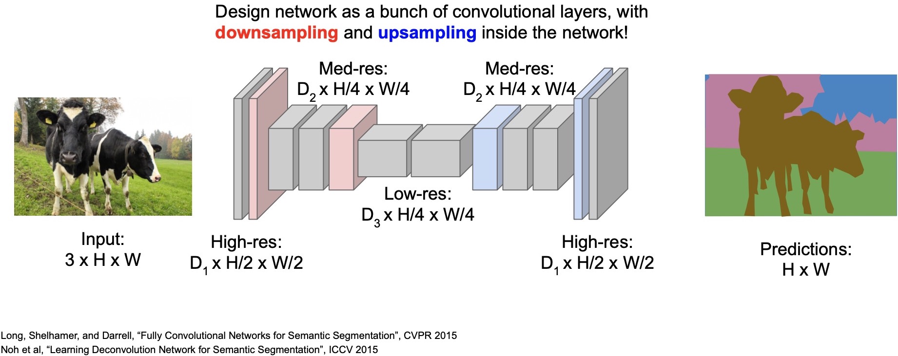
- Downsampling helps save compute by reducing the feature dimension size and thus, allows us to go deeper. On the other hand, upsampling is needed so our output size matches the input size.
- Once the features are of a sufficiently low resolution, we enter the upsampling stage and use the upsampling operators to scale the features back to the original image size.
- So, in this example we see here, we start with an image of size \(3 \times H \times W\) and in the downsampling stage, reduce the dimensions to \(D2 \times H/4 \times W/4\). The upsampling stage scales it back to the original image size.
- (+) Obviates the need to perform convolution at the original image resolution: By using the up and downsampling stages, we can build computationally efficient deep models with the same input and output spatial dimension sizes. Infact, the most common architectures that perform semantic segmentation utilize such up and downsampling stages.
- Downsampling is accomplishable using typical downsampling operators such as various types of pooling (max, average), strided convolutions, etc. which is what typical classification architectures deploy.
Upsampling with no learnable parameters
- The goal of an upsampling operator is to increase the feature’s spatial dimension size, for e.g., go from a \(2 \times 2\) feature to a \(4 \times 4\) feature. We are ignoring the channel length here because up-/downsampling operator do not sample “across” channels and thus the number of channels is of no relevance here.
- The upsampling operation is thus the opposite of what the downsampling operator involves.
- Unpooling: The most straight-forward upsampling operation is called the “unpooling” operation. There are two ways to accomplish unpooling. The first is the “Nearest Neighbor” approach where you simply repeat values to form a larger feature map. Repeating is differentiable so doing backprop through the operation is possible.
-
“Bed of Nails”: Because you’re essentially putting in nails on a flat tensor :) You scale up features by putting in zeros around the values in the input tensor to construct the output tensor. And these zeros are considered as input similar to zero-padding and will not contribute to the gradient when backpropagating to previous layers, but again, the entire operation is differentiable.
- Nearest Neighbor example:
-
Input:   1  2               Output:   1  1  2  2
(2 x 2)  3  4               (4 x 4)   1  1  2  2
                                      3  3  4  4
                                      3  3  4  4
-
- Bed of Nails example:
-
Input:   1  2               Output:   1  0  2  0
(2 x 2)  3  4               (4 x 4)   0  0  0  0
                                      3  0  4  0
                                      0  0  0  0
-
Max Unpooling
- Another type of upsampling operator is max unpooling. This operation is intended to undo the effect of max pooling. Recall that with max pooling, we lose spatial information by taking the max of a region. For e.g., if we do \(2 \times 2\) max pooling with a stride of 2, the subsequent activation would only be the max value and does not contain information about where this max value comes from out of the 4 possible locations in the previous activation map. We can recover this information by doing max unpooling in the upsampling stage.
- To perform max unpooling, we construct a symmetric architecture shown below where the down- and upsampling stages are completely symmetric in terms of the layer size and each downsampling layer has a corresponding upsampling layer. For each downsampling max pooling layer, we will save the position of the max value. We can then recover the location of this activation at the corresponding unpooling layer, for e.g., using bed-of-nails.
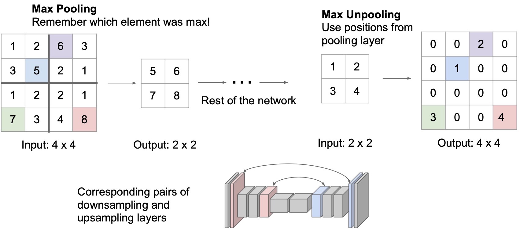
- (+) Recording the output activation’s location during max pooling helps task accuracy: Instead of just assigning values to the upper-left pixel, we’ll assign the activation to the recorded location. So we are essentially undoing max pooling. An intuitive explanation as to why max unpooling is particularly useful for semantic segmentation is that the feature pixels that have the max activation is the most representative pixel in that region, which implies that it holds important information. Assigning the input pixel to the original location in the upsampling stage is helpful for inferring the values of other neighboring pixels in subsequent convolutional layers. This helps with the accuracy of the semantic segmentation task.
Note that the above upsampling operators we reviewed (nearest neighbor, bed-of-nails, max unpooling) have no learnable parameters.
Transpose convolutions (“learnable upsampling” / “ConvT”)
- An upsampling operator with learnable parameters. Widely deployed in practice as the operator of choice for upsampling.
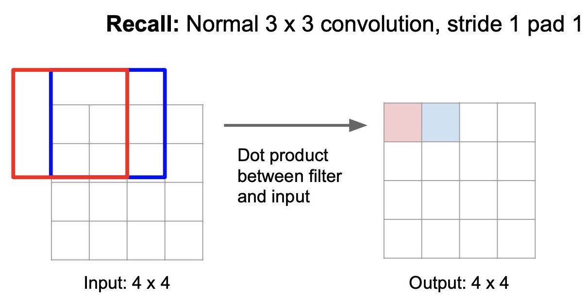
- Recall how convolution works by sliding a convolutional kernel on the image to generate an output feature map. In this case, we’re selecting our stride and padding parameters to have our output spatial size match our input spatial size (by using a stride of 1 and padding of 1 or “same” padding). We generate features from the first window by doing a dot-product between the kernel and the input feature and generate one feature in the output activation map. We then slide the window and generate activations for the second pixel (shown below).
When we increase the stride of the convolutional operation to 2, this effectively downsamples the image. This is because with a stride of 2, the first feature is generated the same way but the second pixel is generated by skipping one pixel and the kernel now moves two steps away from the original kernel’s position (cf. image below).
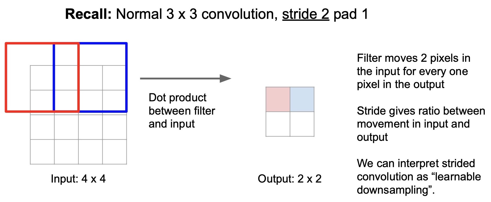
- In a way, we can interpret strided convolutions as learnable downsampling because the convolutional filters have learnable parameters. To clarify, the number of skips we do does not adapt, but these parameters are trainable as opposed to say max pooling, where there’s no learnable parameters.
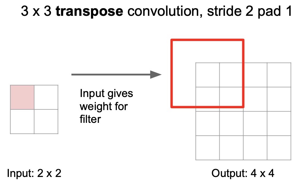
- The direct opposite counterpart of learning to do downsampling with strided convolutions is to learn to do upsampling with the strided transpose convolutions.
- Consider an example of upsampling an input \(2 \times 2\) feature map to a larger feature map of size \(4 \times 4\) with a \(3 \times 3\) transpose convolution with a stride of 2 and padding of 1. The idea behind strided transpose convolutions is to learn to fill the larger activation map with convolution. Similar to vanilla convolutions, we have a \(3 \times 3\) learnable filter (kernel), but instead of doing a dot product between an input pixel patch and the kernel to produce one activation value in the output map, transpose convolution seeks to multiply this \(3 \times 3\) filter with a single pixel in the input feature map to generate a new \(3 \times 3\) tensor which is used to fill up a \(3 \times 3\) region in the larger output activation map (shown by the red region in the diagram below). Note that since we have a padding of 1, the red region has an incomplete coverage of the \(3 \times 3\) region.
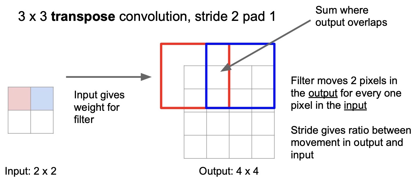
- Next, because we are doing a stride of 2, we will move two steps in the output region and generate a \(3 \times 3\) tensor to fill up the blue region (shown below). This is very similar to strided convolution but instead of taking steps in the input tensor, we’re taking steps in the output tensor.
- Note that for any output feature location with an overlap between two regions/windows, we sum up the values. Since the red and blue regions overlap across 2 pixels, we’ll just add up these values in the output tensor (shown below). This operation continues until the entire output activation map is filled. This explains the inner working of transpose convolutions.
- The reason why transpose convolutions are called learnable upsampling is because these kernels have parameters which undergo optimization just like other layers through end-to-end training. Thus, you can easily embed transpose convolutions inside your network as just another transformation to do learnable upsampling.
- A lot of different names exist for this operation in literature, but some of them are not very applicable and hence less preferred:
- Deconvolution (misnomer because deconvolution means undoing the convolution but transposed convolution is not the direct opposite of convolution).
- Fractionally strided convolution (because you can think of having half the stride that is normally used, since every time you move by one pixel in the input space, you move by two pixels in the output feature space which is the opposite of vanilla convolution).
- Backward strided convolution (because working out the math, we can infer that the math for the forward pass of the transpose convolution is the same as math for the backward pass of the vanilla convolution).
- Upconvolution.
Where does the name transpose convolution come from?
- Consider a 1D transpose convolution example with a kernel size of \(3 \times 1\) and an input size of \(2 \times 1\) (note that we’re using vectors for both the filter and input since we’re doing 1D convolutions). Because we’re using a stride of 2, the output is of size \(5 \times 1\). The diagram below illustrates how transpose convolution works.
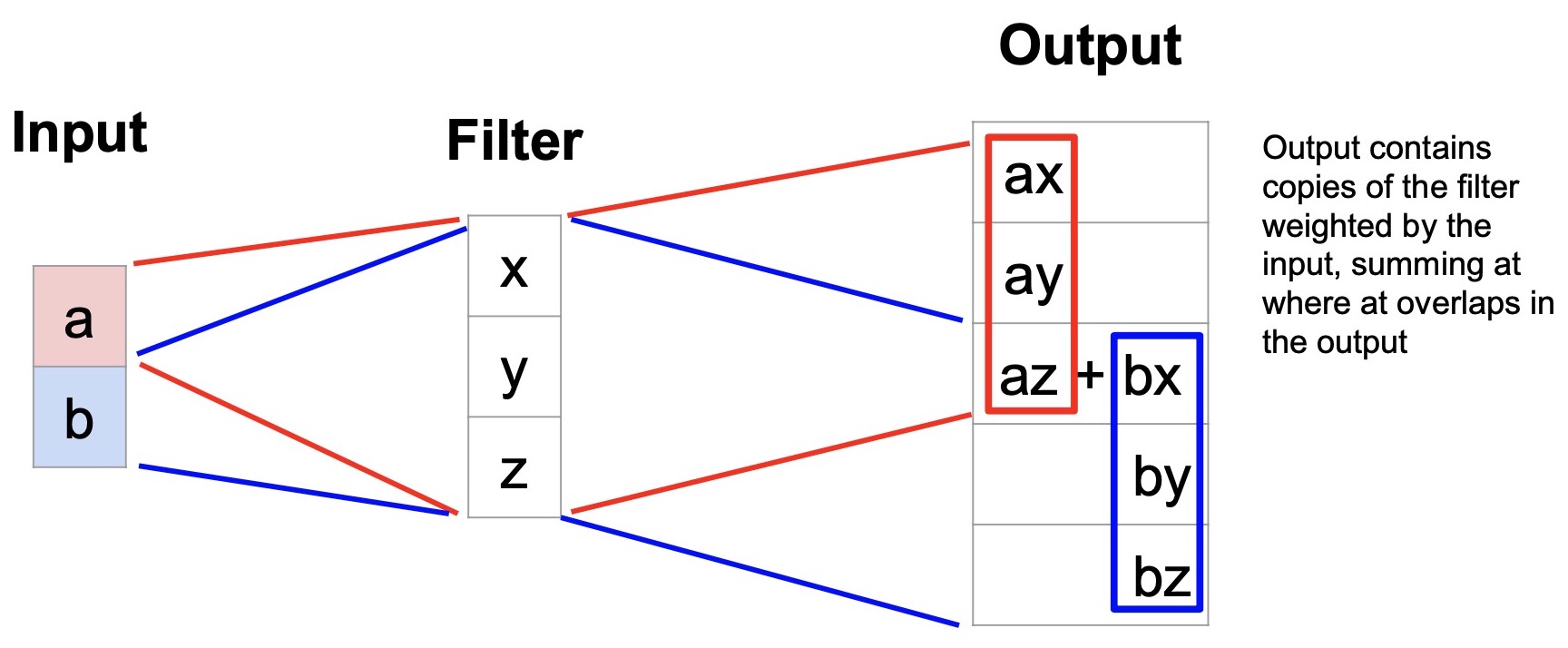
- Convolution as matrix multiplication:
- We can express a vanilla 1D convolution (and not ConvT) with a kernel size of 3, stride of 2, and padding of 1 as a matrix multiplication. In the diagram below, matrix \(X\) (composed of \(x\), \(y\) and \(z\) which are kernels) and vector \(a\) (which represents the input) are bound together by a convolution operation. Specifically, the first row of \(X\) performs a convolution with \(a\) and the second row of \(X\) performs an independent convolution again with \(a\). Note the padding in both \(x\) and \(a\). So vanilla convolutions can be expressed as matrix multiplication.
- On the other hand, the corresponding ConvT can be obtained by actually just taking the transpose of the weight (kernel/filter) matrix. So ConvT is equivalent to multiplying the transpose of the weight matrix with the input. This is essentially where the name transpose convolution comes from.
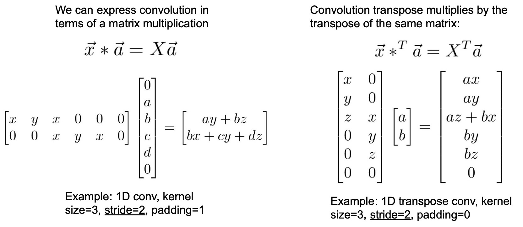
- The weight matrices in ConvT are thus learned similarly as in the case of vanilla convolutions, where these differ is how you “use” the matrices (transpose vs. no transpose).
-
Generalizing this to the 2D transpose convolution case, due to us performing summation in the overlapped regions, the values exhibit a stark increase in magnitude. This can lead to a checkerboard pattern where there are strides of values that are distinctly different than other values due to the summation. One way to fix this is to average out the values rather than doing a summation (but this won’t be the regular ConvT). Refer to chapter 4 in “A guide to convolution arithmetic for deep learning” by Dumoulin and Visin (2016) to learn about some ways to deal with this artifact of ConvT.
-
To summarize, for the semantic segmentation task, upsampling is accomplished using max unpooling or strided transpose convolutions. Actual implementations likely use a combination of the two. On the other hand, for downsampling, we utilize operators such as max pooling or strided convolutions to reduce the feature size and go deeper. We can train the model end-to-end with pixel-wise classification loss using backpropagation.
- Semantic segmentation has wide applications in vision such as autonomous driving, where you want to segment the road, obstacles and other moving objects, medical image segmentation to segment tumors from other regions etc.
- Turns out there is a critical limitation to the problem definition of semantic segmentation. Recall that semantic segmentation involves classifying/labeling each pixel in the image with a semantic category. But, what if we have two instances of the same object category in the same picture? With semantic segmentation, there is no way to distinguish between the pixels that belong to each of the objects. Consider the example of two “overlapping” cows in the same picture as shown in the figure below, wherein we have no way of telling which pixel belongs to which cow. This is an important limitation because a lot of the applications within vision require us to distinguish between different instances of the same category, for e.g., if we want to classify human poses with a segmentation mask, then we probably want to distinguish which pixels belong to which person.
- This is where the instance segmentation problem comes in. An instance segmentation model would be able to assign different labels to object instances even if they belong to the same category.
Before we talk about instance segmentation, let’s introduce the object detection problem first, since we’ll be building our instance segmentation on top of our object detection models.
Single Object Detection (Localization + Classification)
- The simplest formulation of object detection is called object localization where we assume there is only one object in the image and the model should learn to not only classify the object but also put a 2D bounding box around the object to indicate its location in the image. The bounding box is parameterized by 4 numbers: (i) \((X,\,Y,\,W,\,H)\) or (ii) \((X_1,\,Y_1,\,X_2,\,Y_2)\). In the first convention, \(X\) and \(Y\) specify the location of the top left corner of the box while the height and width specify the size of the box. In the second convention, \(X_1\) and \(Y_1\) specify the top left corner while \(X_2\) and \(Y_2\) specify the bottom right corner of the box. We will adopt the former convention for our discussion below.
- The simplest formulation for this problem as a learning approach is to treat the bounding box prediction as a regression problem, where we train a model to predict the 4 numbers with something like L2-loss.
- Here, we can take the object classification architecture taken before and add a separate output branch for doing regression in parallel to the classification output. This transforms an object localization and detection model a multi-task model because we’re telling the model to learn two tasks at the same time. Accordingly, we need to train the model with a mutli-task loss.
- A multi-task loss is a weighted sum of all the task-specific losses to balance the magnitude of the different loss terms. For e.g., we might want to multiply the classification loss and regression loss with different weighting factors to balance their contribution to the final multi-task loss. If the regression loss is say larger than the cross-entropy loss, we’d probably want to balance that, and these weights can serve as hyperparameters.
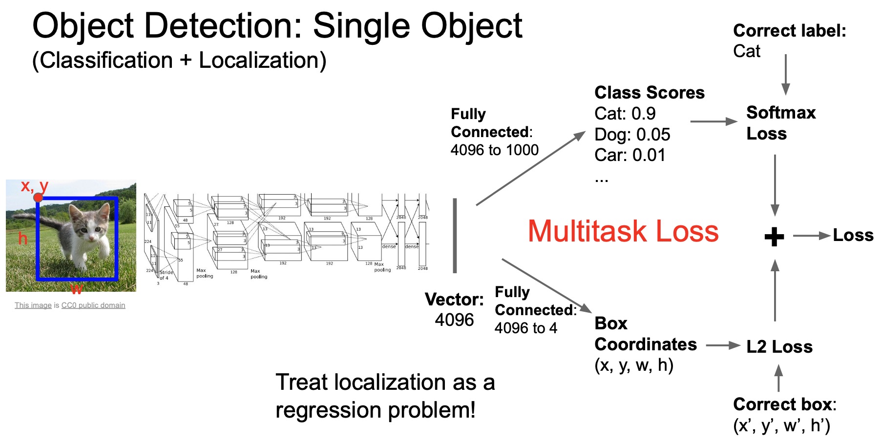
- So we train the network end-to-end with a label for classification and bounding box for localization. The only difference between object classification and detection is that instead of one classification output, we add another output for predicting the bounding box and train the two branches together.
- In summary,
- In this problem we want to classify the main object in the image and localize it using a bounding box.
- We assume there is one object in the image.
- We create a multi task network to accomplish the sub-tasks of classification and localization. The architecture is as following:
- Convolution network layers connected to:
- FC layers that classify the object (i.e., the vanilla object classification problem).
- FC layers that connects to four numbers: \((x,\,y,\,w,\,h)\)
- We treat localization as a regression problem.
- Convolution network layers connected to:
- Loss = SoftmaxLoss + L2 loss:
- Softmax loss for classification
- L2 loss for localization
- Often the first conv layers are pre-trained on a large image database (ImaegNet) such as AlexNet.
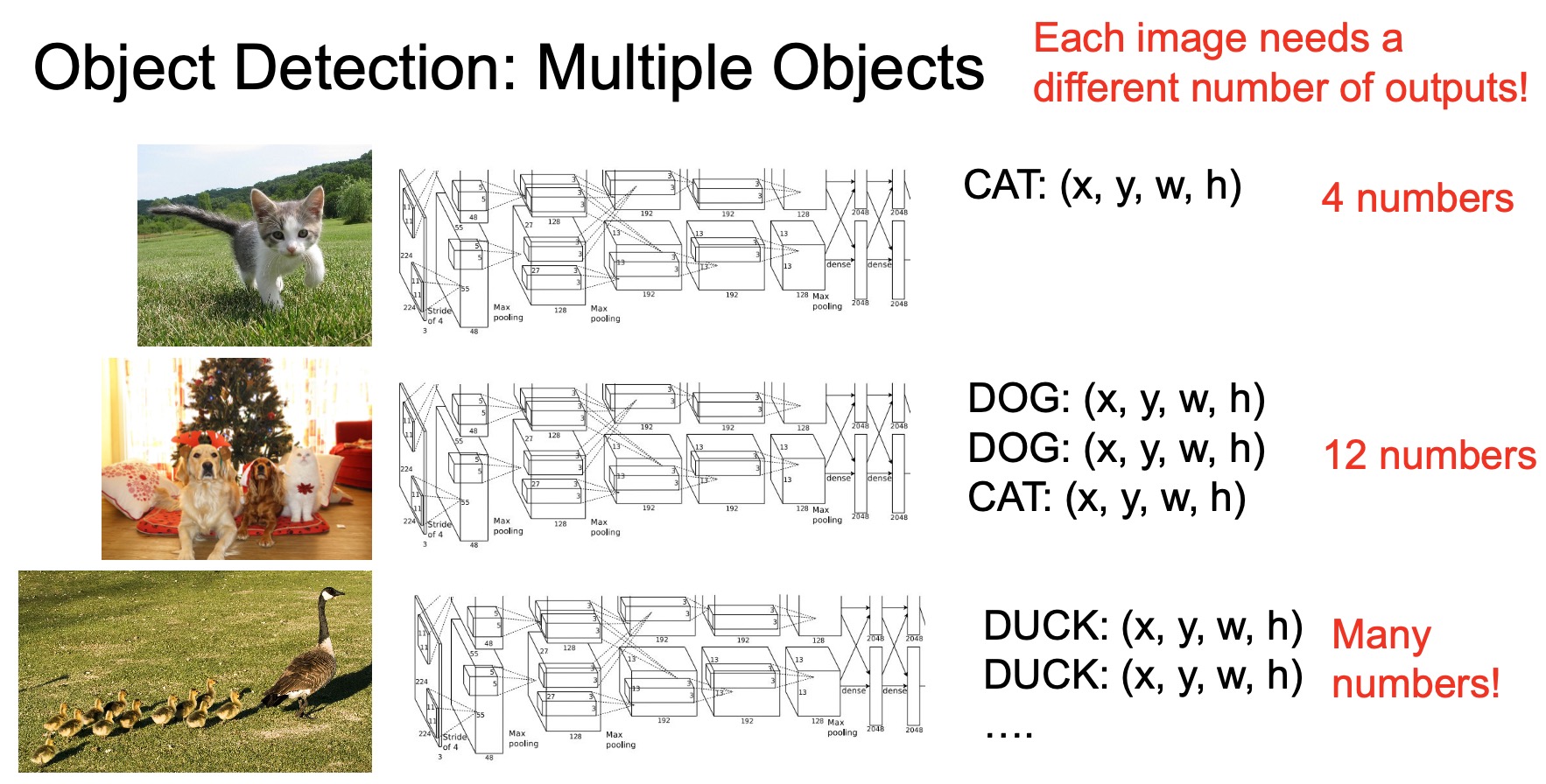
Multiple Object Detection
- Note that our strategy is still limited in its functionality in that it serves only the single-object case. When we talk about object detection, we’re usually talking about detecting multiple objects in the scene and we do not know the number of objects beforehand.
- In other words, the model needs to make predictions for different numbers of outputs for each image, as shown in the figure below. For e.g., here we see that different images require different number of (classification, bounding box) outputs. The architecture for single object detection localization we saw before would not be able to handle the multi-object detection case because it only outputs a single predicted class and four numbers for the bounding box co-ordinates. Thus the need arises for a different architecture.
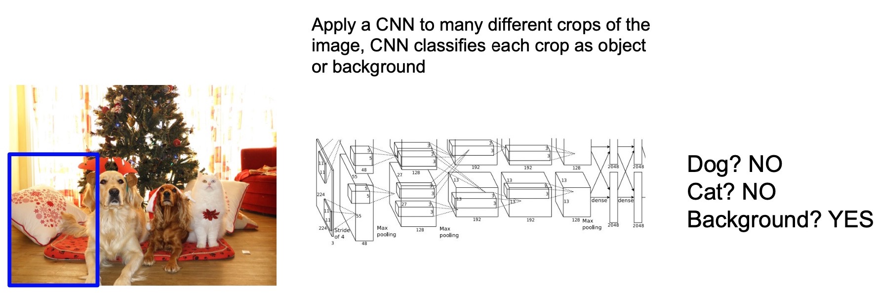
- So how do we design a model that can handle multiple objects? A possible strategy is to use a sliding window that goes over the image, similar to what we discussed for semantic segmentation. For each image crop we slide over, we can use an object classifier to figure out whether there is an object or not in the sliding window and the category of the object if one exists. For instance, assuming we’re trying to detect only dogs and cats (and their absence, which would simply be the background) in an image, for the sliding window position given below by the blue box, since there is no dog or cat in the image crop given by the box, the model outputs the background class indicating that there are no valid objects present in the bounding box.
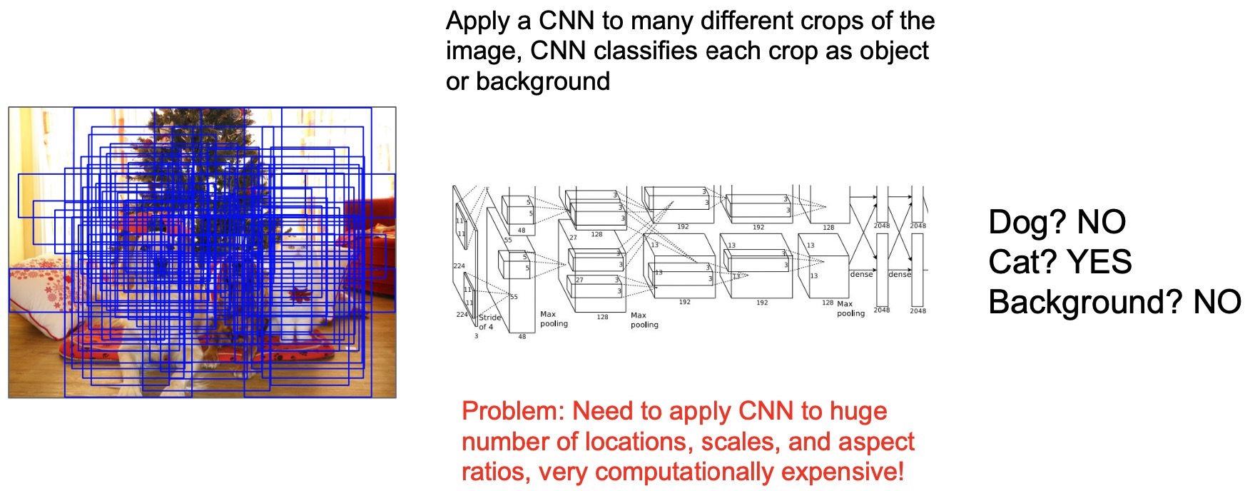
- Under this approach, we slide this window over the entire image. In summary, this approach combines the concept of a sliding window with classification and enables (i) predicting variable number of objects in each image and, (ii) outputting both the object category and directly using the parameters for the sliding window as a 2D bounding box prediction output.
- But there is a problem with this approach, very similar to what we had for the sliding window approach for semantic segmentation. It’s the same issue of computation efficiency, but this time only a lot worse. So the main issue is that the sliding window not only needs to go to go over different locations in the image but also has to consider different sizes of the objects, as shown in the figure below. For e.g., dogs and cats are of different sizes and even the same object can also appear differently depending on the distance to the camera. So we need to vary the scale of the sliding window to cover all possible objects.
- We would need to vary the aspect ratios of boxes to accurately detect things like say, lamp-posts, which require very thin boxes. Unfortunately, this creates a combinatorial search space of both the location and the box sizes. This becomes very expensive to go through even for a single image.
Region Proposals: Selective Search
- So the question then is how can we capture all of the objects without having to go through all possible boxes?
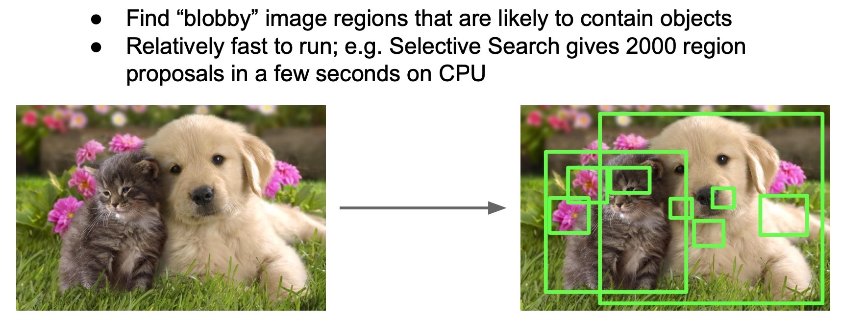
- Selecting windows that are likely to contain objects is known as the region proposal problem (shown in the figure below).
- A very effective approach for this problem is a classic computer vision technique called selective search, which is an efficient way to select regions that are likely to contain objects and we can run our expensive neural net classifier on top of these selected regions to save compute. The typical region selection algorithms rely on hand-crafted functions such as looking for things that look like objects (based on a sliding window approach that looks for color, texture, size and shape similarity). For instance, we can use prevalent computer vision techniques such as blob detectors to find regions that contain blob-like structures because these regions are more likely to contain objects as opposed to uniform regions which are unlikely to contain objects.
- We can then run our neural net classifier on top of these blobby areas to do a more accurate classification. And often cases, we can reduce the number of classifier runs from of the order of millions to the order of thousands.
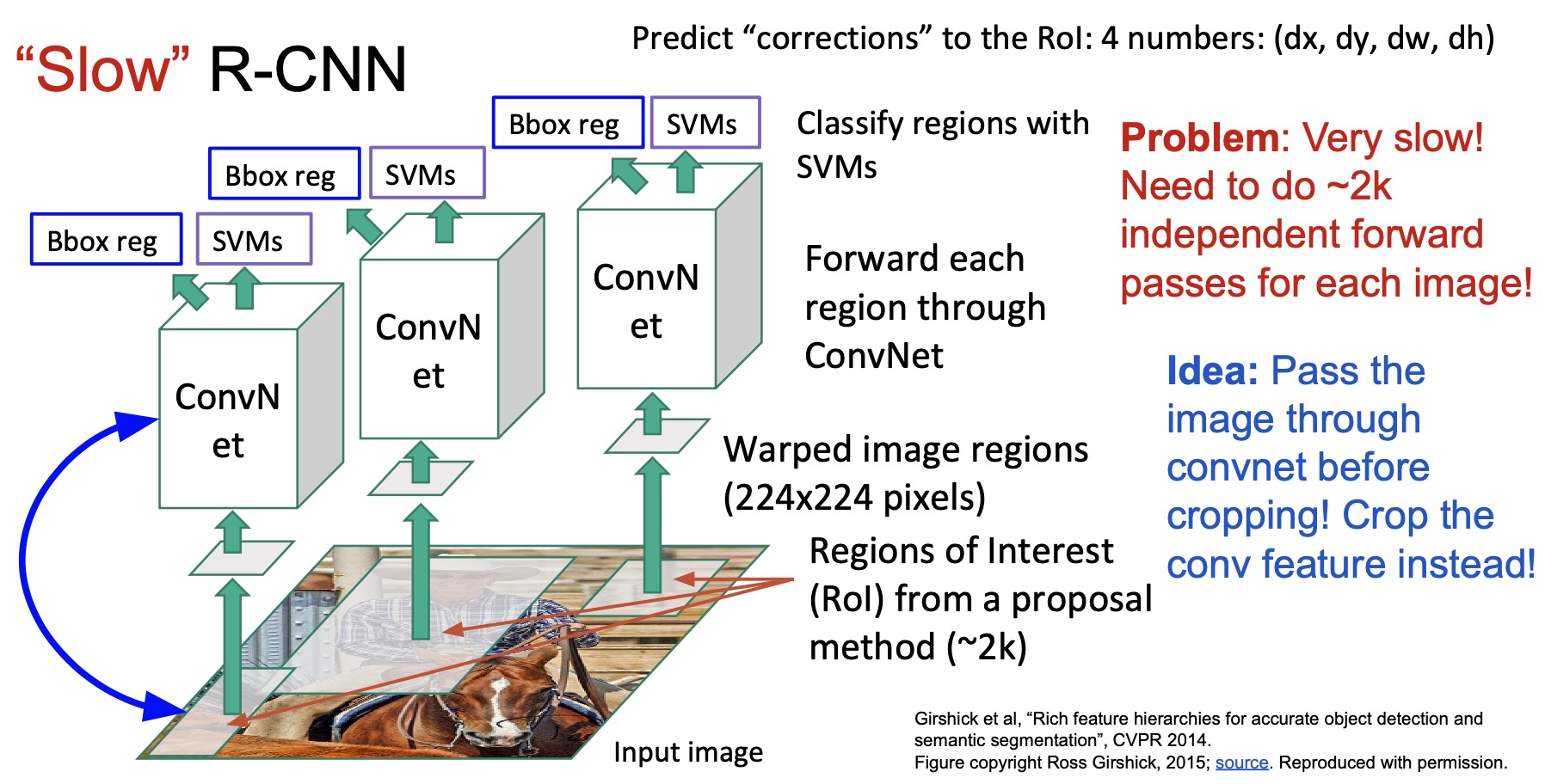
R-CNN
- The first paper that puts all of these ideas together is the R-CNN paper “Rich feature hierarchies for accurate object detection and semantic segmentation” (2013) by Girschick.
- As the first step, R-CNN used selective search to find Regions of Interest (RoIs) that are likely to contain objects. This step generates of the order of a couple of thousand regions. Note that since we do not actually care about the object category yet, the region selection step is category agnostic, which implies that we need a classification layer next.
- R-CNN then resizes these RoIs into image crops of the same size (R-CNN re-sized them to \(224 \times 224\) pixels), because these regions are initially of different sizes. They need to be resized to the same size to perform the next step which is passing them through a ConvNet pretrained on ImageNet (the original R-CNN paper used a pre-trained AlexNet, which is the first ConvNet-based winner on the ImageNet challenge). The region why these image crops/RoIs were resized to \(224 \times 224\) pixels is because that’s the original size that AlexNet was trained on. These uniformly (re-)sized RoIs were called “warped” image regions.
- Finally, they use Support Vector Machines (SVMs) trained on the features of the last layer of the pre-trained ConvNet to classify the regions so they did not train everything end-to-end, infact they just trained a linear classifier with SVM loss on top of that.
- Remember that back then, it was very expensive to train models end-to-end, especially a compute-intensive task like object detection, which is why they opted for a less expensive solution.
- They also trained a linear regression model to refine the RoI locations. Recall that these regions are generated by selective search and the generated boxes may not perfectly align with the actual object boundary, so they trained this extra output to make the bounding box locations more accurate. As an intuitive example of bounding-box regression, consider a case where the region proposal found a cat but if the bounding box does not contain its tail, a regression-based model should be able to train the model to learn that cats have a tail and modify the original proposals based on the input by making the bounding box wider and capturing the tail.
- There are are many problems with this approach such as:
- Not trainable end-to-end (only the top layers are trainable as a group)
- The use of a separate linear classifier (SVM) for classification
- The questionable image-resize to align with AlexNet input size
- However, the most important thing is this was a seminal paper that laid the foundations for modern deep-learning object detection architectures. A lot of the ideas proposed herein (seen in the figure below), such as:
- Utilizing a two-stage algorithm to perform object detection: (i) doing region proposals and suggesting bounding boxes, and (ii) refining aforementioned bounding boxes and classifying regions into semantic classes,
- Resizing RoIs (or feature maps, as we shall see in Fast R-CNN), and
- Using a “backbone” ConvNet for feature generation.
- … are still being used in almost all current deep learning-based 2D object detection models, which basically propose improved versions of these ideas.
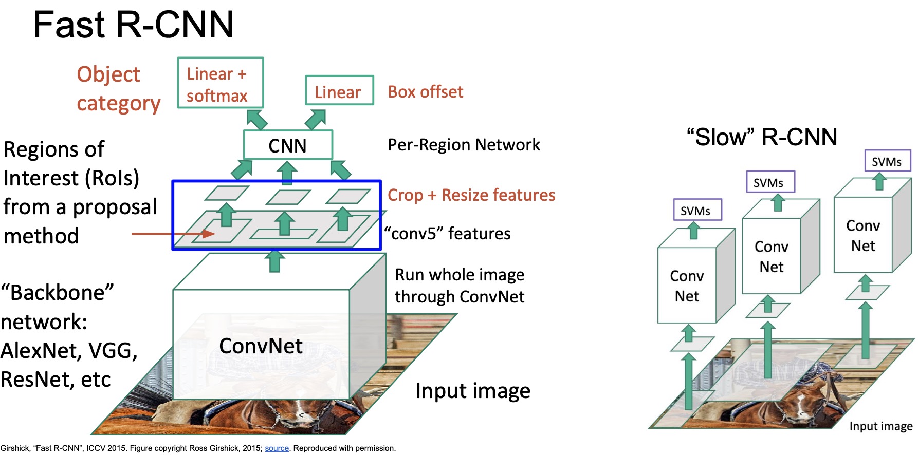
Fast R-CNN
- The first problem with R-CNN is that it is very slow. Although we have reduced the number of possible regions from millions to thousands, we still need to pass each region proposal through the ConvNet (AlexNet, in case of R-CNN) thousands of times in order to process each image and that’s very expensive.
- A possible solution is that instead of cropping and resizing the image and then passing them through the ConvNet, we can pass the entire image through the ConvNet first and then crop and resize the Conv features associated with the region proposals instead. This would avoid us having to pass through the expensive Conv layers thousands of times to process a single image.
- This is exactly the idea behind “Fast R-CNN” (2015) proposed by Girshick, a faster version of the original R-CNN.
- Given the same input image, we can pass the entire image through a ConvNet “backbone” (without the FC layers). A Backbone network can be a network that can serve as an image feature extractor (trained on a large labelled image database such as ImageNet) such as AlexNet, VGG, ResNet etc. In this paper, they used the Conv blocks of VGG-Net (by truncating the FC layers and only using the conv layers) and extract the feature maps after the Conv-5 block.
- Next, instead of cropping the image, they directly crop the Conv-5 feature map. The cropped features are then similarly resized (as in R-CNN) and passed through a shallower per-region network to generate object categories and the bounding boxes correction values for each region.
- The Fast R-CNN architecture can be trained end-to-end. Even though there are still several resizing and cropping steps, note that the cropping and resizing is done directly on the feature map and not on the image.
- Digging deeper into the Fast R-CNN architecture:
- Backbone network: ConvNet architecture trained a large labelled image database such as ImageNet, such as AlexNet, VGG, ResNet etc.
- Per-region network: Very shallow ConvNet with some linear layers that process each feature crop individually.
- The next question is… what is this feature cropping and resizing operation? How do we crop a Conv activation map if it is not even of the same size as the original image? Is the process of cropping and resizing the features even differentiable? Enter Region of Interest Pooling!
Region of Interest (RoI) Pooling
- The cropping and resizing operation is known as RoI pooling. The goal of RoI pooling is to extract features from an activation map given a region and reduce the new feature map to a fixed size tensor for the downstream layers to process.
- First, we’ll extract the convolutional feature map of the entire image using the Conv backbone. Let’s say that this yields a feature map of size \(512 \times 20 \times 15\) given the original image of \(3 \times 640 \times 480\). Note the channel-first convention being followed here, where \(512\) is feature-dimension channel size, and \(20 \times 15\) is the spatial dimension size.
- In the figure below, the green box highlights the region proposal. Our goal is to use the same region but crop it out from the feature map.
- First, because the Conv backbone downsamples the image from \(640 \times 480\) to \(20 \times 15\), we have to scale down the region accordingly to perform cropping on the feature map.
- Because of the downsampling, the region in the feature space may not directly align with the regions of pixels. In other words, the border of the region may be in between two pixels, which implies that regions may contain partial pixels. So how do we do this cropping?
- The RoI pooling operation is to first snap the region to as close as the approximate spatial feature location. So we’re basically just rounding the sub-pixel locations of region bounding boxes to integers. Note that this is a heuristic and can introduce a lot of noise, especially if the region is very small. We’ll talk about how to improve it later.
- Recall that our goal is to resize a region of arbitrary size (after cropping) to a fixed size tensor and that this resizing operation has to be differentiable. Now that we have this region that we can directly crop because it lines with a region of whole pixels, the question arises… how do we do the resizing? how do we make the resizing differentiable?
- Let’s say that we want to resize this cropped feature from \(512 \times 20 \times 15\) (shown by the blue region in the figure below) to a tensor of size \(512 \times 2 \times 2\). How do we do this?
- What RoI pooling does is it first divides the region into a \(2 \times 2\) grid of roughly equal sub-regions as shown in the figure below.
- How the division is done is specific to the implementation but the number of grids we want to divide into should be equal to the final size of the tensor we’re looking for.
- Next, we use max pooling to reduce the spatial size of the tensor to \(2 \times 2\) so each sub-region gets reduced to a single pixel so the output tensor becomes \(512 \times 2 \times 2\).
- In practice, we might want to do max pooling and to a \(7 \times 7\) region instead of a \(2 \times 2\) region (the figure below shows a \(2 \times 2\) region for simplicity).
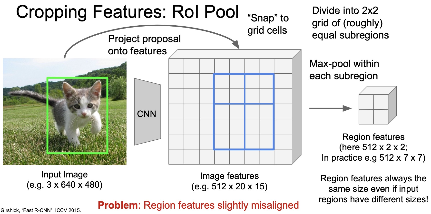
- Overall, the goal of RoI pooling is to reduce the resize a region of arbitrary size (after cropping) to a tensor of specific size, for e.g., \(2 \times 2\) or \(7 \times 7\).
- RoI pooling has to handle a lot of corner cases. For e.g., what if the region is smaller than the target size?
- For e.g., it is not very straightforward to resize a region of size \(5 \times 4\) to \(7 \times 7\) – in this case, you’re actually scaling up the feature! So there needs to be lot of heuristics in implementing these RoI pooling layers.
- Also, note that since Girshick proposed “Fast R-CNN” in 2015, the authors had to implement both the forward and backward pass of RoI pooling using CUDA, which makes it notoriously hard to get all the intricate steps right!
- All of these corner cases will cause the region features to be slight misaligned with features corresponding to the actual image region. So the question is… is there a better way to handle all of these corner cases more gracefully and in a more principled way without these heuristics? Here is where RoI align comes in!
Performance comparison between R-CNN vs. Fast R-CNN
- Recall that Fast R-CNN used the shared convolutional backbone to make the image processing a lot more efficient. So how do they compare in terms of runtime speed?
- In training, Fast R-CNN is roughly \(10x\) faster than R-CNN. Testing time is \(>20x\) faster.
- But, if we take a closer look at the breakdown comparing the Fast R-CNN with and without the region proposal steps (“selective search”), we see that the main bottleneck is Fast R-CNN is actually computing the region proposals using selective search. So the entire operation takes \(2.3\) seconds which is split as \(~2\) seconds for region proposal and \(0.32\) seconds to classify the object after obtaining region proposals. The runtime, thus, is dominated by region proposals.
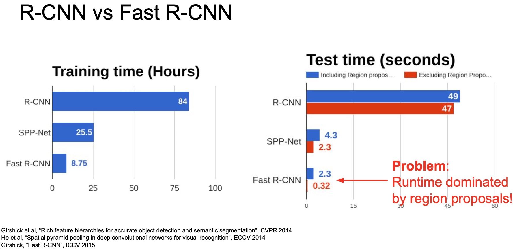
- So the question then is… how do we make this region proposal step faster? Enter Faster R-CNN.
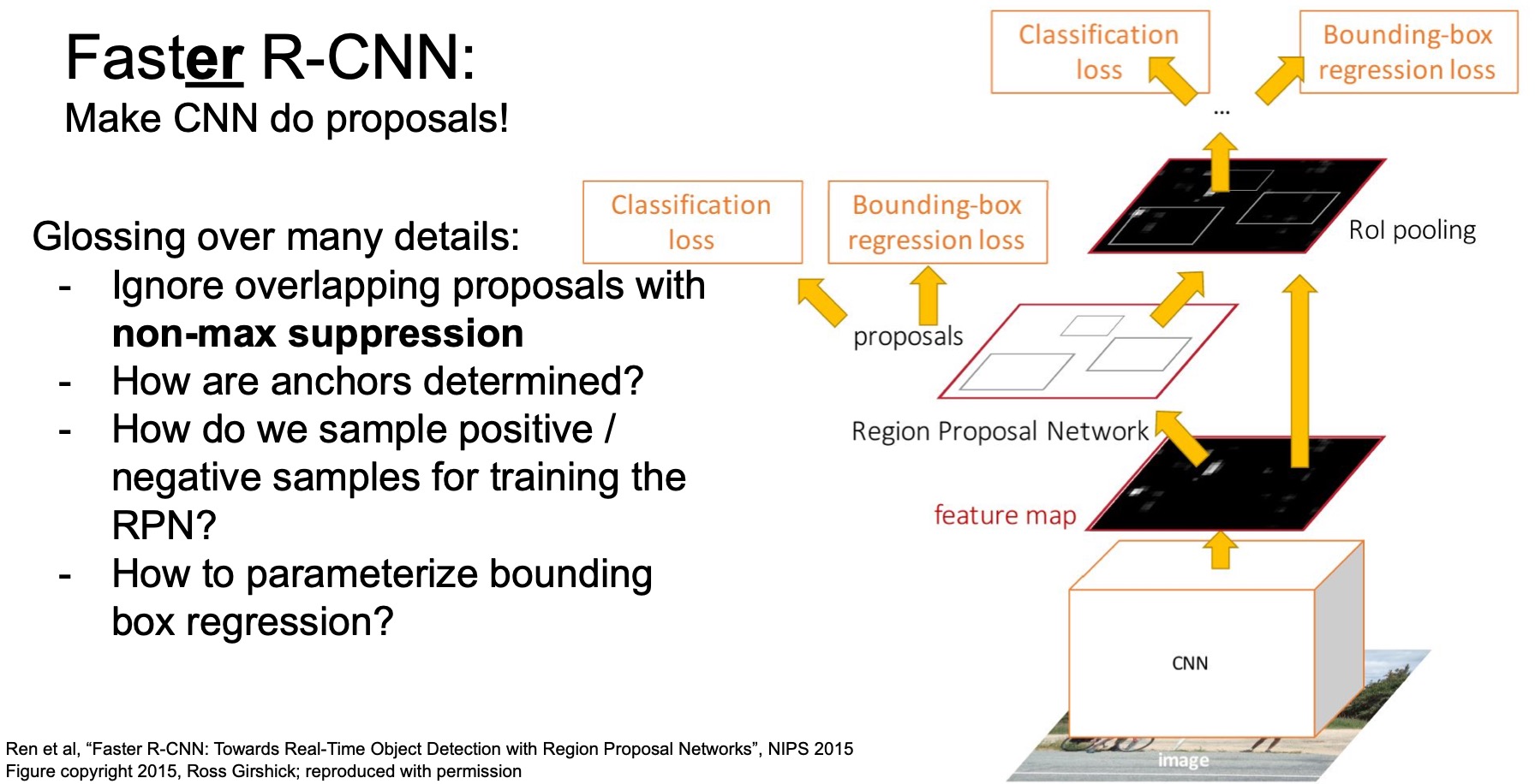
Faster R-CNN
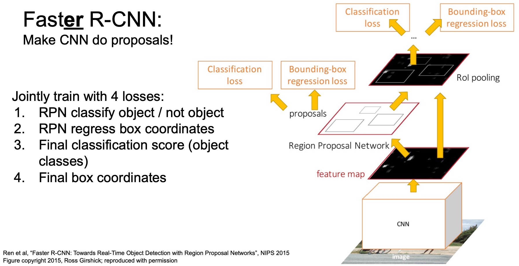
- Follow-up to Fast R-CNN, proposed by Ren et al. as “Faster R-CNN: Towards Real-Time Object Detection with Region Proposal Networks” (2015).
- Faster R-CNN tries to make the region proposal part faster. Instead of relying on an external selective search algorithm, the network now has a built-in Region Proposal Network (RPN) that actually uses the convolutional features to decide whether an object exists in a given region or not and generate the region proposals inside the network.
- So what exactly does this region proposal network do? Let’s take an example of image encoded using a \(512 \times 20 \times 15\) feature map.
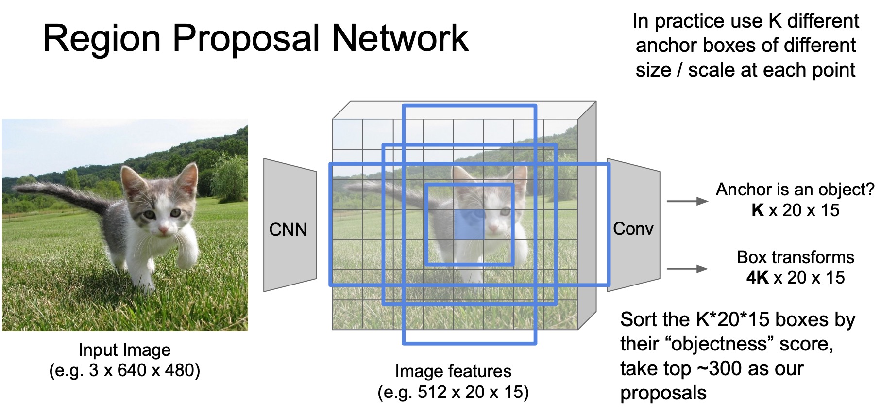
- The first step of RPN is to specify a set of anchor boxes. These anchor boxes are essentially regions sampled at different location/size/aspect ratio, similar to the sliding window.
- Note that anchors are different than sliding windows, in the sense that these anchors are sampled relatively sparsely as opposed to the multitude of sliding windows used in previous R-CNN/Fast R-CNN architectures. The original paper just used 2000 anchor boxes, which is a lot less than the number of sliding window instances as shown in the figure below.
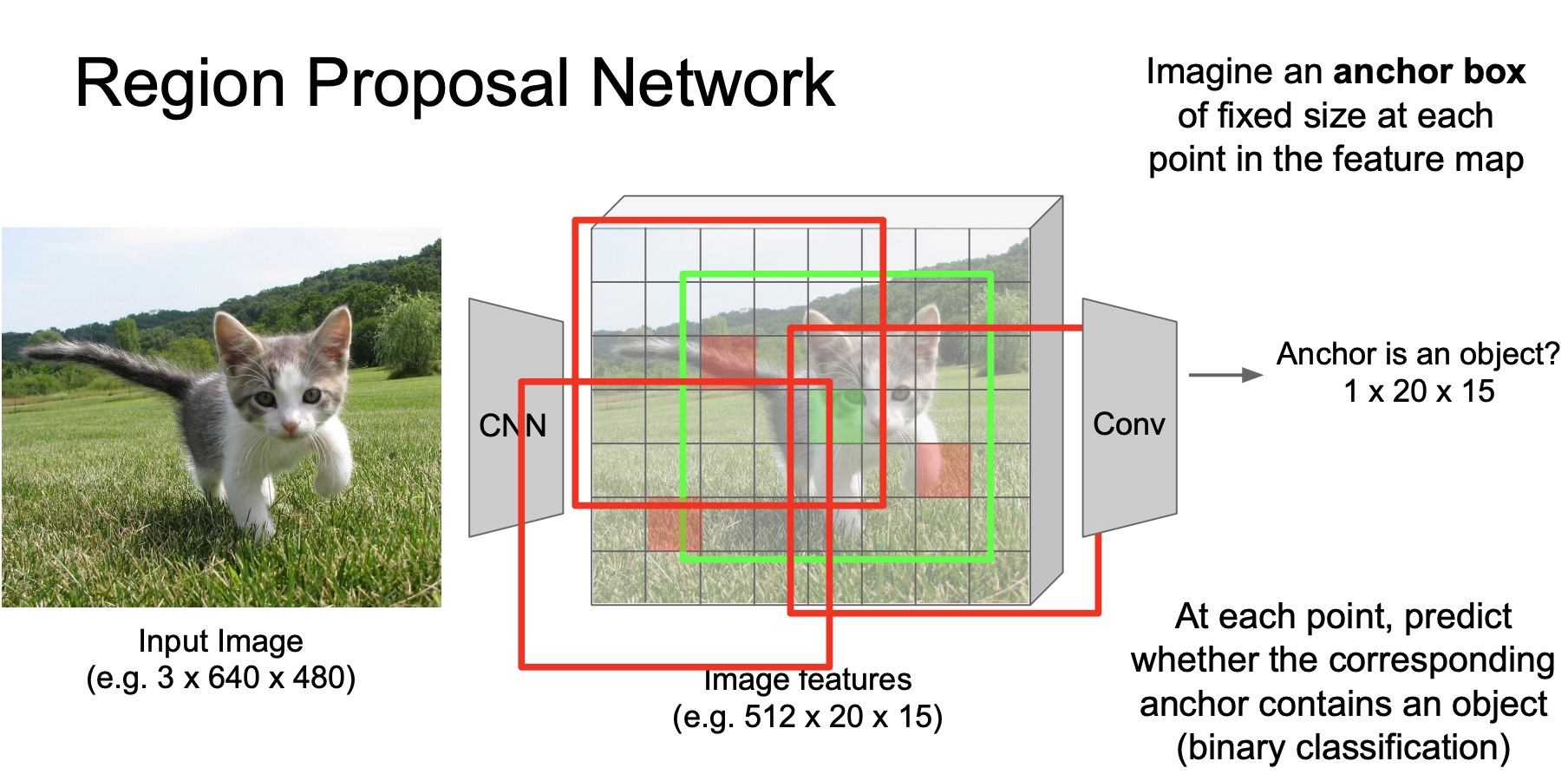
- These anchors only cover the region where objects usually occur in natural images and they use the same set of anchors for every input image. In some sense, you can consider these anchors just as an input to the network – sort of a prior about where objects usually occur. Note that anchor boxes being this sparse are in no way good enough to serve as a region proposal mechanism yet.
- What RPN does is that they pass the features at the centers of these regions through a very shallow ConvNet that predicts whether there is an object in the anchor box (centered at this region). Essentially, we are making a prediction w.r.t. each of the anchor boxes using the conv features by deciding whether there is an object around this center pixel or not. Remember that at this stage, each conv feature has a large receptive field so it essentially is looking at a large are of pixels around the center pixel w.r.t. the input image.
Each point in the feature map (shown in the figure below) is responsible for detecting an object in the anchor box centered at that point.
- For the anchors that are determined to be positive, which means they are likely to contain objects, we also predict the corrections that should be applied to the anchor to better align with the ground truth, because these anchors are chosen apriori and may not align with the objects in the anchor as-is. This is called the process of anchor box correction – same as what R-CNN follows for bounding box correction. The correction objective is again, usually trained with a regression loss.
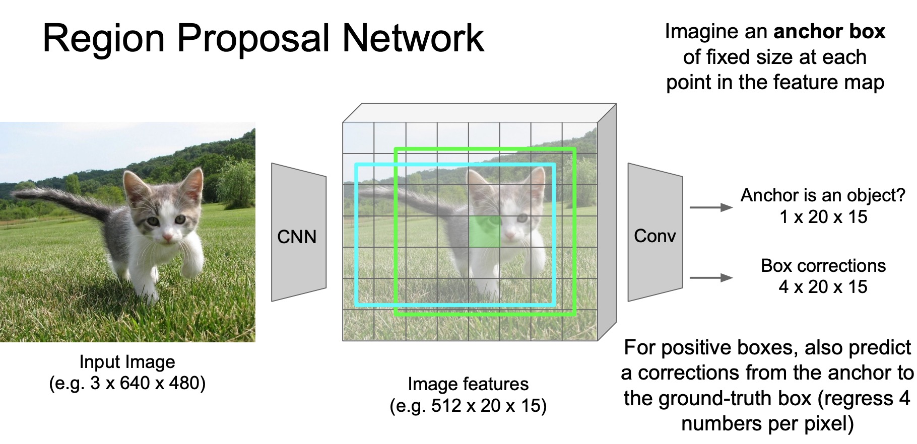
- Another question is… How do we generate this ground truth for training RPN? how do we craft our binary classification + regression objective?
- According to the paper, an anchor is labelled positive if it intersects with the nearest ground truth object bounding box with an overlap of \(>0.5\), which is a hyperparameter. In terms of binary classification labels, this means a label of 1 if the overlap is \(>0.5\), else 0.
- Given \(K\) anchors, the RPN outputs \(K\) classification predictions and \(4K\) regression predictions, basically predicting \(K \times 20 \times 15\) numbers for classification and \(4K \times 20 \times 15\) for anchor box regression predictions (where \(20 \times 15\) are the spatial dimensions of the image).
- Finally, these boxes are sorted by their binary classification score, which the paper calls an objectiveness score. The top \(300\) boxes are taken as region proposals for the next step.
- Two-stage bounding box correction:
- The rest of the model is the same as Fast R-CNN, including the RoI pooling layer, final classification and bounding box correction loss so each bounding box actually goes through two rounds of spatial location correction. The first is inside the RPN and the second is at the final output stage. So the bounding box predictions from Faster R-CNN are usually very accurate because of two-stage correction.
- In total, Faster R-CNN has 4 training losses: 2 losses for RPN and 2 losses for the final output. Jointly training these four losses is not easy and requires a fair amount of hyperparameter tuning to get the best performance.
Suppressing overlapping predictions
- Non-max suppression (NMS) is a common technique in object detection that helps judiciously pick the right proposal region in case of overlapping proposals. NMS processes the output from the network to filter out the boxes that have too much overlap because they mostly likely correspond to the same object.
- Training RPN requires sampling background boxes for the binary classification loss but how many boxes do we sample? how do we balance the loss from the negative samples and positive samples? how do we parameterize the bounding box regression?
- Read the paper to find more!
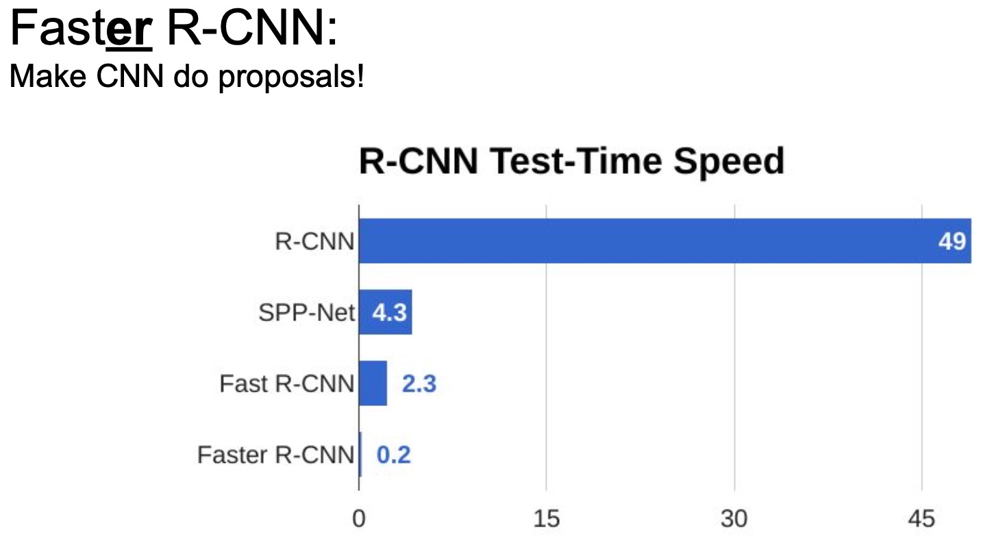
Performance comparison of Faster R-CNN vs. Fast R-CNN vs. R-CNN
- In terms of computation efficiency, Faster R-CNN can process an image in just \(0.2\) seconds and is \(10x\) faster than Fast R-CNN and 2 orders of magnitude faster than the original R-CNN. Quite a leap in terms of computation speed!
Region of Interest (RoI) Align
- Proposed by He et al. in “Mask R-CNN” (2017) as the successor to RoI pooling. RoI align is an upgrade to RoI pooling with the ability to handle all the corner cases we discussed above in a more principled way.
- So the first question RoI align tries is to answer is that can we do cropping and resizing without snapping the region to the nearest grid location? what’s a better way to accomplish this? The answer is yes, we can! Instead of snapping, diving the grid into \(2 \times 2\) equal sub-regions (again), but now they are equal sub-regions and not roughly equal sub-regions.
- Next, sample features based on fixed stride of grid locations in each sub-region (indicated by the green dots in the figure below). In other words, we take samples that are evenly spaced inside these sub-regions to extract features. These green dots are thus the locations we want to extract features from using the base feature activation map.
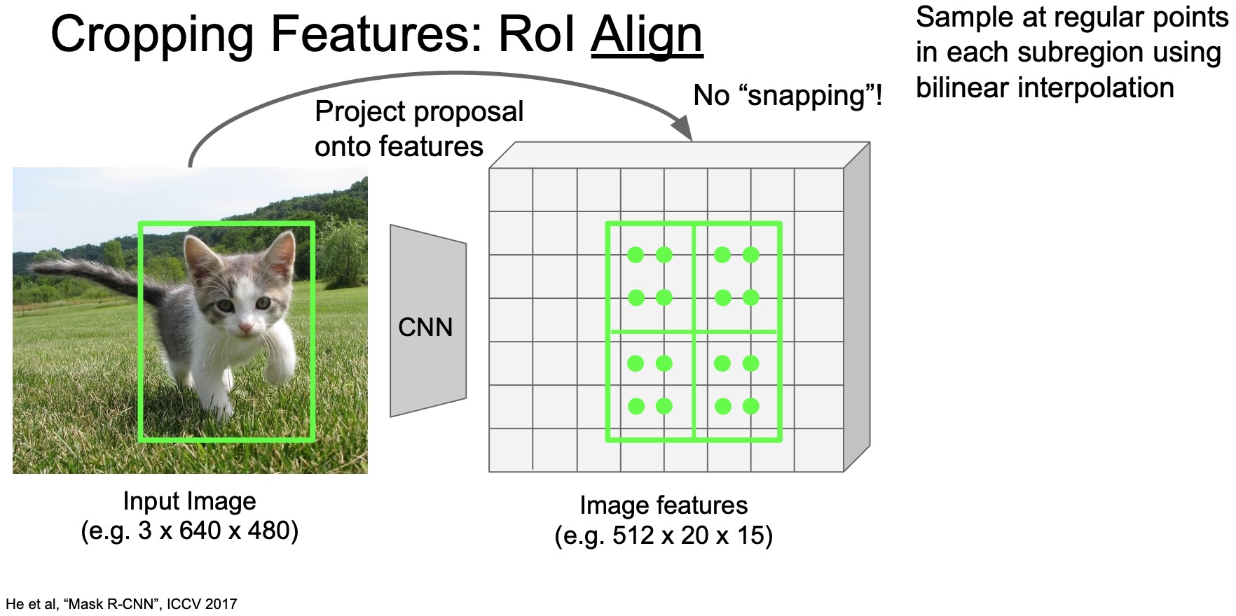
- But the original problem still persists, i.e., we can’t extract features at locations that are not exactly aligned with whole pixels. In other words, we still need to deal with extracting features from in between pixels.
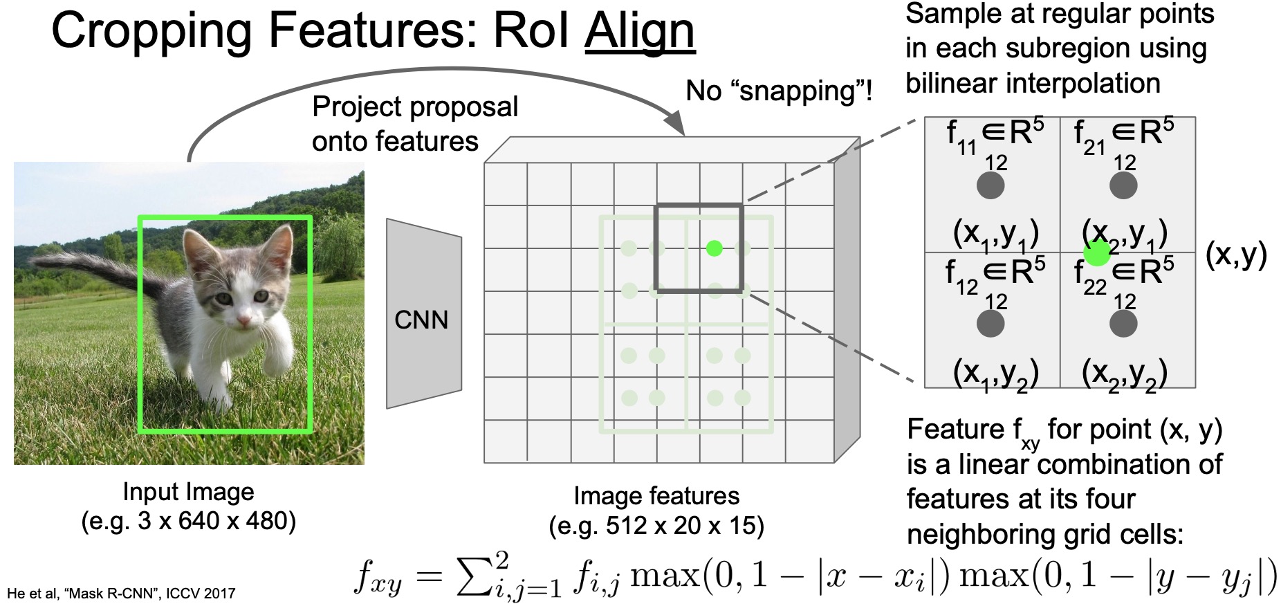
- What RoI align does is that it extracts features from these “in-between” locations using a technique called as bilinear interpolation.
- Here’s how bilinear interpolation works. For a location where we want to extract features from (say, the green dot in the figure below), instead of say taking the features from the nearest pixel, we take a linear combination of the four nearest feature pixels. The combination weight is determined by the distance from the target location to each of the four neighboring feature pixels.
- Say your grid point is at location \((x, y)\), then you want to find neighbors \((x_i, y_j)\) where \(i\), \(j\) are either 1 or 2. Use the relative distance from \((x, y)\) to weigh how much each of the neighboring feature pixels will contribute to the final representation.
- The feature extraction process (“bilinear interpolation”) can be expressed using the equation at the bottom of the image below.
- Notice that this is just a summation over two max terms and all of these operations are differentiable, including the max operator.
- So now we are able to extract features even if the grid is sampled in between two pixels. Once we have the features at each grid location, we can again take a maxpool of each sub-region and reduce it to the desired size depending on how many sub-regions we define, as shown in the figure below.

- Because we’re free to choose this grid resolution, you can resize region features to any target tensor size we like. Note that with this being the principled way to handle the feature extraction process, there’s no corner cases anymore.
- RoI align improves object detection performance quite a lot compared to RoI pooling.
One stage vs. two stage object detector
- Faster R-CNN is a two stage object detector where the first stage featurizes the images and generates the initial batch of region proposals. The second stage is to process each proposal individually to classify and refine these regions and thus yield the final prediction.
- The question then is… do we really need the second stage? why can’t we just add the object classification loss to the first stage and call it our new output?
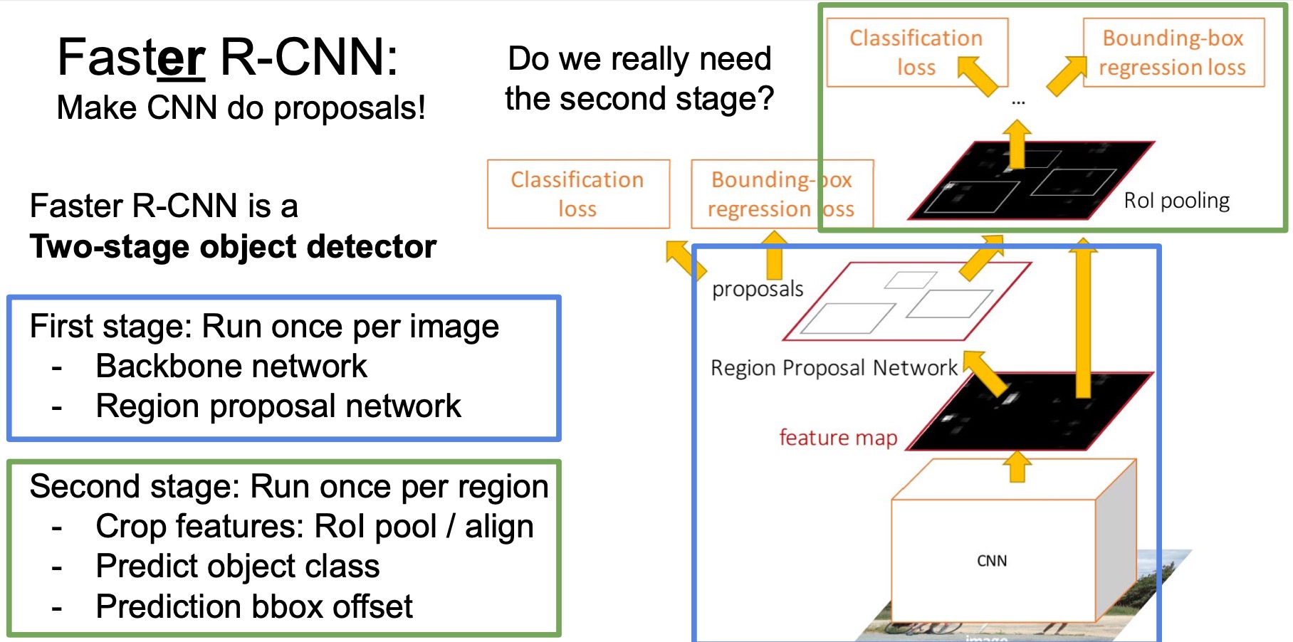
- A parallel thread of work on single stage object detectors follows this idea.
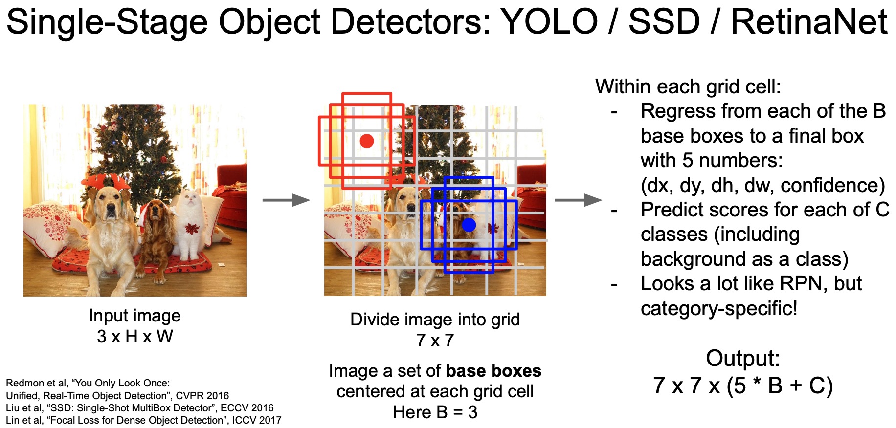
You Only Look Once (YOLO)
- You Only Look Once (YOLO) is a popular single-stage object detector that basically divides the input image into a grid. For each grill cell, it utilizes a bunch of “base boxes” (what Faster R-CNN calls “anchor boxes”) and outputs the bounding box corrections for each base box. It also predicts the class for each cell and uses that as the class predictions for the predicted boxes.
- YOLO outputs all the bounding boxes and their classes all at once in a single forward pass so there’s no second stage. Hence called the single-stage detector.
- Some other works in this line of research such as SSD and RetinaNet.
- Key takeaways
- Faster R-CNN is slower but more accurate.
- SSD/YOLO is much faster but not as accurate.
Object Detection: Summary
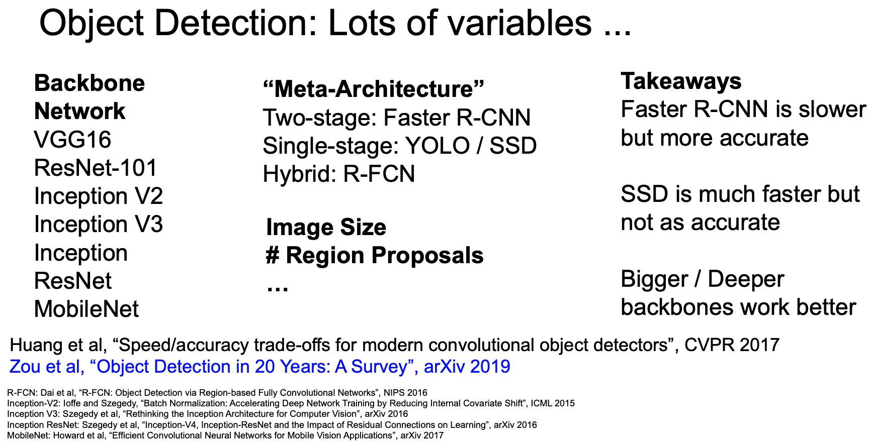
- There are different types of “meta” object detection architectures. Single-stage detectors such as YOLO are known to be less accurate but a lot faster than two-stage detectors such as Faster R-CNN. So the single stage detectors are often used to deploy in limited-compute settings such as mobile devices.
- Other variables that might affect the accuracy and computational efficiency of the model:
- Backbone network: VGG-16/19, ResNet-50/101, Inception V1/V2/V3, MobileNet.
- Number of region proposals: 300 (Faster R-CNN).
- 2D object detection is potentially the most important task in modern computer vision in the domain of scene understanding in computer vision.
- To get a holistic view of the field of 2D objection: “Object Detection in 20 Years: A Survey” (2019) by Zuo et al.
Instance Segmentation
- This is one of the toughest and relevant problems in the field of computer vision as of now.
- Not only want to predict categories of each pixel but also want to tell which object instance does each pixel belong to (shown below).
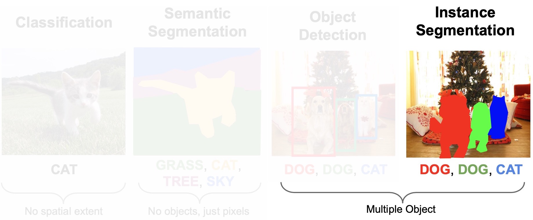
- Our goal is to build an instance segmentation model on top of the object detection architecture. What we essentially want to do is semantic segmentation inside each predicted bounding box. Each bounding box essentially corresponds to a single object instance and if we just do semantic segmentation inside the box, we’re basically doing instance segmentation.
Semantic segmentation inside each bounding box = Instance segmentation.
- The most straightforward way is to add a semantic segmentation architecture as part of the Faster R-CNN network, which is basically what “Mask R-CNN” (2017) does.

- Concretely, what Mask R-CNN does is that it adds this mini semantic segmentation network and runs this network on top of each region proposal. Mask R-CNN utilizes an RoI align layer that encodes region features into a fixed size tensor and this mini semantic segmentation network is essentially a fully convolutional network that scales the spatial dimensions upto a higher resolution semantic segmentation map through a series of convolutions and upsampling layers.
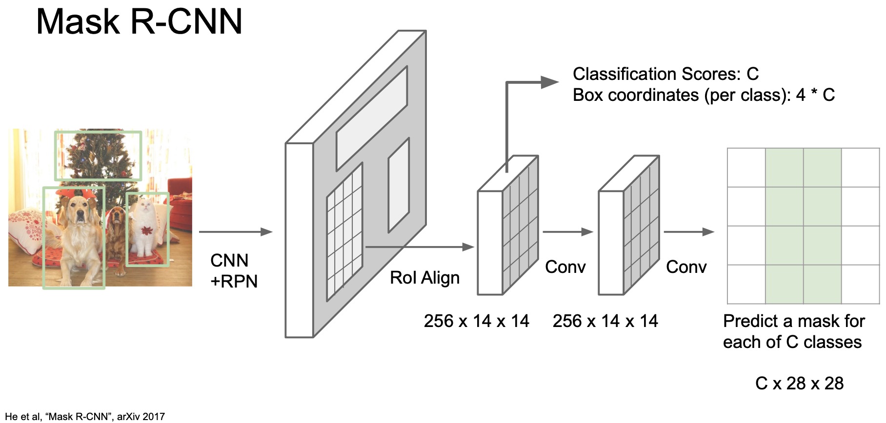
- We can train this network end-to-end with a ground truth segmentation mask. Mask R-CNN is essentially thus a very small semantic segmentation network on top of a region proposal network.
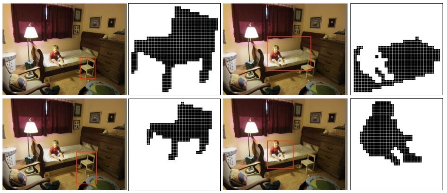
- To give a sense of what the output of Mask R-CNN looks like:
- Given an input image and the region proposals, we can see that the network not only detects the bounding box, but also segments the chair from the background (top left).
- For different region proposals, it outputs different masks accordingly (bottom left).
- Given the same region, it can segment other objects within that region (top/bottom right).
- The figure below shows an example of some mask training targets and Mask R-CNN’s instance mask extraction capabilities.
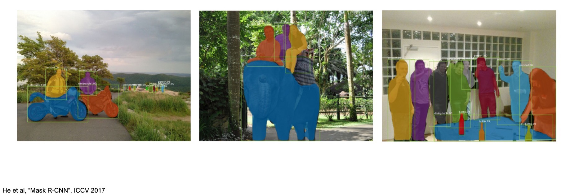
- If we train Mask R-CNN on the MS COCO object instance segmentation dataset, we can see that it not only can do object detection, it can also segment pixels that belong to the object instance so effectively we have achieved instance segmentation. Empirically, the performance is really good especially on common categories such as humans, objects etc.
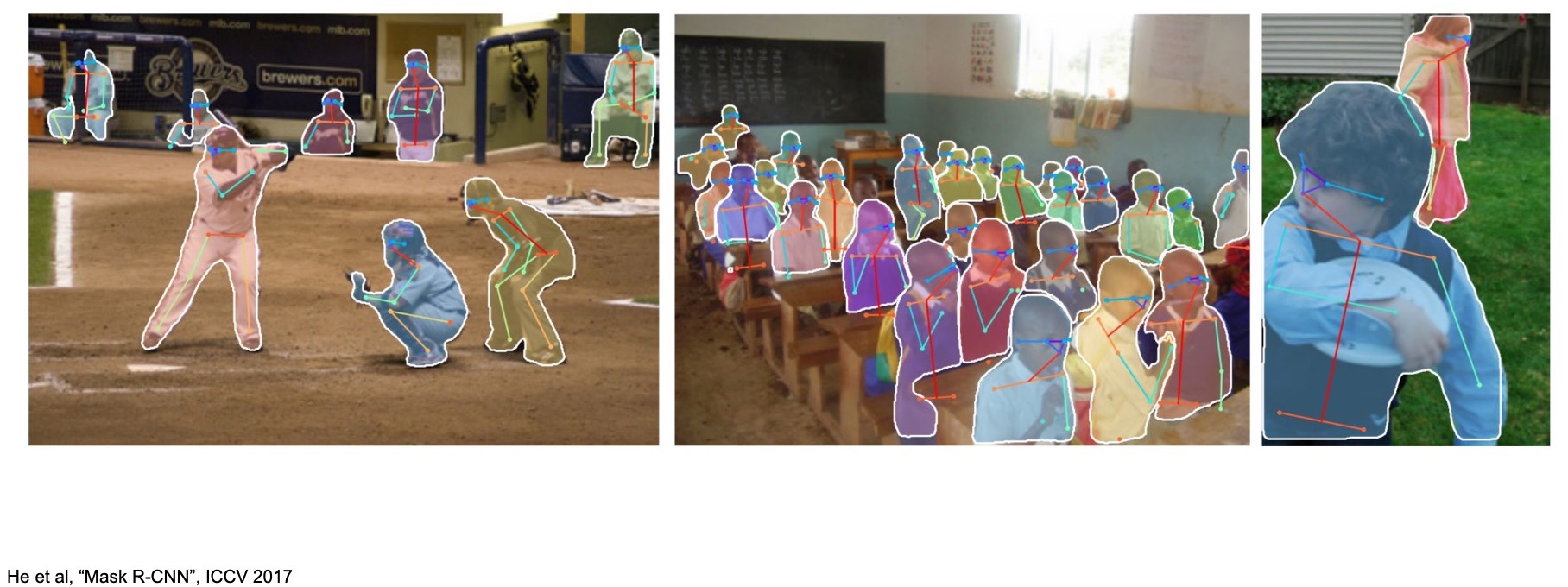
- You can also predict more fine-grained attributes such as human poses so this can be easily done by adding another output branch from the RoI Align layer and regress the key-pose location. Effectively, we’re doing as many regression objectives as the number of dots in each region proposal. This is thus, another auxiliary output from Mask R-CNN.
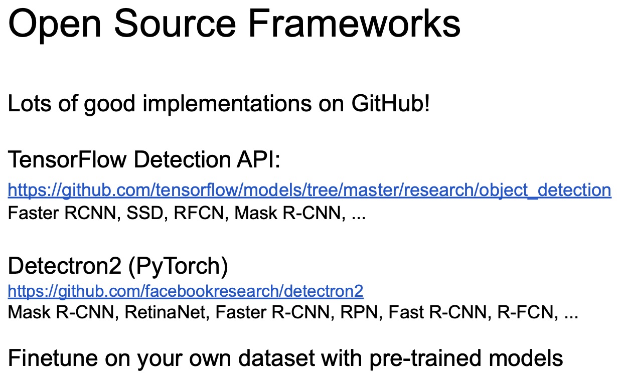
Open Source Frameworks
- There are a lot of open-source object detection and instance segmentation models. For e.g., the TensorFlow detection API includes a lot of the popular models which we discussed such as Faster R-CNN, SSD, RFCN, Mask R-CNN etc. For PyTorch, you have Detectron2 from Facebook AI Research (FAIR).
- Pretrained models on datasets such as COCO. Grab a model and fine-tune on your own dataset to train faster!
Beyond 2D Object Detection
Dense Image Captioning
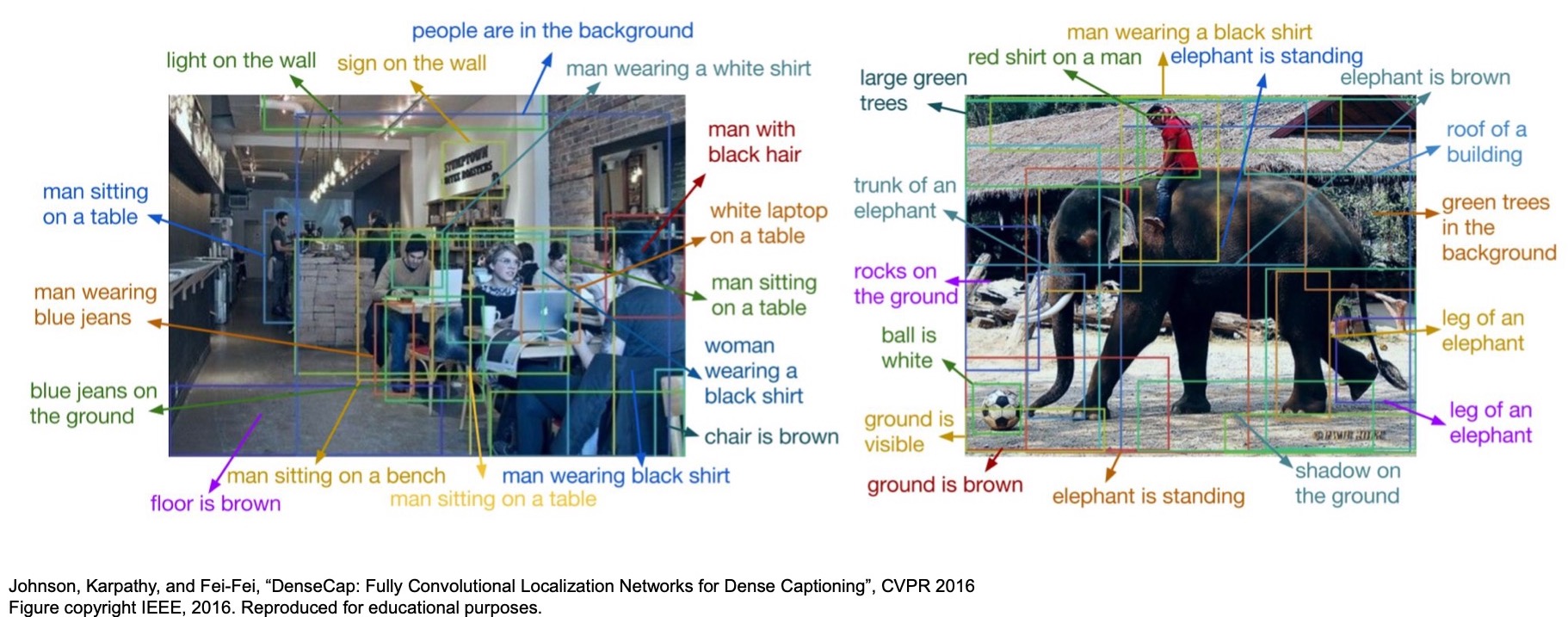
- Dense Captioning is an interesting problem that was introduced in “DenseCap: Fully Convolutional Localization Networks for Dense Captioning” (2015) by Johnson et al.
- Based on the ideas that we talked about for 2D object detection, we can do a lot more than just detect regions. Dense captioning is basically “Object Detection + Captioning”. For e.g., we can connect an RNN on top of the RPN from Faster R-CNN and generate natural language descriptions of the regions in an image, a task called Dense Image Captioning.
Dense Video Captioning
- “Dense-Captioning Events in Videos” (2017) by Krishna et al. applied the idea of dense captioning to videos by replacing the input branch with a 3D-convolutions-processed video source.
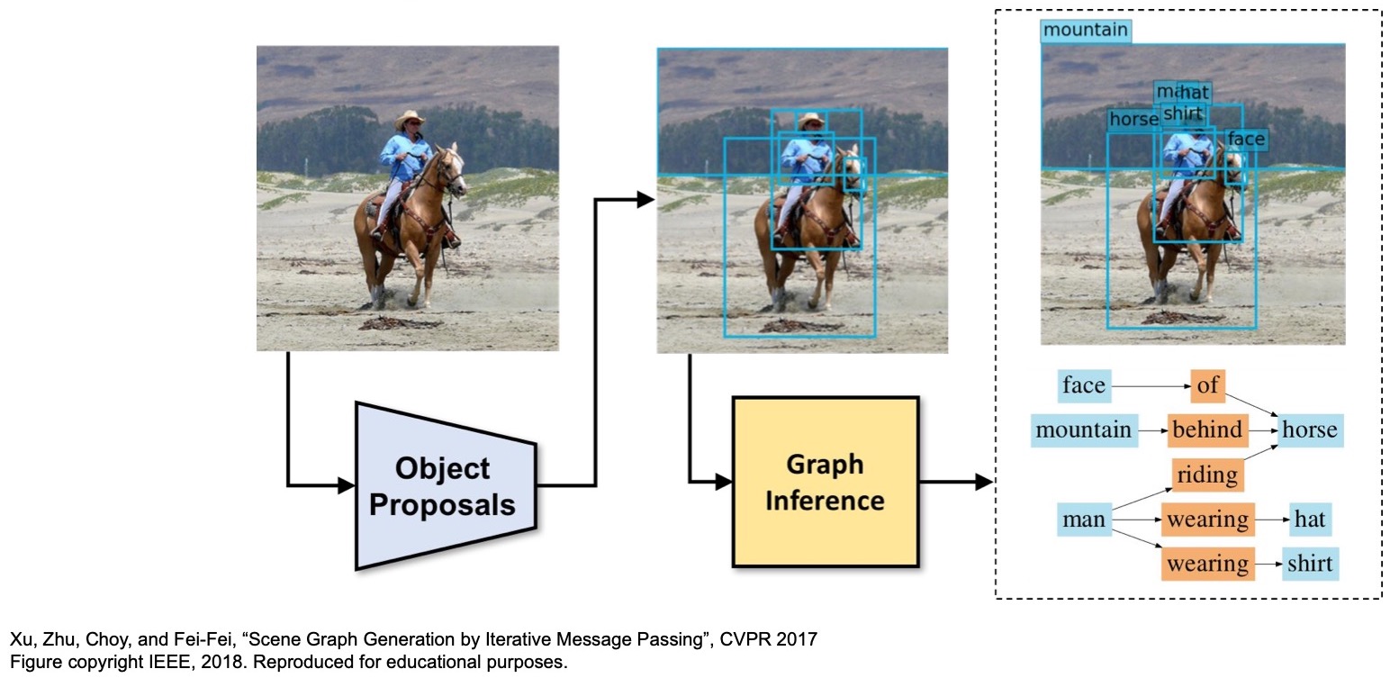
Scene Graphs
Objects + Relationships = Scene Graphs.
- The Visual Genome project essentially has a huge dataset offering a richer description of natural scenes such as relationships, region descriptions, attributes, etc.
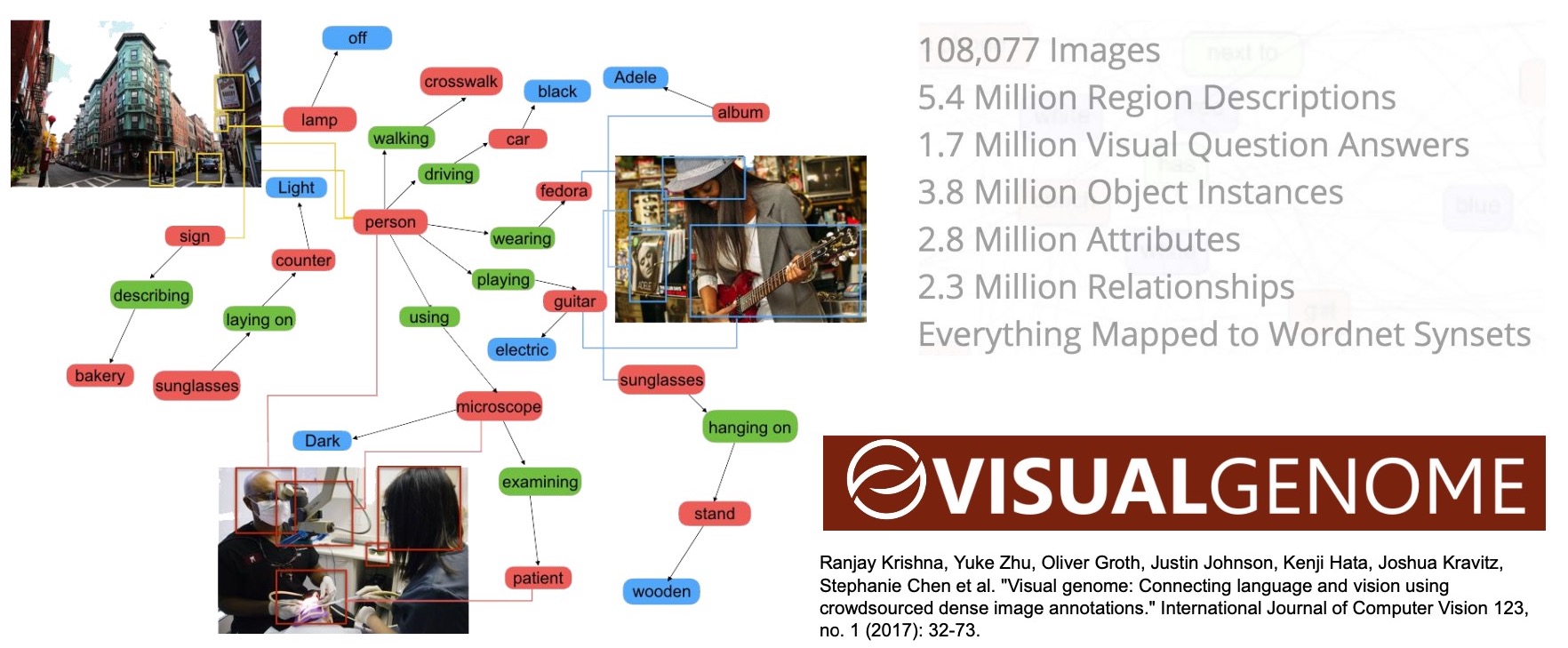
- By training a model on this dataset we can not only detect an object, but also understand their relationships among the objects.
- “Scene Graph Prediction” (2018) by Xu et al. builds a graph inference algorithm on top of the Faster R-CNN architecture and tries to predict both the object class and their semantic relationships.
3D Object Detection
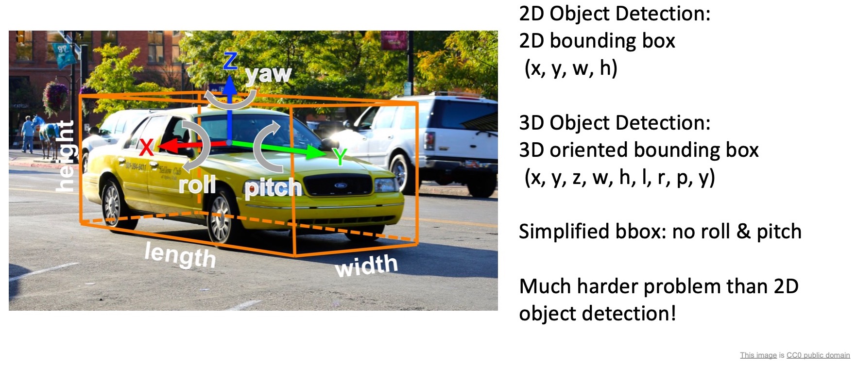
- The infrastructure that we developed for 2D object detection can be extended to 3D object detection. We can predict 3D bounding boxes in images to do 3D object detection. However, the problem here is a lot harder because 3D bounding boxes have a lot more parameters (shown below) and these numbers are no longer in pixel space. They are in the real-world space with a pre-determined co-ordinate system where these \((x,\,y,\,z)\)’s are actually meters on the \(roll\), \(pitch\) and \(yaw\) axes. So you have to parameterize the 3D bounding box with 9 numbers, namely \((x,\,y,\,z,\,w,\,h,\,l,\,r,\,p,\,y)\).
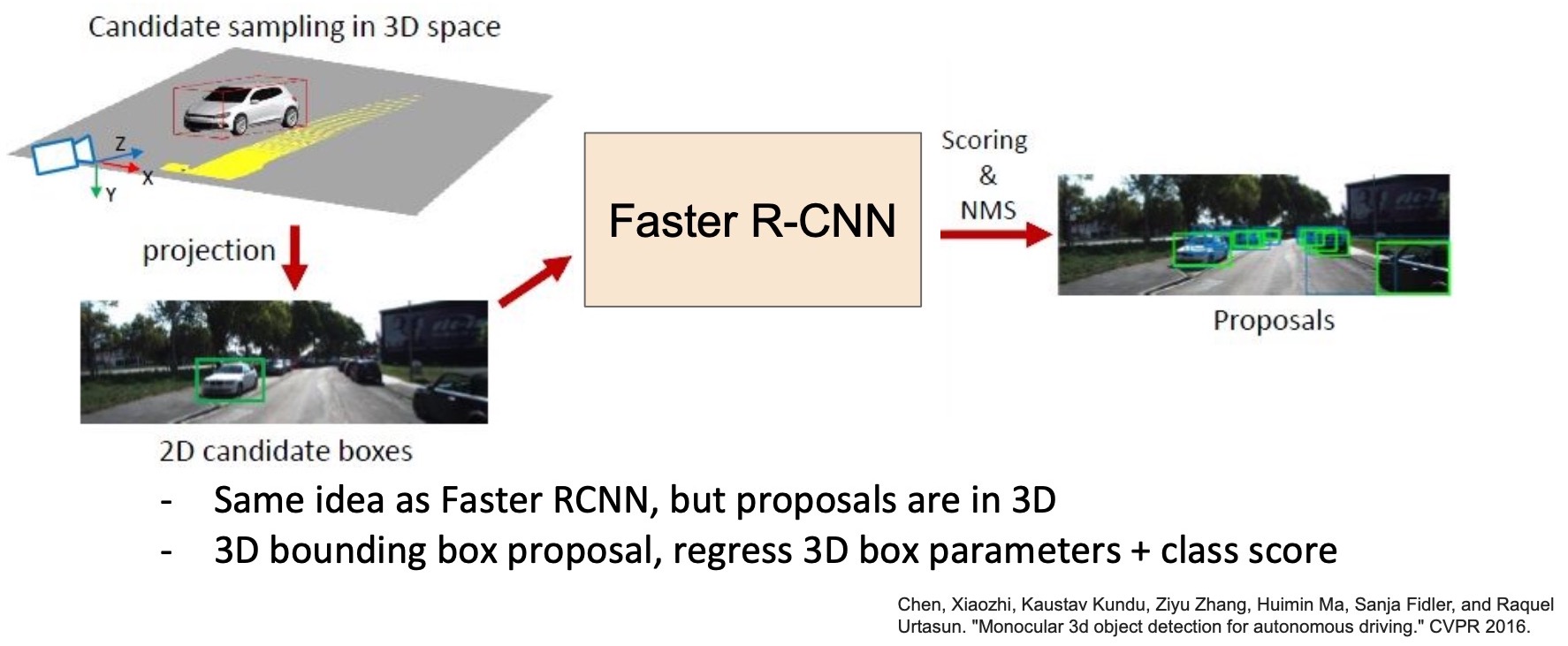
- The overall pipeline involves Faster R-CNN \(\rightarrow\) region proposals \(\rightarrow\) classification and regression of 9 numbers corresponding to the 3D bounding box. Of course, this approach is less performant compared to 2D object detection because the problem is inherently a lot more complex. However, recently, there has been a lot of work in the domain of 3D object detection, including leveraging sensor inputs such as LiDAR or depth cameras to improve accuracy.
3D Shape Prediction
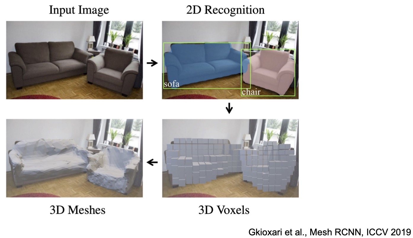
- Based on 3D object detection, Gkioxari et al. proposed “Mesh R-CNN” (2019) which predicts a mesh model for objects in the scene.
- Similar idea as earlier – uses region proposals for classification but you have another output for 3D voxels and meshes.
Key Takeaways
- In summary, we talked about:
- 3 of the biggest computer vision problems beyond classification, namely, object classification, semantic segmentation and instance segmentation.
- Semantic segmentation: where we want to label each pixel in an image with some category. We discussed a few ideas to achieve this goal and finally converged on the downsampling + upsampling architecture.
- Object detection: where we want to put bounding boxes around each object in the scene and this requires the model to make variable number of predictions for each image.
- Two-stage objection detectors: R-CNN -> Fast R-CNN -> Faster R-CNN -> Mask R-CNN.
- Single-stage object detectors: YOLO, SSD etc.
- Instance segmentation: achieved by building on top of detection algorithms to do semantic segmentation for each localized region.
- Lastly, we also talked about some research work that builds on the ideas of object detection such as dense captioning, scene graph generation, 3D object detection and shape prediction.
Citation
If you found our work useful, please cite it as:
@article{Chadha2020DistilledDetectionSegmentation,
  title   = {Detection and Segmentation},
  author  = {Chadha, Aman},
  journal = {Distilled Notes for Stanford CS231n: Convolutional Neural Networks for Visual Recognition},
  year    = {2020},
  note    = {\url{https://aman.ai}}
}