CS231n • Generative Models
- Overview
- Generative Models vs. Discriminative Models
- PixelRNN and PixelCNN
- Variational Autoencoders (VAEs)
- Generative Adversarial Networks (GANs)
- Transformer Decoder
- Diffusion Models
- Citation
Overview
Background
-
Generative models are a central topic in modern machine learning and artificial intelligence. Unlike models that only make predictions or classifications, generative models attempt to capture the underlying probability distribution of data. The idea is that if we can learn how the data is generated, we can then simulate or produce new examples that resemble the training data.
-
At a high level, a generative model learns the joint probability distribution:
\[p(x, y)\]-
where:
- \(x\) represents the input (such as an image, text, or audio),
- \(y\) may represent a label (in supervised contexts).
-
-
Once learned, such a model allows us to sample new data points \(x'\) that look like they come from the true data distribution.
Key Idea
- Generative models try to answer the question: “How is this data generated?”
-
They capture both the features and the relationships between them. For example:
- In image generation, a model should learn how pixels co-occur to form realistic images.
- In text generation, a model should capture grammar, semantics, and long-range dependencies.
- This contrasts with discriminative models (discussed in the next section), which instead focus on decision boundaries rather than modeling the data distribution itself.
Applications
-
Generative models have seen explosive growth in recent years, with applications in:
- Image synthesis (e.g., StyleGAN)
- Text generation (e.g., GPT models)
- Audio generation (e.g., WaveNet, Jukebox)
- Data augmentation for training
- Drug discovery and molecular design
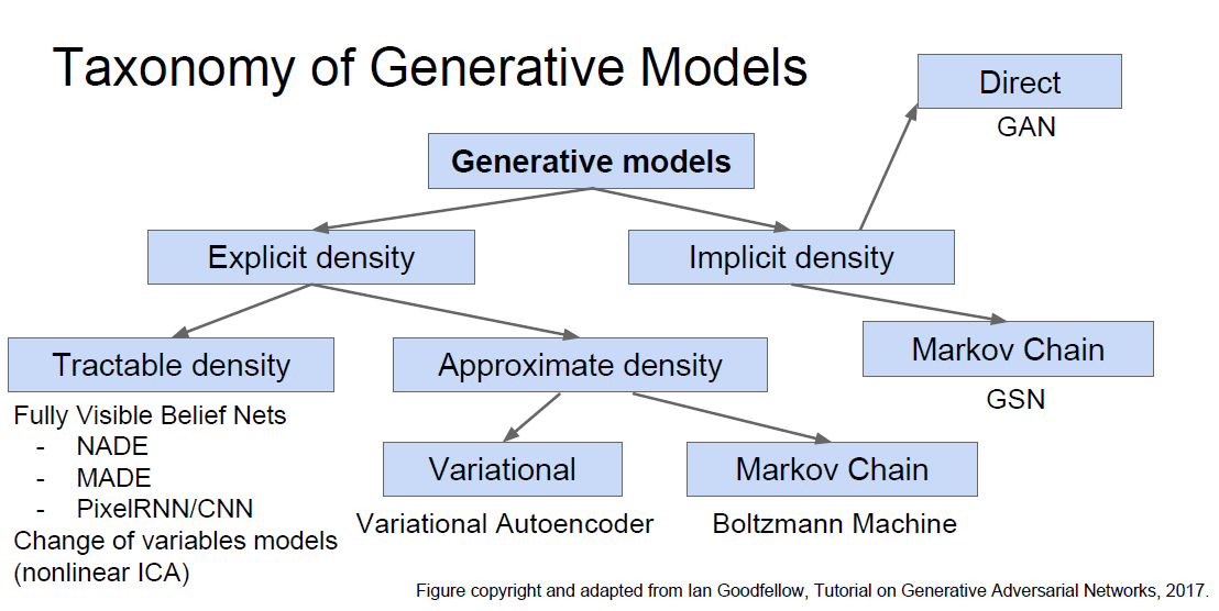
Taxonomy of Generative Models
- The following figure shows an overview of the taxonomy of generative models discussed in this chapter. The methods differ by whether they provide explicit likelihood estimation, implicit modeling, or rely on latent-variable inference.
Generative Models vs. Discriminative Models
Background
In machine le* arning, it is important to distinguish between generative and discriminative approaches. Both are powerful paradigms but serve different purposes. Understanding their differences provides context for why generative models are harder to train but offer broader applicability.
- Discriminative models: Learn the conditional probability distribution \(p(y \| x)\). They focus on decision boundaries and are used for tasks like classification.
- Generative models: Learn the joint distribution \(p(x, y)\) or directly model the data distribution \(p(x)\). They can generate new data points similar to the training data.
Formal Definitions
- Discriminative model:
- Learns how to map inputs to outputs by estimating
- Example: Logistic regression, Support Vector Machines (SVMs), or deep classifiers like ResNets.
- Generative model:
- Learns how the data is distributed, often modeling:
- Or, in unsupervised contexts, simply:
- Example: Variational Autoencoders (VAEs), Generative Adversarial Networks (GANs), and Diffusion Models.
Advantages and Limitations
-
Discriminative models
- Pros: Often achieve higher accuracy on supervised tasks, require fewer assumptions, and are easier to train.
- Cons: Cannot generate data, less flexible when data distribution shifts.
-
Generative models
- Pros: Can synthesize new data, useful for unsupervised or semi-supervised learning, can provide richer understanding of the data.
- Cons: Computationally more expensive, training is more complex (e.g., GAN instability, VAE approximations).
Intuition
- A discriminative model is like a judge who only cares about separating cats from dogs.
- A generative model is like an artist who tries to learn what cats and dogs look like, and can then draw new ones.
PixelRNN and PixelCNN
Background
-
One of the earliest families of deep generative models for images are autoregressive models, which generate pixels one at a time in a sequential manner. These models rely on the chain rule of probability, which allows the joint distribution over all pixels to be decomposed into a product of conditional probabilities.
-
For an image \(x\) with pixels \(x_1, x_2, \dots, x_n\), the distribution is modeled as:
- This framework ensures tractable likelihood estimation because each conditional distribution can be explicitly computed.
PixelRNN
-
Introduced in van den Oord et al., 2016, PixelRNN uses recurrent neural networks (RNNs) to model pixel dependencies.
- Idea: Scan through the image pixel-by-pixel (usually in a raster-scan order, left-to-right, top-to-bottom).
- Architecture: Uses LSTM-like units (Row LSTM, Diagonal BiLSTM) to capture long-range dependencies between pixels.
- Strengths: Captures complex dependencies, especially in structured regions of an image.
- Weaknesses: Sequential nature makes training and sampling slow.
PixelCNN
-
To address the inefficiency of PixelRNN, the same authors proposed PixelCNN in the same paper.
- Idea: Replace recurrent dependencies with masked convolutions.
- Masked convolution ensures that when predicting a pixel, the model only has access to already-generated pixels (causal structure).
- Strengths: Much faster to train and parallelize compared to PixelRNN.
- Weaknesses: While better at efficiency, it may capture dependencies less effectively compared to RNN-based models.
Key Equation
-
For PixelCNN, each conditional probability is parameterized by a CNN:
\[p(x_i | x_1, \dots, x_{i-1}) = \text{Softmax}(f_\theta(x_1, \dots, x_{i-1}))\]- where \(f_\theta\) is a masked convolutional neural network.
Extensions
- PixelCNN++ (Salimans et al., 2017): Improves PixelCNN by modeling pixel values with a mixture of logistics and using deeper architectures.
- Conditional PixelCNN: Allows conditioning on class labels or other side information, enabling class-conditional image generation.
Applications
- High-quality density estimation of natural images.
- Image completion (filling in missing pixels).
- Serving as likelihood benchmarks for evaluating generative models.
Variational Autoencoders (VAEs)
Background
-
Variational Autoencoders (VAEs), introduced by Kingma & Welling, 2013, are a class of generative models that combine probabilistic graphical models with deep learning. The key idea is to learn a low-dimensional latent representation of data while maintaining the ability to generate new samples.
-
VAEs are part of the latent variable models family. They assume that observed data \(x\) is generated from some latent variables \(z\) through a generative process:
\[p_\theta(x, z) = p_\theta(x|z)p(z)\]-
where:
- \(p(z)\) is typically a simple prior (e.g., standard Gaussian),
- \(p_\theta(x \| z)\) is a neural network that decodes latent variables into observed data.
-
The Challenge
-
The main difficulty is computing the marginal likelihood:
\[p_\theta(x) = \int p_\theta(x|z) p(z) \, dz\]- which is intractable for high-dimensional data.
Variational Inference
-
To address this, VAEs introduce an inference model \(q_\phi(z \| x)\) (the encoder), which approximates the true posterior \(p_\theta(z \| x)\).
-
Instead of maximizing \(\log p_\theta(x)\) directly, we optimize the Evidence Lower Bound (ELBO):
- The first term encourages accurate reconstruction of data.
- The KL divergence regularizes the approximate posterior to stay close to the prior.
Reparameterization Trick
- To backpropagate through stochastic sampling of \(z\), VAEs use the reparameterization trick:
- This allows gradients to flow through \(\mu_\phi(x)\) and \(\sigma_\phi(x)\), making the model trainable with standard stochastic gradient descent.
Architecture
- Encoder (Inference Network): Maps input \(x\) to parameters of \(q_\phi(z \| x)\).
- Latent Space: A compressed representation sampled from \(q_\phi(z \| x)\).
- Decoder (Generative Network): Maps latent variables \(z\) to reconstructed data.
Strengths and Weaknesses
- Pros: Provides a principled probabilistic framework, tractable training via ELBO, smooth latent space useful for interpolation.
- Cons: Generated samples often appear blurry due to Gaussian likelihood assumption; weaker sample quality compared to GANs.
Applications
- Image generation and interpolation.
- Semi-supervised learning.
- Representation learning in continuous latent spaces.
- Anomaly detection (using reconstruction error).
Generative Adversarial Networks (GANs)
Background
-
Generative Adversarial Networks (GANs), introduced by Goodfellow et al., 2014, are one of the most influential developments in generative modeling. GANs achieve remarkable success in synthesizing realistic images, videos, and even audio, often producing samples sharper than those generated by VAEs.
-
The key idea is to train two networks in a minimax game:
- A generator \(G(z; \theta_g)\) maps random noise \(z \sim p(z)\) (e.g., Gaussian) to synthetic data.
- A discriminator \(D(x; \theta_d)\) distinguishes between real data (from the training set) and fake data (from the generator).
Objective
- The GAN objective is formulated as:
- The discriminator tries to maximize the probability of correctly classifying real vs. fake data.
- The generator tries to minimize this objective, effectively “fooling” the discriminator.
Training Dynamics
- GAN training is notoriously unstable because the two networks are competing against each other.
- If \(D\) becomes too strong, \(G\) fails to learn. Conversely, if \(G\) dominates, \(D\) cannot improve.
- Variants such as Wasserstein GAN (WGAN) and Least Squares GAN (LSGAN) improve stability and sample quality.
Strengths and Weaknesses
- Pros: Capable of producing high-fidelity, sharp, and realistic samples. Widely successful in image generation and manipulation.
- Cons: Training instability, mode collapse (generator produces limited diversity), lack of an explicit likelihood estimate.
Extensions and Variants
-
GAN research has exploded into numerous variants, addressing stability, scalability, and conditioning:
- Conditional GANs (cGANs): Generate data conditioned on labels or attributes.
- DCGAN: Deep convolutional GAN, one of the earliest stable architectures.
- CycleGAN: Enables unpaired image-to-image translation (e.g., horses ↔ zebras).
- StyleGAN: Known for high-quality face generation and controllable style transfer.
-
For a detailed collection, see the GAN Zoo.
Practical Tips
- Training GANs is difficult, but practitioners have compiled best practices such as architectural choices, optimizer settings, and regularization tricks. See GAN hacks for a curated set of guidelines.
Learning Resources
- The NIPS 2016 GAN Tutorial by Ian Goodfellow remains one of the most accessible introductions to GANs.
Applications
- Image synthesis (faces, artwork, super-resolution).
- Data augmentation in medical imaging.
- Text-to-image generation (e.g., DALL·E-style systems).
- Video generation and frame prediction.
- Style transfer and domain adaptation.
Transformer Decoder
Background
- Transformers, introduced in Vaswani et al., 2017, revolutionized sequence modeling by replacing recurrence with self-attention mechanisms. This architecture has since become the foundation for large-scale language models (e.g., GPT, BERT, T5) and generative systems across text, vision, and multimodal domains.
- The Transformer consists of an encoder-decoder structure. In the context of generative modeling, the decoder is of particular importance, as it is responsible for autoregressively generating sequences.
- For a detailed discourse on the Transformer architecture, please refer to our Transformer primer and LLM primer.
Self-Attention Mechanism
- At the heart of the Transformer is scaled dot-product attention. Given queries \(Q\), keys \(K\), and values \(V\):
- This allows each position in the sequence to attend to all previous positions, enabling long-range dependencies without recurrence.
Decoder Architecture
-
The Transformer decoder is composed of stacked layers, each containing:
-
Masked Multi-Head Self-Attention
- Ensures autoregressive property by masking future tokens.
- Each token can only attend to tokens before it.
-
Cross-Attention (to Encoder Outputs, in seq-to-seq tasks)
- Not present in pure autoregressive models like GPT.
- Enables conditioning on input sequences (e.g., for translation).
-
Feed-Forward Neural Network (FFN)
- Position-wise fully connected layers applied after attention.
-
-
Each sub-layer is wrapped with residual connections and layer normalization.
Positional Encoding
- Since self-attention is permutation-invariant, Transformers add positional encodings to input embeddings to inject sequence order:
- This allows the model to capture relative and absolute positions of tokens.
Why the Decoder Matters for Generation
-
In language modeling, the decoder predicts the next token given all previous tokens:
\[p(x) = \prod_{t=1}^T p(x_t | x_{<t})\] -
The autoregressive nature makes it ideal for text generation, but the same principle extends to audio, video, and multimodal synthesis.
Strengths and Weaknesses
- Pros: Parallelizable training, strong long-range dependency modeling, scalability to billions of parameters.
- Cons: High computational cost (quadratic in sequence length due to attention), challenges in efficiency for very long contexts.
Applications
- Language models (GPT-family, PaLM, LLaMA).
- Text-to-image (paired with diffusion or GAN components).
- Speech and music generation.
- Multimodal generative systems (e.g., CLIP + Transformer decoders).
Diffusion Models
Background
- Diffusion models are a class of generative models that have recently achieved state-of-the-art results in image, audio, and video synthesis. Popularized by works such as DDPM: Ho et al., 2020 and subsequent improvements (e.g., DDIM, Latent Diffusion Models), these models generate data by gradually denoising a random noise vector into a coherent sample.
- The underlying inspiration comes from non-equilibrium thermodynamics: data is progressively diffused into noise through a forward process, and the generative model learns to reverse this process. For a detailed discourse on Diffusion Models, please refer to our Diffusion Models primer.
Forward Diffusion Process
-
In the forward process, data is corrupted step-by-step with Gaussian noise:
\[q(x_t | x_{t-1}) = \mathcal{N}(x_t; \sqrt{1-\beta_t}x_{t-1}, \beta_t I)\]-
where:
- \(x_0\) is the original data,
- \(\beta_t\) is a small noise variance schedule.
-
-
After many steps, \(x_T\) becomes nearly pure Gaussian noise.
Reverse Denoising Process
-
The generative model learns the reverse distribution:
\[p_\theta(x_{t-1} | x_t) = \mathcal{N}(x_{t-1}; \mu_\theta(x_t, t), \Sigma_\theta(x_t, t))\]- where a neural network parameterized by \(\theta\) predicts the noise added at each step.
-
Training objective often reduces to predicting the noise \(\epsilon\) added during the forward process, leading to a simplified loss:
Sampling
- Start from pure noise \(x_T \sim \mathcal{N}(0, I)\).
- Iteratively denoise using the learned reverse process until reaching \(x_0\).
- Results in high-fidelity samples with controllable generation.
Extensions
- DDIM (Denoising Diffusion Implicit Models): Speeds up sampling with fewer steps.
- Latent Diffusion Models (LDMs): Apply diffusion in a compressed latent space (e.g., Stable Diffusion) for efficiency.
- Guided Diffusion: Conditioning mechanisms (e.g., classifier guidance, text conditioning with CLIP).
Strengths and Weaknesses
- Pros: Exceptional sample quality, strong mode coverage, stable training compared to GANs.
- Cons: Slow sampling due to many denoising steps (though recent research improves efficiency).
Applications
- Image generation (Stable Diffusion, DALL·E 2, Imagen).
- Text-to-image and image-to-image tasks.
- Audio generation (speech synthesis, music).
- Video generation.
Citation
If you found our work useful, please cite it as:
@article{Chadha2020GenerativeModels,
  title   = {Generative Models},
  author  = {Chadha, Aman},
  journal = {Distilled Notes for Stanford CS231n: Convolutional Neural Networks for Visual Recognition},
  year    = {2020},
  note    = {\url{https://aman.ai}}
}