CS229 • Locally Weighted Linear Regression
- Fitting your data
- Feature selection algorithms
- Locally weighted linear regression
- Parametric vs. non-parametric learning
- References
- Citation
Fitting your data
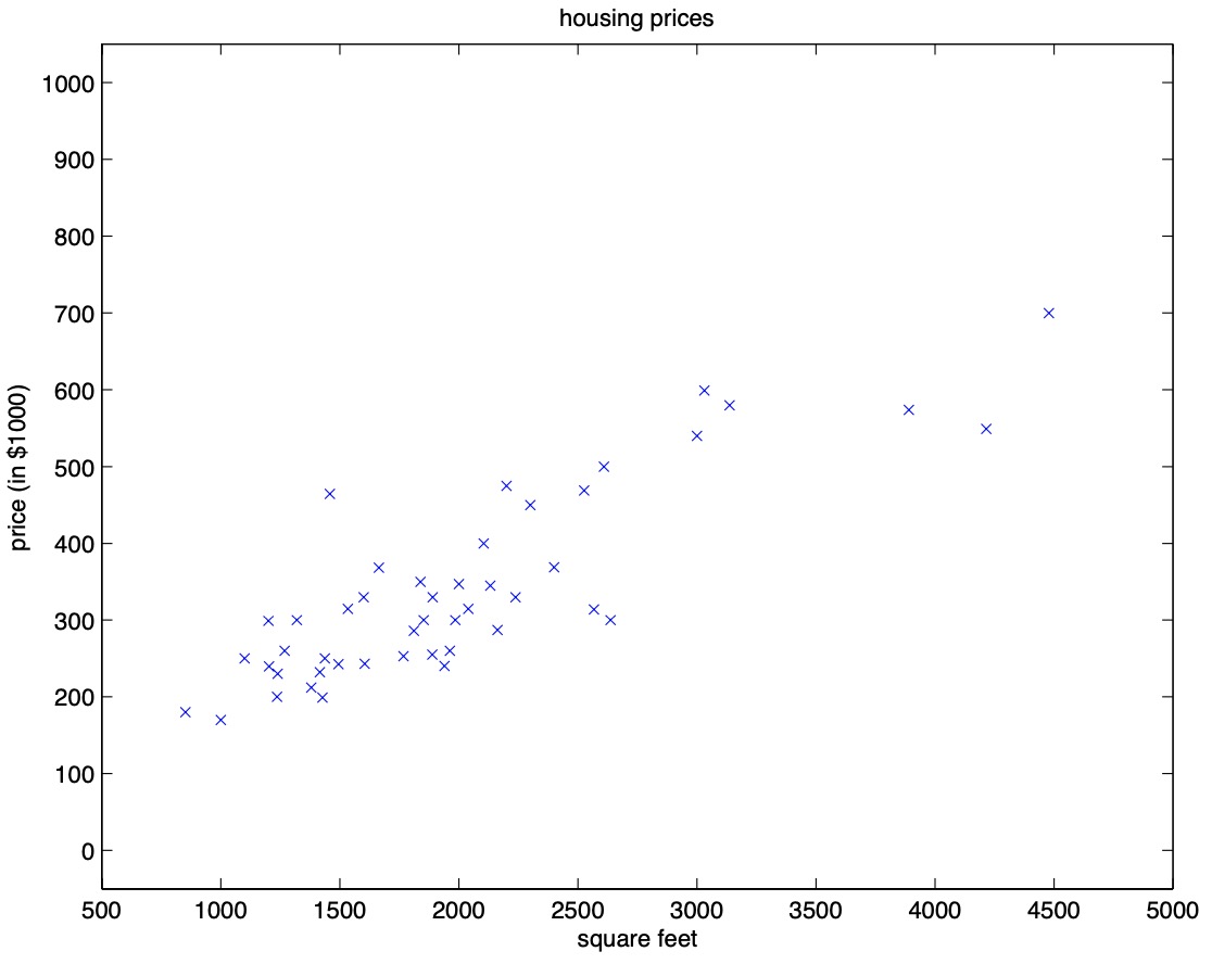
- Consider the supervised learning problem of predicting house prices that we reviewed in the topic of linear regression. Assume you’re given the housing prices dataset that we looked at earlier, that shows how the price of a house varies with its size:
- A question that you have to address when trying to fitting models to data is: what are the features that you want?
- We can either fit…
- A straight line fit of the form \(\theta_0 + \theta_{1}{x_1}\).
- A quadratic fit of the form \(\theta_0 + \theta_{1}{x_1} + \theta_{2}{x_2}^2\).
- Or maybe you would like a custom fit such as \(\theta_0 + \theta_{1}{x} + \theta_{2} \sqrt{x} + \theta_{3} \log{x}\).
- To implement this, you would define the first feature \(x_1 = x\), second feature \(x_2 = \sqrt{x}\) and third feature \(x_3 = \log{x}\).
- By defining these new features \(x_1\), \(x_2\) and \(x_3\), the machinery of linear regression lends itself naturally to fit these functions of input features in your dataset.
Feature selection algorithms
- Feature selection algorithms are algorithms for automatically deciding the best set of features for fitting your data.
- In other words, feature selection algorithms help answer the question: What combination of functions of your input features would yield the best performance?
- In other words, which functions of \(x\), say \(x^2\), \(\sqrt{x}\), \(\log{x}\), \(x^3\), \(\sqrt[^3]{x}\) or \(x^{\frac{2}{3}}\), are appropriate features to use? If so, what combination do we string them together with?
- To fit a dataset that is inherently non-linear, a straight line wouldn’t be the best choice and we’d have to explore polynomials.
- To tackle the problem of fitting data that is non-linear and figuring out the best combination of the functions of your features to use, locally weighted regression comes in play.
Locally weighted linear regression
- In this section, we shall discuss locally weighted regression, an algorithm that modifies linear regression to make it fit non-linear functions.
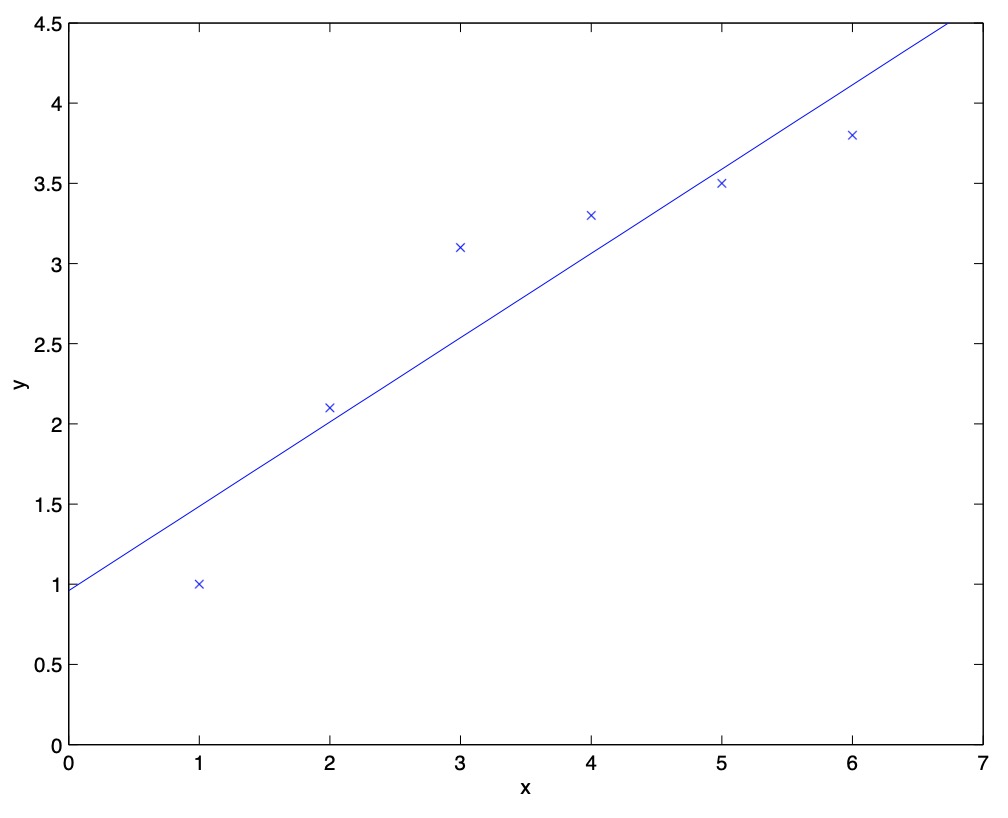
- Consider the problem of predicting \(y\) from \(x \in \mathbb{R}\), as shown in the figure below. The leftmost figure below shows the result of fitting a \(y = \theta_0 + \theta_1 x\) to a dataset. We see that the data doesn’t really lie on straight line, and so the fit is not very good.
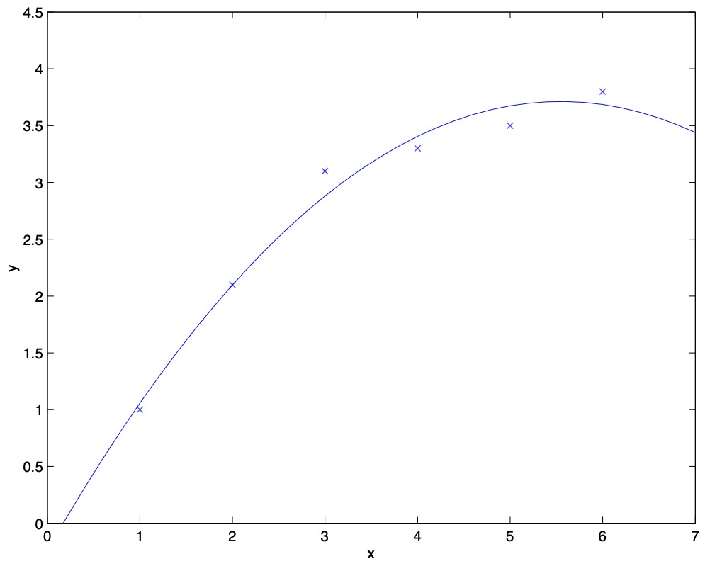
- Instead, if we had added an extra feature \(x^2\), and fit \(y = \theta_0 + \theta_1 x + \theta_2 x^2\), then we obtain a slightly better fit to the data (cf. figure below).
- Naively, it might seem that the more features we add, the better. However, there is also a danger in adding too many features. The figure below is the result of fitting a \(5^{th}\) order polynomial \(y = \sum_{j = 0}^5 \theta_j x^j\). We see that even though the fitted curve passes through the data perfectly, we would not expect this to be a very good predictor of, say, housing prices \(y\) for different living areas \(x\).
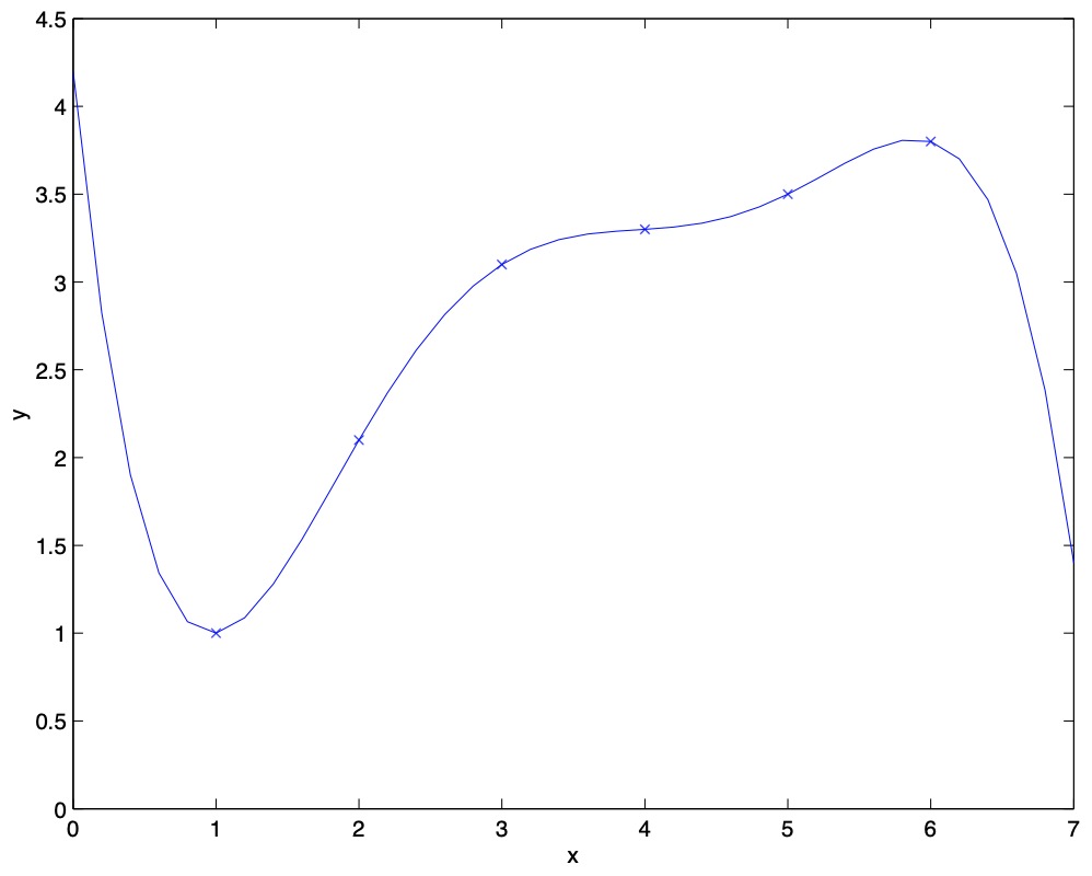
- Without formally defining what these terms mean, we’ll say the figure on the left shows an instance of underfitting – in which the data clearly shows structure not captured by the model – and the figure on the right is an example of overfitting.
- As shown in the diagram above, the choice of features is important to ensuring good performance of a learning algorithm. Let’s delve into the locally weighted linear regression (LWR) algorithm which, assuming there is sufficient training data, makes the choice of features less critical.
- In the original linear regression algorithm, you train your model by fitting \(\theta\) to minimize your cost function \(J(\theta) = \frac{1}{2} \sum_i (y^{(i)} - \theta^T x^{(i)})^2\). To make a prediction, i.e., to evaluate your hypothesis \(h_{\theta}(x)\) at a certain input \(x\), simply return \(\theta^T x\).
- In contrast, to make a prediction at an input \(x\) using locally weighted linear regression:
- Look into the local neighborhood (similar input values) of the training examples close to \(x\). Focus mainly on these examples, and fit a straight line through them.
- Fit a line passing through the outputs \(y\) in that neighborhood, and make a prediction at \(x\).
- Note that by focusing on the local neighborhood of input points, we attribute these points to influence the output prediction the most, but the other points can also be weighted lesser and utilized for our prediction.
-
To formalize this, locally weighted regression fits \(\theta\) to minimize a modified cost function \(J(\theta)\):
\[J(\theta) = \sum_i^m w^{(i)}(y^{(i)} - \theta^T x^{(i)})^2\]- where \(w^{(i)}\) is a “weighting” function which yields a value \(\in [0, 1]\) that tells you how much should you pay attention to, i.e., weigh, the values of \((x^{(i)}, y^{(i)})\) when fitting a line through the neighborhood of \(x\).
-
A common choice for \(w^{(i)}\) is:
\[w^{(i)} = exp \left(-\frac{(x^{(i)} - x)^2}{2\tau^2}\right)\]- where,
- \(x\) is the input for which you want to make a prediction.
- \(x^{(i)}\) is the \(i^{th}\) training example.
- where,
- Note that the formula for \(w^{(i)}\) has a defining property:
- If \(|x^{(i)} - x|\) is small, i.e., \(x^{(i)}\) represents a training example that is close to \(x\), then the weight for that sample \(w^{(i)} \approx e^0 = 1\). Thus, when then picking \(\theta\), we’ll try hard to make \((y^{(i)} − \theta^T x^{(i)})^2\) small.
- Conversely, if \(|x^{(i)} - x|\) is large, i.e., \(x^{(i)}\) represents a training example that is far away from \(x\), then the weight for that sample \(w^{(i)} = e^{\text{large negative number}} \approx 0\). This implies that the error term \((y^{(i)} − \theta^T x^{(i)})^2\) would be pretty much ignored in the fit.
- Also, note that while the formula for the weights \(w^{(i)}\) takes a form that is cosmetically similar to the density of a Gaussian distribution (i.e., has the shape of a Gaussian bell curve), the \(w^{(i)}\)’s do not directly have anything to do with Gaussians, and in particular the \(w^{(i)}\) are not random variables, normally distributed or otherwise. So, \(w^{(i)}\) is just a function that is shaped a lot like a Gaussian, but Gaussian probability density functions integrate to 1 and this does not.
- Geometrically interpreting the \(w^{(i)}\) curve, the weight of the individual samples in the neighborhood of \(x\) are essentially represented by the height of the \(w^{(i)}\) curve at that point. Since the curve is centered at \(x\), the samples closest to \(x\) are weighted the most, while the samples far away from \(x\) are attributed the least weights.
Bandwidth parameter
- The bandwidth parameter \(\tau\) decides the width of the neighborhood you should look into to fit the local straight line.
- In other words, \(\tau\) controls how quickly the weight of a training example \(x^{(i)}\) falls off with distance from the query point \(x\). Depending on the choice of \(\tau\), you choose a fatter or thinner bell-shaped curve, which causes you to look in a bigger or narrower window respectively, which in turn decides the number of nearby examples to use in order to fit the straight line.
- \(\tau\) has an effect on overfitting and underfitting:
- If \(\tau\) is too broad, you end up over-smoothing the data leading to underfitting.
- If \(\tau\) is too thin, you end up fitting a very jagged fit to the data leading to overfitting.
- \(\tau\) is a hyper-parameter of the locally weighted regression algorithm.
- There’s a huge literature on choosing \(\tau\). For example, instead of the bell-shaped curve, a triangle shaped function can be used so your weights actually go to zero outside some small range. So there are many versions of this algorithm.
Cost function intuition
- Looking at the cost function, the main modification to the cost function we’ve made is that we’ve added the weighting term \(w^{(i)}\).
- Thus, intuitively, what locally weighted regression is saying is that if an example \(x^{(i)}\) is far from where you want to make a prediction, multiply that error term by a constant \(\approx 0\), whereas if it’s close to where you want to make a prediction, multiply that error term by \(\approx 1\).
- Since the terms multiplied by 0 essentially disappear as far as the summation is concerned, the net effect of this is that the squared error summation happens only over the terms for the examples that are close to the value \(x\) where you want to make a prediction.
- Thus, when you fit \(\theta\) to minimize your modified cost function, you end up paying attention, i.e., attributing a much higher weight, to the errors on training examples close to your query point \(x\).
Applications
- The major benefit of locally weighted regression is that fitting a non-linear dataset doesn’t require fiddling manually with features.
- Locally weighted linear regression is useful when you have a relatively low dimensional dataset, i.e., when the number of features \(n\) isn’t too large, say 2 or 3.
- Note that there are also constraints on the amount of data that locally weighted linear regression can handle from a computational complexity perspective. The computation needed to fit the minimization is similar to the normal equations, and so it involves solving a linear system of equations of dimension equal to the number of training examples you have.
- If you have a few thousands of examples, the computation involved is usually tractable.
- If you have tens of millions of examples, then we have to resort to scaling algorithms like KD trees.
- However, as we will see from our discussion in the upcoming section on parametric vs. non-parametric learning, the space complexity involved with locally weighted linear regression scales linearly with the number of training examples.
Parametric vs. non-parametric learning
Linear regression
- With a parametric learning algorithm, you fit a fixed set of parameters \(\theta\) to your data.
- The (unweighted) linear regression is a parametric learning algorithm.
- No matter how big your training set is, once you train your model and fit the parameters, you could erase the entire training set from memory and make predictions just using the parameters \(\theta\). Your parameters thus represent a summary of your original dataset.
Locally weighted linear regression
- Locally weighted regression is a non-parametric learning algorithm. The amount of data you need to keep around to represent the hypothesis \(h(\cdot)\), grows with the size of the training set. In case of locally weighted regression, this growth rate is linear.
Non-parametric algorithms are not ideal if you have a massive dataset because you need to keep all of the data around in computer memory or on disk just to make predictions.
References
Citation
If you found our work useful, please cite it as:
@article{Chadha2020DistilledLocallyWeightedLinearRegression,
  title   = {Locally Weighted Linear Regression},
  author  = {Chadha, Aman},
  journal = {Distilled Notes for Stanford CS229: Machine Learning},
  year    = {2020},
  note    = {\url{https://aman.ai}}
}