CS229 • Linear Regression
- Overview
- Notation
- Supervised learning
- Linear regression
- The normal equations
- Probabilistic interpretation: why squared error?
- Likelihood vs. probability
- References
- Citation
Overview
- This section covers:
- Supervised learning using linear regression.
- Batch and stochastic gradient descent as algorithms for fitting linear regression models.
- Normal equation as an efficient way to fit linear models.
Notation
- \(x^{(i)}\) denotes the input variables or features, and \(y^{(i)}\) denotes the output or target variable that we’re trying to predict, where the superscript \(“(i)”\) denotes the \(i^{th}\) training sample.
- Note that the superscript \(“(i)”\) in the notation is simply an index into the training set, and has nothing to do with exponentiation.
- A pair \((x^{(i)}, y^{(i)})\) denotes a single training example.
- \(x^{(i)} \in \mathbb{R}^{n + 1}\), i.e., \(x^{(i)}\) is \(n + 1\) dimensional, while \(y^{(i)} \in \mathbb{R}\), i.e., \(y^{(i)}\) is a single real number.
- So if you have two features, say the size of the house and the number of bedrooms, then \(x^{(i)}\) would be 2 + 1 = 3-dimensional.
- The additional feature beyond the \(n\) input features is due to the fact that we introduced a “fake” feature \(x_0\) which was always set to the value of 1.
- \(y^{(i)}\) in the case of regression is always a real number.
- \(x_j^{(i)}\) represents the \(j^{th}\) feature of the \(i^{th}\) training sample.
- \(m\) denotes the number of training examples.
- \(n\) denotes the number of features.
- The dataset that we’ll be using to learn – a list of \(m\) training examples \({(x^{(i)}, y^{(i)}); i = 1, \ldots, m}\), is called a training set.
- \(h_{\theta}(x)\) denotes the hypothesis function, which is a linear function of the features \(x\) and \(x_0 = 1\).
- \(J_{\theta}\) denotes the cost function you’re looking to minimize, to find the optimal set of parameters \(\theta\) for your straight line fit to the data.
- \(\mathcal{X}\) denotes the space of input values, while \(\mathcal{Y}\) denotes the space of output values. For e.g., if both the input features and output are real numbers, then \(\mathcal{X}=\mathcal{Y}=\mathbb{R}\).
Supervised learning
- Let’s start by talking about a few examples of supervised learning problems. Suppose we have a dataset giving the living areas and prices of 47 houses from Portland, Oregon:
| \(\text{Living area }(feet^2)\) | \(\text{Price }(1000\$’s)\) |
|---|---|
| 2104 | 400 |
| 1600 | 330 |
| 2400 | 369 |
| 1416 | 232 |
| 3000 | 540 |
| \(\vdots\) | \(\vdots\) |
- Plotting this data yields:
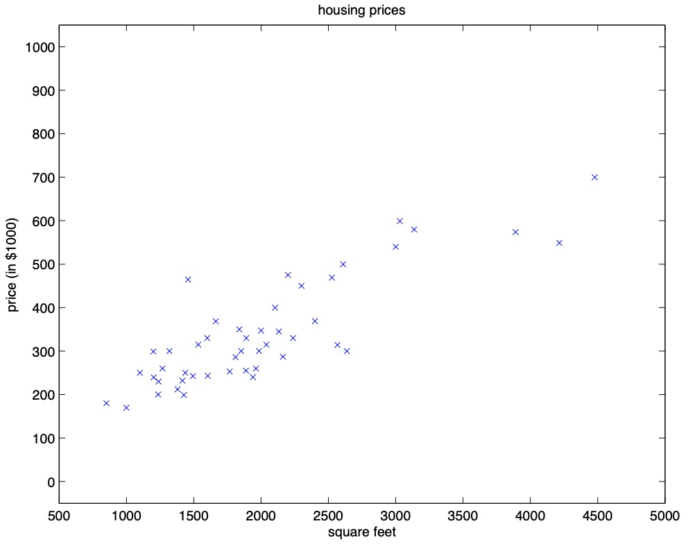
- Thus, the question arises: given the above dataset, how can we learn to predict the prices of other houses in Portland, as a function of the size of their living areas?
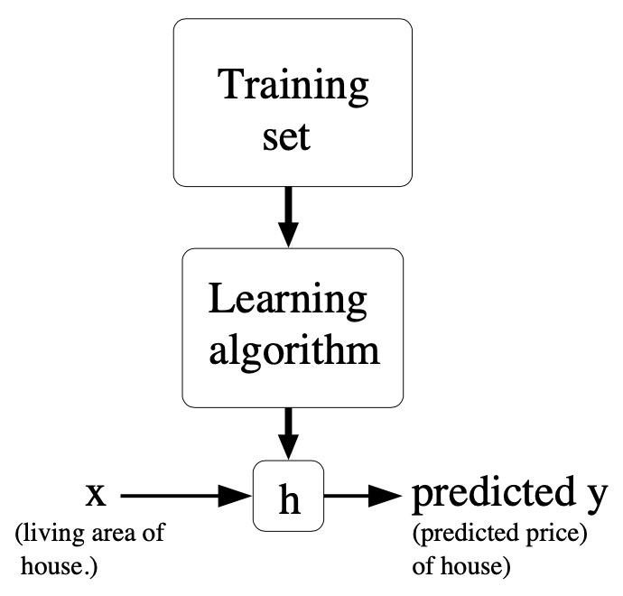
- A formal definition of the supervised learning problem is as follows. Given a training set our goal is to learn a function \(h: \mathcal{X} \mapsto \mathcal{Y}\) so that \(h(x)\) is a “good” predictor for the corresponding value of \(y\). For historical reasons, this function \(h(\cdot)\) is called a hypothesis. Seen pictorially, the process is therefore like this:
- When the target variable that we’re trying to predict is continuous, such as in our housing example, we call the learning problem a regression problem. When \(y\) can take on only a small number of discrete values (such as if, given the living area, we wanted to predict if a dwelling is a house or an apartment, say), we call it a classification problem.
Linear regression
- To make our housing example more interesting, let’s consider a slightly richer dataset in which we also know the number of bedrooms in each house:
| \(\text{Living area }(feet^2)\) | \(\text{Bedrooms }(\#)\) | \(\text{Price }(1000\$’s)\) |
|---|---|---|
| 2104 | 3 | 400 |
| 1600 | 3 | 330 |
| 2400 | 3 | 369 |
| 1416 | 2 | 232 |
| 3000 | 4 | 540 |
| \(\vdots\) | \(\vdots\) | \(\vdots\) |
- Here, the \(x\)’s are two-dimensional vectors in \(\mathbb{R}^{2}\). For instance, \(x_{1}^{(i)}\) is the living area of the \(i^{th}\) house in the training set, and \(x_{2}^{(i)}\) is its number of bedrooms.
- In general, when designing a learning problem, it will be up to you to decide what features to choose, so if you are out in Portland gathering housing data, you might also decide to include other features such as whether each house has a fireplace, the number of bathrooms, and so on. We’ll say more about feature selection later, but for now let’s take the features as given.
- To perform supervised learning, we must decide how we’re going to represent functions/hypotheses \(h\) in a computer. As an initial choice, let’s say we decide to approximate \(y\) as a linear function of \(x\):
-
Here, the \(\theta_{i}\)’s are the parameters (also called weights) parameterizing the space of linear functions mapping from \(\mathcal{X}\) to \(\mathcal{Y}\). When there is no risk of confusion, we will drop the \(\theta\) subscript in \(h_{\theta}(x)\), and write it more simply as \(h(x)\). To simplify our notation, we also introduce the convention of letting \(x_{0}=1\) (this is the intercept term) such that,
\[h(x)=\sum_{i=0}^{n} \theta_{i} x_{i}=\theta^{T} x\]- where,
- On the right-hand side above we are viewing \(\theta\) and \(x\) both as vectors.
- \(n\) is the number of input variables (not counting \(x_{0}\)).
- where,
-
Now, given a training set, how do we pick, or learn, the parameters \(\theta\)? One reasonable method seems to be to make \(h(x)\) close to \(y\), at least for the training examples we have. To formalize this, we will define a function that measures, for each value of the \(\theta\)’s, how close the \(h(x^{(i)})\)’s are to the corresponding \(y^{(i)}\)’s. We define the cost function:
- If you’ve seen linear regression before, you may recognize this as the familiar least-squares cost function that gives rise to the ordinary least squares regression model. Whether or not you have seen it previously, let’s keep going, and we’ll eventually show this to be a special case of a much broader family of algorithms.
LMS algorithm
- We want to choose \(\theta\) so as to minimize \(J(\theta)\). To do so, let’s use a search algorithm that starts with some “initial guess” for \(\theta\), and that repeatedly changes \(\theta\) to make \(J(\theta)\) smaller, until hopefully we converge to a value of \(\theta\) that minimizes \(J(\theta)\). Specifically, let’s consider the gradient descent algorithm, which starts with some initial \(\theta\), and repeatedly performs the update:
- This update is simultaneously performed for all values of \(j=0, \ldots, n\). Here, \(\alpha\) is called the learning rate. This is a very natural algorithm that repeatedly takes a step in the direction of steepest decrease of \(J(\theta)\).
- In order to implement this algorithm, we have to work out what is the partial derivative term on the right-hand side. Let’s first work it out for the case of if we have only one training example \((x, y)\), so that we can neglect the sum in the definition of \(J(\theta)\). We have:
- For a single training example, this gives the update rule:
- Note that we use the notation \(“a:=b”\) to denote an operation (in a computer program) in which we set the value of a variable \(a\) to be equal to the value of \(b\). In other words, this operation overwrites \(a\) with the value of \(b\). In contrast, we will write \(“a=b”\) when we are asserting a statement of fact, that the value of \(a\) is equal to the value of \(b\).
- The rule is called the LMS update rule (LMS stands for “least mean squares”), and is also known as the Widrow-Hoff learning rule. This rule has several properties that seem natural and intuitive. For instance, the magnitude of the update is proportional to the error term \(\left(y^{(i)}-h_{\theta}(x^{(i)})\right)\); thus, for instance, if we are encountering a training example on which our prediction nearly matches the actual value of \(y^{(i)}\), then we find that there is little need to change the parameters; in contrast, a larger change to the parameters will be made if our prediction \(h_{\theta}(x^{(i)})\) has a large error (i.e., if it is very far from \(y^{(i)}\)).
- We’d derived the LMS rule for when there was only a single training example. There are two ways to modify this method for a training set of more than one example. The first is replace it with the following algorithm:
-
Repeat until convergence, for every \(j\):
\[\theta_{j}:=\theta_{j}+\alpha \sum_{i=1}^{m}\left(y^{(i)}-h_{\theta}\left(x^{(i)}\right)\right) x_{j}^{(i)}\]
-
- The reader can easily verify that the quantity in the summation in the update rule above is just \(\frac{\partial J(\theta)}{\partial \theta_{j}}\) (for the original definition of \(J(\theta)\)). So, this is simply gradient descent on the original cost function \(J(\theta)\). This method looks at every example in the entire training set on every step, and is called batch gradient descent. Note that, while gradient descent can be susceptible to local minima in general, the optimization problem we have posed here for linear regression has only one global, and no other local, optima; thus gradient descent always converges (assuming the learning rate \(\alpha\) is not too large) to the global minimum. Indeed, \(J(\theta)\) is a convex quadratic function. Here is an example of gradient descent as it is run to minimize a quadratic function.
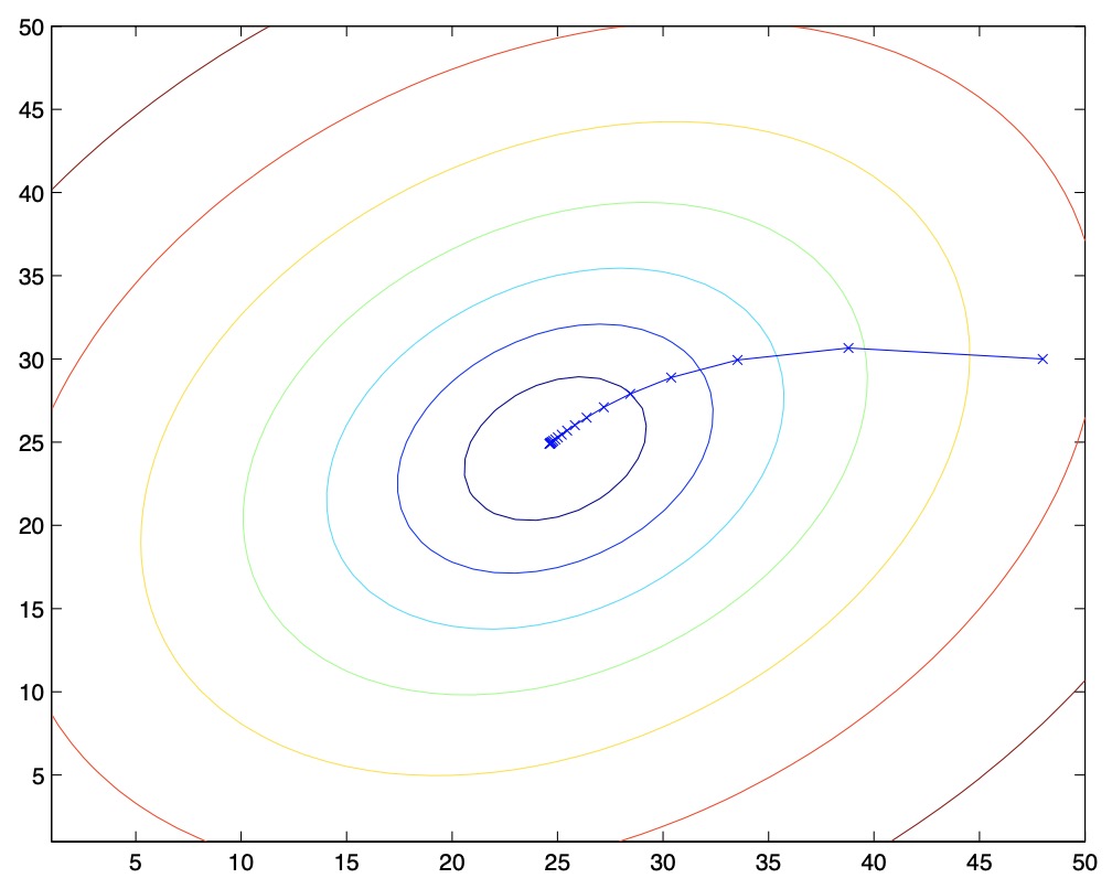
- The ellipses shown above are the contours of a quadratic function. Also shown is the trajectory taken by gradient descent, which was initialized at \((48,30)\). The \(x\)’s in the figure (joined by straight lines) mark the successive values of \(\theta\) that gradient descent went through.
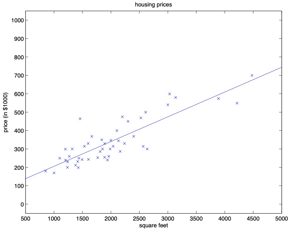
- When we run batch gradient descent to fit \(\theta\) on our previous dataset, to learn to predict housing price as a function of living area, we obtain \(\theta_{0}=71.27, \theta_{1}=0.1345\). If we plot \(h_{\theta}(x)\) as a function of \(x\) (area), along with the training data, we obtain the following figure:
-
If the number of bedrooms were included as one of the input features as well, we get \(\theta_{0}=89.60, \theta_{1}=0.1392, \theta_{2}=-8.738\). The above results were obtained with batch gradient descent. There is an alternative to batch gradient descent that also works very well. Consider the following algorithm:
- for \(i=1\text{ to }\mathrm{m}\):
-
for every \(j\):
\[\theta_{j}:=\theta_{j}+\alpha\left(y^{(i)}-h_{\theta}(x^{(i)})\right) x_{j}^{(i)}\]
-
- for \(i=1\text{ to }\mathrm{m}\):
- In this algorithm, we repeatedly run through the training set, and each time we encounter a training example, we update the parameters according to the gradient of the error with respect to that single training example only. This algorithm is called stochastic gradient descent (also called incremental gradient descent). Whereas batch gradient descent has to scan through the entire training set before taking a single step – a costly operation if \(m\) is large – stochastic gradient descent can start making progress right away, and continues to make progress with each example it looks at.
- Often, stochastic gradient descent gets \(\theta\) “close” to the minimum much faster than batch gradient descent. (Note however that it may never “converge” to the minimum, and the parameters \(\theta\) will keep oscillating around the minimum of \(J(\theta)\); but in practice most of the values near the minimum will be reasonably good approximations to the true minimum. Note that while it is more common to run stochastic gradient descent as we have described it and with a fixed learning rate \(\alpha\), by slowly letting the learning rate \(\alpha\) decrease to zero as the algorithm runs, it is also possible to ensure that the parameters will converge to the global minimum rather then merely oscillate around the minimum.)
- For these reasons, particularly when the training set is large, stochastic gradient descent is often preferred over batch gradient descent.
The normal equations
- Gradient descent gives one way of minimizing \(J(\theta)\). Let’s discuss a second way of doing so, this time performing the minimization explicitly and without resorting to an iterative algorithm. In this method, we will minimize \(J(\theta)\) by explicitly taking its derivatives with respect to the \(\theta_{j}\)’s, and setting them to zero.
- To enable us to do this without having to write reams of algebra and pages full of matrices of derivatives, let’s introduce some notation for doing calculus with matrices.
Matrix derivatives
- For a function \(f: \mathbb{R}^{m \times n} \mapsto \mathbb{R}\) mapping from \(m \times n\) matrices to the real numbers, we define the derivative of \(f\) with respect to \(A\) to be:
- Thus, the gradient \(\nabla_{A} f(A)\) is itself an \(m \times n\) matrix, whose \((i, j)^{th}\) is \(\partial f / \partial A_{i j}\). For example, suppose \(A=\left[\begin{array}{cc}A_{11} & A_{12} \ A_{21} & A_{22}\end{array}\right]\) is a \(2 \times 2\) matrix, and the function \(f: \mathbb{R}^{2 \times 2} \mapsto \mathbb{R}\) is given by,
- Here, \(A_{i j}\) denotes the \((i, j)\) entry of the matrix \(A\).
- We then have,
- We also introduce the trace operator, written \(\text{“tr”}\). For an \(n \times n\) (square) matrix \(A\), the trace of \(A\) is defined to be the sum of its diagonal entries:
-
If \(a\) is a real number (i.e., a \(1 \times 1\) matrix), then \(\text{tr } a=a\). (If you haven’t seen this “operator notation” before, you should think of the trace of \(A\) as \(\operatorname{tr}(A)\), or as application of the “trace” function to the matrix \(A\). It’s more commonly written without the parentheses, however.)
-
The trace operator has the property that for two matrices \(A\) and \(B\) such that \(A B\) is square, we have that \(\operatorname{tr} A B=\operatorname{tr} B A\). As corollaries of this, we also have, e.g.,
- The following properties of the trace operator are also easily verified. Here, \(A\) and \(B\) are square matrices, and \(a\) is a real number:
- We now state without proof some facts of matrix derivatives (we won’t need some of these until later). Equation \((4)\) applies only to non-singular square matrices \(A\), where \(|A|\) denotes the determinant of \(A\). We have:
- To make our matrix notation more concrete, let us now explain in detail the meaning of the first of these equations. Suppose we have some fixed matrix \(B \in \mathbb{R}^{n \times m}\). We can then define a function \(f: \mathbb{R}^{m \times n} \mapsto \mathbb{R}\) according to \(f(A)=\operatorname{tr} A B\). Note that this definition makes sense, because if \(A \in \mathbb{R}^{m \times n}\) then \(A B\) is a square matrix, and we can apply the trace operator to it; thus, \(f\) does indeed map from \(\mathbb{R}^{m \times n}\) to \(\mathbb{R}\).
- We can then apply our definition of matrix derivatives to find \(\nabla_{A} f(A)\), which will itself by an \(m \times n\) matrix. Equation \((1)\) above states that the \((i, j)\) entry of this matrix will be given by the \((i, j)^{th}\) entry of \(B^{T}\), or equivalently, by \(B_{j i}\).
- The proofs of Equations \((1-3)\) are reasonably simple, and are left as an exercise to the reader. Equations \((4)\) can be derived using the adjoint representation of the inverse of a matrix.
- Note that if we define \(A^{\prime}\) to be the matrix whose \((i, j)\) element is \((-1)^{i+j}\) times the determinant of the square matrix resulting from deleting row \(i\) and column \(j\) from \(A\), then it can be proved that \(A^{-1}frac{\left(A^{\prime}\right)^{T}}{|A|}\). (You can check that this is consistent with the standard way of finding \(A^{-1}\) when \(A\) is a \(2 \times 2\) matrix. If you want to see a proof of this more general result, see an intermediate or advanced linear algebra text, such as Charles Curtis, \(1991\), Linear Algebra, Springer.) This shows that \(A^{\prime}=|A|\left(A^{-1}\right)^{T}\). Also, the determinant of a matrix can be written \(|A|=\sum_{j} A_{i j} A_{i j}^{\prime}\). Since \(A_{ij}^{\prime}\) does not depend on \(A_{ij}\) (as can be seen from its definition), this implies that \(\frac{\partial}{\partial A_{i j}} |A|=A_{i j}^{\prime}\). Putting all this together shows the result.
Least squares revisited
- Armed with the tools of matrix derivatives, let us now proceed to find in closed-form the value of \(\theta\) that minimizes \(J(\theta)\). We begin by re-writing \(J(\theta)\) in matrix-vectorial notation.
- Given a training set, define the design matrix \(X\) to be the \(m \times n\) matrix (actually \(m \times n+1\), if we include the intercept term) that contains the training examples’ input values in its rows:
- Also, let \(\vec{y}\) be the \(m\)-dimensional vector containing all the target values from the training set:
- Now, since \(h_{\theta}\left(x^{(i)}\right)=\left(x^{(i)}\right)^{T} \theta\), we can easily verify that,
- Thus, using the fact that for a vector \(z\), we have that \(z^{T} z=\sum_{i} z_{i}^{2}\)
- Finally, to minimize \(J(\theta)\), let’s find its derivatives with respect to \(\theta\). Combining equations \((2)\) and \((3)\), we find that
- Hence,
- In the third step, we used the fact that the trace of a real number is just the real number; the fourth step used the fact that \(\operatorname{tr} A=\operatorname{tr} A^{T}\), and the fifth step used Equation \((5)\) with \(A^{T}=\theta, B=B^{T}=X^{T} X\), and \(C=I\), and Equation \((1)\). To minimize \(J(\theta)\), we set its derivatives to zero, and obtain the normal equations:
- Thus, the value of \(\theta\) that minimizes \(J(\theta)\) is given in closed form by the equation:
Probabilistic interpretation: why squared error?
- When faced with a regression problem, why might linear regression, and specifically least-squares cost function \(J(\theta)\), be a reasonable choice? In this section, we offer a set of probabilistic assumptions, under which least-squares regression fits into place naturally.
-
Let’s use the housing prices problem for this discussion. Assume that the target variable \(y\), which is the true price of every house, is a linear function of the size of the house \(x_1^{(i)}\) and number of bedrooms \(x_2^{(i)}\), plus an error term \(\epsilon^{(i)}\):
\[y^{(i)} = \theta^T x^{(i)}+ \epsilon^{(i)}\]- where \(\epsilon^{(i)}\) is an error term that captures either unmodeled effects (such as features very pertinent to predicting housing price, but that we’d left out of the regression), or random noise.
- Let’s further assume that \(\epsilon^{(i)}\) follows a Gaussian distribution (also called as the Normal distribution) with mean \(\mu = 0\) and variance \(\sigma^2\). Formally,
- This implies that the probability density of \(\epsilon^{(i)}\) follows a Gaussian density function as follows:
- Note that unlike the bell-shaped curve we will see for locally weighted linear regression, this equation does integrate to 1.
- Another assumption we’re going to make is that the \(\epsilon^{(i)}\) error terms are IID, which in statistics stands for independently and identically distributed.
- This implies that the error term for a house is independent of other houses, which might not be a true assumption. For e.g., if one house is priced unusually high, the price on a different house on the same street can probably also be unusually high (owing to say, the school district associated with that area).
- However, the assumption is practical enough to get a pretty good model.
- Under these set of assumptions: (i) \(\epsilon^{(i)}\) follows a Gaussian distribution and, (ii) the \(\epsilon^{(i)}\) error terms are IID, the probability density of \(y^{(i)}\) given \(x^{(i)}\) and \(\theta\) is:
- The notation \(“P(y^{(i)} \mid x^{(i)}; \theta)”\) is read as the probability of \(y^{(i)}\) given \(x^{(i)}\) and parameterized by \(\theta\).
- This implies that \(\theta\) is not a random variable, but is a set of parameters that parameterize the probability distribution denoted by \(P(y^{(i)} \mid x^{(i)}; \theta)\).
- In other words, given x and theta, what’s the probability density of a particular house’s price? It’s a Gaussian with mean \(\mu\) given by \(\theta^T x^{(i)}\), and variance given by \(\sigma^2\). Formally,
- The notation \(“y^{(i)} \mid x^{(i)}; \theta”\) is read as the random variable \(y^{(i)}\) given \(x^{(i)}\) and parameterized by \(\theta\) is sampled from a Gaussian distribution \(\mathcal{N}(\theta^T x^{(i)}, \sigma^2)\).
- We’re essentially modeling the price of a house using the random variable \(y\), as a Gaussian distribution with the mean \(\mu\) as \(\theta^T x^{(i)}\) (i.e., the “true price” of the house), and then accommodating some variation around it by adding noise \(\sigma^2\) to it.
- Given the input features matrix (also called the design matrix) \(X\), which contains all the \(x^{(i)}\)’s and \(\theta\), the probability distribution of \(\vec{y}\), which contains all the \(y^{(i)}\)’s is given by \(P(\vec{y} \mid X; \theta)\). This quantity is typically viewed a function of \(X\), for a fixed value of \(\theta\). When we wish to explicitly view the same quantity as a function of \(\theta\), we instead call it the likelihood function \(L(\cdot)\).
- Formally, the likelikhood of the parameters \(L(\theta)\) is defined as:
- Because we assumed that the errors \(\epsilon^{(i)}\)’s are IID (and hence also the \(y^{(i)}\)’s given the \(x^{(i)}\)’s), the probability of all of the observations in your training set is simply equal to the product of the probabilities:
- Plugging in the definition of \(P(y^{(i)} \mid x^{(i)}; \theta)\) that we had earlier,
- Now, given this probabilistic model relating the \(y^{(i)}\)’s and the \(x^{(i)}\)’s, what is a reasonable way of choosing our best guess of the parameters \(\theta\)? The principal of maximum likelihood says that we should choose \(\theta\) so as to make the data as high probability as possible, i.e., we should choose \(\theta\) to maximize \(L(\theta)\).
- Instead of maximizing \(L(\theta)\), we can also maximize any strictly monotonically increasing function of \(L(\theta)\). In particular, the derivations will be a bit simpler if we instead maximize the log likelihood \(\ell(\theta)\):
- Per the product rule of logarithms, the log of a product is the sum of the logs of its factors, i.e., \(\log{xy} = \log x + \log y\). Applying the log product rule gives us,
- Again, using the product rule of logarithms,
- This simplifies to,
- One of the well-tested methods in statistics for estimating parameters is to use maximum likelihood estimation (MLE) which means you choose \(\theta\) to maximize the likelihood \(L(\theta)\). So given a dataset, an obvious way to choose \(\theta\) is to choose the value that has the highest likelihood. In other words, choose a value of \(\theta\) that maximizes the probability of the data \(P(\vec{y} \mid X; \theta)\).
- Recall that to simplify the derivation, rather than maximizing the likelihood capital \(L(\theta)\), we maximized the log likelihood \(\ell(\theta)\). Since the \(log(\cdot)\) is a strictly monotonically increasing function, the value of \(\theta\) that maximizes the log likelihood should be the same as the value of \(\theta\) that maximizes the likelihood.
- Thus, if you’re using MLE, what you would like to do is choose a value of \(\theta\) that maximizes the equation for \(\ell(\theta)\). But, the first term \(m \log \frac{1}{\sqrt{2 \pi} \sigma}\) is just a constant, since \(\theta\) doesn’t even appear in this term. And so, what you would like to do is choose the value of \(\theta\) that maximizes this second term \(- \frac{1}{2} \sum_{i=1}^{m}\left(y^{(i)}-\theta^{T} x^{(i)}\right)^{2}\). Note that since \(\sigma\) is a constant, i.e., not a function of \(\theta\), the term \(-\frac{1}{\sigma^{2}}\) can be ignored.
- Notice the minus sign in front of the second term. Maximizing the negative of a term is the same as minimizing the term. Hence, maximizing \(\ell(\theta)\) is equivalent to minimizing:
- which we recognize to be \(J(\theta)\), our original least-squares cost function for linear regression.
- This proof shows that choosing the value of \(\theta\) to minimize the least squares error cost function, is equivalent to finding the MLE for the parameters \(\theta\) under the set of assumptions that the error terms \(\epsilon^{(i)}\) are Gaussian and IID.
- Key takeaways
- Under the previous probabilistic assumptions on the data, least-squares regression corresponds to finding the maximum likelihood estimate of \(\theta\).
- This is thus only one set of assumptions under which least-squares regression can be justified as a very natural method that’s just doing maximum likelihood estimation. Note however that the probabilistic assumptions are by no means necessary for least-squares to be a perfectly good and rational procedure, and there may be other natural assumptions that can also be used to justify it.
- Note also that, in our previous discussion, our final choice of \(\theta\) did not depend on what was \(\sigma^2\), and indeed we’d have arrived at the same result even if \(\sigma^2\) were unknown. We will use this fact again later, in our discussion on the exponential family and generalized linear models.
- Under the previous probabilistic assumptions on the data, least-squares regression corresponds to finding the maximum likelihood estimate of \(\theta\).
Rationale for modeling error as a Gaussian
- Most error/noise distributions can be modeled as Gaussian distributions.
- If a distribution is made up of several noise sources which are not too correlated, then we can assume it be a Gaussian using the central limit theorem from statistics.
- For the housing prices problem, the perturbations are: (i) the mood of the seller, (ii) the school district that caters to the area, (iii) the weather in the area or, (iv) access to transportation.
- Given these uncorrelated perturbation sources, adding them up to yield the error terms \(\epsilon^{(i)}\) yields a distribution that can be assumed to be Gaussian.
Likelihood vs. probability
- The likelihood of the parameters \(L(\theta)\) is the same as the probability of the data \(P(\vec{y} \mid X ; \theta)\). However, these exists a subtle difference between the terminology here.
- \(P(\vec{y} \mid X; \theta)\) is a function of the data \(\vec{y} \mid X\) as well as a function of the parameters \(\theta\), depending on which one are you viewing as fixed and which one are you viewing as a variable.
- If you view this quantity as a function of the parameters holding the data fixed, i.e., vary parameters \(\theta\) while keeping the training data \(\vec{y} \mid X\) fixed, we call that the likelihood of the parameters.
- If you view this quantity as a function of the data holding the parameters fixed, i.e., vary data \(\vec{y} \mid X\) while keeping the parameters \(\theta\) fixed, we call that probability of the data.
- Note that \(\theta\) is a set of parameters and is not a random variable.
References
Citation
If you found our work useful, please cite it as:
@article{Chadha2020DistilledLinearRegression,
  title   = {Linear Regression},
  author  = {Chadha, Aman},
  journal = {Distilled Notes for Stanford CS229: Machine Learning},
  year    = {2020},
  note    = {\url{https://aman.ai}}
}