CS229 • Learning Theory
The Bias/Variance Trade-Off
- When talking about linear regression, we discussed the problem of whether to fit a “simple” model such as the linear \(“y=\theta_{0}+\theta_{1} x”\), or a more “complex” model such as the polynomial \(“y=\theta_{0}+\theta_{1} x+\cdots \theta_{5} x^{5}”\). We saw the following example:
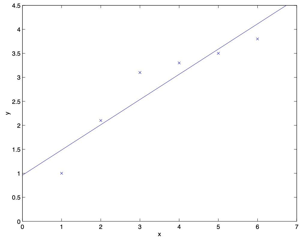
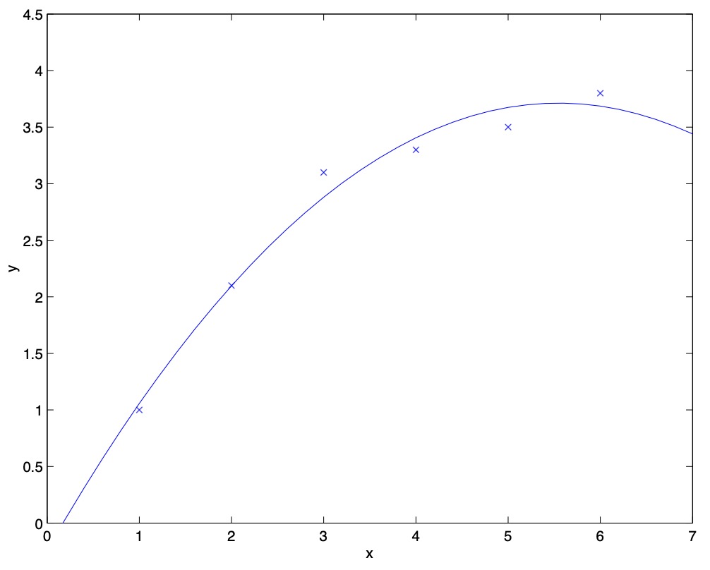
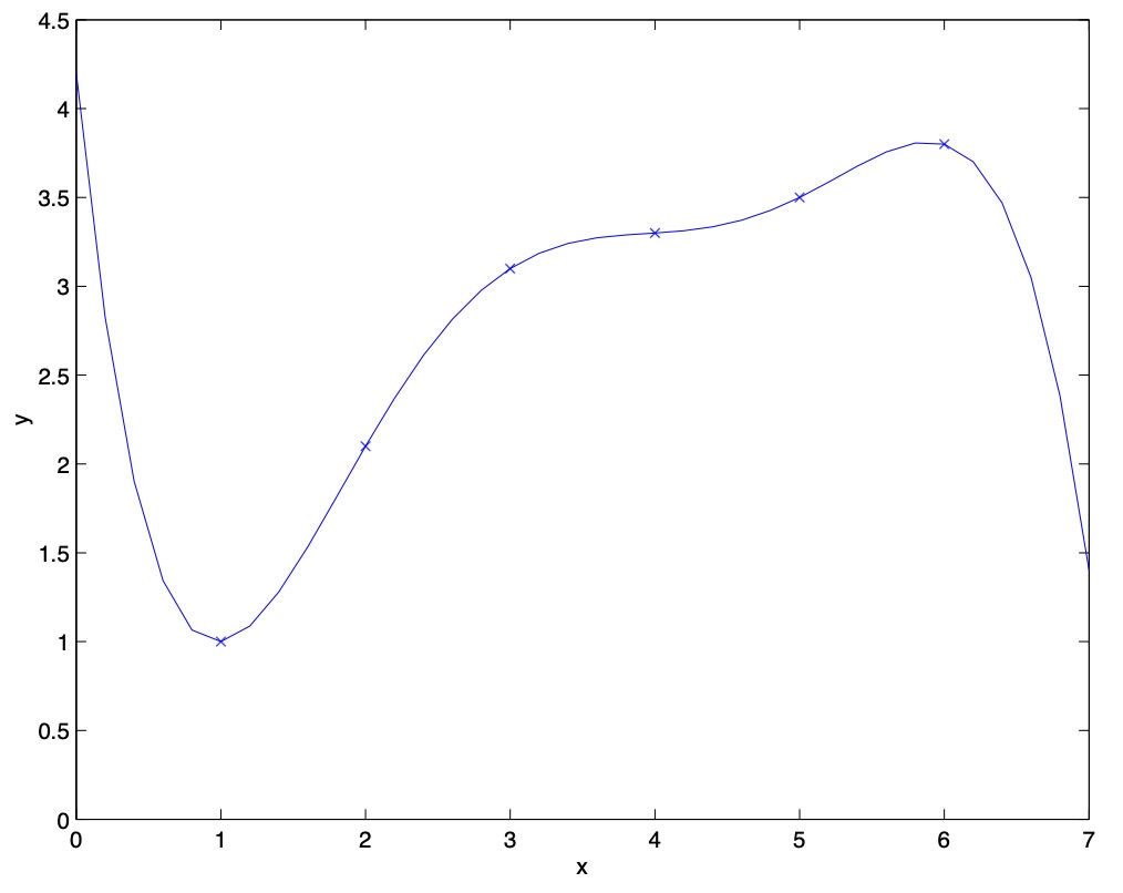
- Fitting a \(5^{th}\) order polynomial to the data (cf. the above figure) did not result in a good model. Specifically, even though the \(5^{th}\) order polynomial did a very good job predicting \(y\) (say, prices of houses) from \(x\) (say, living area) for the examples in the training set, we do not expect the model shown to be a good one for predicting the prices of houses not in the training set.
- In other words, what has been learned from the training set does not generalize well to other houses. The generalization error (which will be made formal shortly) of a hypothesis is its expected error on examples not necessarily in the training set.
- Both the models in the leftmost and the rightmost figures above have large generalization error. However, the problems that the two models suffer from are very different. If the relationship between \(y\) and \(x\) is not linear, then even if we were fitting a linear model to a very large amount of training data, the linear model would still fail to accurately capture the structure in the data.
- Informally, we define the bias of a model to be the expected generalization error even if we were to fit it to a very (say, infinitely) large training set. Thus, for the problem above, the linear model suffers from large bias, and may underfit (i.e., fail to capture structure exhibited by) the data. Apart from bias, there’s a second component to the generalization error, consisting of the variance of a model fitting procedure.
- Specifically, when fitting a \(5^{th}\) order polynomial as in the rightmost figure, there is a large risk that we’re fitting patterns in the data that happened to be present in our small, finite training set, but that do not reflect the wider pattern of the relationship between \(x\) and \(y\). This could be, say, because in the training set we just happened by chance to get a slightly more-expensive-than-average house here, and a slightly less-expensive-than-average house there, and so on. By fitting these “spurious” patterns in the training set, we might again obtain a model with large generalization error. In this case, we say the model has large variance.
- In these notes, we will not try to formalize the definitions of bias and variance beyond this discussion. While bias and variance are straightforward to define formally for, e.g., linear regression, there have been several proposals for the definitions of bias and variance for classification, and there is as yet no agreement on what is the “right” and/or the most useful formalism.
- Often, there is a trade-off between bias and variance. If our model is too “simple” and has very few parameters, then it may have large bias (but small variance); if it is too “complex” and has very many parameters, then it may suffer from large variance (but have smaller bias). In the example above, fitting a quadratic function does better than either of the extremes of a first or a fifth order polynomial.
Preliminaries
- In this section, we begin our foray into learning theory. Apart from being interesting and enlightening in its own right, this discussion will also help us hone our intuitions and derive rules of thumb about how to best apply learning algorithms in different settings. We will also seek to answer a few questions: First, can we make formal the bias/variance trade-off that was just discussed? The will also eventually lead us to talk about model selection methods, which can, for instance, automatically decide what order polynomial to fit to a training set. Second, in machine learning it’s really generalization error that we care about, but most learning algorithms fit their models to the training set. Why should doing well on the training set tell us anything about generalization error? Specifically, can we relate error on the training set to generalization error? Third and finally, are there conditions under which we can actually prove that learning algorithms will work well?
- We start with two simple but very useful lemmas.
- Lemma. The union bound: Let \(A_{1}, A_{2}, \ldots, A_{k}\) be \(k\) different events (that may not be independent). Then,
-
In probability theory, the union bound is usually stated as an axiom (and thus we won’t try to prove it), but it also makes intuitive sense: The probability of any one of \(k\) events happening is at most the sums of the probabilities of the \(k\) different events.
-
Lemma. Hoeffding inequality: Let \(Z_{1}, \ldots, Z_{m}\) be \(m\) independent and identically distributed (iid) random variables drawn from a Bernoulli \((\phi)\) distribution, i.e., \(P\left(Z_{i}=1\right)=\phi\), and \(P\left(Z_{i}=0\right)=1-\phi\). Let \(\hat{\phi}=(1 / m) \sum_{i=1}^{m} Z_{i}\) be the mean of these random variables, and let any \(\gamma>0\) be fixed. Then,
- This lemma (which in learning theory is also called the Chernoff bound) says that if we take \(\hat{\phi}\) the average of \(m\) Bernoulli \((\phi)\) random variables \(-\) to be our estimate of \(\phi\), then the probability of our being far from the true value is small, so long as \(m\) is large. Another way of saying this is that if you have a biased coin whose chance of landing on heads is \(\phi\), then if you toss it \(m\) times and calculate the fraction of times that it came up heads, that will be a good estimate of \(\phi\) with high probability (if \(m\) is large).
-
Using just these two lemmas, we will be able to prove some of the deepest and most important results in learning theory.
-
To simplify our exposition, let’s restrict our attention to binary classification in which the labels are \(y \in\{0,1\}\). Everything we’ll say here generalizes to other, including regression and multi-class classification, problems.
- We assume we are given a training set \(S=\left\{\left(x^{(i)}, y^{(i)}\right) ; i=1, \ldots, m\right\}\) of size \(m\), where the training examples \(\left(x^{(i)}, y^{(i)}\right)\) are drawn iid from some probability distribution \(\mathcal{D}\). For a hypothesis \(h\), we define the training error (also called the empirical risk or empirical error in learning theory) to be
- This is just the fraction of training examples that \(h\) misclassifies. When we want to make explicit the dependence of \(\hat{\varepsilon}(h)\) on the training set \(S\), we may also write this a \(\hat{\varepsilon}_{S}(h)\). We also define the generalization error to be,
-
i.e. this is the probability that, if we now draw a new example \((x, y)\) from the distribution \(\mathcal{D}, h\) will misclassify it.
-
Note that we have assumed that the training data was drawn from the same distribution \(\mathcal{D}\) with which we’re going to evaluate our hypotheses (in the definition of generalization error\). This is sometimes also referred to as one of the PAC assumptions. - PAC stands for “probably approximately correct,” which is a framework and set of assumptions under which numerous results on learning theory were proved. Of these, the assumption of training and testing on the same distribution, and the assumption of the independently drawn training examples, were the most important.
-
Consider the setting of linear classification, and let \(h_{\theta}(x)=1\left\{\theta^{T} x \geq 0\right\}\) What’s a reasonable way of fitting the parameters \(\theta\)? One approach is to try to minimize the training error, and pick
-
We call this process empirical risk minimization (ERM), and the resulting hypothesis output by the learning algorithm is \(\hat{h}=h_{\hat{\theta}}\). We think of ERM as the most “basic” learning algorithm, and it will be this algorithm that we focus on in these notes. (Algorithms such as logistic regression can also be viewed as approximations to empirical risk minimization.)
- In our study of learning theory, it will be useful to abstract away from the specific parameterization of hypotheses and from issues such as whether we’re using a linear classifier. We define the hypothesis class \(\mathcal{H}\) used by a learning algorithm to be the set of all classifiers considered by it. For linear classification, \(\mathcal{H}=\left\{h_{\theta}: h_{\theta}(x)=1\left\{\theta^{T} x \geq 0\right\}, \theta \in \mathbb{R}^{n+1}\right\}\) is thus the set of all classifiers over \(\mathcal{X}\) (the domain of the inputs) where the decision boundary is linear. More broadly, if we were studying, say, neural networks, then we could let \(\mathcal{H}\) be the set of all classifiers representable by some neural network architecture.
- Empirical risk minimization can now be thought of as a minimization over the class of functions \(\mathcal{H}\), in which the learning algorithm picks the hypothesis:
The case of finite \(\mathcal{H}\)
-
Let’s start by considering a learning problem in which we have a finite hypothesis class \(\mathcal{H}=\left\{h_{1}, \ldots, h_{k}\right\}\) consisting of \(k\) hypotheses. Thus, \(\mathcal{H}\) is just a set of \(k\) functions mapping from \(\mathcal{X}\) to \(\{0,1\}\), and empirical risk minimization selects \(\hat{h}\) to be whichever of these \(k\) functions has the smallest training error. We would like to give guarantees on the generalization error of \(\hat{h}\). Our strategy for doing so will be in two parts: First, we will show that \(\hat{\varepsilon}(h)\) is a reliable estimate of \(\varepsilon(h)\) for all \(h\). Second, we will show that this implies an upper-bound on the generalization error of \(\hat{h}\)
-
Take any one, fixed, \(h_{i} \in \mathcal{H}\). Consider a Bernoulli random variable \(Z\) whose distribution is defined as follows. We’re going to sample \((x, y) \sim \mathcal{D}\). Then, we set \(Z=1\left\{h_{i}(x) \neq y\right\}\), i.e., we’re going to draw one example, and let \(Z\) indicate whether \(h_{i}\) misclassifies it. Similarly, we also define \(Z_{j}=\) \(1\left\{h_{i}\left(x^{(j)}\right) \neq y^{(j)}\right\}\). since our training set was drawn iid from \(\mathcal{D}, Z\) and the \(Z_{j}\)’s have the same distribution. We see that the misclassification probability on a randomly drawn example that is, \(\varepsilon(h)-\) is exactly the expected value of \(Z\) (and \(Z_{j}\)). Moreover, the training error can be written
- Thus, \(\hat{\varepsilon}\left(h_{i}\right)\) is exactly the mean of the \(m\) random variables \(Z_{j}\) that are drawn iid from a Bernoulli distribution with mean \(\varepsilon\left(h_{i}\right)\). Hence, we can apply the Hoeffding inequality, and obtain,
- This shows that, for our particular \(h_{i}\), training error will be close to generalization error with high probability, assuming \(m\) is large. But we don’t just want to guarantee that \(\varepsilon\left(h_{i}\right)\) will be close to \(\hat{\varepsilon}\left(h_{i}\right)\) (with high probability) for just only one particular \(h_{i}\). We want to prove that this will be true for simultaneously for all \(h \in \mathcal{H}\). To do so, let \(A_{i}\) denote the event that \(\left|\varepsilon\left(h_{i}\right)-\hat{\varepsilon}\left(h_{i}\right)\right|>\gamma\). We’ve already show that, for any particular \(A_{i}\), it holds true that \(P\left(A_{i}\right) \leq 2 \exp \left(-2 \gamma^{2} m\right)\). Thus, using the union bound, we have,
- If we subtract both sides from 1, we find that,
- The “\neg”symbol means “not”. So, with probability at least \(1-2 k \exp \left(-2 \gamma^{2} m\right)\), we have that \(\varepsilon(h)\) will be within \(\gamma\) of \(\hat{\varepsilon}(h)\) for all \(h \in \mathcal{H}\). This is called a uni form convergence result, because this is a bound that holds simultaneously for all (as opposed to just one) \(h \in \mathcal{H}\).
- In the discussion above, what we did was, for particular values of \(m\) and \(\gamma\), give a bound on the probability that for some \(h \in \mathcal{H},|\varepsilon(h)-\hat{\varepsilon}(h)|>\gamma\). There are three quantities of interest here: \(m, \gamma\), and the probability of error; we can bound either one in terms of the other two.
- For instance, we can ask the following question: Given \(\gamma\) and some \(\delta>0\), how large must \(m\) be before we can guarantee that with probability at least \(1-\delta\), training error will be within \(\gamma\) of generalization error? By setting \(\delta=2 k \exp \left(-2 \gamma^{2} m\right)\) and solving for \(m\), we find that if,
-
then with probability at least \(1-\delta\), we have that \(|\varepsilon(h)-\hat{\varepsilon}(h)| \leq \gamma\) for all \(h \in \mathcal{H}\). (Equivalently, this shows that the probability that \(|\varepsilon(h)-\hat{\varepsilon}(h)|>\gamma\) for some \(h \in \mathcal{H}\) is at most \(\delta\).) This bound tells us how many training examples we need in order make a guarantee. The training set size \(m\) that a certain method or algorithm requires in order to achieve a certain level of performance is also called the algorithm’s sample complexity.
- The key property of the bound above is that the number of training examples needed to make this guarantee is only logarithmic in \(k\), the number of hypotheses in \(\mathcal{H}\}. This will be important later.
- Similarly, we can also hold \(m\) and \(\delta\) fixed and solve for \(\gamma\) in the previous equation, and show that with probability \(1-\delta\), we have that for all \(h \in \mathcal{H}\).
- Now, let’s assume that uniform convergence holds, i.e., that \(|\varepsilon(h)-\hat{\varepsilon}(h)| \leq \gamma\) for all \(h \in \mathcal{H}\). What can we prove about the generalization of our learning algorithm that picked \(\hat{h}=\operatorname*{arg\,min}_{h \in \mathcal{H}} \hat{\varepsilon}(h)\)?
- Define \(h^{\ast}=\operatorname*{arg\,min}_{h \in \mathcal{H}} \varepsilon(h)\) to be the best possible hypothesis in \(\mathcal{H}\). Note that \(h^{\ast}\) is the best that we could possibly do given that we are using \(\mathcal{H}\), so it makes sense to compare our performance to that of \(h^{\ast}\}. We have:
- The first line used the fact that \(|\varepsilon(\hat{h})-\hat{\varepsilon}(\hat{h})| \leq \gamma\) (by our uniform convergence assumption\). The second used the fact that \(\hat{h}\) was chosen to minimize \(\hat{\varepsilon}(h)\) and hence \(\hat{\varepsilon}(\hat{h}) \leq \hat{\varepsilon}(h)\) for all \(h\), and in particular \(\hat{\varepsilon}(\hat{h}) \leq \hat{\varepsilon}\left(h^{\ast}\right)\). The third line used the uniform convergence assumption again, to show that \(\hat{\varepsilon}\left(h^{\ast}\right) \leq\) \(\varepsilon\left(h^{\ast}\right)+\gamma\). So, what we’ve shown is the following: If uniform convergence occurs, then the generalization error of \(\hat{h}\) is at most \(2 \gamma\) worse than the best possible hypothesis in \(\mathcal{H}\)!
- Let’s put all this together into a theorem.
Theorem
- Let \(|\mathcal{H}|=k\), and let any \(m, \delta\) be fixed. Then with probability at least \(1-\delta\), we have,
- This is proved by letting \(\gamma\) equal the \(\sqrt{\cdot}\) term, using our previous argument that uniform convergence occurs with probability at least \(1-\delta\), and then noting that uniform convergence implies \(\varepsilon(h)\) is at most \(2 \gamma\) higher than \(\varepsilon\left(h^{\ast}\right)=\min _{h \in \mathcal{H}} \varepsilon(h)\) (as we showed previously).
- This also quantifies what we were saying previously saying about the bias/variance trade-off in model selection. Specifically, suppose we have some hypothesis class \(\mathcal{H}\), and are considering switching to some much larger hypothesis class \(\mathcal{H}^{\prime} \supseteq \mathcal{H}\). If we switch to \(\mathcal{H}^{\prime}\), then the first term min \(_{h} \varepsilon(h)\) can only decrease (since we’d then be taking a min over a larger set of functions\). Hence, by learning using a larger hypothesis class, our “bias” can only decrease. However, if \(\mathrm{k}\) increases, then the second \(2 \sqrt{\cdot}\) term would also increase. This increase corresponds to our “variance” increasing when we use a larger hypothesis class.
- By holding \(\gamma\) and \(\delta\) fixed and solving for \(m\) like we did before, we can also obtain the following sample complexity bound:
- Corollary. Let \(|\mathcal{H}|=k\), and let any \(\delta, \gamma\) be fixed. Then for \(\varepsilon(\hat{h}) \leq \min _{h \in \mathcal{H}} \varepsilon(h)+2 \gamma\) to hold with probability at least \(1-\delta\), it suffices that,
The case of infinite \(\mathcal{H}\)
-
We have proved some useful theorems for the case of finite hypothesis classes. But many hypothesis classes, including any parameterized by real numbers (as in linear classification) actually contain an infinite number of functions. Can we prove similar results for this setting?
-
Let’s start by going through something that is not the “right” argument. Better and more general arguments exist, but this will be useful for honing our intuitions about the domain.
- Suppose we have an \(\mathcal{H}\) that is parameterized by \(d\) real numbers. since we are using a computer to represent real numbers, and IEEE double-precision floating point (double’s in C) uses 64 bits to represent a floating point number, this means that our learning algorithm, assuming we’re using double-precision floating point, is parameterized by \(64 d\) bits. Thus, our hypothesis class really consists of at most \(k=2^{64 d}\) different hypotheses. From the Corollary at the end of the previous section, we therefore find that, to guarantee \(\varepsilon(\hat{h}) \leq \varepsilon\left(h^{\ast}\right)+2 \gamma\), with to hold with probability at least \(1-\delta\), it suffices that \(m \geq O\left(\frac{1}{\gamma^{2}} \log \frac{2^{64 d}}{\delta}\right)=O\left(\frac{d}{\gamma^{2}} \log \frac{1}{\delta}\right)=O_{\gamma, \delta}(d)\). (The \(\gamma, \delta\) subscripts are to indicate that the last big-\(O\) is hiding constants that may depend on \(\gamma\) and \(\delta\).) Thus, the number of training examples needed is at most linear in the parameters of the model.
- The fact that we relied on 64-bit floating point makes this argument not entirely satisfying, but the conclusion is nonetheless roughly correct: If what we’re going to do is try to minimize training error, then in order to learn “well” using a hypothesis class that has \(d\) parameters, generally we’re going to need on the order of a linear number of training examples in \(d\). (At this point, it’s worth noting that these results were proved for an algorithm that uses empirical risk minimization. Thus, while the linear dependence of sample complexity on \(d\) does generally hold for most discriminative learning algorithms that try to minimize training error or some approximation to training error, these conclusions do not always apply as readily to discriminative learning algorithms. Giving good theoretical guarantees on many non-ERM learning algorithms is still an area of active research.)
- The other part of our previous argument that’s slightly unsatisfying is that it relies on the parameterization of \(\mathcal{H}\). Intuitively, this doesn’t seem like it should matter: We had written the class of linear classifiers as \(h_{\theta}(x)=\) \(1\left\{\theta_{0}+\theta_{1} x_{1}+\cdots \theta_{n} x_{n} \geq 0\right\}\), with \(n+1\) parameters \(\theta_{0}, \ldots, \theta_{n}\). But it could also be written \(h_{u, v}(x)=1\left\{\left(u_{0}^{2}-v_{0}^{2}\right)+\left(u_{1}^{2}-v_{1}^{2}\right) x_{1}+\cdots\left(u_{n}^{2}-v_{n}^{2}\right) x_{n} \geq 0\right\}\) with \(2 n+2\) parameters \(u_{i}, v_{i}\). Yet, both of these are just defining the same \(\mathcal{H}:\) The set of linear classifiers in \(n\) dimensions.
- To derive a more satisfying argument, let’s define a few more things. Given a set \(S=\left\{x^{(i)}, \ldots, x^{(d)}\right\}\) (no relation to the training set) of points \(x^{(i)} \in \mathcal{X}\), we say that \(\mathcal{H}\) shatters \(S\) if \(\mathcal{H}\) can realize any labeling on \(S\), i.e., if for any set of labels \(\left\{y^{(1)}, \ldots, y^{(d)}\right\}\), there exists some \(h \in \mathcal{H}\) so that \(h\left(x^{(i)}\right)=y^{(i)}\) for all \(i=1, \ldots, d\).
- Given a hypothesis class \(\mathcal{H}\), we then define its Vapnik-Chervonenkis dimension, written \(\mathrm{VC}(\mathcal{H})\), to be the size of the largest set that is shattered by \(\mathcal{H}\). (If \(\mathcal{H}\) can shatter arbitrarily large sets, then \(\mathrm{VC}(\mathcal{H})=\infty\).)
- For instance, consider the following set of three points:
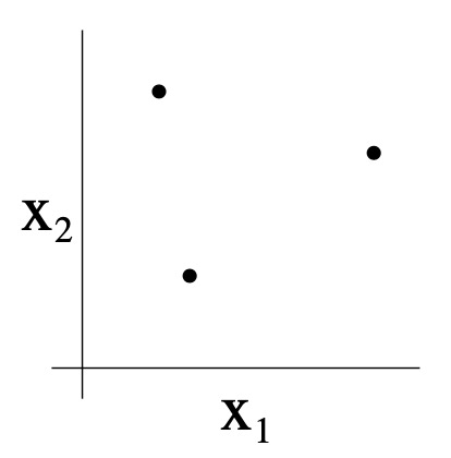
- Can the set \(\mathcal{H}\) of linear classifiers in two dimensions \(\left(h(x)=1\left\{\theta_{0}+\theta_{1} x_{1}+\right\}\right)\). \(\left.\theta_{2} x_{2} \geq 0\right\}\)) can shatter the set above? The answer is yes. Specifically, we see that, for any of the eight possible labelings of these points, we can find a linear classifier that obtains “zero training error” on them:
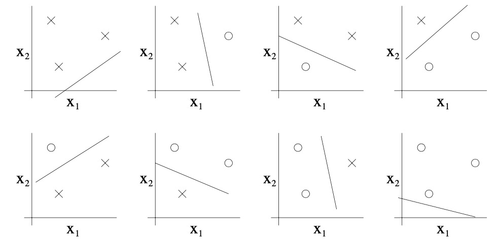
- Moreover, it is possible to show that there is no set of 4 points that this hypothesis class can shatter. Thus, the largest set that \(\mathcal{H}\) can shatter is of size 3, and hence \(\mathrm{VC}(\mathcal{H})=3\).
- Note that the VC dimension of \(\mathcal{H}\) here is 3 even though there may be sets of size 3 that it cannot shatter. For instance, if we had a set of three points lying in a straight line (left figure), then there is no way to find a linear separator for the labeling of the three points shown below (right figure):
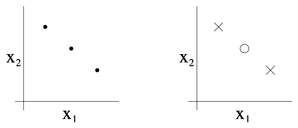
- In order words, under the definition of the VC dimension, in order to prove that \(\operatorname{VC}(\mathcal{H})\) is at least \(d\), we need to show only that there’s at least one set of size \(d\) that \(\mathcal{H}\) can shatter.
- The following theorem, due to Vapnik, can then be shown. (This is, many would argue, the most important theorem in all of learning theory.)
- Theorem. Let \(\mathcal{H}\) be given, and let \(d=\mathrm{VC}(\mathcal{H})\). Then with probability at least \(1-\delta\), we have that for all \(h \in \mathcal{H}\).
- Thus, with probability at least \(1-\delta\), we also have that:
- In other words, if a hypothesis class has finite VC dimension, then uniform convergence occurs as \(m\) becomes large. As before, this allows us to give a bound on \(\varepsilon(h)\) in terms of \(\varepsilon\left(h^{\ast}\right)\). We also have the following corollary:
- Corollary. For \(|\varepsilon(h)-\hat{\varepsilon}(h)| \leq \gamma\) to hold for all \(h \in \mathcal{H}\) (and hence \(\varepsilon(\hat{h}) \leq \left.\varepsilon\left(h^{\ast}\right)+2 \gamma\right)\) with probability at least \(1-\delta\), it suffices that \(m=O_{\gamma, \delta}(d)\). In other words, the number of training examples needed to learn “well” using \(\mathcal{H}\) is linear in the VC dimension of \(\mathcal{H}\). It turns out that, for “most” hypothesis classes, the VC dimension (assuming a “reasonable” parameterization) is also roughly linear in the number of parameters. Putting these together, we conclude that (for an algorithm that tries to minimize training error) the number of training examples needed is usually roughly linear in the number of parameters of \(\mathcal{H}\).
References
- CS229 Notes.
- “Reconciling modern machine learning and the bias-variance trade-off” (2019) by Nakkiran et al. presents an in-depth treatment on deep double descent.
- Deep Double Descent for the overview of the paper.
- Daniela Witten’s Twitter for the awesome double descent explanation.
- “Reconciling modern machine learning and the bias-variance trade-off” (2018) by Belkin et al. is actually the original “double descent” paper.
- Yannic Kilcher’s YouTube video presents a nice visual walkthrough of the paper.
Citation
If you found our work useful, please cite it as:
@article{Chadha2020DistilledLearningTheory,
  title   = {Learning Theory},
  author  = {Chadha, Aman},
  journal = {Distilled Notes for Stanford CS229: Machine Learning},
  year    = {2020},
  note    = {\url{https://aman.ai}}
}