Aman's AI Journal • Video Recommendation

Problem statement

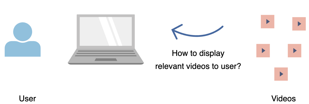
Build a video recommendation system for YouTube users. We want to maximize users’ engagement and recommend new types of content to users.

Metrics
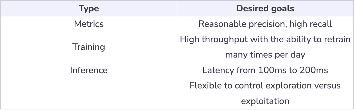
- Offline metrics: Use precision, recall, ranking loss, and logloss.
- Online metrics: Use A/B testing to compare Click Through Rates, watch time, and Conversion rates.
Requirements
- Training
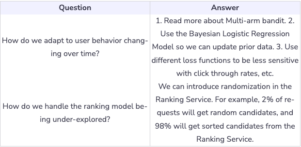
  - User behavior is generally unpredictable, and videos can become viral during the day. Ideally, we want to train many times during the day to capture temporal changes.
Inference
- For every user to visit the homepage, the system will have to recommend 100 videos for them. The latency needs to be under 200ms, ideally sub 100ms.
- For online recommendations, it’s important to find the balance between exploration vs. exploitation. If the model over-exploits historical data, new videos might not get exposed to users. We want to balance between relevancy and fresh new content.

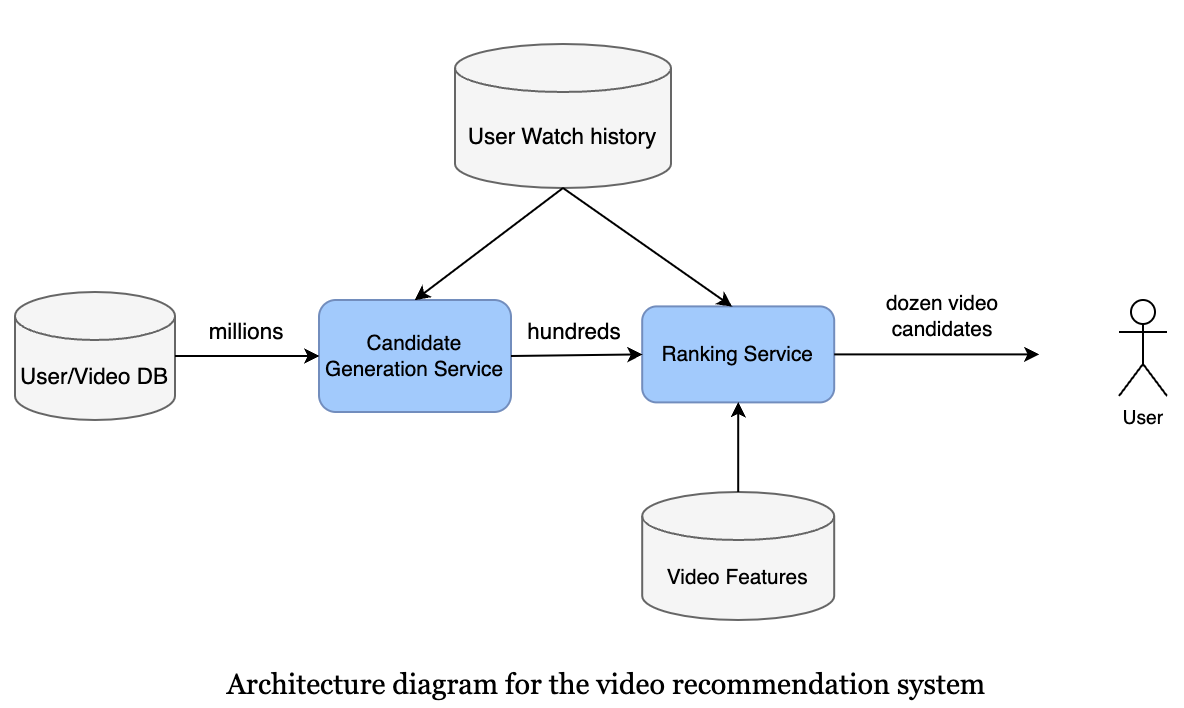
There are two stages, candidate generation, and ranking. The reason for two stages is to make the system scale.
It’s a common pattern that you will see in many ML systems.
We will explore the two stages in the section below.
The candidate model will find the relevant videos based on user watch history and the type of videos the user has watched.
The ranking model will optimize for the view likelihood, i.e., videos that have high a watch possibility should be ranked high. It’s a natural fit for the logistic regression algorithm.

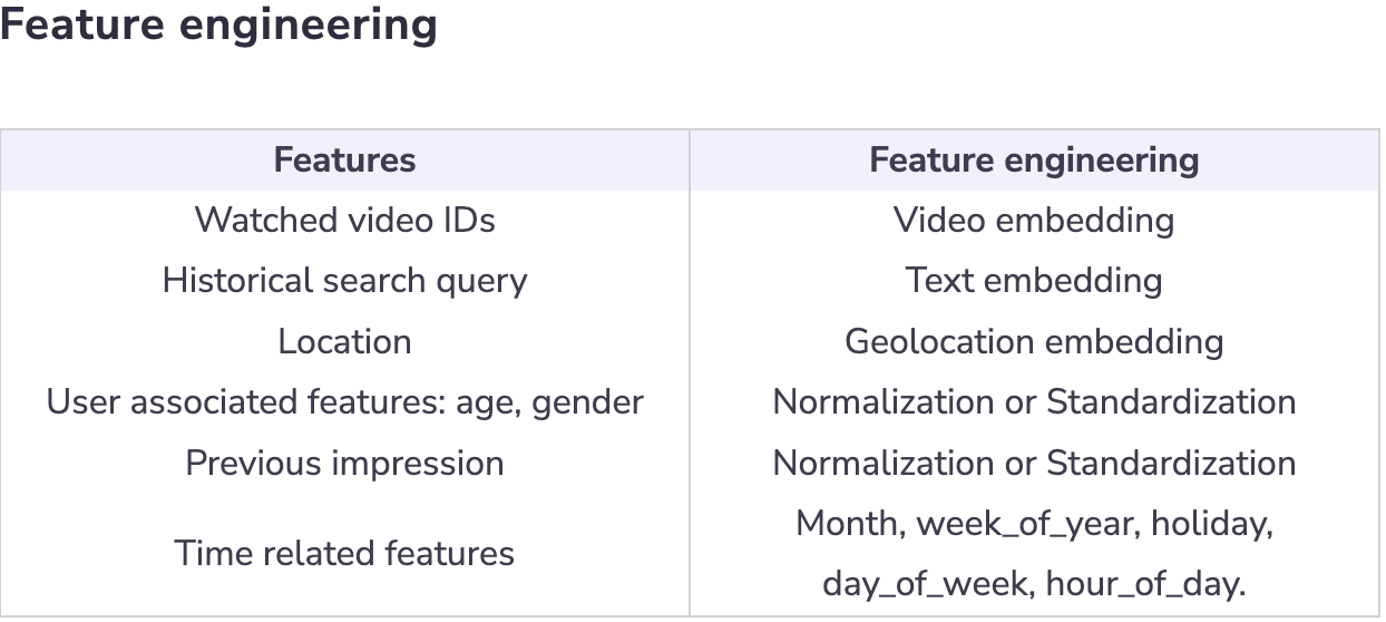
Feature engineering
- Each user has a list of video watches (videos, minutes_watched).
Training data
- For generating training data, we can make a user-video watch space. We can start by selecting a period of data like last month, last 6 months, etc. This should find a balance between training time and model accuracy.
Model
- The candidate generation can be done by Matrix factorization. The purpose of candidate generation is to generate “somewhat” relevant content to users based on their watched history. The candidate list needs to be big enough to capture potential matches for the model to perform well with desired latency.
- One solution is to use collaborative algorithms because the inference time is fast, and it can capture the similarity between user taste in the user-video space.
In practice, for large scale system (Facebook, Google), we don’t use Collaborative Filtering and prefer low latency method to get candidate. One example is to leverage Inverted Index (commonly used in Lucene, Elastic Search). Another powerful technique can be found FAISS or Google ScaNN.

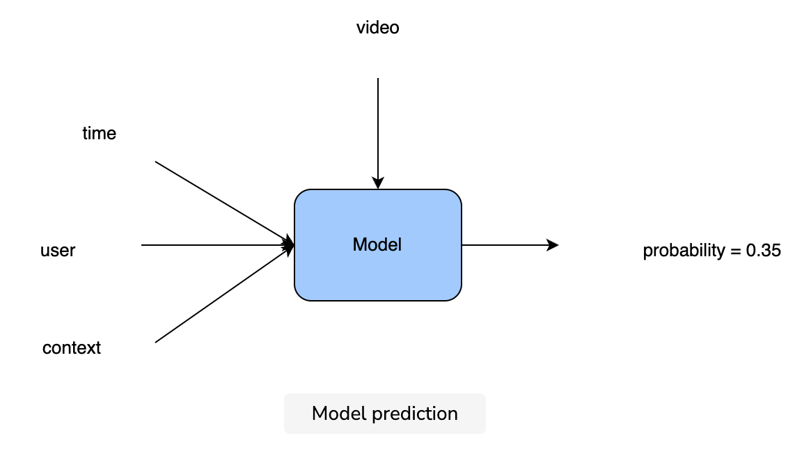
During inference, the ranking model receives a list of video candidates given by the Candidate Generation model. For each candidate, the ranking model estimates the probability of that video being watched. It then sorts the video candidates based on that probability and returns the list to the upstream process.

We can use User Watched History data. Normally, the ratio between watched vs. not-watched is 2/98. So, for the majority of the time, the user does not watch a video.
Model
- At the beginning, it’s important that we started with a simple model, as we can add complexity later.
- A fully connected neural network is simple yet powerful for representing non-linear relationships, and it can handle big data.
- We start with a fully connected neural network with sigmoid activation at the last layer. The reason for this is that the Sigmoid function returns value in the range [0, 1]; therefore it’s a natural fit for estimating probability.
For deep learning architecture, we can use relu, (Rectified Linear Unit), as an activation function for hidden layers. It’s very effective in practice.
The loss function can be cross-entropy loss.

For 1 month, we collected 15 billion positive labels and 750 billion negative labels.
Generally, we can assume that for every data point we collect, we also collect hundreds of features. For simplicity, each row takes 500 bytes to store. In one month, we need 800 billion rows. Total size: \(500 * 800 * 10^9=4 * 10^{14} \text { bytes }=0.4\) Petabytes.
To save costs, we can keep the last six months or one year of data in the data lake, and archive old data in cold storage.

Assume that every second we have to generate a recommendation request for 10 million users. Each request will generate ranks for 1k-10k videos.

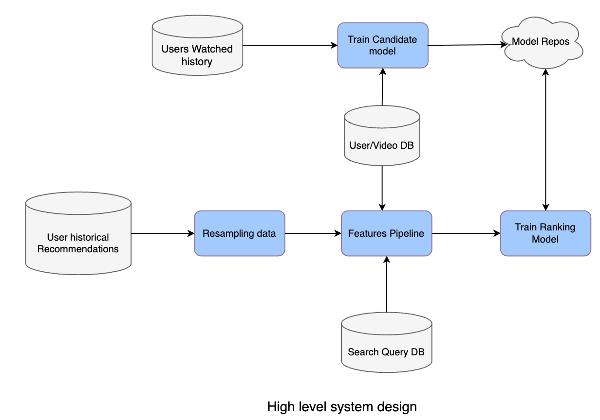
Database
- User Watched history stores which videos are watched by a particular user overtime.
- Search Query DB stores ahistorical queries that users have searched in the past. User/Video DB stores a list of Users and their profiles along with Video metadata.
- User historical recommendations stores past recommendations for a particular user.
- Resampling data: It’s part of the pipeline to help scale the training process by down-sampling negative samples.
Feature pipeline: A pipeline program to generate all required features for training a model. It’s important for feature pipelines to provide high throughput, as we require this to retrain models multiple times. We can use Spark or Elastic MapReduce or Google DataProc.
Model Repos: Storage to store all models, using AWS S3 is a popular option.
In practice, during inference, it’s desirable to be able to get the latest model near real-time. One common pattern for the inference component is to frequently pull the latest models from Model Repos based on timestamp.

Huge data size
- Solution: Pick 1 month or 6 months of recent data.
Imbalance data
- Solution: Perform random negative down-sampling.
High availability
- Solution 1: Use model-as-a-service, each model will run in Docker containers.
- Solution 2: We can use Kubernetes to auto-scale the number of pods.
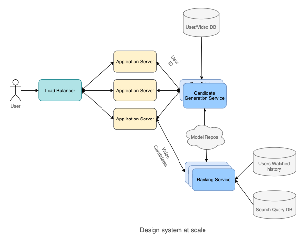
Let’s examine the flow of the system:

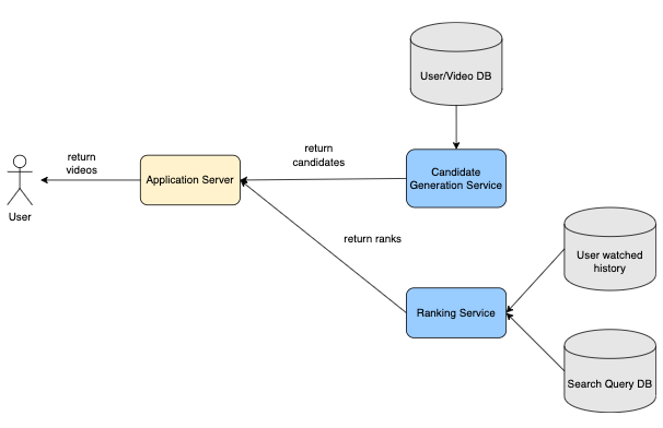
When a user requests a video recommendation, the Application Server requests Video candidates from the Candidate Generation Model. Once it receives the candidates, it then passes the candidate list to the ranking model to get the sorting order. The ranking model estimates the watch probability and returns the sorted list to the Application Server.
The Application Server then returns the top videos that the user should watch.

Scale out (horizontal) multiple Application Servers and use Load Balancers to balance loads.
Scale out (horizontal) multiple Candidate Generation Services and Ranking Services.
It’s common to deploy these services in a Kubernetes Pod and take advantage of the Kubernetes Pod Autoscaler to scale out these services automatically.
In practice, we can also use Kube-proxy so the Candidate Generation Service can call Ranking Service directly, reducing latency even further.