Recommendation Systems • System Design
- Overview
- Glossary
- Cheat Sheet
- Components Cheatsheet
- Rate limiters
- Monitoring systems
- SQL vs NoSQL
- Blob storage
- Key value stores
- Load balancer
- Kafka
- Streaming Platform:
- Streaming Platform:
- Real-Time Stream Processing:
- Serverless Computing (Task Runners):
- Data Storage (Click Capture, Aggregated Data):
- Content Delivery Network (CDN):
- Analytics Service:
- MapReduce for Reconciliation:
- Caching Systems:
- Non-Relational Databases (NoSQL):
- Relational Databases (SQL):
- Columnar Databases:
- Parquet (Columnar File Format):
- Summary:
- System Design Cheatsheet
- Basic Steps
- Key topics for designing a system
- Web App System design considerations:
- Working Components of Front-end Architecture
- Embeddings
- Hashing trick
- Facebook Ads Ranking
- Twitter’s Recommendation Algorithm
- Twitter’s Retrieval Algorithm: Deep Retrieval
- TikTok Recommender System
- Collisionless hashing
- Dynamic size embeddings
- Instantaneous updates during runtime
- Sparse variables:
- Conflated categories:
- Candidate generation stage
- Fine ranking stage
- Multi-gate Mixture of Experts
- Correcting selection bias
- Sampling the data for Offline training
- Real time streaming engine for online training
- Streaming engine architecture
- Google Search - by Damien Benveniste, PHD
- Overview of current systems from Eugene Yan
- Alibab
- JD
- DoorDash
- Batch vs Real- time
- Fresh Content Needs More Attention: Multi-funnel Fresh Content Recommendation
Overview
- On this page we will look at the different types of recommender systems out there and focus on their system’s design.
- Specifically, we will delve deeper into the machine learning architecture and algorithms that make up these systems.
- Recommender systems usually follow a similar, multi-stage pattern of a candidate generation stage, retrieving, and ranking. The real magic is in how each of these steps are implemented.
- Some common vector embedding methods include: matrix factorization (MF), factorization machines (FM), DeepFM, and Field-aware FM (FFM).
- Recommender systems can be used to solve a variety of prediction problems, including:
- Rating prediction: In this problem, the goal is to predict the rating that a user will give to an item on a numerical scale, such as a 5-star rating system.
- Top-N recommendation: In this problem, the goal is to recommend a ranked list of N items to a user, based on their preferences and past interactions.
- Next item recommendation: In this problem, the goal is to recommend the next item that a user is likely to interact with, based on their current context and past interactions.
Glossary
Parquet- A Column-Oriented Data Format
- Apache Parquet is an open-source, columnar data file format designed for efficient storage and retrieval.
- Organizing data by column enhances compression, speeds analytics, and supports complex structures.
- Parquet’s benefits include space savings, faster queries, and compatibility with advanced nested data types, making it particularly effective for analytics tasks, as opposed to row-based formats like CSV.
- It’s a popular choice for interactive and serverless technologies such as AWS Athena and Google BigQuery, bringing efficiency and cost savings to large datasets.
Optimized Row Columnar (ORC) Format for Advertising Data
- The Optimized Row Columnar (ORC) file format, integrated with Apache Hive, excels in efficiently storing and analyzing large datasets, particularly for advertising purposes within the Hadoop ecosystem.
- ORC’s advantages include storage of extensive advertising data, rapid performance analysis, effective targeting, fraud detection, historical trend analysis, integration with various systems, scalability, and more, making it a crucial asset for modern advertising infrastructure platforms.
OLAP
- OLAP: OLAP functions enable the analysis of multidimensional data, which can be crucial in a context like advertising, where you want to understand user behavior, campaign performance, etc., across various dimensions like time, geography, demography, and so on.
- OLAP capabilities are most commonly associated with databases that support analytical processing, although some of the mentioned functions or their equivalents are available in various RDBMS (Relational Database Management Systems) as well.
- MySQL:
- MySQL, especially in its earlier versions, did not have robust OLAP functions. But over time, it has added window functions (starting from MySQL 8.0) similar to those in other databases. Functions like
RANK(),LEAD(),LAG(), and moving averages using window functions are supported. - Example:
SELECT advertiser, impressions,
       RANK() OVER(PARTITION BY advertiser ORDER BY impressions DESC) as rank
FROM ad_data;
- MySQL, especially in its earlier versions, did not have robust OLAP functions. But over time, it has added window functions (starting from MySQL 8.0) similar to those in other databases. Functions like
- PostgreSQL:
- PostgreSQL has a more extensive set of OLAP functions compared to earlier versions of MySQL. It supports window functions and CTEs (Common Table Expressions) which can be used to create more complex OLAP-style queries.
- Example:
WITH MonthlySpend AS (
    SELECT date_trunc('month', ad_date) as month, SUM(spend) as total_spend
    FROM ad_data
    GROUP BY date_trunc('month', ad_date)
)
SELECT month, total_spend,
       LAG(total_spend) OVER(ORDER BY month) as last_month_spend
FROM MonthlySpend;
- Oracle:
- Oracle has robust OLAP capabilities with a wide variety of OLAP and analytic functions. Functions like
ROLLUP,CUBE, and others are natively supported. - Example:
SELECT advertiser, SUM(impressions) as total_impressions
FROM ad_data
GROUP BY ROLLUP(advertiser);
- Oracle has robust OLAP capabilities with a wide variety of OLAP and analytic functions. Functions like
- SQL Server:
- SQL Server also has strong OLAP features and supports CTEs, window functions, and the
PIVOToperation which can be used for some OLAP-style queries. - Example:
SELECT advertiser, SUM(clicks) as total_clicks
FROM ad_data
GROUP BY GROUPING SETS(advertiser, ad_date);
- SQL Server also has strong OLAP features and supports CTEs, window functions, and the
- Databases designed explicitly for OLAP operations, like Microsoft Analysis Services, Oracle OLAP, or IBM Cognos, have even more advanced analytical capabilities, often with their own specialized query languages.
- Most of these functions are used in relational databases, but their implementation and exact syntax might vary across different databases. If you are considering using these functions, always consult the specific documentation for your RDBMS to ensure you’re using the correct syntax and to understand any limitations or specifics of that system.
Cheat Sheet
Components Cheatsheet
Rate limiters
- A rate limiter sets a limit for the number of requests a service will fulfill. It will throttle requests that cross this threshold.
- Rate limiters are an important line of defense for services and systems. They prevent services from being flooded with requests. By disallowing excessive requests, they can mitigate resource consumption.
Monitoring systems
- Monitoring systems are software that allow system administrators to monitor infrastructure. This building block of system design is important because it creates one centralized location for observing the overall performance of a potentially large system of computers in real time.
- Monitoring systems should have the ability to monitor factors such as:
- CPUs
- Server memory
- Routers
- Switches
- Bandwidth
- Applications
- Performance and availability of important network devices
SQL vs NoSQL
- When to pick a SQL database?
- If you are writing a stock trading, banking, or a Finance-based app or you need to store a lot of relationships, for instance, when writing a social networking app like Facebook, then you should pick a relational database. Here’s why:
- Transactions & Data Consistency
- If you are writing software that has anything to do with money or numbers, that makes transactions, ACID, data consistency super important to you. Relational DBs shine when it comes to transactions & data consistency. They comply with the ACID rule, have been around for ages & are battle-tested.
- Storing Relationships
- If your data has a lot of relationships like “friends in Seattle”, “friends who like coding” etc. There is nothing better than a relational database for storing this kind of data.
- Relational databases are built to store relationships. They have been tried & tested & are used by big guns in the industry like Facebook as the main user-facing database.
- Popular relational databases:
- MySQL
- Microsoft SQL Server
- PostgreSQL
- MariaDB
- When to pick a NoSQL database
- Here are a few reasons why you’d want to pick a NoSQL database:
- Handling A Large Number Of Read Write Operations
- Look towards NoSQL databases when you need to scale fast. For example, when there are a large number of read-write operations on your website and when dealing with a large amount of data, NoSQL databases fit best in these scenarios. Since they have the ability to add nodes on the fly, they can handle more concurrent traffic and large amounts of data with minimal latency.
- Running data analytics NoSQL databases also fit best for data analytics use cases, where we have to deal with an influx of massive amounts of data.
- Popular NoSQL databases:
- MongoDB
- Redis
- Cassandra
- HBASE
Blob storage
- Blob, or binary large object, storage is a storage solution for unstructured data. This data can be mostly any type: photos, audio, multimedia, executable code, etc.
- Blob storage uses flat data organization patterns, meaning there is no hierarchy of directories or sub-directories.
- Most blob storage services such as Microsoft Azure or AWS S3 are built around a rule that states “write once, read many” or WORM. This ensures that important data is protected since once the data is written it can be read but not changed.
- Blob stores are ideal for any application that is data heavy. Some of the most notable users of blob stores are:
- YouTube (Google Cloud Storage)
- Netflix (Amazon S3)
- Facebook (Tectonic)
- These services generate enormous amounts of data through large media files. It is estimated that YouTube alone generates a petabyte (1024 terabytes!) of data every day.
Key value stores
- A key value store or key value database are storage systems similar to hash tables or dictionaries. Hash tables and dictionaries are associative as they store information as a pair in the (key, value) format. Information can easily be retrieved and sorted as a result of every value being linked to a key.
- Key value stores are distributed hash tables (DHT).
- Distributed hash tables are just decentralized versions of hash tables. This means they share the key-value pair and lookup methods.
- The keys in a key value store treat data as a single opaque collection. The stored data could be a blob, server name, image, or anything the user wants to store. The values are referred to as opaque data types since they are effectively hidden by their method of storage. It is important that data types are opaque in order to support concepts like information hiding and object-oriented programming (OOP).
- Examples of contemporary, large-scale key value stores are Amazon’s DynamoDB and Microsoft Cassandra.
Load balancer
- Load balancing is a key building block of system design. It involves delegating tasks over a set width of resources.
- There may be millions of requests per second to a system on average. Load balancers ensure that all of these requests can be processed by dividing them between available servers.
- This way, the servers will have a more manageable stream of tasks, and it is less likely that one server will be overburdened with requests. Evenly distributing the computational load allows for faster response times and the capacity for more web traffic.
- Load balancers are a crucial part of the system design process. They enable several key properties required for modern web design.
- Scaling: Load balancers facilitate scaling, either up or down, by disguising changes made to the number of servers.
- Availability: By dividing requests, load balancers maintain availability of the system even in the event of a server outage.
- Performance: Directing requests to servers with low traffic decreases response time for the end user.
Kafka
- Apache Kafka as a Streaming Platform:
- While Kafka does function as a messaging system, it goes beyond simple message queuing by providing features that are crucial for handling real-time data streams, making it suitable for use as a streaming platform:
- Event Storage: Kafka retains data for a specified time period, allowing applications to consume data at their own pace. This feature is crucial for building historical data pipelines.
- Scalability: Kafka is designed to handle high throughput and can be scaled horizontally across multiple nodes or clusters, making it suitable for large-scale streaming scenarios.
- Fault Tolerance: Kafka replicates data across multiple brokers, ensuring data availability even in the face of hardware failures.
- Event Time Processing: Kafka supports event-time processing, which is a key requirement for many streaming use cases, such as windowed aggregations and accurate time-based analytics.
- Exactly-Once Processing: Kafka introduced support for exactly-once message processing, ensuring that events are neither lost nor duplicated during processing.
- Streams API: Kafka provides the Kafka Streams API, which enables developers to build complex streaming applications, including transformations, joins, and aggregations.
- Integration with Ecosystem: Kafka integrates well with other big data and streaming tools, allowing data to be ingested from various sources and consumed by different processing engines.
Streaming Platform:
Certainly, and I’ll incorporate Apache Flink into the explanation of streaming platforms:
Streaming Platform:
- A streaming platform is a software framework designed to process and analyze continuous streams of data in real-time.
-
It enables organizations to ingest, process, and respond to data as it arrives, allowing for timely insights and actions. Here are a few popular streaming platforms:
- Apache Kafka:
- Advantages: High throughput, scalable, fault-tolerant, and capable of handling millions of events per second.
- Disadvantages: Complex to set up and manage, requires tuning for optimal performance.
- Amazon Kinesis:
- Advantages: Fully managed, integrates well with AWS ecosystem, good scalability.
- Disadvantages: Less flexibility compared to Kafka, potentially higher costs.
- Apache Kafka:
-
Streaming Analytics Framework:
- Apache Flink:
- Advantages: A powerful open-source stream processing framework that supports both batch and stream processing, providing event-time processing, fault tolerance, and state management.
- Disadvantages: Requires more understanding of stream processing concepts, may have a steeper learning curve compared to simpler stream processing tools.
- Apache Flink:
Explanation:
-
Streaming platforms, such as Apache Kafka and Amazon Kinesis, serve as infrastructure for handling real-time data. They offer capabilities to ingest data, manage it, and distribute it to various consumers or processing pipelines.
-
Streaming Analytics Frameworks, like Apache Flink, extend the functionality of streaming platforms by allowing data processing, transformations, and complex analytics on the incoming data streams. These frameworks enable real-time data analysis and insights extraction.
-
In summary, streaming platforms and streaming analytics frameworks collectively empower organizations to harness the power of real-time data, making it possible to react swiftly to events, make informed decisions, and provide dynamic services based on the most up-to-date information.
Real-Time Stream Processing:
- Apache Flink:
- Advantages: Low latency, exactly-once processing semantics, strong community support.
- Disadvantages: Can be complex to configure, high resource consumption.
- Apache Storm:
- Advantages: Low-latency processing, scalable, reliable.
- Disadvantages: Lacks native exactly-once processing, older and losing community support.
Serverless Computing (Task Runners):
- AWS Lambda:
- Advantages: Fully managed, scales automatically, pay-per-use pricing.
- Disadvantages: Cold starts can add latency, limitations on execution time and resources.
- Azure Functions:
- Advantages: Integrates well with Microsoft products, flexible pricing, multiple language support.
- Disadvantages: Cold starts, less mature than AWS Lambda.
Data Storage (Click Capture, Aggregated Data):
- Amazon Redshift:
- Advantages: Fully managed, excellent for analytics, integrates with AWS.
- Disadvantages: Can be expensive, less suitable for unstructured data.
- Apache Cassandra:
- Advantages: Highly scalable, fault-tolerant, good for write-heavy workloads.
- Disadvantages: Complex to manage, potential consistency issues.
Content Delivery Network (CDN):
- Amazon CloudFront:
- Advantages: Integrates with other AWS services, global reach, good performance.
- Disadvantages: Costs can escalate, less flexibility in certain configurations.
- Cloudflare:
- Advantages: Strong security features, broad network, performance optimization features.
- Disadvantages: Some configurations can be complex, potential issues with specific ISPs.
Analytics Service:
- Tableau:
- Advantages: User-friendly, powerful visualization capabilities.
- Disadvantages: Can be expensive, heavy resource consumption.
- Power BI:
- Advantages: Integrates well with Microsoft products, robust reporting capabilities.
- Disadvantages: Less flexible with non-Microsoft products, licensing costs.
MapReduce for Reconciliation:
- Apache Hadoop:
- Advantages: Scalable, robust, well-suited for batch processing.
- Disadvantages: Complex to set up and manage, not suited for real-time processing.
- Apache Spark:
- Advantages: Faster than Hadoop, can handle real-time processing, supports various languages.
- Disadvantages: Requires substantial resources, can be complex to optimize.
Caching Systems:
- Redis:
- Advantages: High-performance, in-memory data store, supports various data structures, persistent.
- Disadvantages: Limited to available RAM, cluster mode can add complexity.
- Memcached:
- Advantages: Easy to use, fast, in-memory key-value store, suitable for simple caching needs.
- Disadvantages: No persistence, less versatile than Redis.
Non-Relational Databases (NoSQL):
- MongoDB:
- Advantages: Flexible schema, horizontal scalability, good for unstructured data.
- Disadvantages: Potential consistency issues, less suited for complex transactions.
- Apache Cassandra:
- Advantages: Write-optimized, highly scalable, distributed.
- Disadvantages: Read latency can be high, complex to manage.
Relational Databases (SQL):
- MySQL:
- Advantages: Well-established, wide community support, ACID compliant.
- Disadvantages: Scalability limitations, can struggle with very large datasets.
- PostgreSQL:
- Advantages: Extensible, strong consistency, robust feature set.
- Disadvantages: Can be resource-intensive, less suitable for write-heavy loads.
Columnar Databases:
- Amazon Redshift:
- Advantages: Optimized for analytics, compresses well, integrates with AWS ecosystem.
- Disadvantages: Less suited for transactional workloads, can be expensive.
- Apache HBase:
- Advantages: Scalable, good for real-time read/write access.
- Disadvantages: Complexity in management, consistency can be a challenge.
Parquet (Columnar File Format):
- Apache Parquet:
- Advantages: Efficient for analytics, supports schema evolution, compresses well.
- Disadvantages: Not designed for transactional workloads, less suitable for frequent writes.
Summary:
- Caching systems are crucial for improving read performance, with Redis being more versatile and Memcached being more lightweight.
- Non-Relational databases are ideal for unstructured or semi-structured data, where flexibility and scalability are key.
- Relational databases are preferred for structured data with ACID requirements.
- Columnar databases and Parquet files are optimized for analytical processing, where reading large volumes of data efficiently is vital.
Choosing the appropriate technology for each component requires a deep understanding of the specific use cases, data models, scalability requirements, and existing technological landscape.
Choosing the right technologies for each component depends on specific requirements, such as scalability, real-time processing needs, budget considerations, and existing technology stack. By understanding the advantages and disadvantages of each, you can tailor the design to fit the unique needs of the system.
System Design Cheatsheet
Picking the right architecture = Picking the right battles + Managing trade-offs
Basic Steps
1) Clarify and agree on the scope of the system
- User cases (description of sequences of events that, taken together, lead to a system doing something useful)
- Who is going to use it?
- How are they going to use it?
- Constraints
- Mainly identify traffic and data handling constraints at scale.
- Scale of the system such as requests per second, requests types, data written per second, data read per second)
- Special system requirements such as multi-threading, read or write oriented.
2) High level architecture design (Abstract design)
- Sketch the important components and connections between them, but don’t go into some details.
- Application service layer (serves the requests)
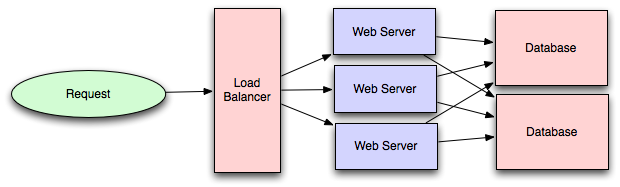
- List different services required. * Data Storage layer * eg. Usually a scalable system includes webserver (load balancer), service (service partition), database (master/slave database cluster) and caching systems.
3) Component Design
- Component + specific APIs required for each of them.
- Object oriented design for functionalities.
- Map features to modules: One scenario for one module.
- Consider the relationships among modules:
- Certain functions must have unique instance (Singletons)
- Core object can be made up of many other objects (composition).
- One object is another object (inheritance)
- Database schema design.
4) Understanding Bottlenecks
- Perhaps your system needs a load balancer and many machines behind it to handle the user requests. * Or maybe the data is so huge that you need to distribute your database on multiple machines. What are some of the downsides that occur from doing that?
- Is the database too slow and does it need some in-memory caching?
5) Scaling your abstract design
- Vertical scaling
- You scale by adding more power (CPU, RAM) to your existing machine.
- Horizontal scaling
- You scale by adding more machines into your pool of resources.
- Caching
- Load balancing helps you scale horizontally across an ever-increasing number of servers, but caching will enable you to make vastly better use of the resources you already have, as well as making otherwise unattainable product requirements feasible.
- Application caching requires explicit integration in the application code itself. Usually it will check if a value is in the cache; if not, retrieve the value from the database.
- Database caching tends to be “free”. When you flip your database on, you’re going to get some level of default configuration which will provide some degree of caching and performance. Those initial settings will be optimized for a generic usecase, and by tweaking them to your system’s access patterns you can generally squeeze a great deal of performance improvement.
- In-memory caches are most potent in terms of raw performance. This is because they store their entire set of data in memory and accesses to RAM are orders of magnitude faster than those to disk. eg. Memcached or Redis.
- eg. Precalculating results (e.g. the number of visits from each referring domain for the previous day),
- eg. Pre-generating expensive indexes (e.g. suggested stories based on a user’s click history)
- eg. Storing copies of frequently accessed data in a faster backend (e.g. Memcache instead of PostgreSQL.
- Load balancing
- Public servers of a scalable web service are hidden behind a load balancer. This load balancer evenly distributes load (requests from your users) onto your group/cluster of application servers.
- Types: Smart client (hard to get it perfect), Hardware load balancers ($$$ but reliable), Software load balancers (hybrid - works for most systems)
- Database replication
- Database replication is the frequent electronic copying data from a database in one computer or server to a database in another so that all users share the same level of information. The result is a distributed database in which users can access data relevant to their tasks without interfering with the work of others. The implementation of database replication for the purpose of eliminating data ambiguity or inconsistency among users is known as normalization.
- Database partitioning
- Partitioning of relational data usually refers to decomposing your tables either row-wise (horizontally) or column-wise (vertically).
- Map-Reduce
- For sufficiently small systems you can often get away with adhoc queries on a SQL database, but that approach may not scale up trivially once the quantity of data stored or write-load requires sharding your database, and will usually require dedicated slaves for the purpose of performing these queries (at which point, maybe you’d rather use a system designed for analyzing large quantities of data, rather than fighting your database).
- Adding a map-reduce layer makes it possible to perform data and/or processing intensive operations in a reasonable amount of time. You might use it for calculating suggested users in a social graph, or for generating analytics reports. eg. Hadoop, and maybe Hive or HBase.
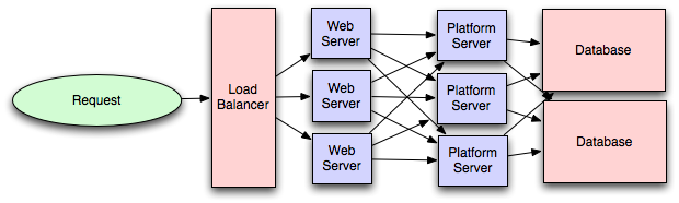
- Platform Layer (Services)
- Separating the platform and web application allow you to scale the pieces independently. If you add a new API, you can add platform servers without adding unnecessary capacity for your web application tier.
- Adding a platform layer can be a way to reuse your infrastructure for multiple products or interfaces (a web application, an API, an iPhone app, etc) without writing too much redundant boilerplate code for dealing with caches, databases, etc.
Key topics for designing a system
1) Concurrency
- Do you understand threads, deadlock, and starvation? Do you know how to parallelize algorithms? Do you understand consistency and coherence?
2) Networking
- Do you roughly understand IPC and TCP/IP? Do you know the difference between throughput and latency, and when each is the relevant factor?
3) Abstraction
- You should understand the systems you’re building upon. Do you know roughly how an OS, file system, and database work? Do you know about the various levels of caching in a modern OS?
4) Real-World Performance
- You should be familiar with the speed of everything your computer can do, including the relative performance of RAM, disk, SSD and your network.
5) Estimation
- Estimation, especially in the form of a back-of-the-envelope calculation, is important because it helps you narrow down the list of possible solutions to only the ones that are feasible. Then you have only a few prototypes or micro-benchmarks to write.
6) Availability & Reliability
- Are you thinking about how things can fail, especially in a distributed environment? Do know how to design a system to cope with network failures? Do you understand durability?
Web App System design considerations:
- Security (CORS)
- Using CDN
- A content delivery network (CDN) is a system of distributed servers (network) that deliver webpages and other Web content to a user based on the geographic locations of the user, the origin of the webpage and a content delivery server.
- This service is effective in speeding the delivery of content of websites with high traffic and websites that have global reach. The closer the CDN server is to the user geographically, the faster the content will be delivered to the user.
- CDNs also provide protection from large surges in traffic.
- Full Text Search
- Using Sphinx/Lucene/Solr - which achieve fast search responses because, instead of searching the text directly, it searches an index instead.
- Offline support/Progressive enhancement
- Service Workers
- Web Workers
- Server Side rendering
- Asynchronous loading of assets (Lazy load items)
- Minimizing network requests (Http2 + bundling/sprites etc)
- Developer productivity/Tooling
- Accessibility
- Internationalization
- Responsive design
- Browser compatibility
Working Components of Front-end Architecture
- Code
- HTML5/WAI-ARIA
- CSS/Sass Code standards and organization
- Object-Oriented approach (how do objects break down and get put together)
- JS frameworks/organization/performance optimization techniques
- Asset Delivery - Front-end Ops
- Documentation
- Onboarding Docs
- Styleguide/Pattern Library
- Architecture Diagrams (code flow, tool chain)
- Testing
- Performance Testing
- Visual Regression
- Unit Testing
- End-to-End Testing
- Process
- Git Workflow
- Dependency Management (npm, Bundler, Bower)
- Build Systems (Grunt/Gulp)
- Deploy Process
- Continuous Integration (Travis CI, Jenkins)
Links
Introduction to Architecting Systems for Scale
Scalable System Design Patterns
Scalable Web Architecture and Distributed Systems
What is the best way to design a web site to be highly scalable?
Embeddings
- Let’s start by talking about one of the most fundamental aspects of any model, it’s embedding.
- Embedding is just a lower dimensionality representation of the data. This makes it possible to perform efficient computations while minimizing the effect of the curse of dimensionality, providing more robust representations when it comes to overfitting.
- In practice, this is just a vector living in a “latent” or “semantic” space.
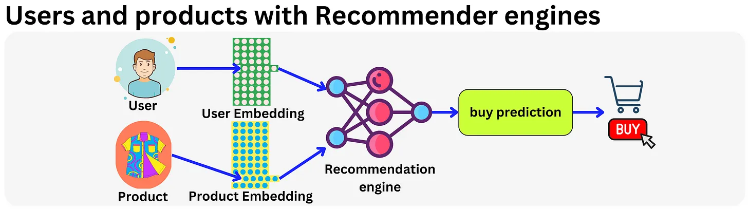
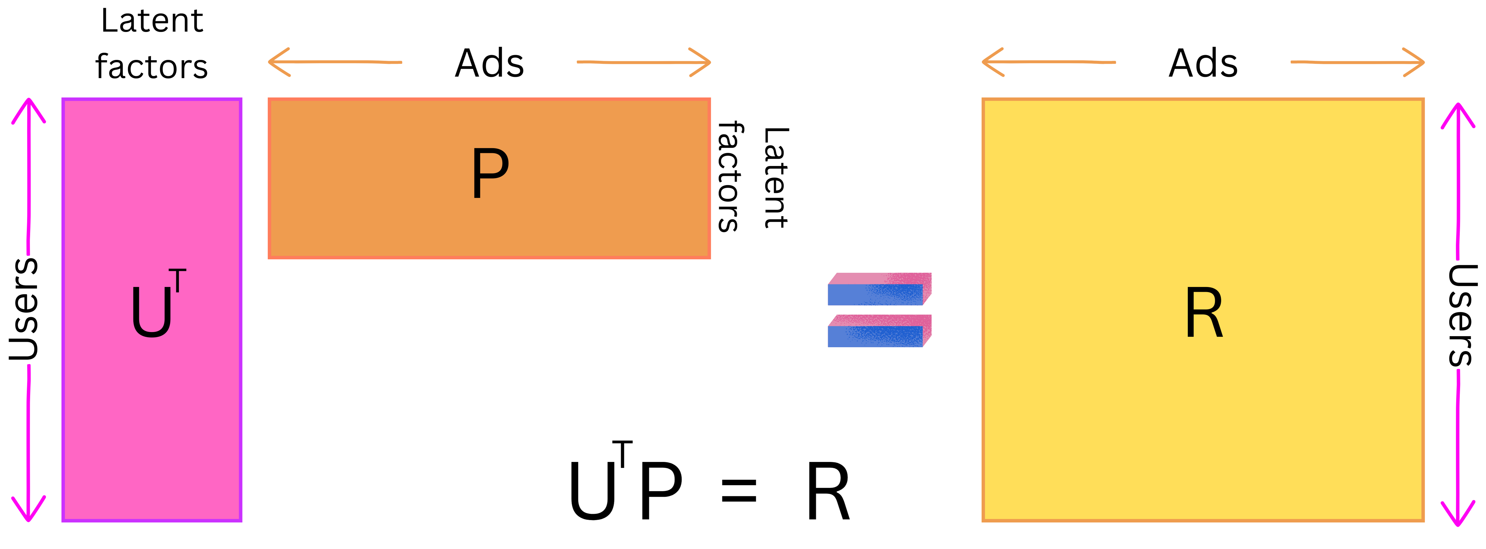
- One domain where embeddings changed everything is recommender engines. It all started with Latent Matrix Factorization methods made popular during the Netflix movie recommendation competition in 2009.
- The idea is to have a vector representation for each user and product and use that as base features. In fact, any sparse feature could be encoded within an embedding vector and modern recommender engines typically use hundreds of embedding matrices for different categorical variables.
Hashing trick
- One typical problem with embeddings is that they can consume quite a bit of memory as the whole matrix tends to be loaded at once.
- In RecSys interviews, a common question is designing a model that would recommend ads to users. A novice answer would be to draw a simple recommender engine with a user embedding and an ads embedding, a couple of non-linear interactions and a “click-or-not” learning task. But the interviewer asked “but wait, we have billions of users, how is this model going to fit on a server?!”. A naive embedding encoding strategy will assign a vector to each of the categories seen during training, and an “unknown” vector for all the categories seen during serving but not at training time. That can be a relatively safe strategy for NLP problems if you have a large enough training set as the set of possible words or tokens can be quite static.
- However, in the case of recommender systems where you can potentially have hundreds of thousands of new users every day, squeezing all those new daily users into the “unknown” category would lead to poor experience for new customers. This is precisely the cold start problem!
- A typical way to handle this problem is to use the hashing trick (“Feature Hashing for Large Scale Multitask Learning“): you simply assign multiple users (or categories of your sparse variable) to the same latent representation, solving both the cold start problem and the memory cost constraint. The assignment is done by a hashing function, and by having a hash-size hyperparameter, you can control the dimension of the embedding matrix and the resulting degree of hashing collision.
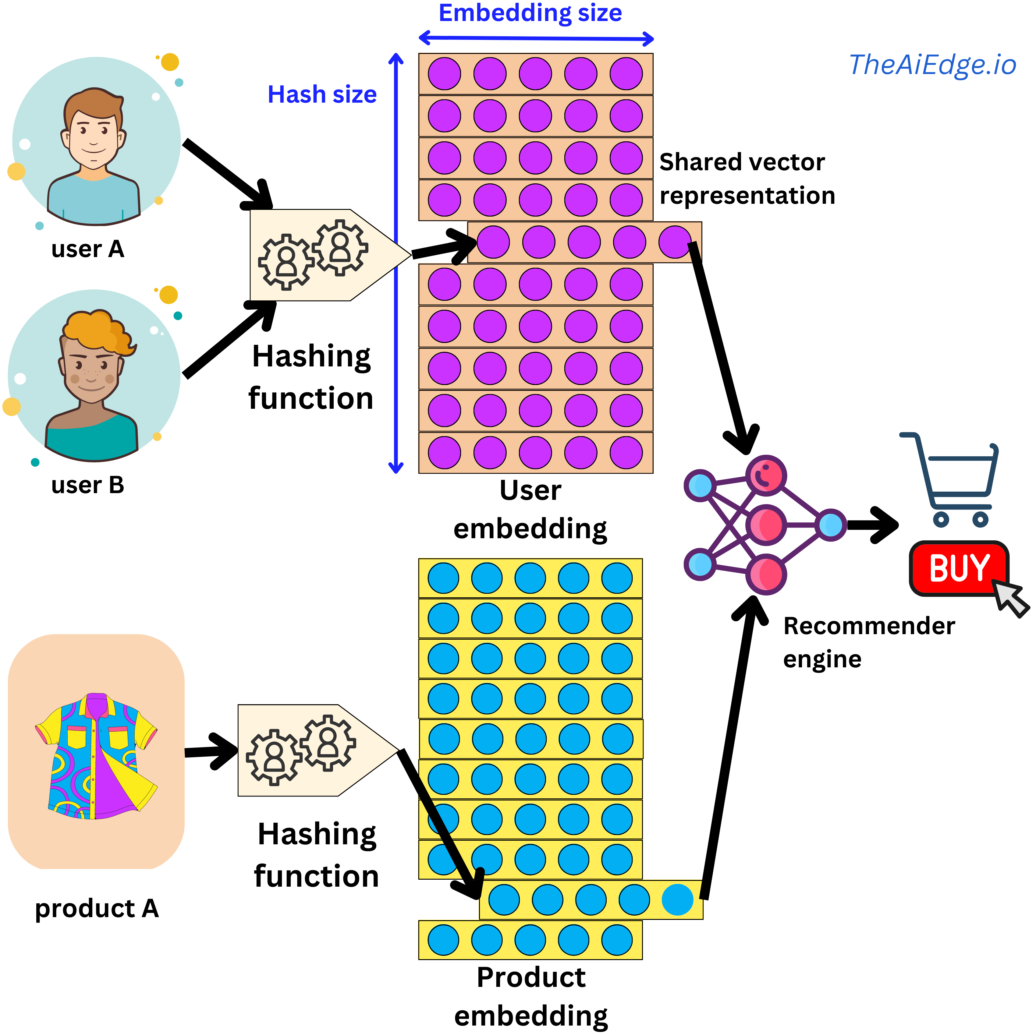
- But wait, are we not going to decrease predictive performance by conflating different user behaviors? In practice the effect is marginal. Keep in mind that a typical recommender engine will be able to ingest hundreds of sparse and dense variables, so the hashing collision happening in one variable will be different from another one, and the content-based information will allow for high levels of personalization. But there are ways to improve on this trick. For example, at Meta they suggested a method to learn hashing functions to group users with similar behaviors (“Learning to Collide: Recommendation System Model Compression with Learned Hash Functions“). They also proposed a way to use multiple embedding matrices to efficiently map users to unique vector representations (“Compositional Embeddings Using Complementary Partitions for Memory-Efficient Recommendation Systems“). This last one is somewhat reminiscent of the way a pair (token, index) is uniquely encoded in a Transformer by using the position embedding trick.
- The hashing trick is heavily used in typical recommender system settings but not widely known outside that community!
Facebook Ads Ranking
- The below content is from Damien Benveniste’s LinkedIn post.
- At Meta, we were using many paradigms of Recommendation Engines for ADS RANKING.
- Conceptually, a recommender system is simple: you take a set of features for a user \(U\) and a set of features for an item \(I\) along with features \(C\) capturing the context at the time of the recommendation (time of the day, weekend / week day, …), and you match those features to an affinity event (e.g. did the user click on the ad or not): click or not = \(F(U, I, C)\).
- In the early days they started with Gradient Boosting models. Those models are good with dense features (e.g. age, gender, number of clicks in the last month, …) but very bad with sparse features (page Id, user Id, Ad Id, …). By the way, we often talk of the superiority of Tree based models for tabular data, well this is a real exception to the rule! Those sparse features are categorical features with literally billions of categories and very few sample events. For example, consider the time series of sequence of pages visited by a user, how do you build features to capture that information? That is why they moved to Deep Learning little by little where a page Id becomes a vector in an embedding and a sequence of page Ids can be encoded by transformers as a simple vector. And even with little information on that page, the embedding can provide a good guess by using similar user interactions to other pages.
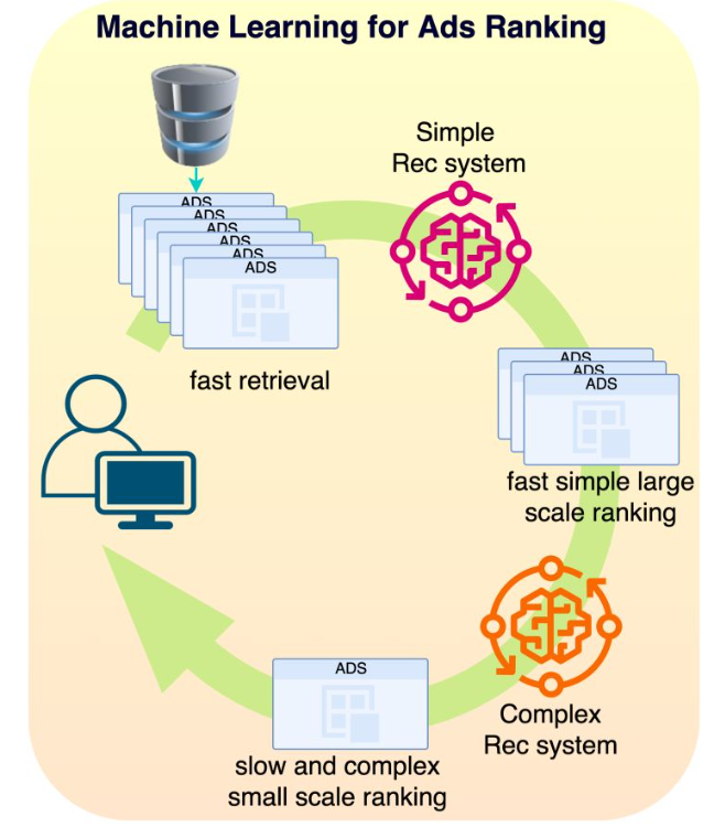
- Typical models we were using were Multi-task learning, Mixture of Experts or Multi-towers models. In Ads Ranking, the ranking happens in stages: first you select a sub-universe of ads (let’s say 1M ads) that relate to the user (very fast retrieval), then you select a subset of those ads (let’s say 1000 Ads) with a simple model (fast inference) and then you use a very complex model (slow inference) to rank the resulting ads as accurately as possible. The top ranked ad will be the one you see on your screen. We also used MIMO (multi-inputs multi-outputs) models to simultaneously train the simple and complex models for efficient two staged ranking.
- Today Facebook has about ~3 billion users and ~2 billion daily active users. It is the second largest ads provider in the world after Google. 95% of Meta’s revenue comes from ads and Facebook generates ~$70B every year while Instagram ~$50B in ads alone. There are ~15 million active advertising accounts, with approximately more than 15 million active ad campaigns running at any point in time.
- Facebook feeds contain a lists of posts interlaced with ads in between. Let’s Why is that specific ad shown to me?
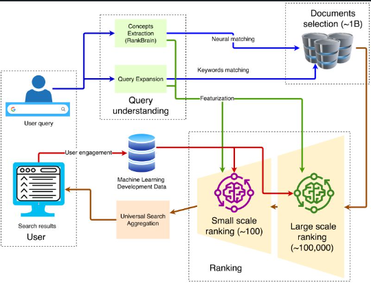
Design overview
- Conceptually, choosing the right ad for the right user is pretty simple. We pull ads from a database, rank them according to how likely the user is to click on them, run an auction process to pick the best one, and we finally present it to the user.
- The process to present one ad on the user’s screen has the following components to it:
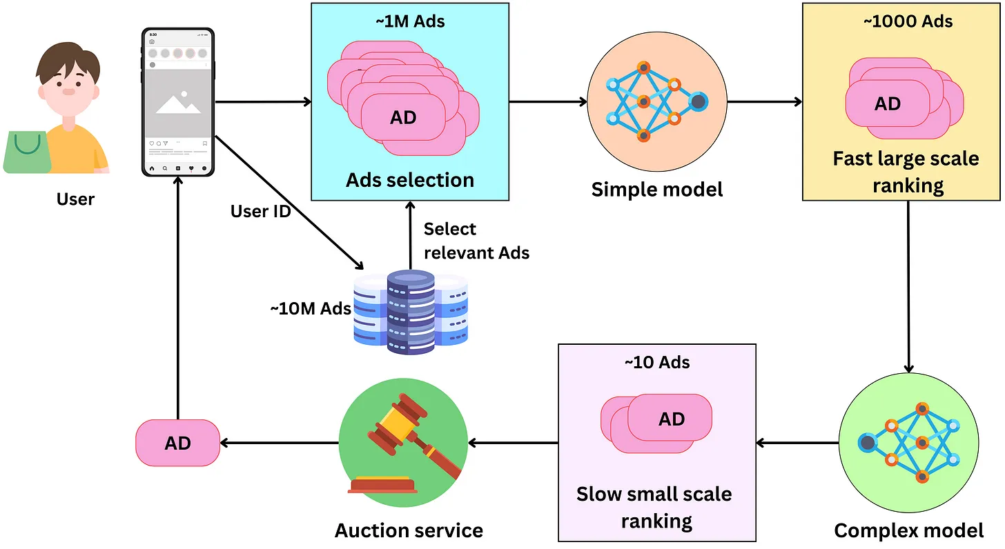
- Selecting ads: The ads are indexed in a database and a subset of them is retrieved for a specific user. At all times, there are between 10M and 100M ads and we need to filter away ads that are not relevant to the user. Meta has access to age, gender, location, or user’s interest data that can be used as keywords filters for fast ads retrieval. Additional context information can be used to further filter the selected ads. For example, if it is winter and the user lives in Canada, we could exclude ads for swim suits! We can expect this process to pull between 100K and 1M ads
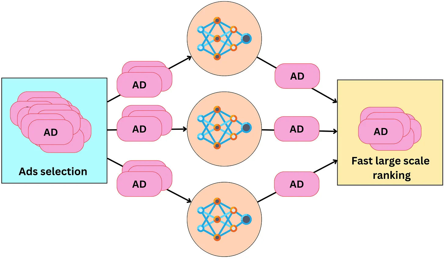
- Fast large scale ranking: With that many ads, we need to rank them in stages. Typically there are two stages: a first fast (per ad) large scale ranking stage and a slow (per ad) small scale ranking one. The first stage needs to be able to handle a large amount of ads (from the ads selection step) while being relatively fast for a low latency process. The model has usually a low capacity and uses a subset of the features making it fast. The ads are scored with a probability of being clicked by the user and only the top ads are retained for the next step. Typically this process generates between 100 and 1000 ads.
- Slow small scale ranking: This step needs to handle a smaller amount of ads, so we can use a more complex model that is slower per ad. This model, being more complex, has better predictive performance than the one in the previous step, leading to a more optimal ranking of the resulting ads. We keep only the best ranking ads for the next step. At this point, we may have of the order of ~10 remaining ads.
- The auction: An advertiser only pays Facebook when the user clicks on the ad. During the campaign creation, the advertiser sets a daily budget for a certain period. From this, we can estimate the cost he is willing to pay per click (bid) and the remaining ads are ranked according to their bid and probability of click. The winning ad is presented to the user.
Architecture
- The models used in multi-stage ranking are recommender engines. They take as inputs a set of features about the user, the ads and the context, and they output the probability that the user will click on the ads.
- The base architecture used at Facebook is the SparseNN architecture. The main components are as follows:
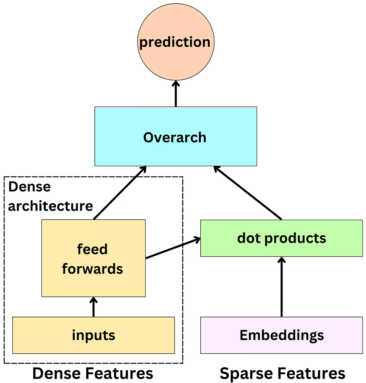
- The dense features: those are typically the continuous variables and low dimensionality categorical variables: age, gender, number of likes in the past week, …
- The sparse features: those are the high dimensionality categorical variables and they are represented by an embedding: user id, page id, ad id, …
- The dense architecture: dense features are fed to the dense architecture. Latent representations of dense features are derived from non-linear functions in dense architecture. The latent representations have the same size as sparse features’ embeddings.
- The dot product layer: reminiscent of the latent matrix factorization model, multiple dot products of pairs of dense and sparse embeddings are computed.
- The overarch: the resulting outputs are fed to a set of non-linear functions before producing a probability prediction.
Detailed architecture
- For recommender systems, there are several architecture paradigms used.
- Let’s see a few detailed below:
Multi-task learning architecture (“An Overview of Multi-Task Learning in Deep Neural Networks”)
- In the context of a recommender system, Multi-task learning (MTL) architecture can be used to improve the performance of the system by simultaneously learning to recommend multiple types of items to users.
- For example, consider a movie streaming platform that wants to recommend both movies and TV shows to its users. Traditionally, the platform would train separate recommender systems for movies and TV shows, but with MTL architecture, the platform can train a single neural network to recommend both movies and TV shows at the same time.
- In this case, the shared layers of the neural network would learn the shared features and characteristics of movies and TV shows, such as genre, actors, and directors. The task-specific layers for movies would learn the specific features and characteristics of movies that are important for making accurate recommendations, such as user ratings and movie length. Similarly, the task-specific layers for TV shows would learn the specific features and characteristics of TV shows that are important for making accurate recommendations, such as episode duration and the number of seasons.
- The neural network would be trained using loss functions specific to each task, such as mean squared error for predicting user ratings for movies, and cross-entropy loss for predicting the probability of a user watching a specific TV show.
- By using MTL architecture, the recommender system can leverage the shared structure and features across multiple types of items to improve the accuracy of recommendations for both movies and TV shows, while reducing the amount of data required to train each task.
                      Input
                        |
                  Shared Layers
                        |
               /        |         \
  Movie-specific  TV-show specific  User-specific
     Layers          Layers          Layers
       |                |               |
  Movie Loss        TV-show Loss     User Loss
       |                |               |
    Movie Output    TV-show Output   User Output
- In this architecture, the input to the neural network is user and item data, such as user ratings and item features. The shared layers of the neural network learn shared representations of the data, such as latent features that are common to both movies and TV shows.
- The movie-specific and TV-show specific layers are task-specific and learn features that are specific to movies and TV shows, respectively. For example, the movie-specific layers might learn to predict movie genres or directors, while the TV-show specific layers might learn to predict the number of seasons or the release date of a TV show.
- The user-specific layers learn features that are specific to each user, such as user preferences or viewing history. These layers take into account the user-specific data to personalize the recommendations for each user.
- Each task has its own loss function that measures the error between the predicted output and the actual output of the neural network for that task. Like we discussed earlier, the movie loss function might be mean squared error for predicting user ratings for movies, while the TV-show loss function might be cross-entropy loss for predicting the probability of a user watching a specific TV show.
- The outputs of the neural network are the predicted ratings or probabilities for each item, which are used to make recommendations to the user.
Mixture of experts (“Recommending What Video to Watch Next: A Multitask Ranking System”)
- Mixture of experts (MoE) is a type of neural network architecture that can be used for recommender systems to combine the predictions of multiple models or “experts” to make more accurate recommendations.
- In the context of a recommender system, MoE can be used to combine the predictions of multiple recommendation models that specialize in different types of recommendations. For example, one model might specialize in recommending popular items, while another model might specialize in recommending niche items.
- The MoE architecture consists of multiple “experts” and a “gate” network that learns to select which expert to use for a given input. Each expert is responsible for making recommendations for a subset of items or users. The gate network takes the input data and predicts which expert is best suited to make recommendations for that input.
- Here is an illustration of the MoE architecture for a recommender system:
                            Input
                              |
                       /     |     \
                 Expert1  Expert2  Expert3
                   |        |         |
                 Output1  Output2  Output3
                   \       |        /
                    \      |       /
                     \     |      /
                       Gate Network
                              |
                           Output
- In this architecture, the input is user and item data, such as user ratings and item features. The MoE consists of three experts, each of which is responsible for making recommendations for a subset of items or users.
- Each expert has its own output, which is a prediction of the user’s preference for the items in its subset. The gate network takes the input data and predicts which expert is best suited to make recommendations for that input. The gate network output is a weighted combination of the outputs of the three experts, where the weights are determined by the gate network.
-
The MoE architecture allows the recommender system to leverage the strengths of multiple models to make more accurate recommendations. For example, one expert might be good at recommending popular items, while another expert might be good at recommending niche items. The gate network learns to select the expert that is best suited for a given input, based on the user’s preferences and the item’s features.
- In this architecture, the input is user and item data, such as user ratings and item features. The MoE consists of three experts, each of which is responsible for making recommendations for a subset of items or users.
- Expert1 specializes in recommending popular movies, while Expert2 specializes in recommending niche TV shows, and Expert3 specializes in recommending new releases of both movies and TV shows. Each expert has its own output, which is a prediction of the user’s preference for the items in its subset.
- The gate network takes the input data and predicts which expert is best suited to make recommendations for that input. The gate network output is a weighted combination of the outputs of the three experts, where the weights are determined by the gate network.
- For example, if the input data indicates that the user has a history of watching popular movies and TV shows, the gate network might assign a higher weight to Expert1 and Expert2, and a lower weight to Expert3. The output of the MoE architecture is a ranked list of recommended items, which can include both movies and TV shows.
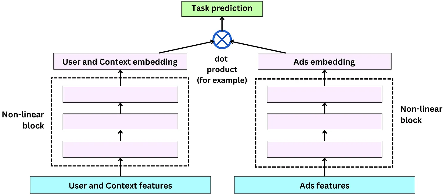
Multi-tower models (“Cross-Batch Negative Sampling for Training Two-Tower Recommenders”)
- Multi-tower models are a type of neural network architecture used in recommender systems to model the interactions between users and items. The name “multi-tower” refers to the fact that the architecture consists of multiple towers or columns, each of which represents a different aspect of the user-item interaction.
- In a two-tower architecture, there are two towers or columns: one tower represents the user and the other tower represents the item. Each tower consists of multiple layers of neurons, which can be fully connected or sparse.
- The user tower takes as input the user’s features, such as demographic information, browsing history, or social network connections, and processes them through the layers to produce a user embedding, which is a low-dimensional vector representation of the user.
- The item tower takes as input the item’s features, such as its genre, cast, or director, and processes them through the layers to produce an item embedding, which is a low-dimensional vector representation of the item.
- The user and item embeddings are then combined using a similarity function, such as dot product or cosine similarity, to produce a score that represents the predicted rating or likelihood of interaction between the user and the item.
- Here’s an example of a two-tower architecture for a movie recommender system:
                           Input
                             |
                       /          \
                 User Tower    Movie Tower
                 /   \           /     \
            Layer   Layer     Layer   Layer
              |       |         |       |
         User Age  User Gender  Genre   Director
              |       |         |       |
            Layer   Layer     Layer   Layer
              |       |         |       |
        User Embedding  Movie Embedding
                    \        /
                     \      /
                      Score
- In this architecture, the user tower and the movie tower are each represented by two layers of neurons. The user tower takes as input the user’s age and gender, which are processed through the layers to produce a user embedding. The movie tower takes as input the movie’s genre and director, which are processed through the layers to produce a movie embedding.
- The user and movie embeddings are then combined using a similarity function, such as dot product or cosine similarity, to produce a score that represents the predicted rating or likelihood of the user watching the movie.
- For example, if a user is a 30-year-old female, and the movie is a drama directed by Christopher Nolan, the user tower will produce a user embedding that represents the user’s age and gender, and the movie tower will produce a movie embedding that represents the movie’s genre and director. The user and movie embeddings are then combined using a similarity function to produce a score that represents the predicted rating or likelihood of the user watching the movie.
- The architecture can be extended to include more features, such as the user’s viewing history, the movie’s release date, or the user’s mood, to model more complex interactions between users and movies.
- As an example, the Two-tower paradigm is an extension of the more classical latent matrix factorization model. The latent matrix factorization model is a linear model where the users are represented by a matrix U and the ads by a matrix P such that the dot product R is as close as possible to the target to predict:
- Two-tower architecture allows dense and sparse features, and users (and context) and ads have their own non-linear towers. The tower output is used in a dot product to generate predictions:
Training data
Features
- When it comes to features, we need to think about the different actors of process: users, the ads and the context. Meta has ~10,000 features capturing those actors’ behavior. Let’s look at a few examples:
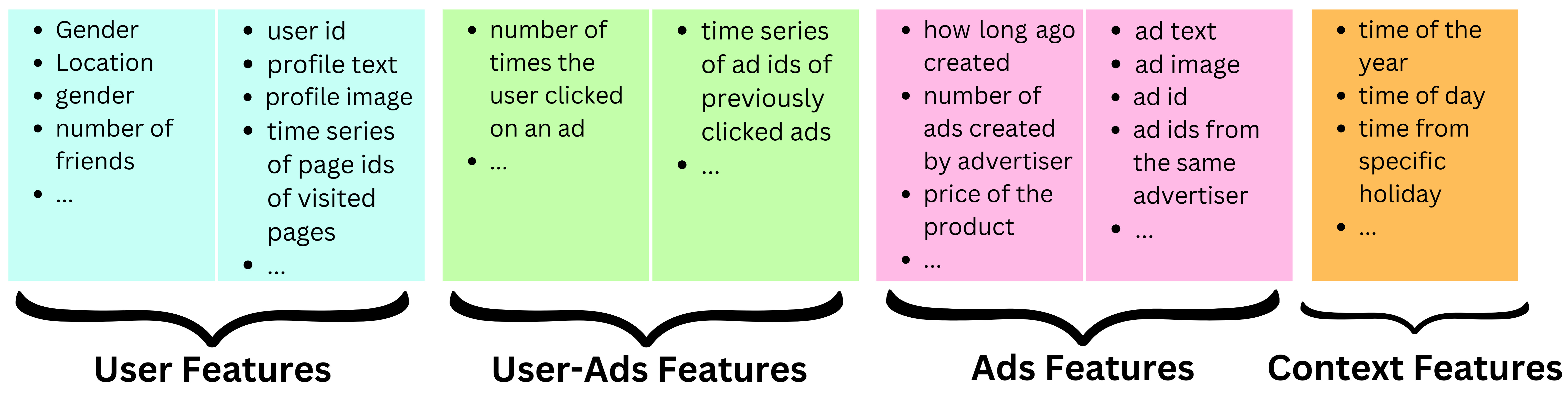
- User features: Dense features: age, gender, number of friends, number of friends with a specific interest, number of likes for pages related to a specific interest, etc.
- Embedding features: latent representation of the profile text, latent representation of the profile picture, etc.
- Sparse features: user id, time series of page ids of visited pages, user ids of closest friends, etc.
- Ads features
- Dense features: how long ago created, number of ads created by advertiser, price of the product, etc.
- Embedding features: latent representation of the ad text, latent representation of the ad image, etc.
- Sparse features: Ad id, ad ids from the same advertiser, etc.
- Context features
- Dense features: time of the year, time of day, time from specific holiday, election time of not, etc.
- User-ads interaction features
- Dense features: number of times the user clicked on an ad, number of times the user clicked on ads related to a specific subject, etc.
- Sparse features: time series of ad ids of previously clicked ads, time series of ad ids of previously seen ads, etc.
Training samples
- The problem is a binary classification problem: will the user click or not? On Facebook, there are between 1B and 2B daily active users and each user sees on average 50 ads per day. That is ~3T ads shown per month. The typical click-through rate for ads is between 0.5% and 1%. If the ad click event represent a positive sample and an ad shown but not clicked, a negative sample, that is a very imbalanced data set. Considering the size of the data, we can safely sample down the negative samples to reduce the computational pressure during training and the imbalance of the target classes.
- In a recommender system, one common approach for training a model to make predictions is to use a binary classification framework, where the goal is to predict whether a user will interact with an item or not (e.g., click on an ad or purchase a product). However, in practice, the number of negative examples (i.e., examples where the user did not interact with an item) can be much larger than the number of positive examples (i.e., examples where the user did interact with an item). This can lead to an imbalance in the data distribution, which can affect the model’s performance.
- To address this issue, one common technique is to downsample the negative examples to balance the class distribution. However, this downsampling can lead to biased probability estimates, as the probabilities of the positive examples will be overestimated, while the probabilities of the negative examples will be underestimated.
- To correct for this bias, a technique called probability calibration can be used. In this technique, the estimated probabilities are recalibrated to ensure that they are well calibrated with the true probability of the positive examples. One simple way to do this is to use a recalibration formula:
-
\[p' = p / (p + (1 - p) * s)\]
- where p is the estimated probability, s is the negative sampling rate (i.e., the ratio of negative examples to positive examples in the training data), and p’ is the recalibrated probability.
- Intuitively, this formula rescales the estimated probability p by adjusting it based on the negative sampling rate s, such that the resulting probability p’ is better calibrated with the true probability of the positive examples. This recalibrated probability can then be used in the auction process to determine which item to recommend to the user.
Metrics
Offline metrics
- Because the model is a binary classifier, it is usually trained with the cross-entropy loss function, and it is easy to use that metric to assess models.
- At Facebook, they actually use normalized entropy (“Normalized Cross-Entropy“) by normalizing the cross-entropy with the average cross-entropy.
- It is useful to assess across models and teams as anything above 1 is worse than random predictions.
- In the context of recommender systems, offline metrics refer to evaluation metrics that are computed using historical data, without actually interacting with users in real-time. These metrics are typically used during the model development and validation stage to measure the model’s performance and to compare different models.
Online metrics
- Once an engineer validates that the challenger model is better than the current one in production when it comes to the offline metrics, we can start the A/B testing process to validate the model on production data. The Ads Score metric used in production is a combination of the total revenue generated by the model and a quality metric measured by how often the users hide or report an ad.
- Online metrics refer to evaluation metrics that are computed in real-time using actual user interactions with the recommender system.
Low correlation of online and offline metrics
- The goal of using both offline and online metrics is to ensure that the models that perform well on offline metrics also perform well in production, where they interact with real users. However, in practice, there is often a low correlation between the performance of models on offline and online metrics.
- For example, a model that performs well on an offline metric, such as normalized entropy, may not perform well on an online metric, such as Ads Score, which measures how well the model performs in terms of user engagement and conversion. This could be due to various reasons, such as the difference between the data distribution in the offline and online environments, the presence of feedback loops in the online environment, and the lack of personalization in the offline experiments.
- To address this issue, active research is ongoing to create offline metrics that have a higher correlation with the online metrics. One approach is to incorporate user feedback and engagement data into the offline experiments to better simulate the online environment. Another approach is to use more advanced machine learning models, such as deep learning architectures, that can better capture the complex relationships between user behavior and item recommendations. Ultimately, the goal is to develop offline metrics that can better predict the performance of models in the online environment, and to improve the overall effectiveness of recommender systems.
The auction
The winning ad
- The auction process is used to reorder the top predicted ads taking into account the bid put on those ads by the advertisers and the quality of those ads.
- The bid is the maximum amount an advertiser is willing to pay for a single click of their ad.
- p(user will click) is the calibrated probability coming out of the recommender engine.
- Ad quality is an estimate of the quality of an ad coming out of another machine learning model. This model is trained on the events when users reported or hid an ad instead of click events.
- The advertiser is charged only when a user clicks on the ad, but the cost does not exactly correspond to the bid. The advertiser is charged the minimum price needed to win the auction with a markup of $0.01. This is called cost per click (CPC).
Bid computed
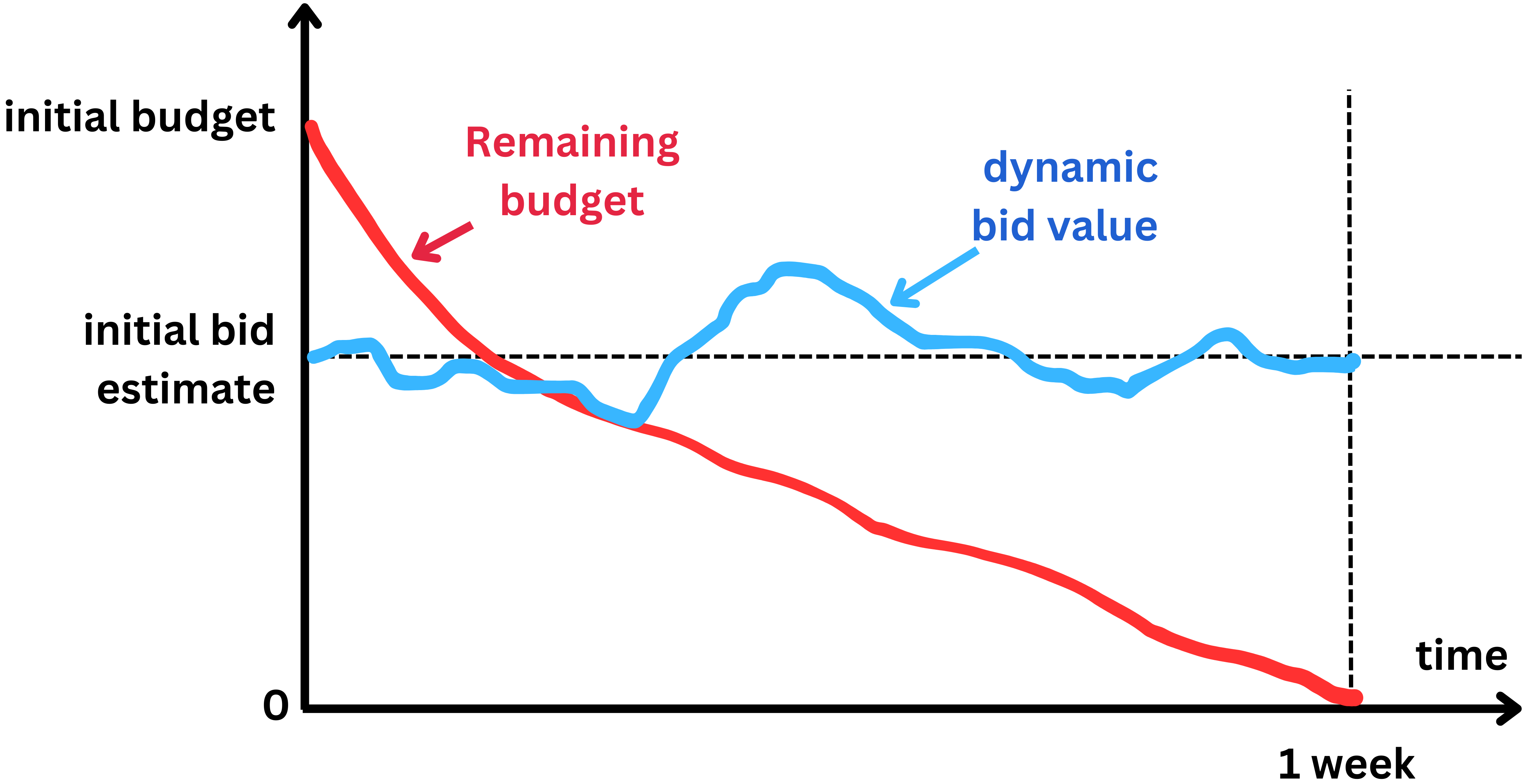
- When it comes to an ad campaign, the advertiser does not provide a bid value but a budget in dollar amount for certain period of time.
- For example $100 for one week. Because Facebook knows how many other campaigns are happening at the time, they can estimate how many times they are likely to show the ad, let’s say 5000 times per day, or 35,000 times in 7 days.
- If the click-through rate is 1%, the number of ad clicks will be 35,000 x 0.01 = 350. And $100 / 350 = $0.3. So based on budget and average click through rate statistics, Facebook can estimate an initial bid value.
- To ensure the ad click-through rate is in line with the set budget and the timeline, the bid value can be dynamically adjusted such that the budget is not exhausted too fast or too slowly. If the budget is consumed faster than expected the bid will be decreased by a small factor, and if the remaining budget is still too high, the bid can be artificially increased.
The Serving pipeline
Scaling
- The ranking process can easily be distributed to scale with the number of ads. The different models can be duplicated and the ads distributed among the different replicas. This reduce the latency of the overall process.
Pre-computing
- The ranking process does not need to be realtime. Being able to pre-compute the ads is cheaper since we don’t need to use as many machines to reduce the latency and we can use bigger models (so slower) which will improve the ranking quality. The reason we may want to be close to a real-time process is to capture the latest changes in the state of the user, ads or context.
- In reality, the features associated with those actors will change marginally in a few minutes The cost associated to be real-time may not be worth the gain, especially for users that rarely click on ads. There are several strategies we can adopt to reduce operating costs:
- In the context of advertising, the ranking process refers to the process of selecting and ordering the ads that will be displayed to a user based on their interests, preferences, and other relevant factors. This ranking process can be performed either in real-time, where the ads are selected and ordered on-the-fly as the user interacts with the platform, or in a pre-computed manner, where the ads are selected and ordered ahead of time and stored for future use.
- The statement “The ranking process does not need to be realtime” suggests that pre-computing the ads can be a more cost-effective approach than performing the ranking process in real-time. This is because pre-computing the ads allows for the use of bigger and more complex models that can improve the quality of the ad ranking, while reducing the number of machines needed to process the requests, thus reducing the cost.
- However, being close to a real-time process can be important in order to capture the latest changes in user behavior, ads, and context, and to ensure that the ads being displayed are relevant and engaging. This is particularly important for users who frequently click on ads and are more likely to engage with the platform.
- To balance the trade-off between the cost and the effectiveness of the ad ranking process, several strategies can be adopted. For example, one approach is to use a hybrid approach that combines pre-computed ads with real-time updates based on user behavior and contextual information. Another approach is to focus on improving the accuracy of the ad ranking models and algorithms, which can help to reduce the number of ads that need to be displayed to achieve the desired level of engagement. Finally, optimizing the infrastructure and resource allocation can also help to reduce the cost of performing the ad ranking process in real-time.
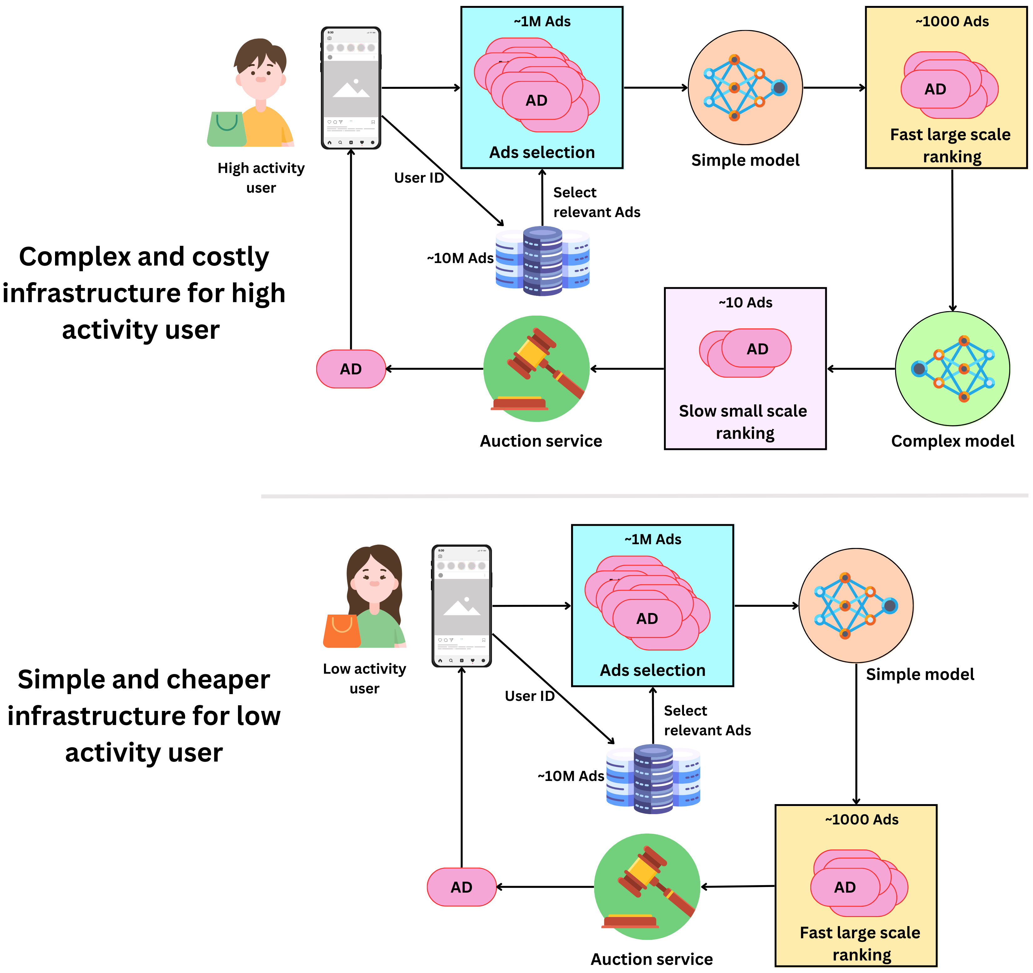
- Users can be tiered:
- some users, no matter what, will never click on an ad, while others will do so very often. For low activity users, we could set up a low cost / low accuracy infrastructure to minimize the cost per ranking for users that don’t generate much revenue. For high-activity users, the cost of accurate predictions is worth the gain.
- We can use more powerful models and low- latency infrastructures to increase their likelihood to click on ads.
- Users can be tiered:
- We don’t know much about new users:
- it might be unnecessary to try to generate accurate rankings for users we don’t know much about as the models will be likely to be wrong. Initially, newly created users could be classified as low activity users until we have enough data about them to generate accurate rankings.
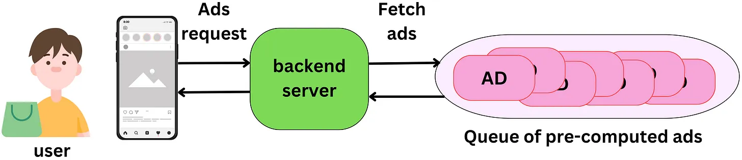
- Pre-computing ads for a user session:
- User sessions typically require multiple ads to be shown. It feels like a waste of resources to rank millions of ads every time an ad is shown. One ranking process can produce an array of ready-to-go ads for each user session.
- Finding the right triggers:
- If we want to pre-compute ads rankings a few minutes or hours in advance, we need to find the right triggers to do so.
- We could recompute the ads ranking in a scheduled manner, for example each hour we run the ranking for the 3B Facebook users. That seems like a waste of resources if the user doesn’t log in for a week let’s say!
- We could start the process at the moment the user logs in. This way the ads are ready by the time the user scrolls to the first ad position. This works if the ranking process is fast enough.
- We could recompute the ranking every time there is a significant change in the user’s state. For example the user liked a page related to a specific interest or registered for a new group. If the user is not very active, we could combine this strategy with the scheduled one by recalculating the ranking after a certain period.
Twitter’s Recommendation Algorithm
- The foundation of Twitter’s recommendations is a set of core models and features that extract latent information from Tweet, user, and engagement data. These models aim to answer important questions about the Twitter network, such as, “What is the probability you will interact with another user in the future?” or, “What are the communities on Twitter and what are trending Tweets within them?” Answering these questions accurately enables Twitter to deliver more relevant recommendations.
- The recommendation pipeline is made up of three main stages that consume these features:
- Fetch the best Tweets from different recommendation sources in a process called candidate sourcing.
- Rank each Tweet using a machine learning model.
- Apply heuristics and filters, such as filtering out Tweets from users you’ve blocked, NSFW content, and Tweets you’ve already seen.
- The service that is responsible for constructing and serving the For You timeline is called Home Mixer. Home Mixer is built on Product Mixer, our custom Scala framework that facilitates building feeds of content. This service acts as the software backbone that connects different candidate sources, scoring functions, heuristics, and filters.
- This diagram below illustrates the major components used to construct a timeline:
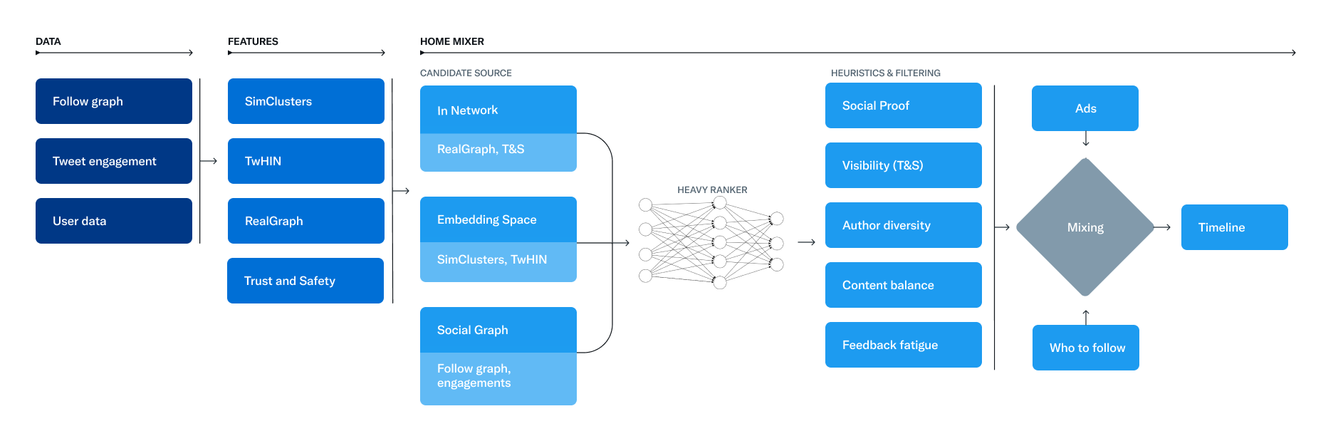
- Let’s explore the key parts of this system, roughly in the order they’d be called during a single timeline request, starting with retrieving candidates from Candidate Sources.
Candidate Sources
- Twitter has several Candidate Sources that we use to retrieve recent and relevant Tweets for a user. For each request, we attempt to extract the best 1500 Tweets from a pool of hundreds of millions through these sources. We find candidates from people you follow (In-Network) and from people you don’t follow (Out-of-Network).
- Today, the For You timeline consists of 50% In-Network Tweets and 50% Out-of-Network Tweets on average, though this may vary from user to user.
In-Network Source
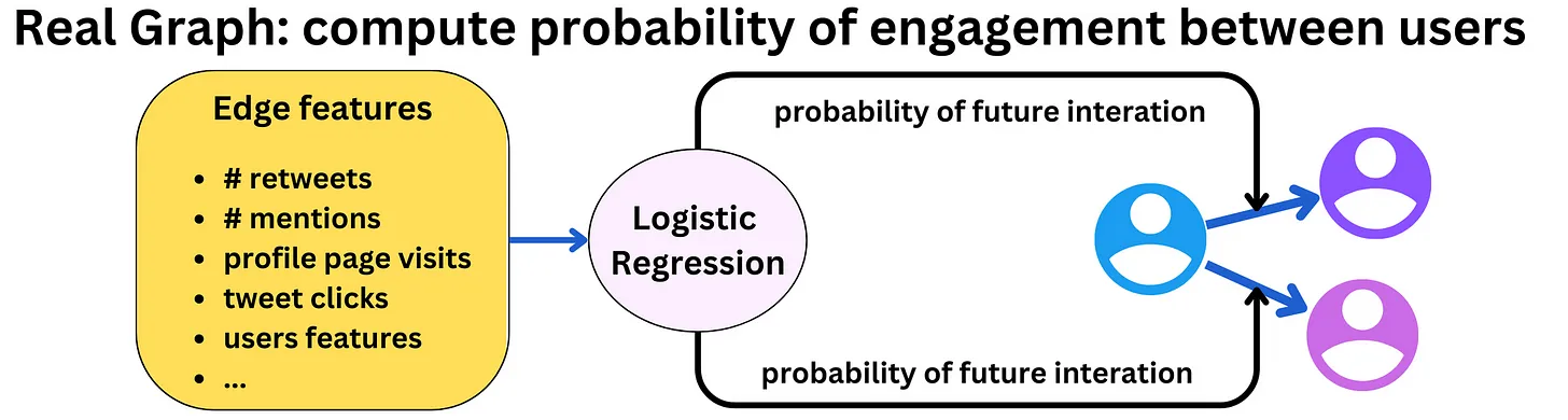
- The In-Network source is the largest candidate source and aims to deliver the most relevant, recent Tweets from users you follow. It efficiently ranks Tweets of those you follow based on their relevance using a logistic regression model. The top Tweets are then sent to the next stage.
- The most important component in ranking In-Network Tweets is Real Graph. Real Graph is a model which predicts the likelihood of engagement between two users. The higher the Real Graph score between you and the author of the Tweet, the more of their tweets we’ll include.
- The In-Network source has been the subject of recent work at Twitter. We recently stopped using Fanout Service, a 12-year old service that was previously used to provide In-Network Tweets from a cache of Tweets for each user. We’re also in the process of redesigning the logistic regression ranking model which was last updated and trained several years ago!
Out-of-Network Sources
- Finding relevant Tweets outside of a user’s network is a trickier problem: How can we tell if a certain Tweet will be relevant to you if you don’t follow the author? Twitter takes two approaches to addressing this.
Social Graph
- Our first approach is to estimate what you would find relevant by analyzing the engagements of people you follow or those with similar interests.
- We traverse the graph of engagements and follows to answer the following questions:
- What Tweets did the people I follow recently engage with?
- Who likes similar Tweets to me, and what else have they recently liked?
- We generate candidate Tweets based on the answers to these questions and rank the resulting Tweets using a logistic regression model. Graph traversals of this type are essential to our Out-of-Network recommendations; we developed GraphJet, a graph processing engine that maintains a real-time interaction graph between users and Tweets, to execute these traversals. While such heuristics for searching the Twitter engagement and follow network have proven useful (these currently serve about 15% of Home Timeline Tweets), embedding space approaches have become the larger source of Out-of-Network Tweets.
Embedding Spaces
- Embedding space approaches aim to answer a more general question about content similarity: What Tweets and Users are similar to my interests?
- Embeddings work by generating numerical representations of users’ interests and Tweets’ content. We can then calculate the similarity between any two users, Tweets or user-Tweet pairs in this embedding space. Provided we generate accurate embeddings, we can use this similarity as a stand-in for relevance.
- One of Twitter’s most useful embedding spaces is SimClusters. SimClusters discover communities anchored by a cluster of influential users using a custom matrix factorization algorithm. There are 145k communities, which are updated every three weeks. Users and Tweets are represented in the space of communities, and can belong to multiple communities. Communities range in size from a few thousand users for individual friend groups, to hundreds of millions of users for news or pop culture. These are some of the biggest communities:
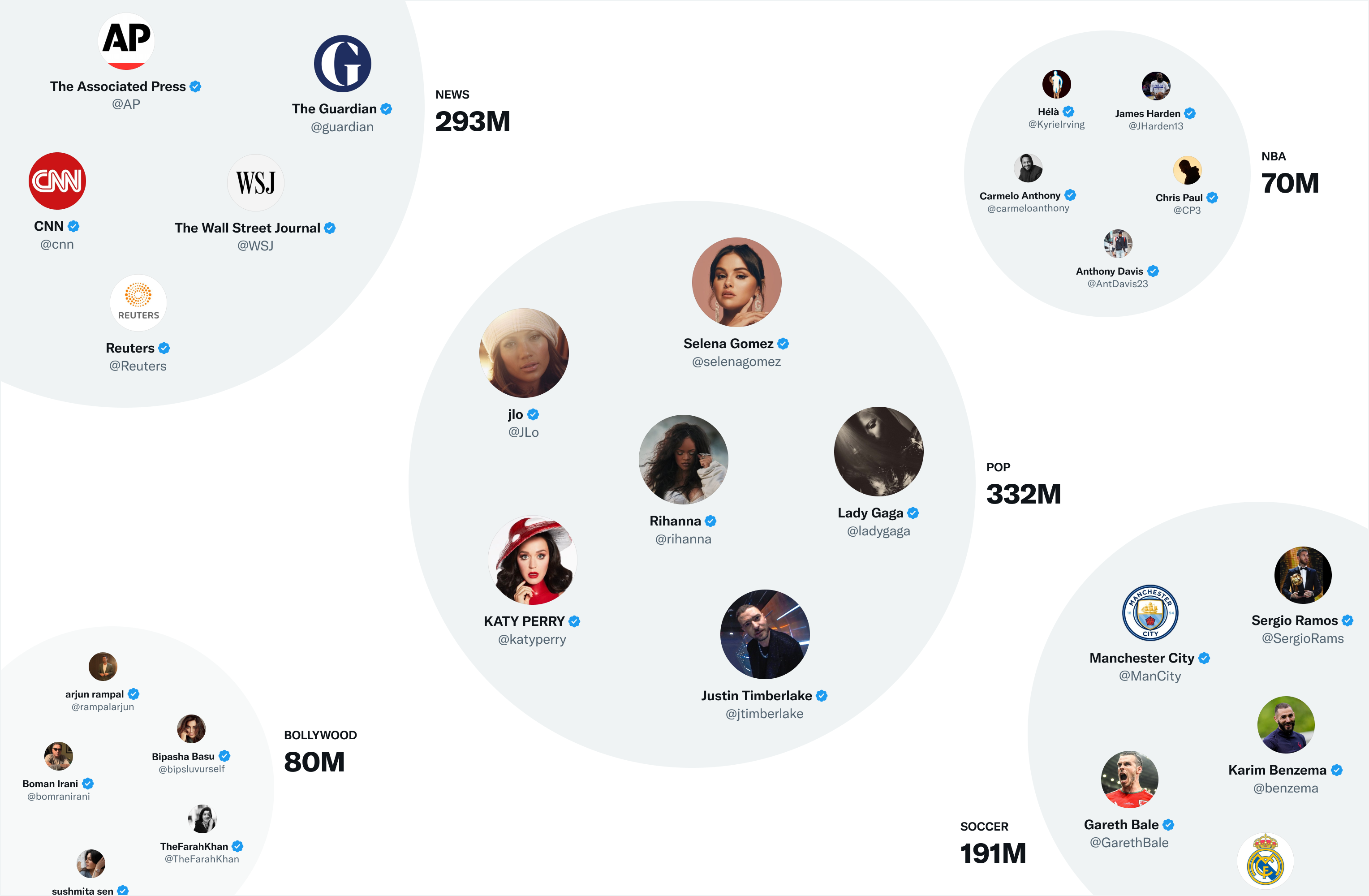
- We can embed Tweets into these communities by looking at the current popularity of a Tweet in each community. The more that users from a community like a Tweet, the more that Tweet will be associated with that community.
Ranking
- The goal of the For You timeline is to serve you relevant Tweets. At this point in the pipeline, we have ~1500 candidates that may be relevant. Scoring directly predicts the relevance of each candidate Tweet and is the primary signal for ranking Tweets on your timeline. At this stage, all candidates are treated equally, without regard for what candidate source it originated from.
- Ranking is achieved with a ~48M parameter neural network that is continuously trained on Tweet interactions to optimize for positive engagement (e.g. Likes, Retweets, and Replies). This ranking mechanism takes into account thousands of features and outputs ten labels to give each Tweet a score, where each label represents the probability of an engagement. We rank the Tweets from these scores.
Heuristics, Filters, and Product Features
- After the Ranking stage, we apply heuristics and filters to implement various product features. These features work together to create a balanced and diverse feed. Some examples include:
- Visibility Filtering: Filter out Tweets based on their content and your preferences. For instance, remove Tweets from accounts you block or mute.
- Author Diversity: Avoid too many consecutive Tweets from a single author.
- Content Balance: Ensure we are delivering a fair balance of In-Network and Out-of-Network Tweets.
- Feedback-based Fatigue: Lower the score of certain Tweets if the viewer has provided negative feedback around it.
- Social Proof: Exclude Out-of-Network Tweets without a second degree connection to the Tweet as a quality safeguard. In other words, ensure someone you follow engaged with the Tweet or follows the Tweet’s author.
- Conversations: Provide more context to a Reply by threading it together with the original Tweet.
- Edited Tweets: Determine if the Tweets currently on a device are stale, and send instructions to replace them with the edited versions.
Mixing and Serving
- At this point, Home Mixer has a set of Tweets ready to send to your device. As the last step in the process, the system blends together Tweets with other non-Tweet content like Ads, Follow Recommendations, and Onboarding prompts, which are returned to your device to display.
- The pipeline above runs approximately 5 billion times per day and completes in under 1.5 seconds on average. A single pipeline execution requires 220 seconds of CPU time, nearly 150x the latency you perceive on the app.
- The goal of our open source endeavor is to provide full transparency to you, our users, about how our systems work. We’ve released the code powering our recommendations that you can view here (and here) to understand our algorithm in greater detail, and we are also working on several features to provide you greater transparency within our app. Some of the new developments we have planned include:
- A better Twitter analytics platform for creators with more information on reach and engagement
- Greater transparency into any safety labels applied to your Tweets or accounts
- Greater visibility into why Tweets appear on your timeline
Twitter’s Retrieval Algorithm: Deep Retrieval
- The content here is from Damien Benveniste’s LinkedIn post.
- At a high level, Twitter’s recsys works the same as most, it takes the “best” tweets, ranks them with an ML model, filters the unwanted tweets and presents it to a user.
- Let’s delve deeper into Twitter’s ML algorithm that go through multistage tweet selection processes for ranking.
- Twitter first selects about 1500 relevant tweets with 50% coming from your network and 50% from outside.
- For the 50% in your network, they then use Real Graph to rank people within your network which internally is a logistic regression algorithm running on Hadoop.
- The features used here are previous retweets, tweet interactions and user features and with these, they compute the probability that the user will interact with these users again.
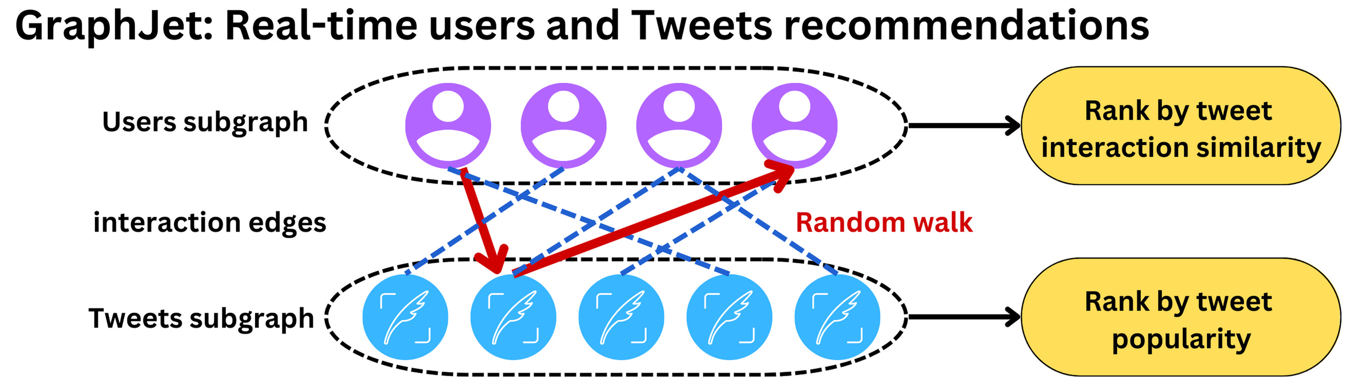
- For the 50% out of network, they use GraphJet.
- “Different users and tweet interactions are captured over a certain time window and a SALSA algorithm (random walk on a bipartite graph) is run to understand the tweets that are likely to interest some users and how similar users are to each other. This process leads to metrics we can rank to select the top tweets.” (source)
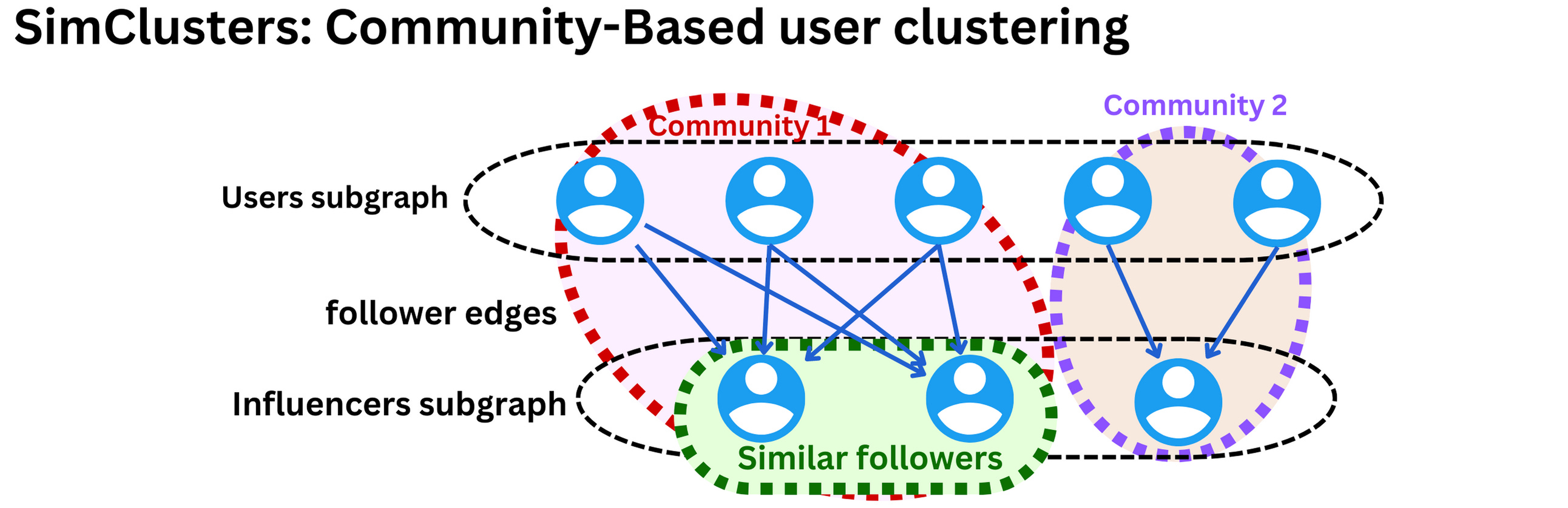
- SimClusters algorithm: “clusters users into communities. The idea is to assign similarity metrics between users based on what influencers they follow. With those clusters, we can assign users’ tweets to communities and measure similarity metrics between users and tweets.” (source)
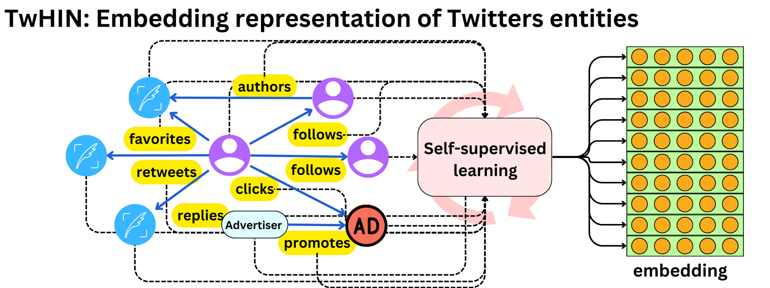
- TwHIN algorithm:is a more modern graph algorithm to compute latent representations (embeddings) of the different Twitter entities (users, tweets, ads, advertisers) and the relationships between those entities (clicks, follows, retweets, authors, etc.). The idea is to use contrastive learning to minimize the dot products of entities that interact in the graph and maximize the dot-product of entities that do not. (source)
- Once the recommendations are selected, they are ranked via a 48M parameters MaxNet model that includes thousands of features and 10 engagement labels to compute a final score to rank tweets.
- The image below (source) illustrates these different methodologies at play.
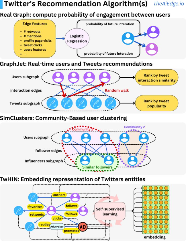
- Twitter just open-sourced its recommendation algorithm for personalized tweet feeds and it is pretty much what you would expect: you get the “best” tweets, rank them with a machine learning model, filter the unwanted tweets and present them to the user.
- That is the way that most recommender engines tend to be used: search engines, ads ranking, product recommendation, movie recommendation, etc. What is interesting is the way the different Twitter’s ML algorithms come together to be used as multistage tweet selection processes for the ranking process.
- The first step in the process is to select ~1500 relevant tweets, 50% coming from people in your network and 50% outside of it. Real Graph (“RealGraph: User Interaction Prediction at Twitter“) is used to rank people in your network. It is a logistic regression algorithm running on Hadoop. Using features like previous retweets, tweet interactions and user features we can compute the probability that a specific user will interact again with other users.
- For people outside your network, they use GraphJet, a real-time graph recommender system.
- Different users and tweet interactions are captured over a certain time window and a SALSA algorithm (random walk on a bipartite graph) is run to understand the tweets that are likely to interest some users and how similar users are to each other.
- SALSA is similar to a personalized PageRank algorithm but adapted to multiple types of objects recommendation. This process leads to metrics we can rank to select the top tweets.
- The SimClusters algorithm (“SimClusters: Community-Based Representations for Heterogeneous Recommendations at Twitter“) clusters users into communities.
- The idea is to assign similarity metrics between users based on what influencers they follow. With those clusters, we can assign users’ tweets to communities and measure similarity metrics between users and tweets.
- The TwHIN algorithm (“TwHIN: Embedding the Twitter Heterogeneous Information Network for Personalized Recommendation“) is a more modern graph algorithm to compute latent representations (embeddings) of the different Twitter entities (users, tweets, ads, advertisers) and the relationships between those entities (clicks, follows, retweets, authors, …). The idea is to use contrastive learning to minimize the dot products of entities that interact in the graph and maximize the dot-product of entities that do not. [Embeddings can be used to compute user-tweet similarity metrics and be used as features in other models.]
- Once those different sources of recommendation select a rough set of tweets, we rank them using a 48M parameters MaskNet model (“MaskNet: Introducing Feature-Wise Multiplication to CTR Ranking Models by Instance-Guided Mask“).
- Thousands of features and 10 engagement labels are used to compute a final score to rank tweets.
- For more information, take a look at the Twitter blog (Twitter’s Recommendation Algorithm) and the GitHub repo.
TikTok Recommender System
- The unique problem TikTok has is that the training data is non-stationary as a user’s interest can change in a matter of minutes and the number of users, ads, videos are also constantly changing.
- “The predictive performance of a recommender system on a social media platform deteriorates in a matter of hours, so it needs to be updated as often as possible.” (source)
- The high level overview of how TikTok works is:
- A user opens the app and sends a request to the TikTok service to populate videos in their feed.
- TikTok’s service requests feed ranking from the recommender engine.
- During retrieval, the first stage will select a set of relevant video candidates for that user and select the top 100 or so videos. The candidate generation step here consists of both Deep Retrieval and a simple linear model.
- The second stage is a fine ranking of the candidates selected with the first video being the one with the highest score.
- Finally, the list is sent to the user, the image below (source) illustrates this process completely.
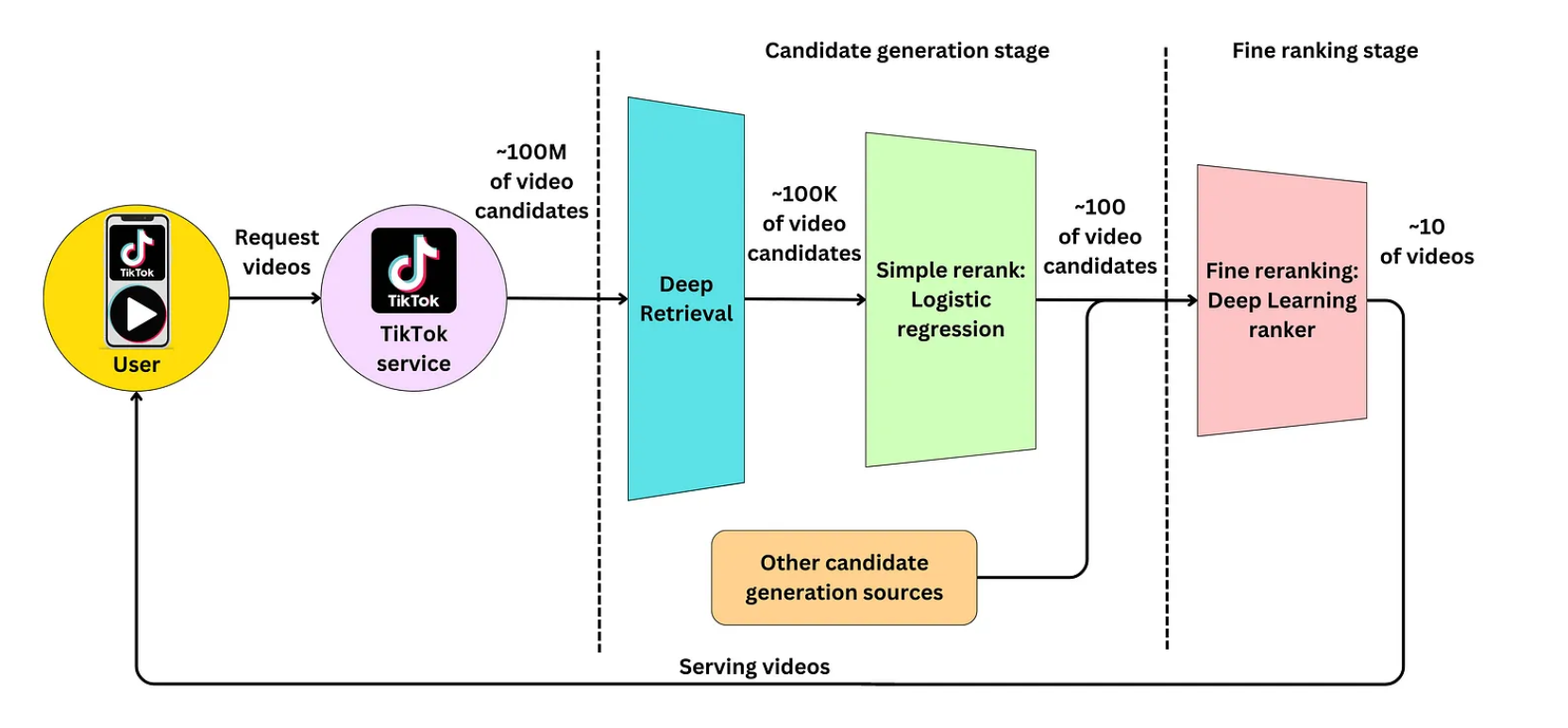
Collisionless hashing
- TikTok is continuously learning online in order to keep the recommendations fresh and the model server generates features for the model to recommend.
- It does this via a feedback loop that processes where the user interacts with the recommended items generated by the model server, and their behavior is used to update the model parameters. Specifically, the user feedback in the form of interactions with the recommended videos (e.g., likes, shares, comments) is collected and sent to the training server, where it is used to generate new training samples. These new samples are then used to update the model parameters in the parameter server, which are then synchronized with the production model every minute. This continuous feedback loop enables the recommender system to adapt to the rapidly changing user behavior on the platform, improving the accuracy of the recommendations over time.
- In a typical recommender system, sparse variables such as users, videos, and ads are assigned to fixed embedding tables using a hash function. However, this approach can be limited in terms of the model’s performance because multiple categories may get assigned to the same vector, which can lead to user behavior getting conflated. Additionally, this approach limits the memory size that can be allocated to the table.
- To address these limitations, TikTok uses dynamic embedding sizes. This means that each new user is assigned to their own vector instead of sharing a vector with multiple users. TikTok uses a collision-less hashing function to ensure that each user gets their unique vector.
-
To optimize memory usage, low-activity users are removed from the embedding table dynamically. This helps to keep the embedding table small while preserving the quality of the model. By dynamically adjusting the size of the embedding table and using unique vectors for each user, TikTok’s recommender system is better able to handle new users and optimize model performance.
- Recommender systems need to predict highly on sparse categorical variables. TikTok has ~1B active users and ~100M videos available on the platform, both represented by categorical variables. Once you build new features from those, the number of sparse variables increases. Building models using those variables can be challenging because we typically use embedding tables to encode them. This adds a lot of memory load on the serving servers.
- Recommender engines typically use the hashing trick (“Feature Hashing for Large Scale Multitask Learning“): you simply assign multiple users (or categories of your sparse variable) to the same latent representation, solving both the cold start problem and the memory cost constraint. The assignment is done by a hashing function. By having a hash-size hyperparameter, you can control the dimension of the embedding matrix and the resulting degree of hashing collision. Conflating user behaviors will reduce the predictive performance and organizations need to weight the memory cost versus the predictive performance gain.
- TikTok took the drastic approach to eliminate hashing collisions by combining two methods. First, they avoid using computational resources for users without enough data for reasonable statistical learning, and then implement their own custom collisionless hashing method.
The Cuckoo Hashmap
- They use the Cuckoo hashing method to resolve collisions. The idea is to keep in memory two large enough hash tables such that if collisions happen in the first table, the items get kicked to the second table and the process iterates until all collisions are resolved. The process converges in O(1). Let’s consider the following example:
- A new user A needs to be encoded in the embedding table. User A is hashed into the first hashmap but a collision with user B occurs.
- User B is kicked out of table 1 and hashed into the second table but a collision with user C occurs.
- User C is kicked out of table 2 and hashed into the first table but a collision occurs with user D.
- 17User D is kicked out of table 1 and hashed into the second table where he finds an empty spot.
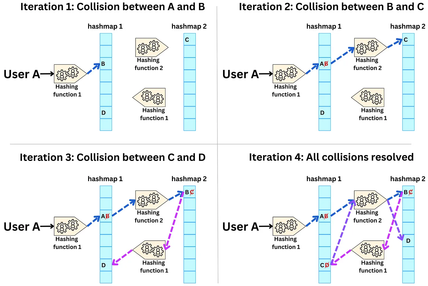
Dynamic size embeddings
- In a recommender system, the embedding tables store vector representations of users, items, or other features that the model is trained on. Typically, these embedding tables have a fixed size, which means that even if a user has not used the app for a long time or has barely interacted with it, their vector representation is still stored in memory, taking up valuable resources.
- To address this issue, TikTok uses a dynamic size embedding approach. This means that users are only accepted into the embedding tables if there are enough data points from them to statistically learn from them. The occurrence threshold is a hyperparameter that determines the minimum number of interactions required for a user to be included in the embedding table.
- Furthermore, to free up memory and keep the embeddings up-to-date, TikTok sets a predetermined period of inactivity after which a vector representation expires. This ensures that the embedding tables only store representations for active and relevant users, items, or features. Overall, dynamic size embeddings allow TikTok to efficiently manage resources and provide accurate recommendations to users.
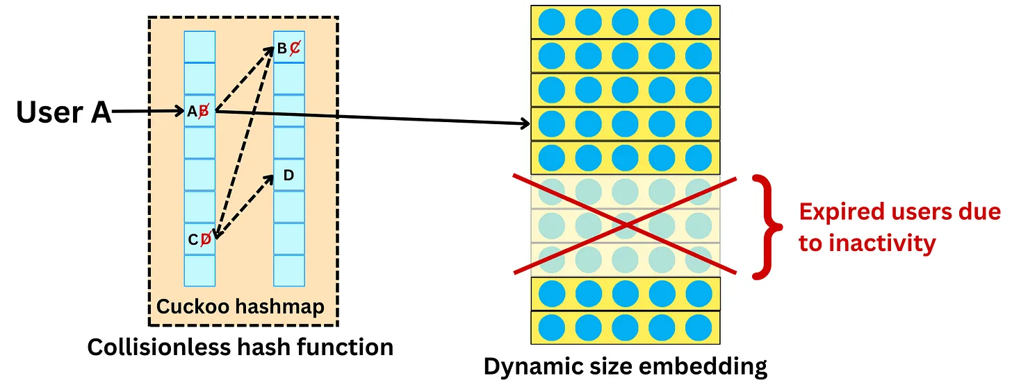
- This is an effective way to save memory costs, but it is also a balance between cost and how many users we are willing to remove from those embedding tables. It will affect the predictive performance if too many users are not modeled.
Instantaneous updates during runtime
- TikTok is very large, with a size of several terabytes. This means that it can be very slow to synchronize the entire model across the network, which can impact the efficiency and effectiveness of the model. To overcome this challenge, the model is only partially updated.
- The main reason for the partial update is because of the issue of non-stationary or concept drift. This occurs because the model relies on embedding tables to represent sparse variables such as users, videos, and ads. When a user interacts with a recommended item, only the embedding vectors associated with the user and the item are updated, along with some the weights on the network.
- Therefore, instead of synchronizing the entire model every minute, only the updated embedding vectors are synchronized on a minute-by-minute basis, while the network weights are synchronized on a longer time frame. This approach enables the system to continuously adapt to changing user behavior without the need for frequent full model synchronization, which can be time-consuming and inefficient.
Sparse variables:
- Sparse variables are variables that have a large number of possible values, but only a small subset of these values are present in the data at any given time. In the context of recommender systems, examples of sparse variables include users, items, and features of items.
- Users: There are millions of users on the platform, but any given user has only rated or interacted with a small subset of movies.
- Movies: There are thousands of movies in the database, but any given user has only rated or interacted with a small subset of them.
- Genres: There are many movie genres, but any given movie may only belong to a small subset of them.
Conflated categories:
- Conflated, in the context of recommender systems, refers to the phenomenon where multiple different values or categories of a sparse variable get assigned to the same vector. This can happen when using fixed embedding tables and a hash function to assign categories to vectors. When categories get conflated, it means that the model can’t differentiate between different categories or values, and this can result in poor performance. For example, if multiple users are assigned to the same vector, the model may not be able to distinguish between the preferences and behaviors of different users.
- Users: If the system uses a fixed embedding table and a hash function to assign users to vectors, some users may end up sharing the same vector. This means that the system can’t differentiate between the preferences and behaviors of different users who share the same vector.
- Genres: If the system uses a fixed embedding table and a hash function to assign genres to vectors, some genres may end up being assigned to the same vector. This means that the system can’t differentiate between movies that belong to different genres that share the same vector.
-
Directors: If the system uses a fixed embedding table and a hash function to assign directors to vectors, some directors may end up being assigned to the same vector. This means that the system can’t differentiate between movies that are directed by different people who share the same vector.
- The image below (source) illustrates all of these points.
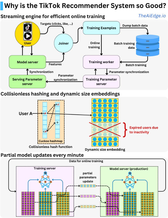
Candidate generation stage
- The candidate generation stage has to generally be fast considering the number of videos that exist, it’s usually the ranking that is slow but it deals with fewer candidates.
Deep Retrieval Model (DR)
- A typical approach to candidate generation is to find features for users that relate to features of the items.
- This is done by analyzing user behavior data and item metadata to identify relevant features and then finding relationships between them.
- For example, if we have a movie recommendation system, we can identify features of movies such as genre, actors, director, release year, and rating. We can also analyze user behavior data such as movies they have watched and rated, time of day, and day of the week they typically watch movies.
- We can then find relationships between these features by using techniques such as collaborative filtering, content-based filtering, or a combination of both. Collaborative filtering involves finding similarities between users based on their past behavior and recommending items that similar users have liked. Content-based filtering, on the other hand, involves recommending items that have similar features to items that the user has liked in the past.
- By finding features for users that relate to features of the items, we can generate a set of candidate items that are likely to be relevant to the user. This approach has been shown to be effective in many recommendation systems, as it allows us to make personalized recommendations based on the user’s preferences and behavior.
- “For example, in a case of a search engine, a user that lives in New York and that is looking for restaurant is most likely looking for those in New York. So we could potentially discard websites that relate to restaurants in other countries filtering searches beyond New York.” (source)
- “We could look at a latent representation of the user and find item latent representations that are close using approximate nearest neighbor search algorithms. These approaches require us to iterate over all the possible items which can be computationally expensive. TikTok has hundreds of millions of videos to choose from.” (source)
- Deep Retrieval instead takes in a user as the input for the model and outputs a candidate!
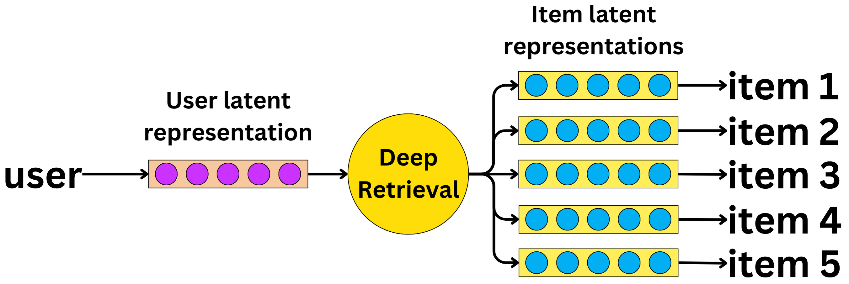
- As the image shows above, we can think of DR as a graph where beam search is used during inference for retrieval. Let’s look at the DR steps:
- A user ID is converted into its latent representation from an embedding table.
- The Deep Retrieval model learns the latent representations of related items.
- The item representations are mapped back to the items themselves, the item being an ad or video here that can be shown illustrated below.
+--------------------------------------------------------+
|                     DR Structure                        |
|                                                        |
|     Path 1                Path 2          ...    Path K |
|    +-----+               +-----+                    +-----+
|    |     |               |     |                    |     |
|    |     |               |     |                    |     |
|    |     |               |     |                    |     |
|    +-----+               +-----+                    +-----+
|    |     |               |     |                    |     |
|    |     |               |     |                    |     |
|    |     |               |     |                    |     |
|    +-----+               +-----+                    +-----+
|       :                    :                           :
|       :                    :                           :
|    +-----+               +-----+                    +-----+
|    |     |               |     |                    |     |
|    |     |               |     |                    |     |
|    |     |               |     |                    |     |
|    +-----+               +-----+                    +-----+
|                                                        |
|                      Mapping Tables                     |
|                                                        |
| Path 1: Item 1, Item 2, ..., Item M1                    |
| Path 2: Item 3, Item 4, ..., Item M2                    |
|    :                          :                          |
| Path K: Item N1, Item N2, ..., Item Nk                  |
+--------------------------------------------------------+
- Each path represents a cluster of items and a probability distribution is learned over the paths based on user inputs, along with a mapping from the items to the paths.
- During the serving stage, the DR structure uses beam search to retrieve the most probable paths and the items associated with those paths. The structure is designed for retrieval rather than ranking, meaning that items within a path are considered indistinguishable for retrieval purposes, which helps mitigate the data scarcity problem. Additionally, each item is indexed by more than one path, allowing for multiple-to-multiple encoding between items and paths, which differs from the one-to-one mapping used in earlier tree-based structures.
- In TikTok’s Deep retrieval system, a probability distribution is learned over the possible paths in the DR structure, based on the user inputs. This means that given a user’s query or request, the system will learn which paths are most likely to be relevant to that query.
- At the same time, the system also learns a mapping from the items (such as videos or user profiles) to the relevant paths in the DR structure. This mapping allows the system to efficiently retrieve the items that are most relevant to the user’s query.
- By jointly learning the probability distribution over paths and the mapping from items to paths, TikTok’s Deep retrieval system can effectively cluster and retrieve items based on user inputs. This allows for a more personalized and relevant user experience on the TikTok platform.
- The mapping between paths and items in TikTok’s Deep retrieval system is typically stored in memory, rather than a database. During training, the system learns the mapping by optimizing the neural network parameters using an expectation-maximization (EM) algorithm. These learned parameters, which include the mapping between items and paths, are then stored in memory and used during inference to efficiently retrieve items based on the retrieved paths.
- The mapping is typically stored in memory as tables or arrays, which allow for efficient lookup and retrieval of item indices based on the retrieved path indices. However, depending on the scale of the system and the number of items being indexed, it may be necessary to use a distributed system or a combination of memory and disk-based storage to handle the large volume of data.
- ou can think of the DR structure as a graph where each node represents a path and the edges represent the connections between the paths. Each path is associated with a set of items, which can be thought of as the values stored at the nodes of the graph.
- During inference, the system uses beam search to traverse the graph and retrieve the most probable paths for a given user query. The retrieved paths are then used to retrieve the associated items, which are merged into a set of candidate items for ranking.
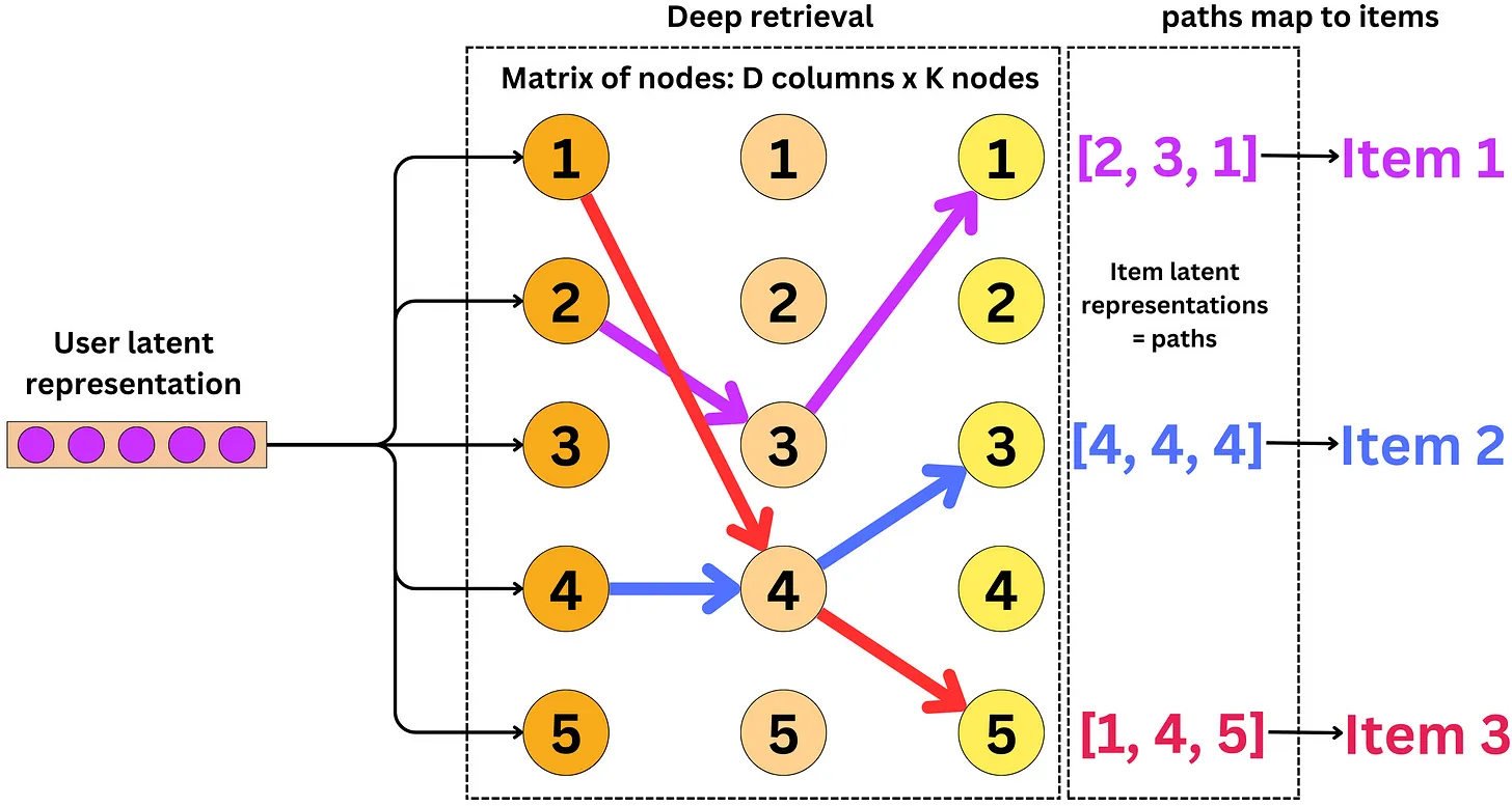
Expectation Maximization
- In the training stage, the item paths in the DR structure are learned together with the other neural network parameters of the model using an Expectation-Maximization (EM) type algorithm.
- The EM algorithm is used to optimize the parameters of the model by iteratively estimating the distribution of the latent variables (in this case, the item paths) and maximizing the likelihood of the observed data (in this case, the user-item interaction data).
- In the E-step of the algorithm, the expected value of the latent variables is computed given the current estimate of the model parameters. In the M-step, the model parameters are updated to maximize the expected log-likelihood of the data.
- This process is repeated iteratively until the convergence criterion is met. The end result is a set of optimized model parameters, including the item paths, that can be used for retrieval during the serving stage.
Matrix Abstraction to Neural Network
- Deep Retrieval’s underlying machine learning model is a neural network, which is represented as a matrix. Each column of this matrix corresponds to a specific item in the system, and the values in the matrix represent the relationship between the items based on user interactions.
- However, this matrix is just an abstraction built on top of the actual neural network model. Each column of the matrix is actually represented by a multi-layer perceptron (MLP) followed by K softmax functions, where K is the number of output nodes.
- The input to each layer of the MLP is the output of the previous layer concatenated with all the outputs from the previous layers. This allows the network to capture complex relationships between the items and to incorporate information from previous layers into the current layer.
- The output of each layer of the MLP is then passed through K softmax functions, which convert the output values into probabilities that represent the likelihood of each item being relevant to the user. The final layer outputs a K-dimensional vector for each item, and the input to this layer contains K x D values, where D is the dimensionality of the input features.
                                 User Input
                                      |
                                      v
                                  Input Layer
                                      |
                                      v
          ------------------------------------------------------
         |           |           |           |           |       |
         v           v           v           v           v       v
        Item 1      Item 2     ...        Item i    ...     Item N
         |           |           |           |           |       |
         v           v           v           v           v       v
        MLP 1       MLP 2     ...         MLP i     ...     MLP N
         |           |           |           |           |       |
         v           v           v           v           v       v
      Softmax1    Softmax2   ...        Softmaxi ...    SoftmaxN
         |           |           |           |           |       |
         v           v           v           v           v       v
        Prob1       Prob2     ...         Probi    ...     ProbN
         |           |           |           |           |       |
         v           v           v           v           v       v
         ---------------------------------------------
        |            |             |             |            |
        v            v             v             v            v
      Path 1       Path 2       Path 3       Path 4       Path K
        |            |             |             |            |
        v            v             v             v            v
      Item 1       Item 2       Item 3       Item 4       Item 5
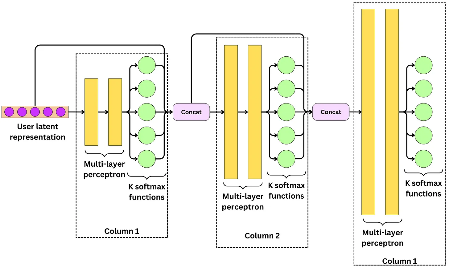
- As we see above, At the first layer, the softmax functions estimate the probability
- Then at the second layer, the softmax functions estimate the probability
- At the last layer, the softmax functions estimate the probability
- At each layer, if you followed the path of maximum probability as follows then each user would correspond to one path which in turn would lead to only one recommendation, which is a limited option!
Beam search for inference
- What we want is to input one user and get ~100K video candidates as a result.
- The strategy adopted is to use Beam search. At each layer, we follow the top B paths that maximize the probability where B is a hyperparameter. We just need to choose B ~ 100K.
Inputs: user x, beam size B

for column i in all D columns:
   C = the top B paths with highest p(c[i]|x, c[1], ..., c[i-1])

return C
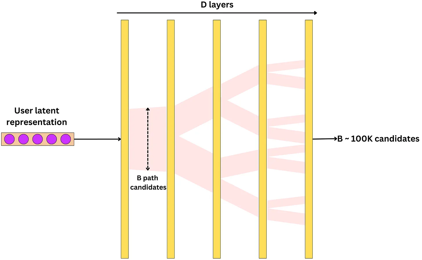
How to rank
- The probability of a path {c1, c2, …, cD} given a user is computed by applying the chain rule of probability to decompose the probability of the whole path into the product of the probabilities of each node given its predecessors and the user input.
- The model weights are learned by maximizing the log-likelihood of the problem, which means that the model tries to maximize the probability of the observed data (i.e., the paths) given the input.
- In practice, it is possible that multiple items are associated with the same path, which can cause ambiguity in the ranking. To address this issue, the authors add a penalty term to the objective function that penalizes paths with multiple items. This penalty term subtracts a factor proportional to the fourth power of the number of items associated with a path, multiplied by a coefficient α.
- However, even after adding the penalty term, it is still possible for multiple items to be associated with the same path. To address this, the authors jointly train a simple model using a softmax output function to predict which item the user will watch, given a path and the user input. This model is trained as a classifier and can be a logistic regression for low latency inference. The output of the model is a probability that can be used to rank the items retrieved from the beam search.
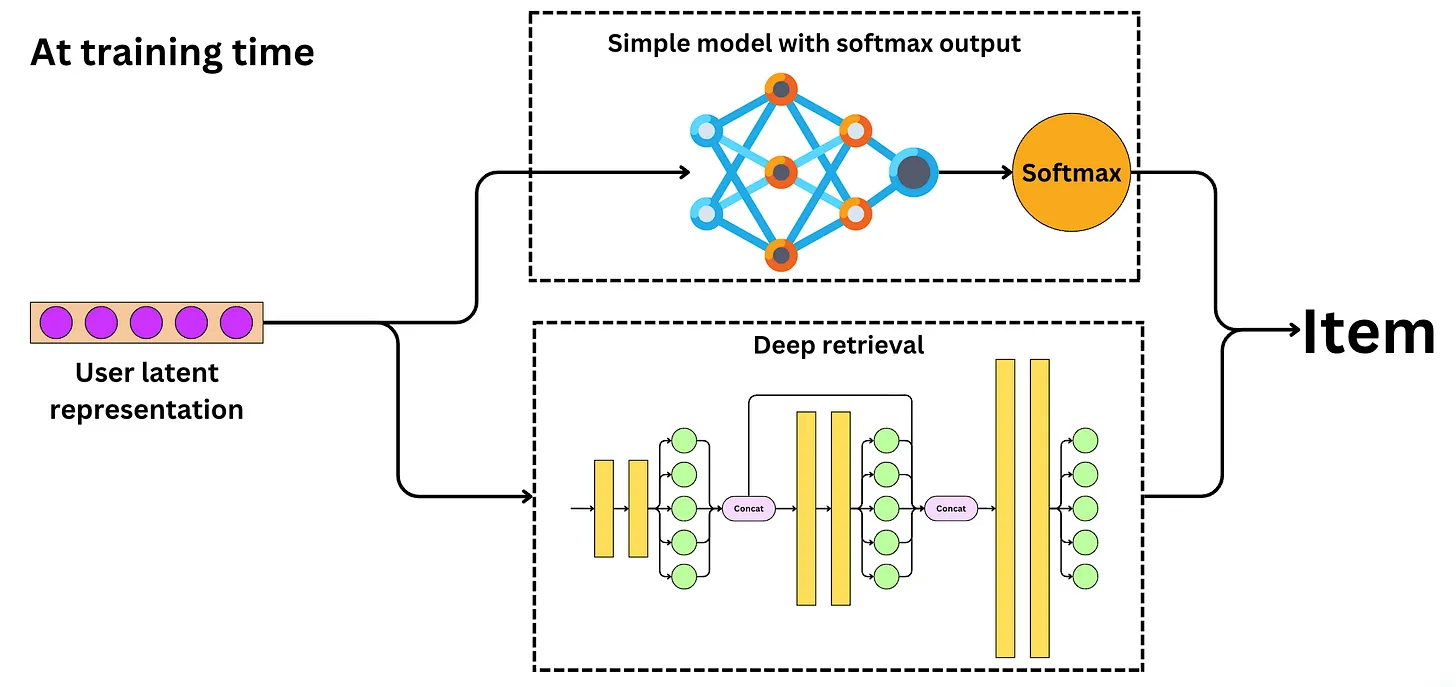
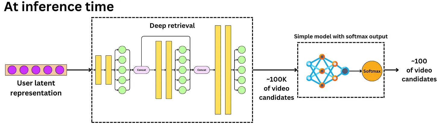
Training the model
- The Deep Retrieval model cannot be trained with gradient descent because mapping an item to a path is a discrete process. The problem is not established as a supervised learning problem because the loss function does not explicitly account for a ground truth target. We use the likelihood maximization principle to find paths that are likely to relate to a user, with those paths mapping to items. We try to learn parameters that make the model likely to represent the user-item pairs in the data.
- This is very similar to the way we approach clustering problems. Here, we try to learn paths that represent user-item pairs. The paths can be thought as clusters and the problem is solved using the Expectation-Maximization algorithm:
- Expectation: backpropagate the loss function.
- Maximization: find path mapping using only the highest probability paths in a beam search manner.
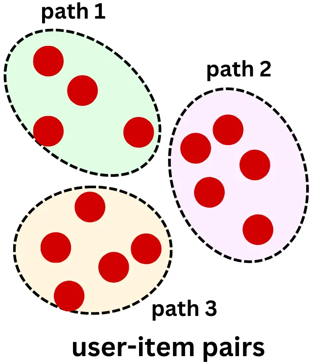
Fine ranking stage
- The candidate selection component must be optimized for latency and recall. We need to make sure all relevant videos are part of the candidate pool even if that means including irrelevant videos.
- Moreover, in most near real-time recommender systems, candidates are ranked by linear or low capacity models.
- On the other hand, we need to optimize the fine re-ranking component for precision to ensure all videos are relevant. Latency is less of a problem as we only have to rank ~100 videos. For that component, models are typically larger with higher predictive performance.
Multi-gate Mixture of Experts
- TikTok’s machine learning infrastructure is quite complex and it leverages machine learning to improve user engagement. Given the large size of TikTok’s user base, the company relies on an army of machine learning engineers to test and develop multiple machine learning models simultaneously. The ultimate goal of these models is to identify videos that will be popular with users and increase their engagement with the platform.
- TikTok uses a variety of signals to measure user engagement with videos, such as likes, comments, watch time, and subscriptions. These signals can be used as input features to machine learning models. The models score videos based on these signals simultaneously, meaning that they take into account all the positive signals to determine the video’s overall popularity. By using multiple models in parallel and considering multiple positive signals, TikTok can better predict which videos are likely to be popular with users and tailor its recommendations accordingly.
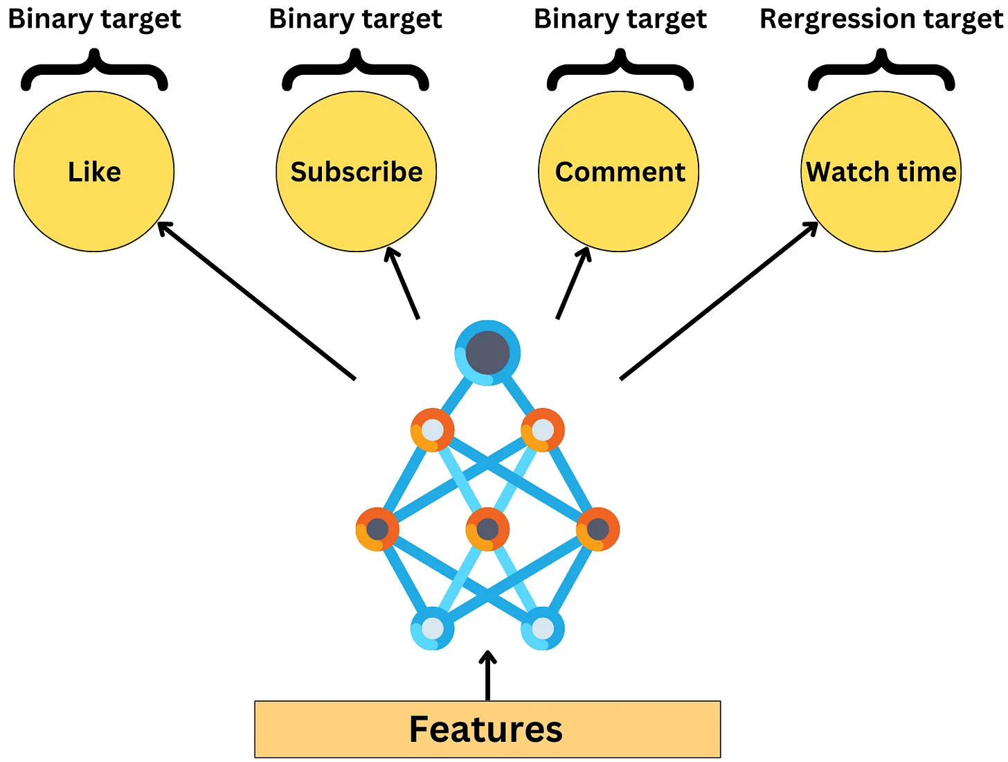
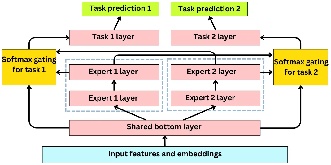
- All input features are passed through a shared layer.
- For each learning task (like, comment, subscribe, watch time), an independent tower of multiple layers is created. In principle, those layers can be anything such as multi-layer perceptrons, Transformers, … This allows the network to learn very different relationships to the targets in each tower.
- Each learning task has its own Softmax gate using all tower outputs as input. The Softmax gate is a way to weigh differently the output of each tower to learn a specific target. Each Softmax gate learns a matrix W that projects the shared bottom layer x to have the same dimensions as the number of targets:
- Let’s call the output of the ith tower fi(x). The Softmax gate output is a weighted average of the tower outputs where g(i)(x) is the ith component of g(x) and k is the number of learning tasks.
- Each Softmax feeds into a layer specific learning task, each having its own loss function.
- The specific losses are backpropagated up the Softmax gates and then summed to update the rest of the network.
- To compute a ranking score, one must combine scores for each target. Imagine, for instance, a simple linear combination of the scores
Correcting selection bias
- Selection bias in recommender systems refers to a situation where the recommendation algorithm is biased towards certain items or users, leading to a skewed distribution of recommendations. This bias can occur when the system is trained on a dataset that is not representative of the actual user population, or when the system relies on incomplete or biased user feedback data.
- For example, if a recommender system only recommends popular items or items that are frequently interacted with, then it may not be providing diverse recommendations that reflect the true preferences of the user population. Similarly, if the system relies only on explicit user feedback such as ratings or reviews, it may not be capturing the full range of user preferences and could be biased towards certain types of users.
- Selection bias is a major problem in ranking problems since users will interact with the first video and ignore the later ones thus, the videos further down the recommended list artificially receive less signal.
- This will bias the training data for future model development iterations. TikTok can be used on a mobile device as well as on an iPad or desktop computer. Each device behaves differently regarding selection bias.
- When ranking a set of recommended items, the position of each item in the list is used as a feature in the model to adjust for the bias caused by the tendency of users to prefer the items at the top of the list. By incorporating position as a feature, the model can learn to adjust the predicted probability of a user interacting with an item based on its position in the list, which can help to reduce the impact of selection bias on the model’s performance.
- To address this issue, a common approach is to train a separate model that learns the effect of position and other relevant factors, such as the user’s device or the time of day, on the user’s engagement with the recommended items. This model is trained on data that includes the position and other relevant features as input, as well as the user’s engagement with the recommended items as the output.
- The output of this model is then used to adjust the predictions of the main ranking model, effectively correcting for the bias introduced by position and other factors. This can be done by appending a shallow model parallel to the main ranking model, which takes the position and other features as input and outputs a correction factor that is applied to the main model’s predictions. By decoupling the effect of selection bias from the rest of the learning problem and giving more importance to the relevant features, this approach can lead to more accurate recommendations that are less affected by biases.
- The output of the two models, the main ranking model and the shallow model that corrects for position bias, are combined using a weighted linear combination. The weight assigned to the shallow model’s output depends on the device and position of the video in the recommended list. The final output is the combined score, which is used to rank the videos and determine the order in which they are presented to the user.
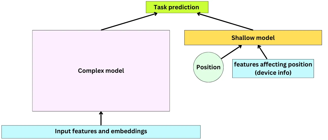
- This is an example of late fusion.
Sampling the data for Offline training
- Recommender engines typically produce very imbalanced machine learning problems. TikTok will need to show lots of videos before one clicks “like”, leaves a comment, or engages in a recommended ad. Positive engagements are usually used as positive samples in binary classification problems. Considering the amount of daily users and the amount of videos watched every day, it becomes necessary to sample down the negative samples. Negative samples are those in which the user did not provide a signal indicating their affinity for the video or advertisement.
- In a recommender system, negative samples are items that the user did not interact with or did not like. When training a model, it is important to provide both positive and negative samples to help the model learn to differentiate between them. However, not all negative samples are equally informative. TikTok uses a non-uniform negative sampling scheme that gives more weight to samples that are more likely to be positive. This means that the model is exposed to more confusing samples that are closer to the decision boundary, providing more information about the learning problem. By focusing on learning how to separate true positive samples from negative samples that look like positive ones, the model can better learn to make accurate recommendations.
- The non-uniform negative sampling scheme was developed in collaboration with the University of Connecticut and has been shown to be more effective than traditional uniform negative sampling.
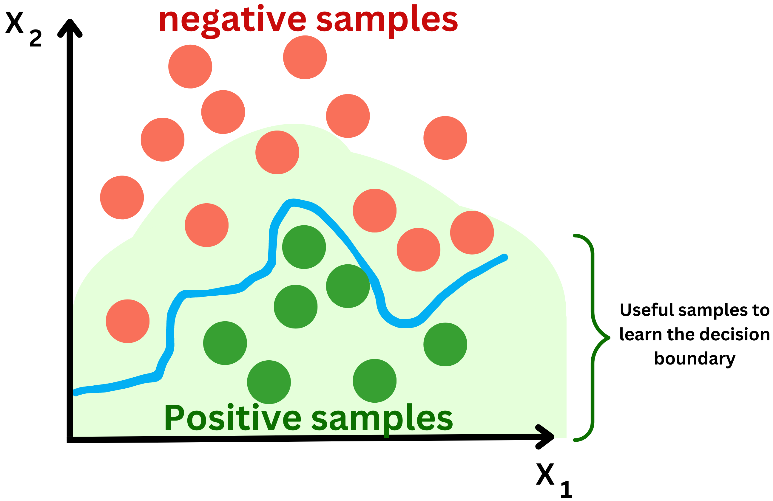
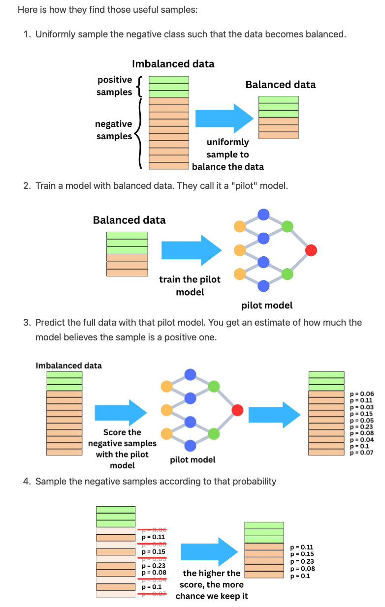
Correcting the probabilities
- In the case of uniform sampling, where all negative samples are equally likely to be selected, the probability estimates can be directly calculated from the data. However, when non-uniform negative sampling is used, the probability estimates based on the downsampled negative samples may not accurately reflect the true probabilities of the original data.
- To address this issue, TikTok uses a technique called probability calibration to correct the probabilities. This involves adjusting the probabilities to reflect the true distribution of the data, so that the model can make accurate predictions.
- For example, if the model assigns a probability of 0.7 to a certain event, it means that it is 70% confident that the event will occur. By calibrating the probabilities, the model can be trained to make more accurate predictions, even when non-uniform negative sampling is used.
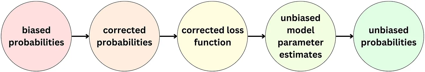
Real time streaming engine for online training
- Recommending on a platform like TikTok is tough because the training data is non-stationary as a user’s interest can change in a matter of minutes and the number of users, videos, and ads keeps changing. The predictive performance of a recommender system on a social media platform deteriorates in a matter of hours so it needs to be updated as often as possible.
-
As a reference, the Ads ranking models at Meta are updated on a daily basis with a recurrent training process.
- Below, we can see the typical process for updating a model is as follows:
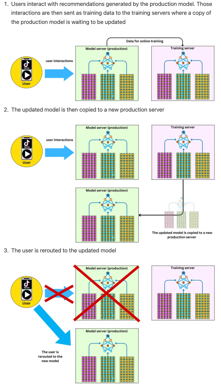
TikTok online training process
- The TikTok recommender models are of the order of ~10 TB in size and it becomes impractical to update often models that large! They realized a few things:
- Most of the model size comes from embedding tables.
- Dense variables move much slower than sparse embeddings.
- Given a short time windows, only a small subset of IDs gets trained and their embeddings updated.
- As a consequence they opted for a partial update of the model. In a specific time window, they know what users interacted with what videos and they are only updating the embedding vectors of those every minute while the whole model is updated daily.
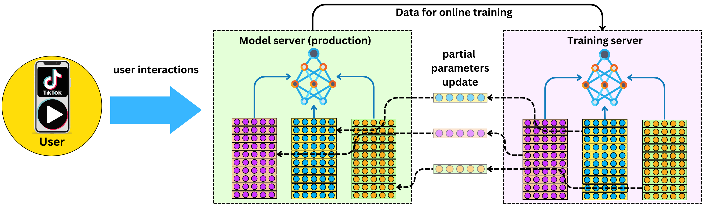
- A partial update means updating only a portion of the model instead of retraining the entire model from scratch. In the case of TikTok’s recommender system, this partial update can be done on the fly, meaning it can be updated in real-time as new user feedback comes in without the need for an additional production server. This allows TikTok to make updates quickly and efficiently, without disrupting the user experience or requiring significant resources.
- The low latency in the model’s ability to update to user feedback is one of the reasons why TikTok’s recommender system is considered one of the most effective in the world at the scale it operates at.
Streaming engine architecture
- TikTok uses a streaming MLOps platform that can efficiently switch between batch training, online training and serving.
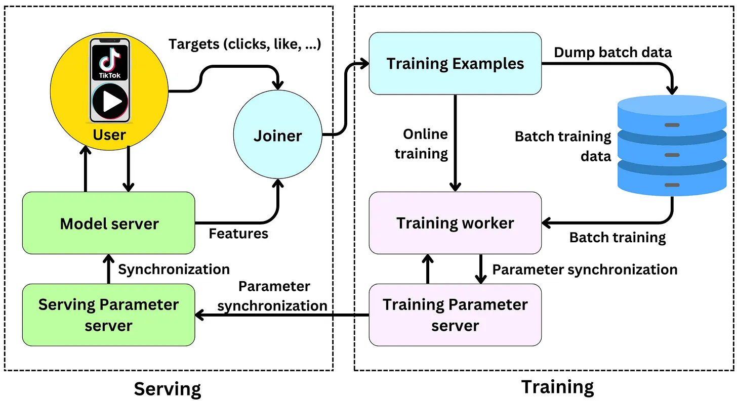
- The production model generates recommendations using the current features.
- The user interacts (clicks, likes, comments, watch the whole video, …) with the production model recommendations which leads to immediate targets that can be used in subsequent training data.
- The Joiner links the features used for generating recommendations and user engagement.
- The resulting data is sent to a database as future training data and to the training worker to be used as current online training data.
- Once the model in the training server is updated, the updated parameters are sent to the serving parameters server and the production model is synchronized with the model in the training server.
- Pinterest uses Transformers to personalize recommendations by encoding short and long term user behaviors.
- “Pins are a combination of an image, text description and an external link to the actual product. Each of the pins is represented by an embedding which is an aggregation of visual, text annotations, and engagement information on that pin.” (source)
- A latent representation is a mathematical representation of a user or item that captures its underlying characteristics or features. In the context of recommender systems, we might use a latent representation to capture a user’s preferences for certain types of items, or an item’s relevance to certain types of users.
- A typical recommender system, we learn a user’s latent representation based on specific training data. However, because the amount of data processed by a platform like Pinterest is so large, it is often the case that the training data for a machine learning model doesn’t span longer than 30 days. This means that the user behavior captured by the model only reflects the last 30 days of user activity. Any behavior that occurred prior to that is forgotten, and the model cannot capture short-term interests that might have emerged within the last hour, for example.
- In typical model development, the problem is framed as a classification problem where we try to predict whether a user will interact with an item or not. However, this approach ignores the intrinsic time-series structure of the problem, which means that the model may not be able to capture the dynamic changes in user behavior over time. In other words, the model may not be able to adapt quickly to changes in user behavior or preferences, which can lead to decreased performance over time.
- “Pinterest goes about that problem differently! They learn long and short term interests separately. They first train the PinnerFormer Transformer (https://lnkd.in/djT-_kt4) by looking at user-pins engagement time series as far back as 1 year from now. The Transformer is able to learn the relationship between different engagements at different points in time in order to predict the future. Instead of predicting only the next engagement, they built a loss function that takes into account all future engagements in the next 14 days. The last attention layer of the model is used as an encoding for long term user interests and captured into a database.” (source)
-
“Another Transformer is trained using the long term user embedding as input and short term past actions (hours or minutes ago) to predict next pin or ad interaction, depending on the ranking problem. It learns the relationship between the different short term actions and long term interest to recommend the items.” (source)
- The image below (source) shows the architecture of Pinterest’s Transformer.
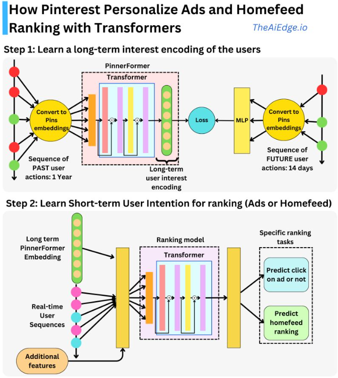
- Now let’s delve deeper into how Pinterest uses Transformers for multimodal Image retrieval.
- Pinterest has been working on a new feature that allows users to search for products or pins using an image as a query and a text prompt to modify the query. In essence, you can share the image and write that you want it in a different color, and it will retrieve it for you!
- Let’s look at how it works:
- First, the images are passing through a visual transformer, something like Swin, which has been trained on ImageNet dataset, which is a large collection of images with annotated labels.
- During training, the network learns to identify and extract important features from the images that are useful for predicting the correct label. The latent representation of an image is generated by taking the output of the last two layers of the visual Transformer and concatenating them together.
- Similarly, the text prompts are processed through a DistilBERT Transformer model. The specific DistilBERT model used here has been trained on two large text datasets: the BooksCorpus and the English Wikipedia corpus. During training, the network learns to predict masked words in a sentence in a self-supervised learning manner. The latent representation of a text prompt is generated by taking the output of the last layer of the DistilBERT model.
- The image and text latent representations are concatenated and used as inputs to a Fastformer transformer to then learn a latent joint image-text representation that is similar to the image we are trying to find.
- Training data: set of image-text prompt pairs as inputs and images as targets.
- E.g.: input: image of a blue top + text prompt
I need it in black.- Target:
picture with same top in black.
- Target:
- “The target image is passed through the same visual transformer described above and the Fastformer is trained trying to maximize the dot product similarity between the image representation and the learned joint image-text representation.” (source)
- The learned joint image-text representations serve as a query in an image database.
- Remember, the joint image-text representations are the latent representations of both images and corresponding textual descriptions, which have been extracted using the visual Transformer and DistilBERT Transformer, respectively. These representations have been learned in a way that allows them to capture the semantic meaning of both the image and the text.
- The searchable images in the database have also been encoded into their own latent representations using the same visual Transformer that was used to extract the latent representations for the query images. These encoded representations are then stored in the database.
-
To retrieve images from the database that are most similar to the query image-text representation, a nearest-neighbor search is performed using the Euclidean distance between the encoded representations. This means that the images with the smallest Euclidean distance from the query representation are returned, as they are the ones that are most similar in terms of their joint image-text representation. These retrieved images are then ordered based on their Euclidean distances from the query representation
- The image below (source) illustrates all the steps mentioned above!
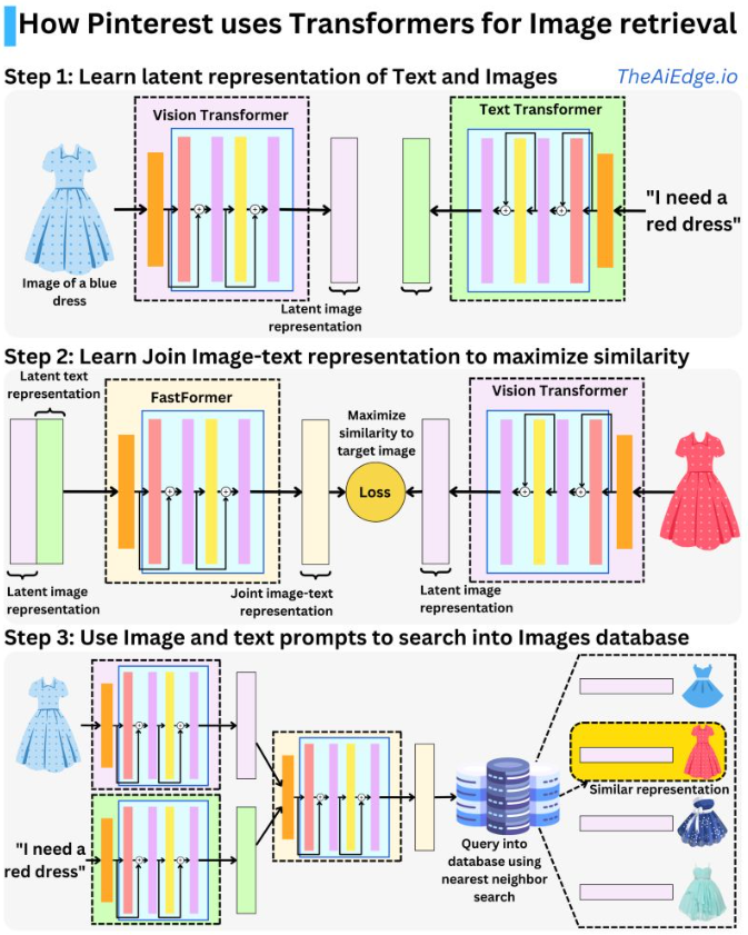
Google Search - by Damien Benveniste, PHD
- link to post
- How would you ARCHITECT a search engine like Google Search? That is a very common Machine Learning System Design interview question. There are more than 50B indexed websites and ~40K searches per second. The system needs to be fast, scalable and needs to adapt to the latest news!
- When a query is created, it goes through a spell check and it is expanded with additional terms such as synonyms to cover as well as possible the user’s query. We know Google uses RankBrain (https://lnkd.in/g4FvNeAT) and it is used only 10% of the time. It is using a word vector representation to find semantically similar words.
- The query is then matched against a database, very likely by keyword matching for very fast retrieval. A large set of documents are then selected. The small subset of those documents is selected using simple (fast) heuristic such as PageRank and other contextual information.
- The ranking process happens in stages. The results go through a set of Recommender engines. There is most likely a simple Recommender Engine first ranking a large amount of documents (maybe 100,000 or 10,000 documents) and a complex one refining the ranking of the top ranked documents (maybe 100 or 1000). At this point, there might be tens of thousands of features created from the different entities at play: the user, the pages, the query, and the context. Google captures the user history, the pages interaction with other users, the pages natural language semantic, the query semantic, … The context relates to the time of the day, day of the week, … but also the current news of the day.
- We will most likely need different model types for different languages, regions, platforms (website, mobile apps, …), document types, … There might be models that specialize in the pure search but I expect there are models that specialize in further filtering such as age appropriate websites or websites containing hate speech.
- A typical server can handle 10,000 HTTP requests per second, but the limiting latency factor is mostly coming from the machine learning models. For example, if ranking 10,000 documents takes ~200 ms, that means we need ~8000 ML servers up at all times to handle the 40K/s requests.
- Because Google is a search engine for multiple types of documents, we have a Universal Search Aggregation system to merge the search results. After the user is served with the results, we can use the user engagement to assess the models in online experiments and aggregate the training data for following model developments and recurrent training processes.
- I guess we could use a tool like ChatGPT to extract a natural language representation of the resulting search results? Let’s see how Bing will handle that pairing!
Fastformer
- Fastformer is a transformer-based architecture for natural language processing (NLP) tasks, developed by researchers at Microsoft Research. It is designed to be faster and more efficient than traditional transformers, while still achieving state-of-the-art results on a range of NLP tasks.
- One of the key innovations of Fastformer is the use of Fast Attention Via positive Orthogonal Random features (FAVOR+), which is a method for approximating the attention mechanism used in transformers. This allows Fastformer to reduce the computational complexity of the attention mechanism while maintaining good performance.
- In addition to being faster, Fastformer also allows for more flexible input formats than traditional transformers. For example, it can handle input sequences of varying lengths and can perform multitask learning with different input modalities, such as text and images.
Pinterest uses Transformers
- Remember, Recommender systems leverage latent representations of users and items to match items to users based on their preferences or characteristics. This matching process typically involves measuring the similarity or compatibility between the latent representations.
- One common approach is collaborative filtering, which utilizes the similarity between users or items to make recommendations. In collaborative filtering, the latent representations of users and items are used to calculate similarity scores. These scores indicate how similar or compatible a user’s preferences or behaviors are to the characteristics of different items.
- For user-based collaborative filtering, the system identifies users with similar latent representations to the target user and recommends items that those similar users have shown interest in. Similarly, for item-based collaborative filtering, the system identifies items that are similar to the ones the user has shown interest in, based on their latent representations.
- Other recommendation techniques, such as matrix factorization and deep learning models, also utilize latent representations to match items to users. These models learn latent factors that capture the relationships between users and items and use these representations to generate recommendations.
How Pinterest Personalizes Ads and Homefeed Ranking with Transformers
- In the context of recommender systems, it is common practice to generate latent representations for both users and items being recommended.
- These latent representations capture underlying characteristics or features of users and items that are relevant for making accurate recommendations. Specifically, when training a recommender system, we aim to learn a user representation that is tailored to the specific training data available. This user representation serves as a condensed and informative representation of the user’s preferences, behaviors, or other relevant attributes, allowing the system to effectively match users with appropriate recommendations.
- Considering the amount of data that a platform like Pinterest sees every day, it is common that the training data for a ML model doesn’t spam longer than 30 days, in which case we learn a user behavior which only captures the last 30 days. Whatever behavior the user had prior to that is forgotten and any short term interests (the past hour let’s say) are not understood by the model.
- In typical model development, the problem is a classification problem where we try to predict if a user will interact with an item or not. We build features to capture past actions but we don’t take into account the intrinsic time-series structure of the problem.
- Pinterest goes about that problem differently! They learn long and short term interests separately. They first train the PinnerFormer Transformer (“PinnerFormer: Sequence Modeling for User Representation at Pinterest“) by looking at user-pins engagement time series back 1 year. The Transformer is able to learn the relationship between different engagements at different points in time in order to predict the future. Instead of predicting only the next engagement, they built a loss function that takes into account all future engagements in the next 14 or 28 days.
- The last attention layer of the model is used as an encoding for long term user interests and captured into a database.
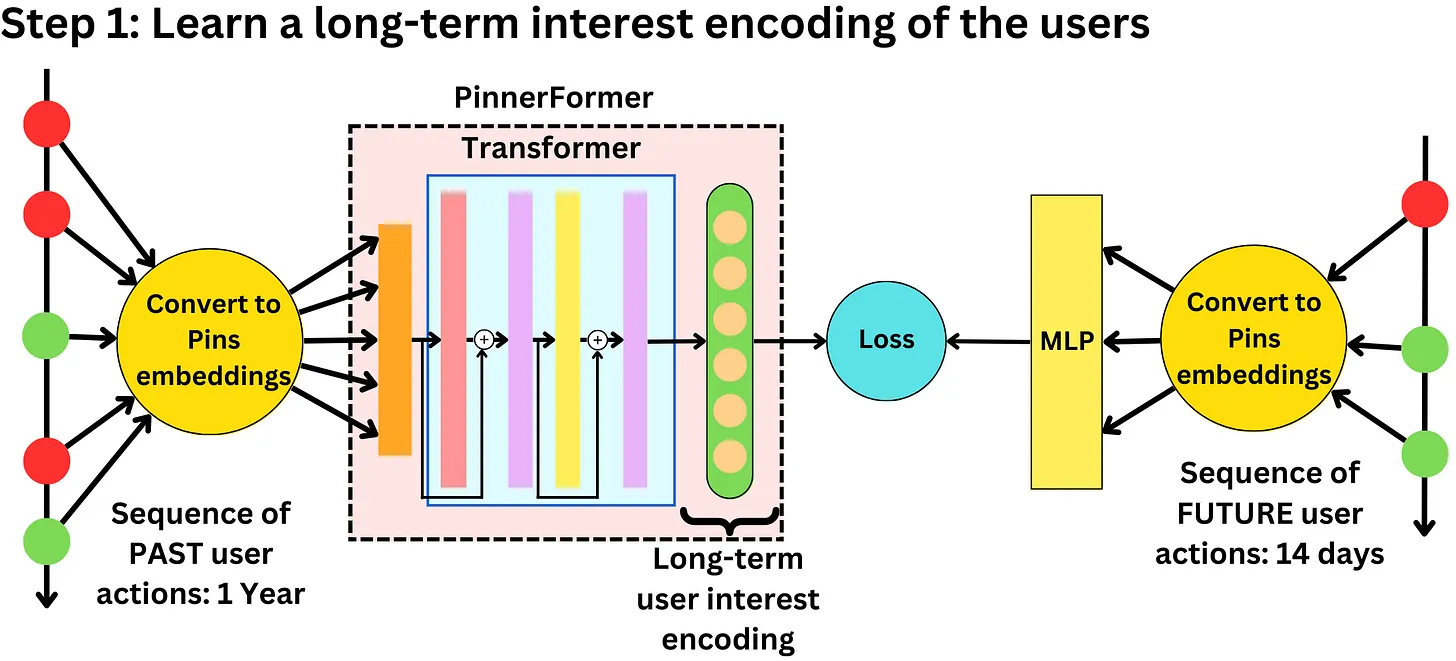
- Depending on the ranking problem, another Transformer uses long-term user embeddings and short-term past actions (hours or minutes ago) to predict next pin or ad interaction. To recommend products to users, the Transformer learns the relationship between short-term actions and long-term interests. Check out the article: “Rethinking Personalized Ranking at Pinterest: An End-to-End Approach“.
PinnerFormer the paper
- PinnerFormer, which is a user representation model trained to predict a user’s future long-term engagement based on their recent actions. Unlike previous methods that focus on predicting the next action, PinnerFormer models the long-term future actions of users using a sequential model. The authors also adapt their modeling to a batch infrastructure and propose a new dense all-action loss. Through extensive offline experimentation and ablations, they demonstrate that PinnerFormer bridges the gap between batch user embeddings generated once a day and real-time user embeddings generated with each user action. The efficacy of PinnerFormer is validated through A/B experiments, showing significant improvements in user retention and engagement compared to the previous user representation model used by Pinterest. As a result, PinnerFormer has been deployed in production since Fall 2021.
- Learning user embeddings (representations) has become an increasingly popular method of improving recommendations. Such embeddings have been adopted to power ranking and candidate generation in industry, and are used to power personalized recommendations across YouTube [6], Google Play [26], Airbnb search[8], J.com search [30], Alibaba [12, 18], and more. In addition to work on learning personalized embeddings, there is a body of work focused on directly building ranking models using sequential information [4, 18, 19, 31], enabling personalization of recommendations based on a user’s recent engagement.
- The use of multiple embeddings in the PinnerSage model was primarily intended for retrieval tasks. By allowing for a variable number of embeddings, the model could more explicitly capture the diverse interests of users. This approach is well-suited for retrieval scenarios where the goal is to find items that align closely with specific user interests or preferences.
- Retrieval tasks involve matching user queries or profiles with relevant items from a large corpus. By generating multiple embeddings, each representing a different aspect of a user’s interests, PinnerSage could enhance the precision and recall of retrieval results. The model could better capture the nuanced preferences of users and facilitate more accurate matching between users and items.
- However, as mentioned in the passage, using multiple embeddings can introduce challenges in terms of scalability, storage requirements, and computational efficiency, especially in downstream models like ranking models. Therefore, for the PinnerFormer model, the authors opted for a single embedding that captures a user’s interests, aiming for simplicity and ease of use in downstream models.
- Prior work on sequential user modeling often focuses on models that operate in real-time or near real-time. However, this approach presents challenges such as high computational costs and increased infrastructure complexity. Real-time models require fetching all events in a user’s history and frequently inferring a potentially complex model for every user action. This results in significant computational resources being utilized and a need for a robust system to handle potential data corruption and recover the model’s state.
- On Pinterest, users may perform tens or hundreds of actions in a single day. Therefore, a model that updates a user’s embedding at most once per day significantly reduces the computational resources required compared to a real-time model of similar scale. By inferring a user’s embedding on a daily basis, the computational cost and infrastructure complexity are significantly reduced.
- In offline evaluations, the authors demonstrate that their loss formulation substantially narrows the performance gap between real-time and daily-inferred models. Additionally, in A/B experiments, PinnerFormer is shown to greatly improve the performance of downstream ranking models. This indicates that the choice to focus on daily inference instead of real-time inference in PinnerFormer leads to improved performance while reducing computational costs and infrastructure complexity.
- Overall, the design choice of employing daily-inferred models in PinnerFormer offers a practical and efficient solution for sequential user modeling in platforms like Pinterest, where users’ actions can be numerous. By minimizing computational resources and leveraging the benefits of offline inference, PinnerFormer achieves competitive performance while streamlining the modeling process.
- The model operates on a corpus of pins and a set of users. Each pin has a PinSage embedding that combines visual, text, and engagement information. Users have a sequence of actions they have taken on the site, such as saves, clicks, reactions, and comments on pins. Actions are represented by PinSage embeddings and metadata. The model aims to learn user representations compatible with pin representations, using cosine similarity.
- To handle the large number of actions, the model computes a user’s embedding using their most recent actions. The objective is to learn embeddings that can predict a user’s positive future engagement with pins over a 14-day window, rather than just the next action. The model focuses on predicting positive engagements such as pin saves, long clickthroughs, and close-ups.
- The primary goal is to learn embeddings that prioritize pins with higher engagement probabilities for each user. The 14-day window is chosen for tractability, assuming that actions taken within this period sufficiently represent a user’s longer-term interests. The architecture of PinnerFormer is illustrated in Figure 1, with each component explained in more detail.
- In PinnerFormer, the focus is on learning user representations rather than pin representations. The embeddings used in PinnerFormer are computed based on the user’s sequence of actions on the site, which include engagements with pins. These user embeddings capture the user’s interests and preferences based on their past actions and interactions with pins.
- While PinSage embeddings are specific to individual pins, the embeddings in PinnerFormer represent the users and their aggregated preferences. The goal is to learn user embeddings that are compatible with pin embeddings under cosine similarity, enabling the model to predict a user’s future engagement with pins.
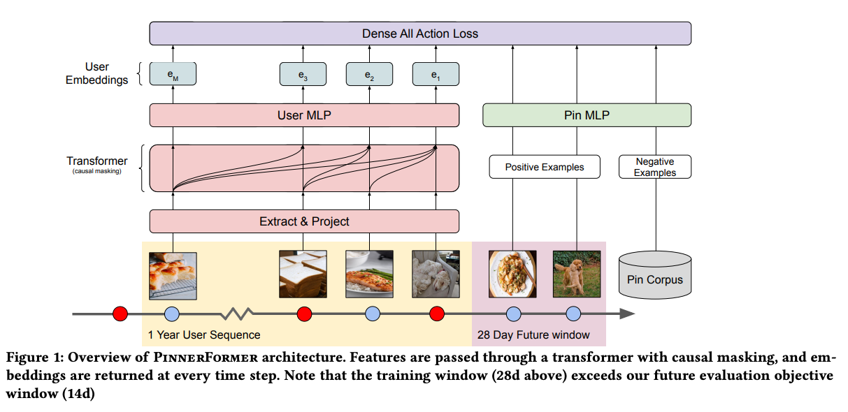
- To construct the transformer input, we utilized three important realtime user sequence features:
- Engaged pin embedding: pin embeddings (learned GraphSage embedding) for the past 100 engaged pins in user history
- Action type: type of engagement in user action sequence (e.g., repin, click, hide)
- Timestamp: timestamp of a user’s engagement in user history
- We also use candidate pin embedding to perform early fusion with the above realtime user sequence features.
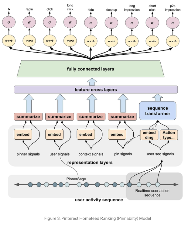
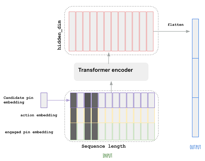
- As illustrated in Figure 3, to construct the input of the sequence transformer module, we stack the [candidate_pin_emb, action_emb, engaged_pin_emb] to a matrix. The early fusion of candidate pin and user sequence is proved to be very important according to online and offline experiments. We also apply a random time window mask on entries in the sequence where the actions were taken within one day of request time. The random time window mask is used to make the model less responsive and to avoid diversity drop. Then we feed it into a transformer encoder. For the initial experiment, we only use one transformer encoder layer. The output of the transformer encoder is a matrix of shape [seq_len, hidden_dim]. We then flatten the output to a vector and feed it along with all other features to MLP layers to predict multi-head user actions.
- In our second iteration of the user sequence module (v1.1), we made some tuning on top of the v1.0 architecture. We increased the number of transformer encoder layers and compressed the transformer output. Instead of flattening the full output matrix, we only took the first 10 output tokens, concatenated them with the max pooling token, and flattened it to a vector of length (10 + 1) * hidden_dim. The first 10 output tokens capture the user’s most recent interests and the max pooling token can represent the user’s longer term preference. Because the output size became much smaller, it’s affordable to apply an explicit feature crossing layer with DCN v2 architecture on the full feature set as previously illustrated in Fig.2.
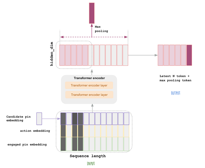
- Offline Evaluation
-
We perform offline evaluation on different models that process realtime user sequence features. Specifically, we tried the following architectures:
- Average Pooling: the simplest architecture where we use the average of pin embedding in user sequence to present user’s short term interest
- (Convolutional Neural Network (CNN): uses CNN to encoder a sequence of pin embedding. CNN is suitable to capture the dependent relationship across local information
- Recurrent Neural Network (RNN): uses RNN to encoder a sequence of pin embedding. Compared to CNN, RNN better captures longer term dependencies.
- Lost Short-Term Memory (LSTM): uses LSTM, a more sophisticated version of RNN that captures longer-term dependencies even better than RNN by using memory cells and gating.
- Vanilla Transformer: encodes only the pin embedding sequence directly using the Transformer module.
- Improved Transformer v1.0: Improved transformer architecture as illustrated in Figure 4.
-
For Homefeed surface specifically, two of the most important metrics are HIT@3 for repin and hide prediction. For repin, we try to improve the HIT@3. For hide, the goal is to decrease HIT@3.
-
The offline result shows us that even with the vanilla transformer and only pin embeddings, the performance is already better than other architectures. The improved transformer architecture showed very strong offline results: +8.87% offline repin and a -13.49% hide drop. The gain of improved transformer 1.0 from vanilla transformer came from several aspects:
- Using action embedding: this helps model distinguish positive and negative engagement
- Early fusion of candidate pin and user sequence: this contributes to the majority of engagement gain, according to online and offline experiment,
- Random time window mask: helps with diversity
- Online Evaluation
- Then we conducted an online A/B experiment on 1.5% of the total traffic with the improved transformer model v1.0. During the online experiment, we observed that the repin volume for overall users increased by 6%. We define the set of new, casual, and resurrected users as non-core users. And we observed that the repin volume gain on non-core users can reach 11%. Aligning with offline evaluation, the hide volume was decreased by 10%.
-
Recently, we tried transformer model v1.1 as illustrated in Figure 4, and we achieved an additional 5% repin gain on top of the v1.0 model. Hide volume remains neutral for v1.0.
- Architecture:
- The model architecture used in PinnerFormer is based on a transformer model, which has been widely successful in various natural language processing tasks. The transformer model is utilized to model the sequence of user actions.
- To represent the user’s sequence of actions, an input matrix is constructed, where each row corresponds to an action and the columns represent the input dimensions. The input matrix is then projected to the hidden dimension of the transformer, and positional encoding is added. The transformer consists of alternating feedforward network (FFN) and multi-head self-attention (MHSA) blocks, which allow the model to capture dependencies and patterns in the user’s action sequence.
- The output of the transformer at each position is passed through a small multi-layer perceptron (MLP) and normalized using L2 normalization, resulting in a set of user embeddings. These embeddings capture the user’s preferences and interests based on their past actions.
- For representing pins, a separate MLP is trained using PinSage embeddings as input, and the output embeddings are also normalized using L2 normalization. This ensures consistency in the representation of both users and pins, leading to stable training and preserving offline performance.
- By utilizing the transformer model and normalized embeddings, PinnerFormer is able to effectively model the user’s sequence of actions and represent both users and pins in a consistent manner, facilitating accurate prediction of user engagement with pins.
How Pinterest uses Transformers for image retrieval
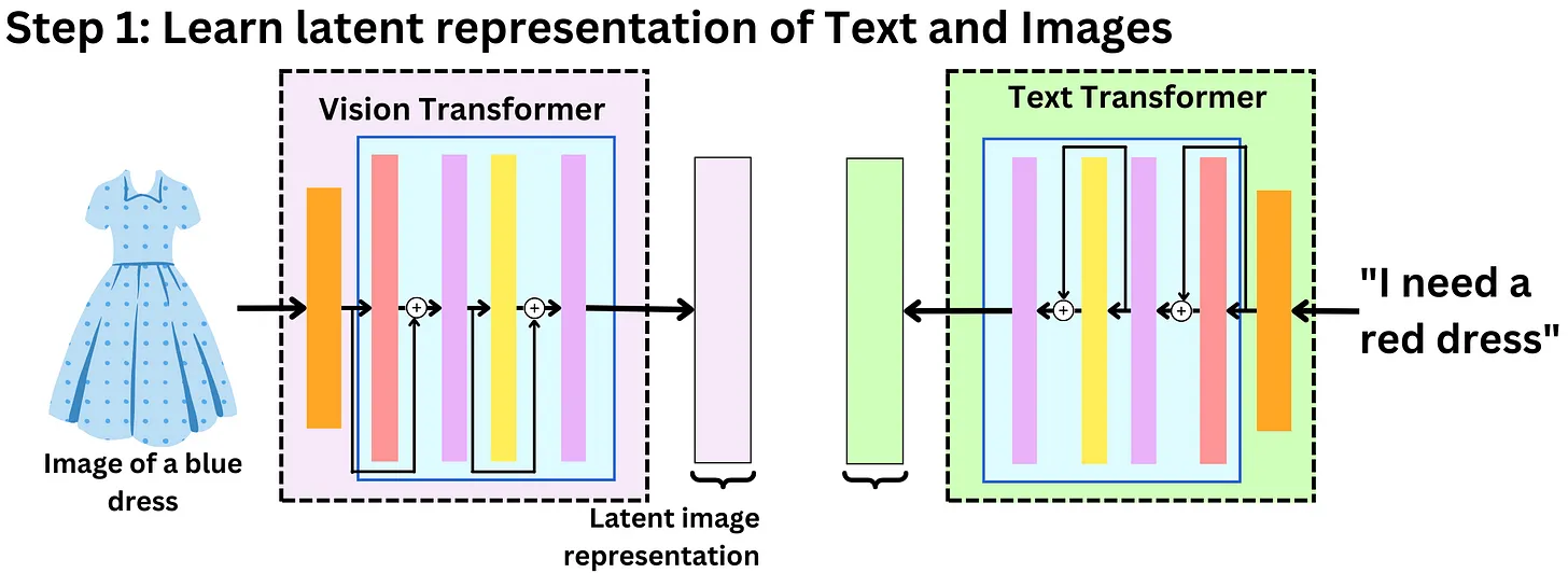
- Pinterest has been working on a new feature that allows users to search for products or pins using an image as a query and a text prompt to modify the query (“Fashion Image Retrieval with Text Feedback by Additive Attention Compositional Learning“). Imagine taking a picture of a blue dress and writing “I need it red and longer” and being recommended a set of dresses that fit the description! Pretty cool! Here is how to build such a retrieval system with Transformers:
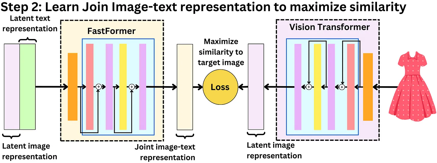
- Pinterest developed a system of a retrieval using transformers for image search with text feedback. The process involves several steps:
- Latent Representations: Images are processed using a visual transformer, while text prompts go through a DistilBERT transformer to obtain their latent representations.
- Concatenation: The latent representations of images and text are concatenated to create joint image-text representations.
- Joint Representation Learning: A Fastformer transformer is employed to learn a latent joint image-text representation by training on pairs of image-text prompts and corresponding target images. The objective is to maximize the similarity between the image representation and the learned joint representation.
- Image Database: The searchable images are encoded into latent representations and stored in a database.
- Retrieval: Nearest-neighbor search is performed using the joint image-text representation as a query, and the images in the database are retrieved based on their Euclidean distances from the query representation.
- The approach demonstrates the use of multiple ML models as building blocks to create a smart retrieval system. It highlights the potential of combining different models to build more sophisticated and useful products. The author anticipates a future where smart products will rely on software and ML models working together on a larger scale.
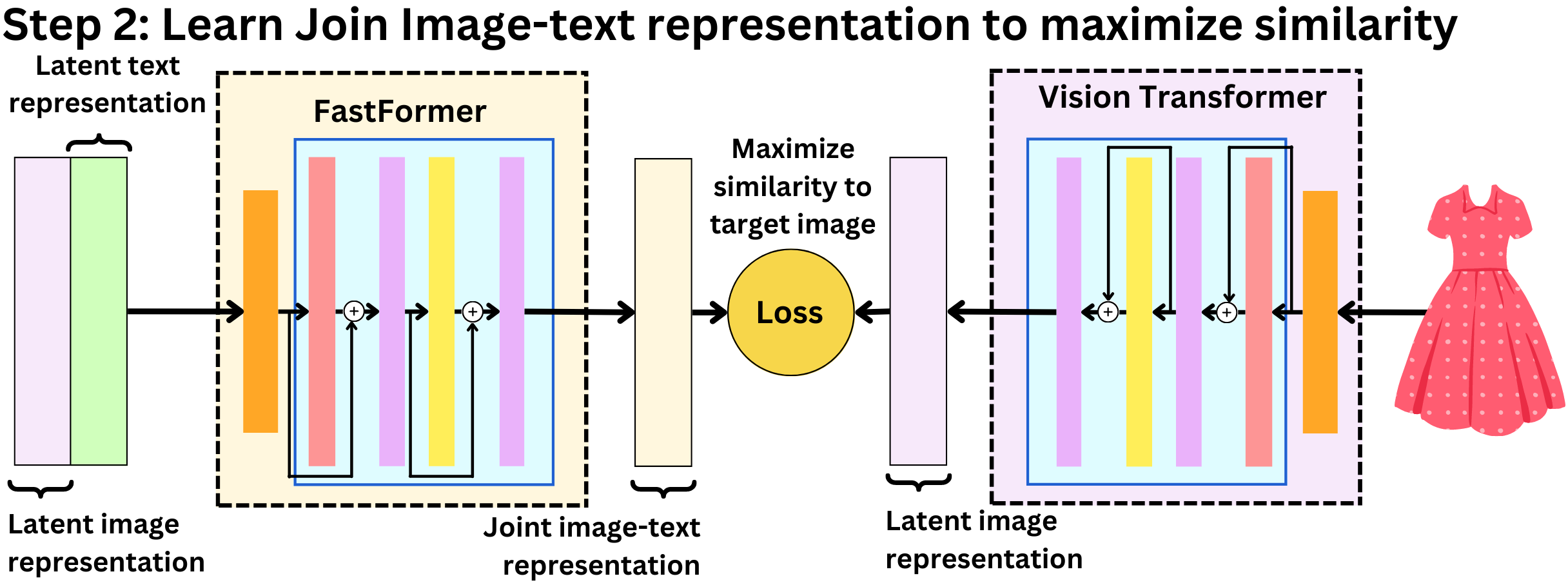
Overview of current systems from Eugene Yan
- The list below has been inspired from Eugene Yan’s blog.
Alibab
- Below, we describes Alibaba’s design for candidate retrieval and ranking in Taobao, their e-commerce platform. Here’s a breakdown of the process:
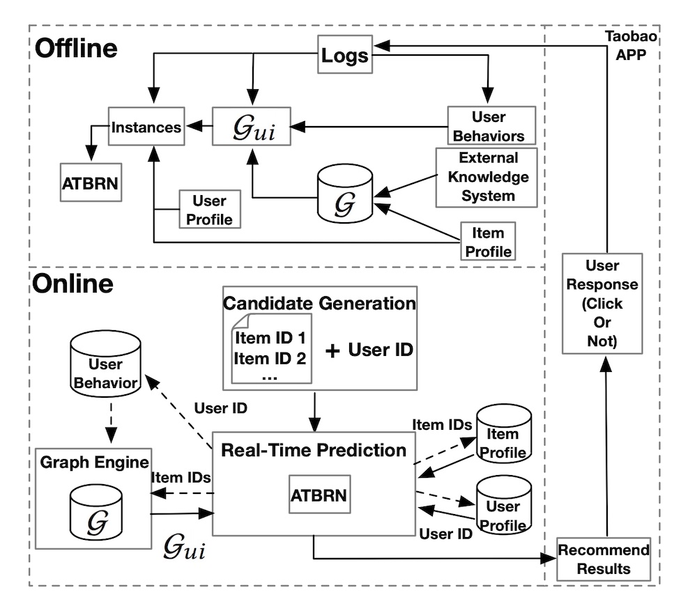
Candidate Retrieval:
- Offline Environment: In the offline environment, user-item interactions at the session level are analyzed to create a weighted, bidirectional item graph. This graph serves as the basis for generating item sequences through random walks.
- Item Embeddings: Item embeddings are learned using representation learning techniques like word2vec skip-gram. This allows the system to generate numerical representations of items without relying on explicit labels.
- Item-to-Item Similarity Map: The learned item embeddings are used to find the nearest neighbors for each item. These neighbors are then stored in an item-to-item similarity map, acting as a key-value store.
Online Environment:
- User Interaction: When a user launches the Taobao app, the Taobao Personalization Platform (TPP) fetches the latest items that the user has interacted with (such as clicking, liking, or purchasing).
- Candidate Retrieval: The items retrieved from user interactions are used to retrieve candidate items from the item-to-item similarity map created in the offline environment.
- Ranking: The retrieved candidates are passed to the Ranking Service Platform (RSP), where a deep neural network is employed for ranking. The network considers various factors and features to determine the most relevant and personalized items for the user.
- Display to the User: The ranked candidate items are then displayed to the user, tailored to their preferences and behavior.
Ranking:
- Offline Environment: In the offline environment, Alibaba combines an existing knowledge graph, user behavior information, and item data to create an adaptive knowledge graph called G_ui.
- Adaptive Target-Behavior Relational Graph Network (ATBRN): The adaptive knowledge graph (G_ui) is merged with user data like demographics and user-item preferences to train the ranking model known as ATBRN. This graph network considers the relationships between different entities and attributes to generate more accurate rankings.
- Online Environment: When a user request is received, the candidate generator retrieves a set of candidates based on the user ID. The Real-Time Prediction (RTP) platform then queries the knowledge graph and feature stores to gather relevant item and user attributes.
- Ranking Prediction: The retrieved graph representations, along with item and user data, are fed into the ATBRN ranking model. The model predicts the probability of a user clicking on each candidate item.
- Reordering and Display: The candidate items are reordered based on the predicted probabilities, and the updated ranking is displayed to the user, optimizing the likelihood of relevant items being seen and engaged with.
Alibaba employs techniques like item embeddings and item-to-item similarity maps for candidate retrieval, while using deep neural networks and graph networks like ATBRN for ranking in their Taobao platform. The system combines offline analysis of user-item interactions with online user requests to provide personalized and relevant item recommendations to users.
- Below, we describes Facebook’s design for embedding-based retrieval in their search system. Here’s a breakdown of the process:
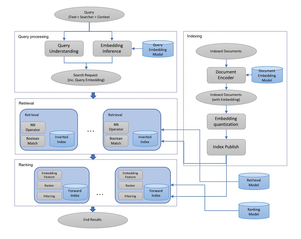
Offline Environment:
-
Two-Tower Network: In the offline environment, Facebook trains a two-tower network consisting of a query encoder and a document encoder. This network is designed to output cosine similarity scores for each query-document pair. The query encoder and document encoder ensure that search queries and documents (such as user profiles or groups) are embedded into the same vector space.
-
Document Embedding: Using the document encoder, Facebook embeds each document using Spark batch jobs. The embeddings capture the semantic representation of the document. These embeddings are then quantized, which means they are transformed into a lower-dimensional representation to optimize storage and retrieval efficiency.
-
ANN Index and Forward Index: The quantized document embeddings are published into an approximate nearest neighbor (ANN) index, often referred to as an “inverted index.” This index is based on Faiss, a library for efficient similarity search and clustering of dense vectors. Additionally, the embeddings are also published in a forward index without quantization. The forward index can include other relevant data, such as profile and group attributes, to augment candidate selection during the ranking process.
Online Environment:
-
Query Encoding: In the online environment, each search request undergoes query understanding, and the query is embedded using the query encoder. This process captures the semantic representation of the search query.
-
Retrieval Step: The embedded search request is then used to retrieve nearest neighbor candidates from the ANN index. The ANN index efficiently identifies documents that are most similar to the query based on their embeddings. Additionally, boolean filtering can be applied to further refine the candidates based on specific criteria such as name matching or location matching.
-
Candidate Augmentation: The retrieved candidates are augmented with their full embeddings from the forward index. This ensures that additional information and attributes associated with the documents, such as profile and group data, are included.
-
Ranking: The augmented candidates, along with their complete embeddings and additional data, undergo the ranking process. Facebook’s ranking algorithm considers various factors and features to determine the most relevant and personalized order of the candidates.
- Facebook’s embedding-based retrieval system involves training a two-tower network, embedding documents using batch jobs, building an ANN index for efficient retrieval, and augmenting candidates with additional data. In the online environment, queries are encoded, candidates are retrieved using the ANN index, and the ranking process takes place considering the augmented candidates and their embeddings. This approach enables Facebook to provide accurate and relevant search results to users based on semantic similarity between queries and documents.
JD
- Below is JD’s approach to semantic retrieval for search in an e-commerce system. Here’s an explanation of the key points:
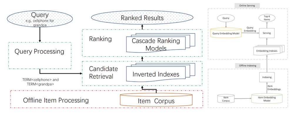
 Offline Environment:
- Two-Tower Model: In the offline environment, JD trains a two-tower model with a query encoder and an item encoder. This model is designed to output a similarity score for each query-item pair, capturing the semantic relationship between them.
- Item Embedding: The item encoder embeds catalog items, representing them in a numerical vector space. These embeddings are generated to facilitate efficient retrieval.
- Embedding Index: The embeddings are loaded into an embedding index, which is essentially a key-value store. This index allows fast retrieval of items based on their embeddings.
Online Environment:
- Query Preprocessing: In the online environment, each query undergoes preprocessing steps such as spelling correction, tokenization, expansion, and rewriting to enhance the quality of the query.
- Query Embedding: The preprocessed query is embedded using the query encoder, producing a numerical representation that captures its semantic meaning.
- Candidate Retrieval: The query embedding is then used to retrieve candidate items from the embedding index through a nearest neighbors lookup. This step efficiently identifies items that are most similar to the query.
- Ranking: The retrieved candidates are ranked based on factors such as relevance, predicted conversion, etc., to determine their order in the search results.
Optimization Tips:
- Model Training: JD optimized model training by addressing the duplicative nature of user-item interaction, item data, and user data in the input. They built a custom TensorFlow dataset where user and item data are loaded into memory as lookup dictionaries. During training, these dictionaries are queried to append user and item attributes to the training set, reducing the training data size significantly.
- Offline Training and Online Serving Consistency: JD emphasized the importance of consistency between offline training and online serving. They specifically highlighted the tokenization step, which was performed three times (data preprocessing, training, serving). To minimize inconsistencies and skew, they developed a C++ tokenizer with a Python wrapper that was used for all tokenization tasks.
- Model Serving: JD reduced latency by combining services in the model serving phase. Instead of having separate services for query embedding and ANN lookup, they unified these steps in a single instance. This reduced network latency by passing the query embedding to the ANN via memory.
- Multiple Models and Versioning: JD runs multiple models simultaneously for different retrieval tasks and A/B tests. Each model or “servable” consists of a query embedding model and an ANN lookup. These servables are hosted in separate instances, and a proxy module or load balancer is used to direct incoming requests to the appropriate servable based on versioning, deployments, and A/B testing.
Overall, JD’s approach involves training a two-tower model, embedding items, and using an embedding index for candidate retrieval. They employ various optimizations to improve efficiency, consistency, and scalability in both model training and serving stages.
DoorDash
- Next, we move from the embedding + ANN paradigm and look at DoorDash’s use of a knowledge graph for query expansion and retrieval. In the offline environment, they train models for query understanding, query expansion, and ranking. They also load documents (i.e., restaurants and food items) into ElasticSearch for use in retrieval, and attribute data (e.g., ratings, price points, tags) into a feature store.
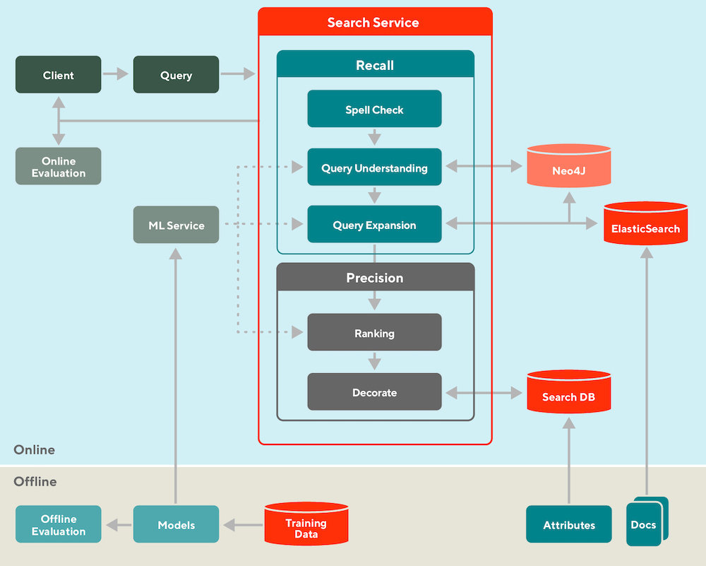
-
How DoorDash splits their search into offline and online, and retrieval (recall) and ranking (precision)
-
DoorDash splits search into offline and online, and retrieval (recall) and ranking (precision).
-
In the online environment, each incoming query is first standardized (e.g., spell check) and synonymized (via a manually curated dictionary). Then, the knowledge graph (Neo4J) expands the query by finding related tags. For example, a query for “KFC” will return tags such as “fried chicken” and “wings”. These tags are then used to retrieve similar restaurants such as “Popeyes” and “Bonchon”.
- These candidates are then ranked based on lexical similarity between the query and documents (aka restaurants, food items), store popularity, and possibly the search context (e.g., time of day, location). Finally, the ranked results are augmented with attributes such as ratings, price point, and delivery time and cost before displayed to the customer.
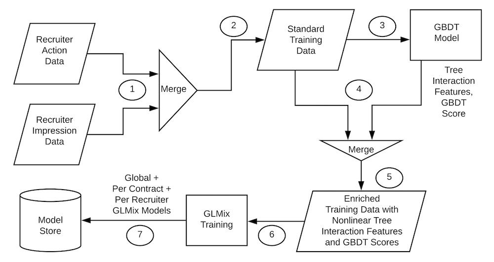
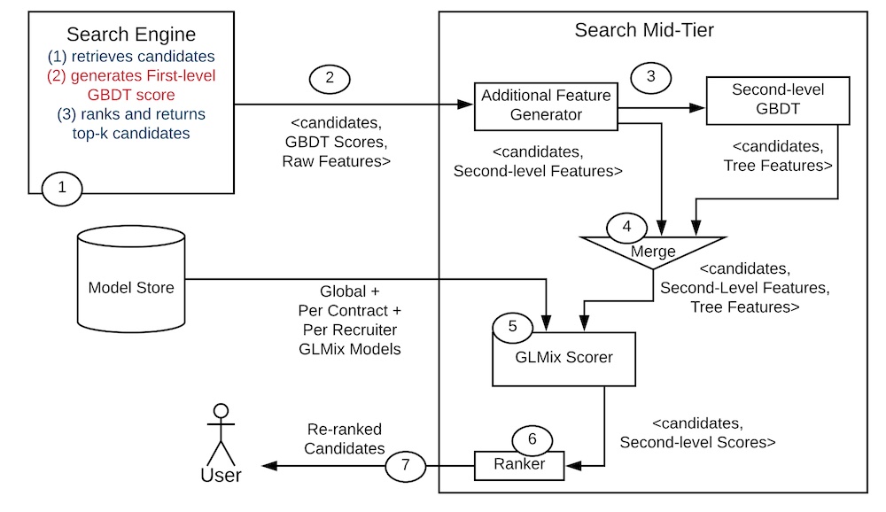 The provided text discusses how LinkedIn personalizes talent search results using XGBoost, a gradient boosting algorithm. Here’s an explanation of the key points:
Offline Environment:
- Training Data Generation: In the offline environment, LinkedIn combines impression and label data to create training data. The labels indicate instances where recruiters sent messages to potential candidates, and the candidates responded positively.
- XGBoost for Feature Generation: The training data is then fed into a pre-trained XGBoost model, which generates model scores and tree interaction features. These features are used to augment the training data, providing additional information for the subsequent ranking model.
- Ranking Model Training: The augmented training data is used to train the ranking model, which in this case is a generalized linear mixed model (GLMix). The ranking model learns to predict the relevance or suitability of candidates for a given search query.
Online Environment:
- Candidate Retrieval: In the online environment, when a search request is received, the search engine (such as Elastic or Solr) retrieves a set of candidates based on the query. These candidates are potential matches for the search query.
- First-level XGBoost Scoring: The retrieved candidates are scored using a first-level XGBoost model. This model helps identify the most promising candidates among the retrieved set.
- Feature Augmentation: The top 1,000 candidates from the previous step are augmented with additional features, which could include information about the candidate, the search query, or other relevant factors.
- Second-level XGBoost for Tree Interactions: The augmented candidates undergo another scoring step using a second-level XGBoost model. This model specifically focuses on capturing interactions between the features and the decision trees of XGBoost.
- Ranking: The augmented candidates are ranked based on their scores, taking into account the XGBoost model outputs and the features generated. The top 125 candidates are then selected for display as search results to the user.
Conclusion: The text concludes by mentioning the common design pattern of offline-online retrieval-ranking systems for search and recommendations. It suggests starting with candidate retrieval using simple embeddings and approximate nearest neighbors, and gradually incorporating a ranker on top. Additionally, it highlights the importance of considering whether real-time retrieval and ranking are necessary or if batch recommendations would suffice, depending on the specific requirements of the system.
Overall, LinkedIn leverages XGBoost for candidate retrieval, feature generation, and ranking to personalize talent search results on their platform.
Batch vs Real- time
- Most use cases don’t require real-time recommendations: In many situations, batch recommendations are sufficient and offer computational advantages. They are generated once a day, benefit from batch processing efficiencies, and can be served through a key-value store.
- Computation and serving decoupling: Batch recommendations can be pre-computed and cached in a key-value store, allowing separation between computation and serving. Even if the compute step fails, the previous batch of slightly stale recommendations can continue to be served, ensuring high uptime and reducing operational burden.
- More computation for real-time recommendations: Real-time recommendations involve aggregating streamed events and generating recommendations on-demand based on user interactions. This requires additional computation compared to batch recommendations, which compute a single set daily. However, recommendations can be saved for customers who don’t visit the app, reducing unnecessary computations.
- Operational challenges for real-time recommendations: Operating real-time recommendations in production is more complex. It requires low-latency high-throughput APIs and continuous uptime. There is no buffer like a key-value store, and the line between compute and serving becomes blurred. This increases the operational burden and may lead to being paged for outages in different time zones.
- While real-time recommendations offer immediate insights, they come with increased computational and operational complexities. For many cases, batch recommendations are sufficient and provide computational advantages and operational stability.
- “Operating real-time recommendations in production is also far tricker. Instead of using ephemeral Spark clusters (for compute) and a DynamoDB (for serving), we’ll need low-latency high-throughput APIs with 24/7 uptime.” (source)
- Real-time recommendations are valuable in situations where the customer journey is mission-centric and time-sensitive. They are particularly useful when the context of the customer’s interaction plays a crucial role. Two examples, shopping and watching a movie, can help illustrate this.
- In shopping, customers often have specific missions in mind. While they may typically purchase products from a specific category, their behavior can be interrupted by time-sensitive missions related to other categories. For instance, if a customer usually shops for clothes but suddenly starts searching for a wide-screen monitor, it becomes essential to update the recommendations promptly to assist the customer in fulfilling their mission. Delayed batch recommendations are not sufficient in such cases. Furthermore, even when batch recommendations are eventually updated, they may not effectively address the immediate needs arising from these time-sensitive missions due to data imbalances.
- Therefore, real-time recommendations are necessary to adapt quickly to the evolving context of the customer and cater to their immediate needs. This helps prevent customers from losing interest or turning to competing platforms to fulfill their missions in a timely manner.
- The movies we choose to watch are influenced by various contextual factors, such as our social situation, mood, and time of day. For example, we may prefer different movies when we are alone, with friends, with a romantic partner, or with children. These contextual factors play a significant role in shaping our movie preferences, and daily batch recommendations struggle to address these dynamic needs effectively.
- In addition to shopping, there are other domains where real-time recommendations prove beneficial. In the travel industry, our vacation destinations often change, and real-time recommendations can help us discover new and relevant options based on our evolving preferences. Platforms like YouTube cater to diverse interests, and within a single day, we may watch videos related to coding, yoga, and recipes. Real-time recommendations can adapt to our changing interests and serve us with relevant content in the moment. Furthermore, in advertising, our interests and attention spans are time-sensitive, requiring real-time recommendations to deliver targeted and engaging ads.
- Real-time recommendations are particularly valuable in scenarios where a large portion of the customer base is new, leading to a cold-start problem. This occurs when a product is newly launched or enters a new market. For instance, when you download a new e-commerce app, the platform may not have enough information about your preferences initially. However, by analyzing your early interactions, such as clicking on a specific item, the platform can quickly infer your preferences and personalize your shopping experience. The recommendations on your home page can then be tailored to your gender, optimizing the relevance of the suggested products.
- Considering that a significant number of users abandon mobile apps after just one use, the ability to respond quickly to customer needs right from the first touchpoint becomes crucial for user acquisition and retention. Real-time recommendations play a vital role in creating a personalized and engaging experience from the outset, enhancing the chances of acquiring and retaining customers.
Fresh Content Needs More Attention: Multi-funnel Fresh Content Recommendation
- High level summary by (source)
- Problem:
- New content faces obstacles in reaching the right users due to limited exposure.
- This is called the cold start problem.
Goal:
- High-quality new content to be surfaced and go viral as well.
- Balance coverage and relevance of content.
- Position new content with the rest of the recommendation stack.
Solution:
- Fresh content nominator
- Users are represented based on consumption history.
- Items are represented based on features.
- Candidates are generated with a fast dot product.
- Graduation filter
- As new content gets interactions, it is picked by the main recommendation system.
- Ranking
- Generate the top 10 candidates with a low-latency multi-armed bandit.
- Top 1 is generated by a DNN with better accuracy but higher latency.

- “Recommendation systems are heavily relied upon to connect users to the right contents on recommendation platforms. Many of these systems are trained on interaction logs collecting historical user interactions with recommended contents. These interactions how- ever are conditioned on the contents these systems chose to expose to users, which creates a strong feedback loop [7] resulting in “rich gets richer” effect. “paper
- It utilizes a two-tower content-based recommendation model, where one tower learns user representations and the other learns item representations based on features. The model is trained to predict user interactions using historical data and can generalize to items with minimal user interactions. During serving, a multiscale quantization technique is employed for efficient retrieval of the top fresh candidates.
- Next, they imply the “Graduation filter” which is a strategy used to handle fresh contents once they have gathered initial interactions. Instead of continuously exploring these items in a dedicated slot, the graduation filter removes contents that have been consumed by users a certain number of times (at least 𝑛 times in this case). This helps save impression resources and allows for their reallocation to other potential fresh and tail contents.
- After passing through the filter, the nominated candidates are ranked using two components: a real-time pre-scorer and a ranker shared with the main system. The lightweight pre-scorer reacts to users’ early feedback in real-time and selects the top-10 candidates. These candidates then undergo assessment by the ranker, which is a deep neural network with higher accuracy but longer latency. The ranker determines the relevance of the selected candidates and returns the top-1 recommendation.
- The pre-scorer implements a real-time Bernoulli multi-arm bandit, where each arm corresponds to a content. The reward of each arm estimates the click-through rate of a fresh content, conditioned on users spending at least 10 seconds after the click. The reward follows a Beta posterior distribution, which is updated based on the interactions and impressions of each arm in real-time. The global prior parameters are estimated through maximum likelihood on fresh items with sufficient impressions.
- At serving time, Thompson Sampling is used to generate a sampled reward for each candidate, and the top-10 candidates with the highest rewards are returned, with the final candidate determined by the ranker.

- “Hybrid Recommendation Systems. In practice, it is impossible to find one model that can obtain the optimal performance in all the scenarios [1, 32]. Serving two or more recommenders simul- taneously to take advantages of the strengths of each is widely adopted [5]. Given that collaborative methods are more powerful when abundant data is available and content-based recommenda- tion works better on cold-start items, there are previous discussions on a hybrid setup of combining content-based filtering with col- laborative filtering to enable to system to serve both the new and existing users [15, 16, 26]. Early hybridization techniques usually compute a linear combination of individual output scores to blend the results from different recommenders [14]. With the recent ad- vance in meta-learning, [11, 12, 32] propose to meta-learn the hard or soft model selector for the optimal hybridization. Meanwhile, the idea of hybrid recommender systems also have a strong connection to the field of ensemble analysis. In this line of work, instead of com- bining different recommendation backbones (e.g., content-based method and collaborative filtering), the systems serve multiple mod- els with the same backbone simultaneously [38, 52]. We here take advantage of both the generalization and real-time models in a multi-funnel setup for fresh recommendation.”