Distilled • Search Engine RecSys Design
- Problem statement
- Metrics
- Architectural Components
- Training Data Generation
- Online Experimentation
- Runtime newsfeed generation
- Practical Tips
- Further Reading
Problem statement
Metrics
-
Choosing a metric for a machine learning model is of paramount importance. Machine learning models learn directly from the data, and no human intuition is encoded into the model. Hence, selecting the wrong metric results in the model becoming optimized for a completely wrong criterion.
- There are two types of metrics to evaluate the success of a search query:
- Online metrics
- Offline metrics
- We refer to metrics that are computed as part of user interaction in a live system as Online metrics. Meanwhile, offline metrics use offline data to measure the quality of your search engine and don’t rely on getting direct feedback from the users of the system.
Offline metrics
- The offline methods to measure a successful search session makes use of trained human raters. They are asked to rate the relevance of the query results objectively, keeping in view well-defined guidelines. These ratings are then aggregated across a query sample to serve as the ground truth.
Ground truth refers to the actual output that is desired of the system. In this case, it is the ranking or rating information provided by the human raters.
- Let’s see normalized discounted cumulative gain (NDCG) in detail as it’s a critical evaluation metric for any ranking problem.
NDCG
- You will be looking at NDCG as a common measure of the quality of search ranking results.
-
NDCG is an improvement on cumulative gain (CG).
\[CG_{p}=\sum_{i=1}^{p} \operatorname{rel}_{i}\]- where, \(rel\) is the relevance rating of a document, \(i\) is the position of the document, and \(p\) is the position up to which the documents are ranked.
Example
-
Let’s look at this concept using an example.
-
A search engine answers a query with the documents \(D_1\) to \(D_4\). It ranks them in the following order of decreasing relevance, i.e., \(D_1\) is the highest-ranked and \(D_4\) is the lowest-ranked:
-
Ranking by search engine: \(D_{1},D_{2},D_{3},D_{4}\)
-
A human rater is shown this result and asked to judge the relevance of each document for the query on a scale of \(0-3\) (\(3\) indicating highly relevant). They rank the documents as follows:
-
The cumulative gain for the search engine’s result ranking is computed by simply adding each document’s relevance rating provided by the human rater.
- In contrast to cumulative gain, discounted cumulative gain (DCG) allows us to penalize the search engine’s ranking if highly relevant documents (as per ground truth) appear lower in the result list.
\[D C G_{p}=\sum_{i=1}^{p} \frac{r e l_{i}}{\log _{2}(i+1)}\]DCG discounts are based on the position of the document in human-rated data. The intuition behind it is that the search engine will not be of much use if it doesn’t show the most relevant documents at the top of search result pages. For example, showing starbucks.com at a lower position for the query “Starbucks”, would not be very useful.
- DCG for the search engine’s ranking is calculated as follows:
-
In the above calculation, you can observe that the denominator penalizes the search engine’s ranking of \(D_{3}\) for appearing later in the list. It was a more relevant document relative to \(D_2\) and should have appeared earlier in the search engine’s ranking.
-
However, DCG can’t be used to compare the search engine’s performance across different queries on an absolute scale. The is because the length of the result list varies from query to query. So, the DCG for a query with a longer result list may be higher due to its length instead of its quality. To remedy this, you need to move towards NDCG.
-
NDCG normalizes the DCG in the 0 to 1 score range by dividing the DCG by the max DCG or the IDCG (ideal discounted cumulative gain) of the query. IDCG is the DCG of an ideal ordering of the search engine’s result list (you’ll see more on IDCG later).
-
NDCG is computed as follows:
-
In order to compute IDCG, you find an ideal ordering of the search engine’s result list. This is done by rearranging the search engine’s results based on the ranking provided by the human raters, as shown below.
-
Now let’s calculate the DCG of the ideal ordering (also known as the IDCG) as shown below:
- Now, let’s finally compute the NDCG:
-
An NDCG value near one indicates good performance by the search engine. Whereas, a value near 0, indicates poor performance.
-
To compute NDCG for the overall query set with N queries, we take the mean of the respective NDCGs of all the N queries, and that’s the overall relevance as per human ratings of the ranking system.
Caveat
-
NDCG does not penalize irrelevant search results. In our case, it didn’t penalize \(D_4\), which had zero relevance according to the human rater.
-
Another result set may not include \(D_4\), but it would still have the same NDCG score. As a remedy, the human rater could assign a negative relevance score to that document.
Log Loss
-
Since, in our case, we need the model’s predicted score to be well-calibrated to use in Auction, we need a calibration-sensitive metric. Log loss should be able to capture this effectively as Log loss (or more precisely cross-entropy loss) is the measure of our predictive error.
-
This metric captures to what degree expected probabilities diverge from class labels. As such, it is an absolute measure of quality, which accounts for generating well-calibrated, probabilistic output.
-
Let’s consider a scenario that differentiates why log loss gives a better output compared to AUC. If we multiply all the predicted scores by a factor of 2 and our average prediction rate is double than the empirical rate, AUC won’t change but log loss will go down.
-
In our case, it’s a binary classification task; a user engages with ad or not. We use a 0 class label for no-engagement (with an ad) and 1 class label for engagement (with an ad). The formula equals:
\[-\frac{1}{N} \sum_{i=1}^{N}\left[y_{i} \log p_{i}+\left(1-y_{i}\right) \log \left(1-p_{i}\right)\right]\]- where:
- N is the number of observations
- y is a binary indicator (0 or 1) of whether the class label is the correct classification for observation
- p is the model’s predicted probability that observation is of class (0 or 1)
- where:
Online metrics
-
In an online setting, you can base the success of a search session on user actions. On a per-query level, you can define success as the user action of clicking on a result.
-
A simple click-based metric is click-through rate.
Click-through rate
- The click-through rate measures the ratio of clicks to impressions.
- In the above definition, an impression means a view. For example, when a search engine result page loads and the user has seen the result, you will consider that as an impression. A click on that result is your success.
Successful session rate
- One problem with the click-through rate could be that unsuccessful clicks will also be counted towards search success. For example, this might include short clicks where the searcher only looked at the resultant document and clicked back immediately. You could solve this issue by filtering your data to only successful clicks, i.e., to only consider clicks that have a long dwell time.
Dwell time is the length of time a searcher spends viewing a webpage after they’ve clicked a link on a search engine result page (SERP).
- Therefore, successful sessions can be defined as the ones that have a click with a ten-second or longer dwell time.
- A session can also be successful without a click as explained next.
Caveat
- Another aspect to consider is zero-click searches.
Zero-click searches: A SERP may answer the searcher’s query right at the top such that the searcher doesn’t need any further clicks to complete the search.
-
For example, a searcher queries “einstein’s age”, and the SERP shows an excerpt from a website in response, as shown below:
-
The searcher has found what they were looking for without a single click!. The click-through rate would not work in this case (but your definition of a successful session should definitely include it). We can fix this using a simple technique shown below.
Time to success
-
Until now, we have been considering a single query-based search session. However, it may span over several queries. For example, the searcher initially queries: “italian food”. They find that the results are not what they are looking for and make a more specific query: “italian restaurants”. Also, at times, the searcher might have to go over multiple results to find the one that they are looking for.
-
Ideally, you want the searcher to go to the result that answers their question in the minimal number of queries and as high on the results page as possible. So, time to success is an important metric to track and measure search engine success.
Note: For scenarios like this, a low number of queries per session means that your system was good at guessing what the searcher actually wanted despite their poorly worded query. So, in this case, we should consider a low number of queries per session in your definition of a successful search session.
Architectural Components
- Let’s have a look at the architectural components that are integral in creating the search engine.
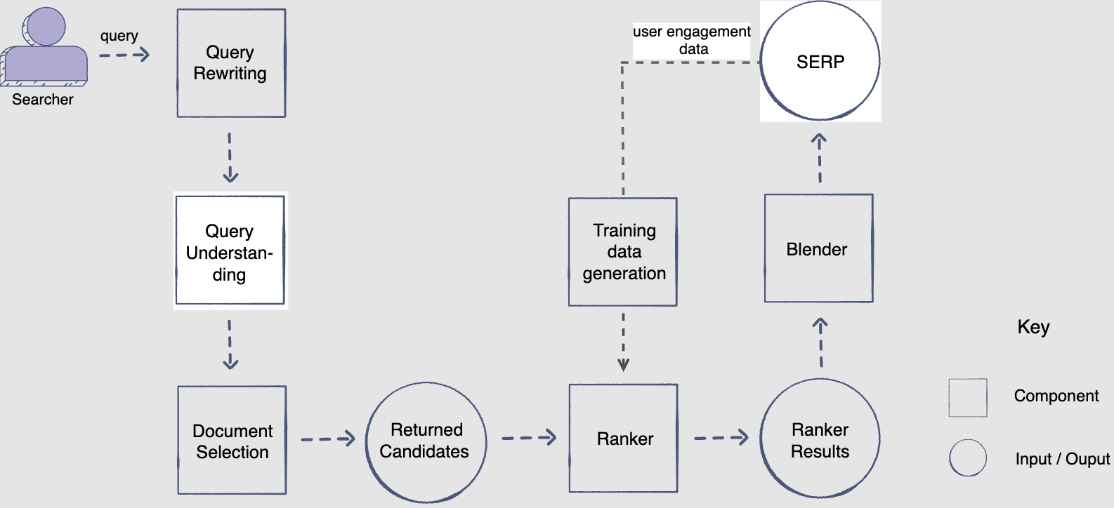
- Let’s briefly look at each component’s role in answering the searcher’s query.
Training Data Generation
Online Experimentation
-
Let’s see how to evaluate the model’s performance through online experimentation.
-
Let’s look at the steps from training the model to deploying it.
Step 1: Training different models
- Earlier, in the training data generation lesson, we discussed a method of splitting the training data for training and validation purposes. After the split, the training data is utilized to train, say, fifteen different models, each with a different combination of hyperparameters, features, and machine learning algorithms. The following figure shows different models are trained to predict user engagement:
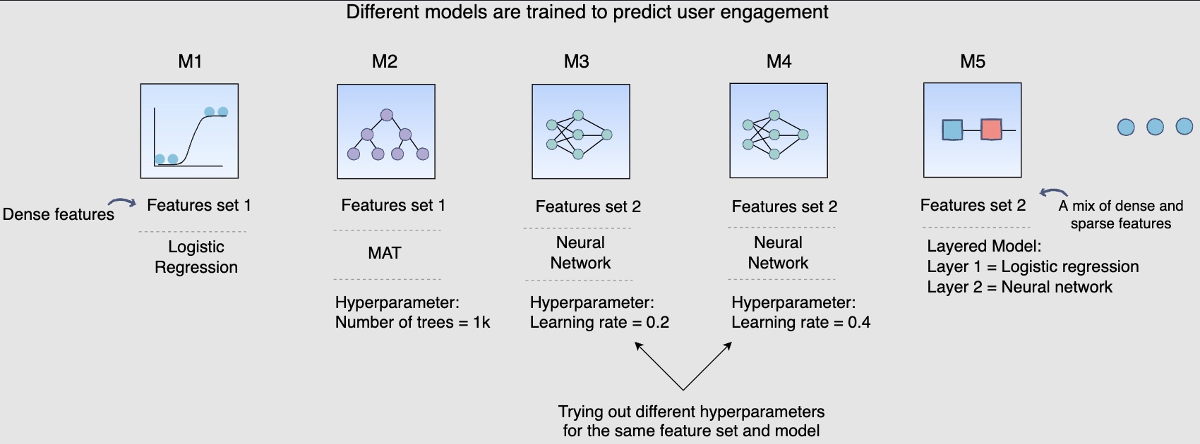
- The above diagram shows different models that you can train for our post engagement prediction problem. Several combinations of feature sets, modeling options, and hyperparameters are tried.
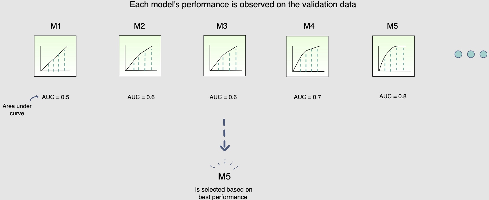
Step 2: Validating models offline
- Once these fifteen models have been trained, you will use the validation data to select the best model offline. The use of unseen validation data will serve as a sanity check for these models. It will allow us to see if these models can generalise well on unseen data. The following figure shows each model’s performance is observed on the validation data
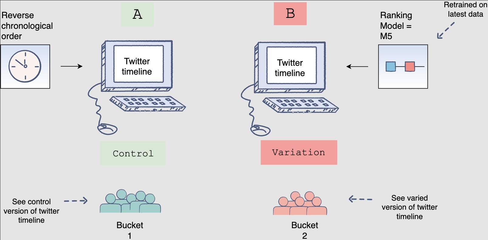
Step 3: Online experimentation
- Now that you have selected the best model offline, you will use A/B testing to compare the performance of this model with the currently deployed model, which displays the feed in reverse chronological order. You will select 1% of the five-hundred million active users, i.e., five million users for the A/B test. Two buckets of these users will be created each having 2.5 million users. Bucket one users will be shown Facebook timelines according to the time-based model; this will be the control group. Bucket two users will be shown the Facebook timeline according to the new ranking model. The following figure shows bucket one users see the control version, whereas Bucket two users see the varied version of the Facebook timeline:
-
However, before you perform this A/B test, you need to retrain the ranking model.
-
Recall that you withheld the most recent partition of the training data to use for validation and testing. This was done to check if the model would be able to predict future engagements on posts given the historical data. However, now that you have performed the validation and testing, you need to retrain the model using the recent partitions of training data so that it captures the most recent phenomena.
Step 4: To deploy or not to deploy
- The results of the A/B tests will help decide whether you should deploy the new ranking model across the platform. The following figure shows engagement aggregates for both buckets of users:
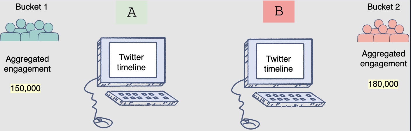
- You can observe that the Facebook feeds generated by the new ranking model had thirty (180k-150k) more engagements.
-
This model is clearly able to outperform the current production, or live state. You should use statistical significance (like p-value) to ensure that the gain is real.
-
Another aspect to consider when deciding to launch the model on production, especially for smaller gains, is the increase in complexity. If the new model increases the complexity of the system significantly without any significant gains, you should not deploy it.
-
To wrap up, if, after an A/B experiment, you see an engagement gain by the model that is statistically significant and worth the complexity it adds to the system, it makes sense to replace the current live system with the new model.
Runtime newsfeed generation
-
Here are issues with running newsfeed generation at runtime:
- We generate the timeline when a user loads their page. This would be quite slow and have a high latency since we have to query multiple tables and perform sorting/merging/ranking on the results.
- Crazy slow for users with a lot of friends/followers as we have to perform sorting/merging/ranking of a huge number of posts.
- For live updates, each status update will result in feed updates for all followers. This could result in high backlogs in our Newsfeed Generation Service.
- For live updates, the server pushing (or notifying about) newer posts to users could lead to very heavy loads, especially for people or pages that have a lot of followers. To improve the efficiency, we can pre-generate the timeline and store it in a memory.
Caching offline generated newsfeeds
-
We can have dedicated servers that are continuously generating users’ newsfeed and storing them in memory for fast processing or in a
UserNewsFeedtable. So, whenever a user requests for the new posts for their feed, we can simply serve it from the pre-generated, stored location. Using this scheme, user’s newsfeed is not compiled on load, but rather on a regular basis and returned to users whenever they request for it. -
Whenever these servers need to generate the feed for a user, they will first query to see what was the last time the feed was generated for that user. Then, new feed data would be generated from that time onwards. We can store this data in a hash table where the “key” would be UserID and “value” would be a STRUCT like this:
Struct {
    LinkedHashMap<FeedItemID, FeedItem> FeedItems;
    DateTime lastGenerated;
}
- We can store
FeedItemIDsin a data structure similar to Linked HashMap or TreeMap, which can allow us to not only jump to any feed item but also iterate through the map easily. Whenever users want to fetch more feed items, they can send the lastFeedItemIDthey currently see in their newsfeed, we can then jump to thatFeedItemIDin our hash-map and return next batch/page of feed items from there.
How many feed items should we store in memory for a user’s feed?
- Initially, we can decide to store 500 feed items per user, but this number can be adjusted later based on the usage pattern.
- For example, if we assume that one page of a user’s feed has 20 posts and most of the users never browse more than ten pages of their feed, we can decide to store only 200 posts per user.
- For any user who wants to see more posts (more than what is stored in memory), we can always query backend servers.
Should we generate (and keep in memory) newsfeeds for all users?
- There will be a lot of users that don’t log-in frequently. Here are a few things we can do to handle this:
- A more straightforward approach could be, to use an LRU based cache that can remove users from memory that haven’t accessed their newsfeed for a long time.
- A smarter solution can be to run ML-based models to predict the login pattern of users to pre-generate their newsfeed, for e.g., at what time of the day a user is active and which days of the week does a user access their newsfeed? etc.
- Let’s now discuss some solutions to our “live updates” problems in the following section.
Practical Tips
- The approach to follow to ensure success is to touch on all aspects of real day-to-day ML. Speak about data, data privacy, the end product, how are the users going to benefit from the system, what is the baseline, success metrics, what modelling choices do we have, can we come with a MVP first and then look at more advanced solutions etc. (say, after identifying bottlenecks and suggesting scaling ideas such as load balancing, caching, replication to improve fault tolerance and data sharding).
Further Reading
- Deep Neural Networks for YouTube Recommendations
- Powered by AI: Instagram’s Explore recommender system
- Google Developers: Recommendation Systems
- Wide & Deep Learning for Recommender Systems
- How TikTok recommends videos #ForYou
- FAISS: A library for efficient similarity search
- Google Developers: Recommendation Systems
- Under the hood: Facebook Marketplace powered by artificial intelligence
- Introducing the Facebook Field Guide to Machine Learning video series
- Github: Minimum Viable Study Plan for Machine Learning Interviews
- Github: The System Design Primer
- Top Facebook System Design Interview Questions Facebook Pirate Interview Round