Distilled • People You May Know (PYMK) RecSys Design
- Problem statement
- Metrics
- Architectural Components
- Candidate Generation
- Training data generation
- Feature Engineering
- Training Data Generation
- Online Experimentation
- Runtime newsfeed generation
- Extended Features
- Practical Tips
- Further Reading
Problem statement
- One of the foundational features of network building on Facebook/LinkedIn is a recommendation system called People You May Know (PYMK). PYMK has been a long-standing part of the Facebook/LinkedIn platform, and is powered by some of our earliest machine learning (ML) algorithms. The goal of PYMK is to help members connect to people who may be relevant additions to their personal networks. There are different reasons why a member might request to be connected with another member on Facebook/LinkedIn, such as staying in touch with past classmates or co-workers, or connecting with long lost friends from childhood.
- This probability that a user would want to connect with another user, \(P(connect)\).
- Snap has a paper on Graph Neural Networks for Friends ranking in a large scale social platform
//: # (- In this paper titled “Friend Story Ranking with Edge-Contextual Local Graph Convolutions,” the authors address the problem of ranking Friend Stories on social platforms, specifically focusing on the task of algorithmic Friend Story Ranking (FSR) with machine learning models. The study explores the use of graph representation learning and proposes an edge-contextual approach called ELR (Edge-Contextual Local Graph Convolutions) to rank Friend Stories based on factors such as local graph structure, edge types, directionality, and rich edge attributes.)
Metrics
- The metrics used in our listing prediction system will help select the best machine-learned models to show relevant PYMK to the user. They should also ensure that these models help the overall improvement of the platform, increase revenue, and provide value for the listing author.
- Like any other optimization problem, there are two types of metrics to measure the effectiveness of our listing prediction system:
- Offline metrics
- Online metrics
Why are both online and offline metrics important? Offline metrics are mainly used to compare the models offline quickly and see which one gives the best result. Online metrics are used to validate the model for an end-to-end system to see how the revenue and engagement rate improve before making the final decision to launch the model.
Offline metrics
- During development, we make extensive use of offline metrics (say, log loss, etc.) to guide iterative improvements to our system.
- The purpose of building an offline measurement set is to be able to evaluate our new models quickly. Offline metrics should be able to tell us whether new models will improve the quality of the recommendations or not.
- Can we build an ideal set of items that will allow us to measure recommendation set quality? One way of doing this could be to look at the items that the user has engaged with and see if your recommendation system gets it right using historical data.
- Once we have the set of items that we can confidently say should be on the user’s recommendation list, we can use the following offline metrics to measure the quality of your recommendation system.
AUC
-
Let’s first go over the area under the receiver operator curve (AUC), which is a commonly used metric for model comparison in binary classification tasks. However, given that the system needs well-calibrated prediction scores, AUC, has the following shortcomings in this listing prediction scenario.
-
AUC does not penalize for “how far off” predicted score is from the actual label. For example, let’s take two positive examples (i.e., with actual label 1) that have the predicted scores of 0.51 and 0.7 at threshold 0.5. These scores will contribute equally to our loss even though one is much closer to our predicted value.
-
AUC is insensitive to well-calibrated probabilities.
-
Log Loss
-
Since, in our case, we need the model’s predicted score to be well-calibrated to use in Auction, we need a calibration-sensitive metric. Log loss should be able to capture this effectively as Log loss (or more precisely cross-entropy loss) is the measure of our predictive error.
-
This metric captures to what degree expected probabilities diverge from class labels. As such, it is an absolute measure of quality, which accounts for generating well-calibrated, probabilistic output.
-
Let’s consider a scenario that differentiates why log loss gives a better output compared to AUC. If we multiply all the predicted scores by a factor of 2 and our average prediction rate is double than the empirical rate, AUC won’t change but log loss will go down.
-
In our case, it’s a binary classification task; a user engages with listing or not. We use a 0 class label for no-engagement (with an listing) and 1 class label for engagement (with an listing). The formula equals:
\[-\frac{1}{N} \sum_{i=1}^{N}\left[y_{i} \log p_{i}+\left(1-y_{i}\right) \log \left(1-p_{i}\right)\right]\]- where:
- \(N\) is the number of observations.
- \(y\) is a binary indicator (0 or 1) of whether the class label is the correct classification for observation.
- \(p\) is the model’s predicted probability that observation is of class (0 or 1).
- where:
Online metrics
- For online systems or experiments, the following are good metrics/KPIs to track:
Connection add rate
- This will measure the ratio of user clicks to PYMK.
Successful session rate
- Time spent scrolling through the list to find connections.
Counter metrics
-
It’s important to track counter metrics to see if the PYMK are negatively impacting the platform.
-
We want the users to keep showing engagement with the platform and PYMK should not hinder that interest. That is why it’s important to measure the impact of PYMK on the overall platform as well as direct negative feedback provided by users. There is a risk that users can leave the platform if PYMK degrade the experience significantly.
-
So, for online PYMK experiments, we should track key platform metrics, e.g., for search engines, is session success going down significantly because of PYMK? Are the average queries per user impacted? Are the number of returning users on the platform impacted? These are a few important metrics to track to see if there is a significant negative impact on the platform.
-
Along with top metrics, it’s important to track direct negative feedback by the user on the listing such as providing following feedback on the listing:
- Hide profile
- Never see this profile
- Report profile as inappropriate
-
These negative sentiments can lead to the perceived notion of the product as negative.
Architectural Components
- Let’s have a look at the high-level architecture of the system. There will be two main actors involved in our listing prediction system - platform users and listing author. Let’s see how they fit in the architecture:
Embedding Based Retrieval in Friend Recommendation
- Friend recommendation systems in online social and professional networks aim to help users find friends and improve user engagement and retention.
- Traditional friend recommendation systems, like Friends-of-Friends (FoF), rely on graph traversal and locality principle but have limitations:
- Limited reach in cold-start scenarios.
- Expensive and infeasible for real-time requests beyond 1 or 2 hops due to latency constraints.
- Inability to capture graph topology and connection strengths effectively, requiring alternative ranking mechanisms for top-K candidates.
- The paper proposes an Embedding Based Retrieval (EBR) system as a solution:
- EBR complements FoF retrieval by retrieving candidates beyond the 2-hop range.
- EBR provides a natural way to rank FoF candidates.
- Online A/B tests demonstrate statistically significant improvements in the number of friendships made when EBR is used as an additional retrieval source.
- Contributions of the paper:
- Deployment of a novel retrieval system in a large-scale friend recommendation system at Snapchat.
- Generation of embeddings for billions of users using Graph Neural Networks.
- Development of EBR infrastructure at Snapchat to support the system at scale.
- The image below (source), depicts the high level architecture of friend recommendation.

- As this paper notes, a users friends are critical for one’s engagement and retention on the app.
Candidate Generation
- In the candidate generation stage, potential friends or connections are identified for a user. One popular approach for candidate generation in PYMK systems is to use Graph Neural Networks (GNNs) such as GraphSAGE or Graph Convolutional Networks (GCNs). GNNs can effectively capture the structural information and patterns in the social graph to generate relevant candidates.
- Graph Representation: The first step is to represent the social graph in a format suitable for GNNs. Each user is considered as a node in the graph, and the connections between users are represented as edges. The graph can include various types of relationships, such as friendships, followings, or mutual connections.
- Graph Convolutional Networks (GCNs): GCNs are one of the early and popular GNN models. They propagate information through the graph using convolutional operations, similar to how convolutional neural networks operate on grid-structured data. GCNs aggregate node features from their immediate neighbors and update node representations.
- GraphSAGE: GraphSAGE (Graph Sample and Aggregator) is another widely used GNN model. It operates by sampling and aggregating information from the neighborhood of each node. GraphSAGE aggregates information from a fixed-size sample of neighboring nodes, allowing it to handle large-scale graphs efficiently.
- Graph Attention Networks (GAT): GATs introduce attention mechanisms to GNNs, enabling nodes to selectively attend to their neighbors during message passing. GATs assign different attention weights to different neighbors based on their relevance to the target node, allowing for more fine-grained information aggregation.
-
Node Embeddings: GNNs operate on node embeddings, which are low-dimensional vector representations of the nodes in the graph. These embeddings capture the features and characteristics of users that are relevant for recommendation. Initial node embeddings can be randomly initialized or obtained from pre-trained models.
-
Message Passing: The core operation in GNNs is message passing, where each node aggregates information from its neighboring nodes. This allows nodes to exchange and update their representations based on the graph structure. Message passing is typically performed iteratively across multiple layers of the GNN.
-
Aggregation and Transformation: During message passing, nodes collect information from their neighbors and aggregate it to update their own embeddings. Common aggregation techniques include summing, averaging, or concatenating the embeddings of neighboring nodes. Additional transformation layers, such as fully connected layers or attention mechanisms, can be applied to refine the aggregated information.
-
Neighborhood Expansion: To generate candidates, the GNN considers the local neighborhood of a user. It expands the neighborhood by iteratively traversing the graph and collecting nodes that are within a certain distance or number of hops from the user. This allows the GNN to capture both direct connections and indirect relationships between users.
-
Candidate Generation: Based on the expanded neighborhood, the GNN generates a set of candidate users who are likely to be potential friends or connections for the target user. These candidates can be ranked or further processed in subsequent stages of the recommendation pipeline.
By leveraging GNNs for candidate generation, the recommendation system can effectively capture the underlying social structure and identify relevant users who are likely to have similar interests, activities, or connections. The generated candidates serve as the initial pool for further retrieval, ranking, and fine ranking stages to provide personalized recommendations to users.
Avoiding inundating people with a lot of friends
- Number of mutual friends is a critical signal. However, a user may game the system by sending friend requests to a bunch of your connections or might be a person who receives a large number of friend requests, e.g., , an influencer in an industry, a high-profile senior executive, or a recruiter from a big company. At a high level, having a disproportionate number of friend requests may appear to simply run counter to our stated goal of closing the network gap. However, it can also lead to the member’s network becoming overrun with feed updates and notifications that may seem random or from members who are only tangentially relevant to their own career. A member inundated with invites may also simply miss relevant networking opportunities. This negative experience showed up both in the data about how these members were using PYMK and in the form of direct user feedback.
- In order to address this problem, we added a re-ranker on top of the P(connect) score by discounting/decaying the score of recipients with an excess number of invitations. In other words, as a recipient receives more and more invitations, the original score needs to be higher and higher in order for them to show up in PYMK results.
- To understand how the system works, let us take a simple example. In the above figure, we have a ranked list of recommendations and the number on the top right shows the number of invitations already received by the member. Candidate A is ranked in the top position before we decay the score. To re-rank members, we compute newScore = score * df , where score is pConnect and df is the decay factor in [0,1]. Suppose we want to deprioritize recipients who have received >10 invitations in the past week. After decay, A’s new score becomes smaller, hence A becomes ranked below B, C, and D. In production, we use a piecewise linear function to compute the decay factor given the number of invitations received.
GNN approach = Friends-of-Friends (FoF)
- Data Collection: Gather user profile information, social connections, interactions, and other relevant data.
- Feature Extraction: Extract features from the collected data to represent users and their relationships. This can include attributes like mutual friends, shared interests, education, work history, location, etc.
- Graph Construction: Build a social graph representing the connections between users based on their relationships and interactions.
- Neighborhood Expansion: Expand the immediate connections of a user by traversing the graph to include friends-of-friends or connections up to a certain depth. This helps in generating a pool of potential candidates.
- Can leverage GCN or GraphSage for embeddings:
- GraphSAGE is particularly suitable for large-scale graphs as it employs neighborhood sampling to aggregate information from a subset of neighbors. It allows the algorithm to scale well and handle graphs with millions or even billions of nodes.
- GCN, on the other hand, is a more straightforward and interpretable GNN model. It propagates information through graph convolutions, considering the direct connections between nodes. This can be useful for capturing the local connectivity patterns in the graph.
Bipartite graph
- Two types of nodes only interact with each other (user and items)
Retrieval = Coarse
- Contrastive ranking against randomly sampled negative
- This indicates a ranking methodology that utilizes contrastive learning. Contrastive learning is a technique used in machine learning where positive and negative examples are compared to learn useful representations. In this case, during the ranking process, the system compares positive (relevant) examples against randomly sampled negative (non-relevant) examples. The goal is to learn a ranking model that can differentiate between relevant and non-relevant items effectively.
- Can be done via ANN
-
- ANN model takes these embeddings and performs additional computations or transformations to generate recommendation candidates. The ANN can incorporate various features, including node embeddings, user preferences, item attributes, or contextual information, depending on the specific recommendation task.
Bloom Filter
- Membership Test: To check if an item is a member of the set, the item is passed through the same hash functions, and the corresponding bits in the bit array are checked. If any of the bits are 0, the item is definitely not present in the set. If all the bits are 1, the item is considered a potential member (a false positive).
- Bloom filters are often used in recommendation systems to speed up the retrieval of potential candidates by pre-filtering the data. They help reduce the number of unnecessary expensive lookups or computations by quickly eliminating candidates that are highly unlikely to be relevant based on simple hash-based checks.
- A Bloom filter is a probabilistic data structure used to quickly check whether an element is a member of a set or not.
Ranking
- Ranking: After computing the similarities, the candidates are ranked based on their similarity scores. The most similar candidates are given higher ranks, indicating their potential relevance to the target user.
- The ranking process is crucial as it determines the final order in which the candidates are presented to the user.
- Rank on P(click)
Challenges
- Structural sparsity: Very few friends
- Interaction sparsity: very small fraction of users actively form new friendships
Sparsity:
- Graph Augmentation: Add Auxiliary Nodes: Introduce additional nodes to the graph that represent common interests, communities, or other relevant attributes. Connect these auxiliary nodes to the existing user nodes to provide additional information and potentially bridge gaps in the graph structure. Connect Seed Nodes: Create connections between seed nodes (users) who have few friends. This can help create a bridge between users with limited connections and facilitate recommendations based on commonalities.
- Neighbor Sampling: Selective Sampling: Instead of considering the entire neighborhood of a user, perform selective sampling by choosing a subset of neighbors based on certain criteria (e.g., highest degree nodes, nodes with similar attributes). This approach focuses on the most informative neighbors, enabling better recommendations even in sparse scenarios. Incorporate Unconnected Nodes: During neighbor sampling, include unconnected nodes as potential neighbors. This allows for the exploration of new connections and potential friendships.
- Content Information: User Attributes: Incorporate user attributes or features, such as age, location, interests, or demographics, into the node representations. These attributes can provide additional context for generating friend recommendations and compensate for sparsity in the graph structure. Content-Based Similarity: Calculate similarity between users based on their attribute vectors. This similarity measure can be combined with the learned node embeddings to enhance the friend recommendation process.
Multi-faceted friend Ranking
- Multi modal user features

- these features are extracted by routine jobs
-
Listing Ranking/Scoring/Prediction
- After we get the retrieval result, we perform a final ranking using a Sparse Neural Network model with online training. Because the ranking stage model uses more data and more real-time signals (such as the counters of the real-time events that happened on each of the products), it is more accurate — but it’s also computationally heavier, so we do not use it as the model at the retrieval stage; we use it once we’ve already narrowed down the list of all possible items.
- Using more similarity searches and Lumos, Facebook has recently launched another feature to recommend products based on listing images. So if a buyer shows interest in a specific lamp that is no longer available, the system can search the database for similar lamps and promptly recommend several that may be of interest to the buyer.
Training data generation
- We need to record the action taken on an listing. This component takes user action on the PYMK (displayed after the auction) and generates positive and negative training examples for the listing prediction component.
Funnel model approach
-
For a large scale PYMK prediction system, it’s important to quickly select an listing for a user based on either the search query and/or user interests. The scale can be large both in terms of the number of PYMK in the system and the number of users on the platform. So, it’s important to design the system in a way that it can scale well and be extremely performance efficient without compromising on PYMK quality.
-
To achieve the above objective, it would make sense to use a funnel approach, we gradually move from a large set of PYMK to a more precise set for the next step in the funnel.
-
Funnel approach: get relevant PYMK for a user:

-
As we go down the funnel (as shown in the diagram), the complexity of the models becomes higher and the set of PYMK that they run on becomes smaller. It’s also important to note that the initial layers are mostly responsible for PYMK selection. On the other hand, PYMK prediction is responsible for predicting a well-calibrated engagement and quality score for PYMK. This predicted score is going to be utilized in the auction as well.
-
Let’s go over an example to see how these components will interact for the search scenario.
- A thirty-year old male user issues a query “machine learning”.
- The PYMK selection component selects all the PYMK that match the targeting criteria ( user demographics and query) and uses a simple model to predict the listing’s relevance score.
- The PYMK selection component ranks the PYMK according to \(r=\text { bid } * \text { relevance }\) and sends the top PYMK to our PYMK prediction system.
- The PYMK prediction component will go over the selected PYMK and uses a highly optimized ML model to predict a precise calibrated score.
- The PYMK auction component then runs the auction algorithm based on the bid and predicted PYMK score to select the top most relevant PYMK that are shown to the user.
-
We will zoom into the different segments of this diagram as we explore each segment in the upcoming lessons.
Feature Engineering
-
Features are the backbone of any learning system. Let’s think about the main actors or dimensions that will play a key role in our feature engineering process.
- User
- Connection
- Context
-
Now it’s time to generate features based on these actors. The features would fall into the following categories:
- User specific features
- Connection specific features
- User-connection cross features
User/Connection specific features
age: This feature records the age of the user. It allows the model to learn the kind of listing that is appropriate according to different age groups.region: This feature records the country of the user. Users from different geographical regions have different content preferences. This feature can help the model learn regional preferences and tune the recommendations accordingly.language: This feature records the language of the user.friends_list: The user’s friend list to calculate mutual friends.education_embedding: The user’s educational institutions in embedding form.education_timespan: The user’s education timespan.current_work_embedding: The user’s current workplace in embedding form.prior_work_embedding: The user’s prior workplaces in embedding form.prior_work_timespan: The user’s prior workplace timespan.stay_places: The places of the user’s stay.stay_timespan: The timespans of the user’s stay.interests: The user’s interests.pages_liked_topics_embedding: The topics of the user’s liked pages.groups_joined_topics_embedding: The topics of the user’s joined groups.
Training Data Generation
- The performance of the user engagement prediction model will depend drastically on the quality and quantity of training data. So let’s see how the training data for our model can be generated.
Training data generation through online user engagement
-
When we show an listing to the user, they can engage with it or ignore it. Positive examples result from users engaging with PYMK, e.g., clicking or listingding an item to their cart. Negative examples result from users ignoring the PYMK or providing negative feedback on the listing.
-
Suppose the listing author specifies “click” to be counted as a positive action on the listing. In this scenario, a user-click on an listing is considered as a positive training example, and a user ignoring the listing is considered as a negative example.
-
Click counts as positive example:
- Suppose the listing refers to an online shopping platform and the listing author specifies the action “listingd to cart” to be counted as positive user engagement. Here, if the user clicks to view the listing and does not listingd items to the cart, it is counted as a negative training example.
- “listingd to cart” counts as a positive training example:
Balancing positive and negative training examples
-
Users’ engagement with an listing can be fairly low based on the platform e.g. in case of a feed system where people generally browse content and engage with minimal content, it can be as low as 2-3%.
-
How would this percentage affect the ratio of positive and negative examples on a larger scale?
-
Let’s look at an extreme example by assuming that one-hundred million PYMK are viewed collectively by the users in a day with a 2% engagement rate. This will result in roughly two million positive examples (where people engage with the listing) and 98 million negative examples (where people ignore the listing).
-
In order to balance the ratio of positive and negative training samples, we can randomly down sample the negative examples so that we have a similar number of positive and negative examples.
Model recalibration
- Negative downsampling can accelerate training while enabling us to learn from both positive and negative examples. However, our predicted model output will now be in the downsampling space. For instance, consider that if our engagement rate is 5% and we select only 10% negative samples, our average predicted engagement rate will be near 50%.
-
Auction uses this predicted rate to determine order and pricing; therefore it’s critical that we recalibrate our score before sending them to auction. The recalibration can be done using:
\[q=\frac{p}{p+(1-p) / w}\] - where,
- \(q\) is the re-calibrated prediction score,
- \(p\) is the prediction in downsampling space, and
- \(w\) is the negative downsampling rate.
Train test split
-
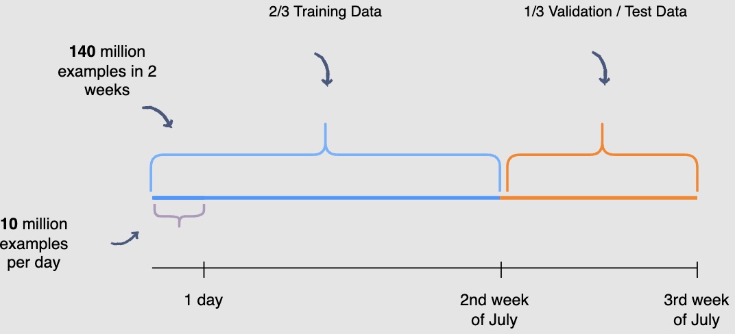
You need to be mindful of the fact that the user engagement patterns may differ throughout the week. Hence, you will use a week’s engagement to capture all the patterns during training data generation. At this rate, you would end up with around seventy million rows of training data.
-
You may randomly select \(\frac{2}{3}^{rd}\) or 66.6% , of the seventy million training data rows that you have generated and utilize them for training purposes. The rest of the \(\frac{1}{3}^{rd}\) or 33.3%, can be used for validation and testing of the model. However, this random splitting defeats the purpose of training the model on an entire week’s data. Also, the data has a time dimension, i.e., we know the engagement on previous posts, and we want to predict the engagement on future posts ahelisting of time. Therefore, you will train the model on data from one time interval and validate it on the data with the succeeding time interval. This will give a more accurate picture of how the model will perform in a real scenario.
We are building models with the intent to forecast the future.
- In the following illustration, we are training the model using data generated from the first and second week of July and data generated in the thirdweek of July for validation and testing purposes. THe following diagram indicates the splitting data procedure for training, validation, and testing:
- Possible pitfalls seen after deployment where the model is not offering predictions with great accuracy (but performed well on the validation/test splits): Question the data. Garbage in - Garbage out. The model is only as good as the data it was trained on. Data drifts where the real-world data follows a different distribution that the model was trained on are fairly common.
- When was the data acquired? The more recent the data, better the performance of the model.
- Does the data show seasonality? i.e., we need to be mindful of the fact that the user engagement patterns may differ throughout the week. For e.g., don’t use data from weekdays to predict for the weekends.
- Was the data split randomly? Random splitting defeats the purpose since the data has a time dimension, i.e., we know the engagement on previous posts, and we want to predict the engagement on future posts ahelisting of time. Therefore, you will train the model on data from one time interval and validate it on the data with the succeeding time interval.
Online Experimentation
-
Let’s see how to evaluate the model’s performance through online experimentation.
-
Let’s look at the steps from training the model to deploying it.
Step 1: Training different models
- Earlier, in the training data generation lesson, we discussed a method of splitting the training data for training and validation purposes. After the split, the training data is utilized to train, say, fifteen different models, each with a different combination of hyperparameters, features, and machine learning algorithms. The following figure shows different models are trained to predict user engagement:

- The above diagram shows different models that you can train for our post engagement prediction problem. Several combinations of feature sets, modeling options, and hyperparameters are tried.
Step 2: Validating models offline
- Once these fifteen models have been trained, you will use the validation data to select the best model offline. The use of unseen validation data will serve as a sanity check for these models. It will allow us to see if these models can generalise well on unseen data. The following figure shows each model’s performance is observed on the validation data

Step 3: Online experimentation
- Now that you have selected the best model offline, you will use A/B testing to compare the performance of this model with the currently deployed model, which displays the feed in reverse chronological order. You will select 1% of the five-hundred million active users, i.e., five million users for the A/B test. Two buckets of these users will be created each having 2.5 million users. Bucket one users will be shown Facebook timelines according to the time-based model; this will be the control group. Bucket two users will be shown the Facebook timeline according to the new ranking model. The following figure shows bucket one users see the control version, whereas Bucket two users see the varied version of the Facebook timeline:

-
However, before you perform this A/B test, you need to retrain the ranking model.
-
Recall that you withheld the most recent partition of the training data to use for validation and testing. This was done to check if the model would be able to predict future engagements on posts given the historical data. However, now that you have performed the validation and testing, you need to retrain the model using the recent partitions of training data so that it captures the most recent phenomena.
Step 4: To deploy or not to deploy
- The results of the A/B tests will help decide whether you should deploy the new ranking model across the platform. The following figure shows engagement aggregates for both buckets of users:

- You can observe that the Facebook feeds generated by the new ranking model hlisting thirty (180k-150k) more engagements.
-
This model is clearly able to outperform the current production, or live state. You should use statistical significance (like p-value) to ensure that the gain is real.
-
Another aspect to consider when deciding to launch the model on production, especially for smaller gains, is the increase in complexity. If the new model increases the complexity of the system significantly without any significant gains, you should not deploy it.
-
To wrap up, if, after an A/B experiment, you see an engagement gain by the model that is statistically significant and worth the complexity it listingds to the system, it makes sense to replace the current live system with the new model.
Runtime newsfeed generation
-
Here are issues with running newsfeed generation at runtime:
- We generate the timeline when a user loPYMK their page. This would be quite slow and have a high latency since we have to query multiple tables and perform sorting/merging/ranking on the results.
- Crazy slow for users with a lot of friends/followers as we have to perform sorting/merging/ranking of a huge number of posts.
- For live updates, each status update will result in feed updates for all followers. This could result in high backlogs in our Newsfeed Generation Service.
- For live updates, the server pushing (or notifying about) newer posts to users could lelisting to very heavy loPYMK, especially for people or pages that have a lot of followers. To improve the efficiency, we can pre-generate the timeline and store it in a memory.
Caching offline generated newsfeeds
-
We can have dedicated servers that are continuously generating users’ newsfeed and storing them in memory for fast processing or in a
UserNewsFeedtable. So, whenever a user requests for the new posts for their feed, we can simply serve it from the pre-generated, stored location. Using this scheme, user’s newsfeed is not compiled on lolisting, but rather on a regular basis and returned to users whenever they request for it. -
Whenever these servers need to generate the feed for a user, they will first query to see what was the last time the feed was generated for that user. Then, new feed data would be generated from that time onwards. We can store this data in a hash table where the “key” would be UserID and “value” would be a STRUCT like this:
Struct {
    LinkedHashMap<FeedItemID, FeedItem> FeedItems;
    DateTime lastGenerated;
}
- We can store
FeedItemIDsin a data structure similar to Linked HashMap or TreeMap, which can allow us to not only jump to any feed item but also iterate through the map easily. Whenever users want to fetch more feed items, they can send the lastFeedItemIDthey currently see in their newsfeed, we can then jump to thatFeedItemIDin our hash-map and return next batch/page of feed items from there.
How many feed items should we store in memory for a user’s feed?
- Initially, we can decide to store 500 feed items per user, but this number can be listingjusted later based on the usage pattern.
- For example, if we assume that one page of a user’s feed has 20 posts and most of the users never browse more than ten pages of their feed, we can decide to store only 200 posts per user.
- For any user who wants to see more posts (more than what is stored in memory), we can always query backend servers.
Should we generate (and keep in memory) newsfeeds for all users?
- There will be a lot of users that don’t log-in frequently. Here are a few things we can do to handle this:
- A more straightforward approach could be, to use an LRU based cache that can remove users from memory that haven’t accessed their newsfeed for a long time.
- A smarter solution can be to run ML-based models to predict the login pattern of users to pre-generate their newsfeed, for e.g., at what time of the day a user is active and which days of the week does a user access their newsfeed? etc.
- Let’s now discuss some solutions to our “live updates” problems in the following section.
Extended Features
Enriching buyer and seller interactions by suggesting message responses
- Messenger allows buyers and sellers to communicate about a product directly. When chatting in Messenger, M, an automated assistant powered by AI, makes suggestions to help people communicate and get things done. For example, in a 1:1 conversation, when a seller is asked a question such as “Is the bicycle still available?” M can suggest replies like “Yes,” “No,” or “I think so.”
Missed an item? Let Facebook find you similar ones
- If the answer is no, the product is no longer available, then M may prompt the buyer with a suggestion to “Find more like this on Marketplace” with a link to a page of items similar to the one the buyer was asking about. This list is compiled using our similarity search functionality.
Message language detection and translation
-
If M detects that a person received a message in a language that is different from his or her default language, it will offer to translate this message. Messages are translated using our neural machine translation platform, the same technology that translates posts and comments on Facebook and Instagram.
-
All these suggestions are automatically generated by an AI system that was trained via machine learning to recognize intent. We use different neural net models to determine the intent and whether to show a suggestion. We also use entity extractors like Duckling to identify things like dates, times, and locations. For some suggestions, we use additional neural net models to rank different suggestions to ensure the most relevant options are surfaced (like translation, stickers, or replies). M also learns and becomes more personalized over time, so if you interact with one suggestion more regularity, M might surface it more. If you use another less (or not at all), M will adapt accordingly. This entire process is automated and powered by artificial intelligence.
Practical Tips
- The approach to follow to ensure success is to touch on all aspects of real day-to-day ML. Speak about data, data privacy, the end product, how are the users going to benefit from the system, what is the baseline, success metrics, what modelling choices do we have, can we come with a MVP first and then look at more listingvanced solutions etc. (say, after identifying bottlenecks and suggesting scaling ideas such as lolisting balancing, caching, replication to improve fault tolerance and data sharding).
Further Reading
- Deep Neural Networks for YouTube Recommendations
- Powered by AI: Instagram’s Explore recommender system
- Google Developers: Recommendation Systems
- Wide & Deep Learning for Recommender Systems
- How TikTok recommends videos #ForYou
- Design the “People You May Know” feature on LinkedIn or Facebook
- How friend suggestions or 2nd degree related (linkedin) algorithm works
- How does LinkedIn’s People You May Know work?
- Building a heterogeneous social network recommendation system
- Optimizing People You May Know (PYMK) for equity in network creation
- FAISS: A library for efficient similarity search
- Google Developers: Recommendation Systems
- Under the hood: Facebook Marketplace powered by artificial intelligence