Distilled • Newsfeed RecSys Design
- Problem statement
- Visualizing the problem
- Requirements
- Scale Estimation and Performance/Capacity Requirements
- Metrics
- Architectural Components
- Post Retrieval/Selection
- Feature Engineering
- Training Data Generation
- Ranking: Modeling
- Diversity/Re-ranking
- Online Experimentation
- Runtime newsfeed generation
- Model Selection
- Evaluation
- Calculation & estimation#
- High-level design
- Scale the design
- Practical Tips
- Further Reading
Problem statement
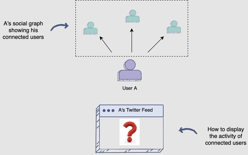
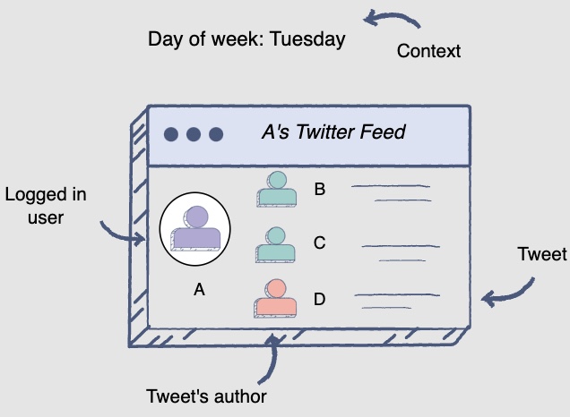
- The interviewer has asked you to design the ML bits of the Facebook Newsfeed system that will show the most relevant posts for a user based on their social graph. The following diagram shows how to display the most relevant content for user A’s Facebook feed:
-
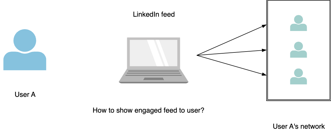
Design a personalized LinkedIn feed to maximize long-term user engagement. One way to measure engagement is user frequency, i.e, measure the number of engagements per user, but it’s very difficult in practice. Another way is to measure the click probability or Click Through Rate (CTR).
-
On the LinkedIn feed, there are five major activity types:
- Connections (A connects with B)
- Informational
- Profile
- Opinion
- Site-specific
- Intuitively different activities have very different CTR. This is important when we decide to build models and generate training data.
Visualizing the problem
-
User A is connected to other people/businesses on the Facebook platform. They are interested in knowing the activity of their connections through their feed.
-
In the past, a rather simplistic approach has been followed for this purpose. All the posts generated by their followees since user A’s last visit were displayed in reverse chronological order.
-
However, this reverse-chronological order feed display often resulted in user A missing out on some posts that they would have otherwise found very engaging. Let’s see how this happens.
-
Facebook experiences a large number of daily active users, and as a result, the amount of data generated on Facebook is torrential. Therefore, a potentially engaging post may have gotten pushed further down in the feed because a lot of other posts were posted after it.
-
Hence, to provide a more engaging user experience, it is crucial to rank the most relevant posts above the other ones based on user interests and social connections. Transition from time-based ordering to relevance-based ordering of Facebook feed:
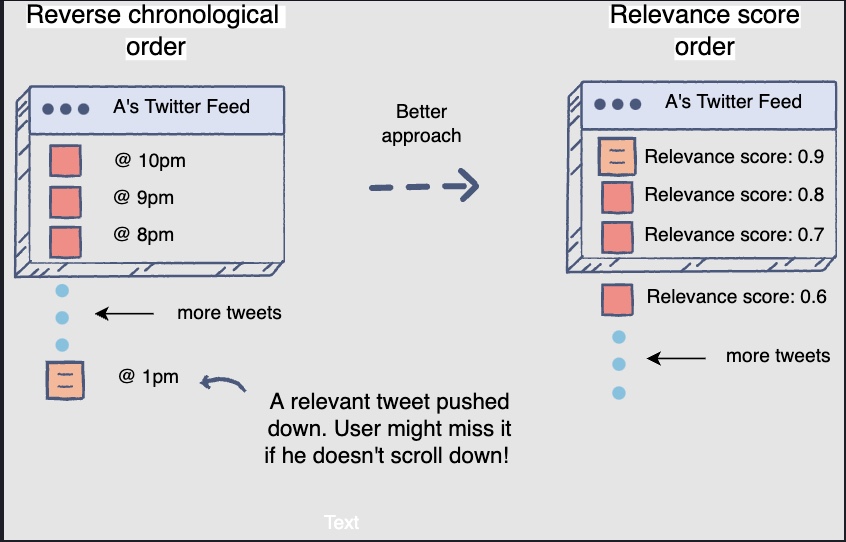
- The feed can be improved by displaying activity based on its relevance for the logged-in user. Therefore, the feed order is now based on relevance ranking.
Requirements
- Training
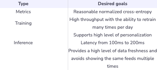
- We need to handle large volumes of data during training. Ideally, the models are trained in distributed settings. In social network settings, it’s common to have online data distribution shift from offline training data distribution. One way to address this issue is to retrain the models (incrementally) multiple times per day.
- Personalization: Support is needed for a high level of personalization since different users have different tastes and styles for consuming their feed.
- Data freshness: Avoid showing repetitive feed on the user’s home feed.
- Inference
- Scalability: The volume of users’ activities are large and the LinkedIn system needs to handle 300 million users.
- Latency: When a user goes to LinkedIn, there are multiple pipelines and services that will pull data from multiple sources before feeding activities into the ranking model. All of these steps need to be done within 200ms. As a result, the Feed Ranking needs to return within 50ms.
- Data freshness: Feed Ranking needs to be fully aware of whether or not a user has already seen any particular activity. Otherwise, seeing repetitive activity will compromise the user experience. Therefore, data pipelines need to run really fast.
Scale Estimation and Performance/Capacity Requirements
- Now that you know the problem at hand, let’s define the scope of the problem:
- Daily Active Users (DAUs): 2B (by current Facebook estimates, as of April 2022)
- Newsfeed requests: Each user fetching their timeline an average of ten times a day, leading to 10B newsfeed requests per day or approximately 116K requests per second.
- Each user has 300 friends and follows 200 pages.
- Finally, let’s set up the machine learning problem: “Given a list of posts, train an ML model that predicts the probability of engagement of posts and orders them based on that score”
Metrics
Offline metrics
- During development, we make extensive use of offline metrics (say, log loss, etc.) to guide iterative improvements to our system.
- The purpose of building an offline measurement set is to be able to evaluate our new models quickly. Offline metrics should be able to tell us whether new models will improve the quality of the recommendations or not.
- Can we build an ideal set of items that will allow us to measure recommendation set quality? One way of doing this could be to look at the items that the user has engaged with and see if your recommendation system gets it right using historical data.
- Once we have the set of items that we can confidently say should be on the user’s recommendation list, we can use the following offline metrics to measure the quality of your recommendation system.
- The Click Through Rate (CTR) for one specific feed is the number of clicks that feed receives, divided by the number of times the feed is shown.
- Maximizing CTR can be formalized as training a supervised binary classification model. For offline metrics, we normalize cross-entropy and AUC.
- Normalizing cross-entropy (NCE) helps the model be less sensitive to background CTR.
Online metrics: user engagement/actions
- For non-stationary data, offline metrics are not usually a good indicator of performance. Online metrics need to reflect the level of engagement from users once the model has deployed, i.e., Conversion rate (ratio of clicks with number of feeds).
- The feed-ranking system aims to maximize user engagement. So, let’s start by looking at all the user actions on a Facebook feed.
- For the final determination of the effectiveness of an algorithm or model, we rely on A/B testing via live experiments. In a live experiment, we can measure subtle changes in click-through rate (CTR), watch time, and many other metrics that measure user engagement. This is important because live A/B results do not always correlate with offline experiments.
- The following are some of the actions that the user will perform on their post, categorized as positive and negative actions.
- Positive user actions:
- Time spent viewing the post (a.k.a. dwell time).
- Liking a post.
- Commenting on a post.
- Sharing a post.
- Saving a post.
- Click-Through Rate (CTR) for links on the newsfeed.
- Negative user actions:
- Hiding a post.
- Reporting posts as inappropriate.
- Positive user actions:
- Now, you need to look at these different forms of engagements on the feed to see if your feed ranking system did a good job.
All of the metrics we are going to discuss can be used to determine the user engagement of the feed generated by our feed ranking system.
User engagement metrics
- The following illustration shows how feed engagement data generates useful statistics for gauging user engagement.
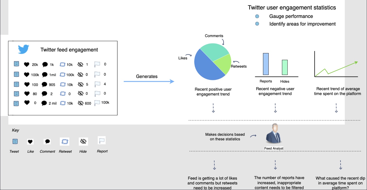
- The above illustration shows different positive and negative engagements on a Facebook feed. Let’s see which of these engagements would be a good one to target as your overall system metric to optimize for.
Selecting feed optimization metric
-
An important thing to understand in selecting a topline is that it’s scientific as well as a business-driven decision.
-
The business might want to focus on one aspect of user engagement. For instance, Facebook can decide that the Facebook community needs to engage more actively in a dialogue. So, the topline metric would be to focus more on the number of comments on the posts. If the average number of comments per user increases over time, it means that the feed system is helping the business objective.
-
Similarly, Facebook might want to shift its focus to overall engagement. Then their objective will be to increase average overall engagement, i.e., comments, likes, and shares. Alternatively, the business may require to optimize for the time spent on the application. In this case, time spent on Facebook will be the feed system metric.
Negative engagement or counter metric
- For any system, it’s super important to think about counter metrics along with the key, topline ones. In a feed system, users may perform multiple negative actions such as reporting a post as inappropriate, block a user, hide a post, etc. Keeping track of these negative actions and having a metric such as average negative action per user is also crucial to measure and track.
Weighted engagement
-
More often than not, all engagement actions are equally important. However, some might become more important at a particular point in time, based on changing business objectives. For example, to have an engaged audience, the number of comments might be more critical rather than just likes. As a result, we might want to have different weights for each action and then track the overall engagement progress based on that weighted sum. So, the metric would become a weighted combination of these user actions. The weighted combination metric can be thought of as a value model. It will summarize multiple impacts (of different forms of user engagements) into a single score. Let’s see how this works.
-
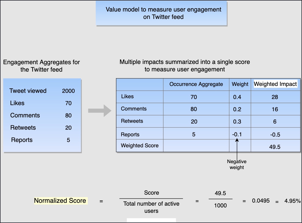
In the following illustration, we are going to use the weighted combination metric to measure/score user engagement. Each user action will be assigned a weight according to the impact it should have towards the final score.
These weights are assigned, keeping in mind the respective importance of different forms of engagement towards the business objectives.
-
Using the weighted metric to measure the performance of the feed, i.e., it’s user engagement The user engagements are aggregated across all users’ feeds over a specific period of time. In the above diagram, two-thousand posts were viewed in a day on Facebook. There were a total of seventy likes, eighty comments, twenty shares, and five reports. The weighted impact of each of these user engagements is calculated by multiplying their occurrence aggregate by their weights. In this instance, Facebook is focusing on increasing “likes” the most. Therefore, “likes” have the highest weight. Note that the negative user action, i.e., “report”, has a negative weight to cast its negative impact on the score.
-
The weighted impacts are then summed up to determine the score. The final step is to normalize the score with the total number of active users. This way, you obtain the engagement per active user, making the score comparable. To explain the importance of normalization, consider the following scenario.
-
The score calculated above is referred to as score A, in which we considered one-thousand active users. We now calculate the score over a different period where there are only five-hundred active users, referred to as score B. Assume that score B comes out to be less than score A. Now, score A and score B are not comparable. The reason is that the decrease in score B may just be the effect of less active users (i.e., five-hundred active users instead of one-thousand active users).
-
When it comes to interpretation, a higher score equates to higher user engagement.
-
The weights can be tweaked to find the desired balance of activity on the platform. For example, if we want to increase the focus on commenting, we can increase its weight. This would put us on the right track, i.e., we would be showing posts that get more comments. This will lead to an increase in the overall score, indicating good performance.
Architectural Components
- Have a look at the architectural components of the feed ranking system.
Architecture
- Let’s have a look at the architectural components that are integral in creating our Facebook feed system.
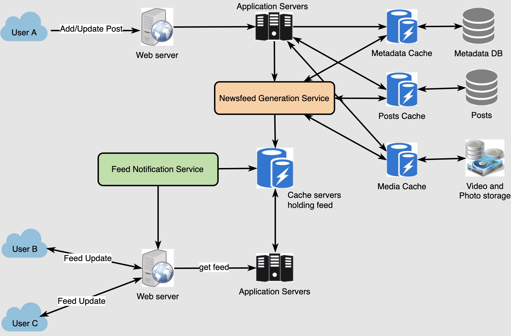
- Let’s briefly look at each component here. Further explanation will be provided in the following lessons.
Post selection
- This component performs the first step in generating a user’s feed, i.e., it fetches a pool of posts from the user’s network (the followees), since their last login. This pool of posts is then forwarded to the ranker component.
Training data generation
- Each user engagement action on the Facebook feed will generate positive and negative training examples for the user engagement prediction models.
Post Retrieval/Selection
- Let’s see how the post selection component fetches posts to display on a user’s Facebook feed.
New posts
-
Consider the following scenario to see how post selection occurs.
-
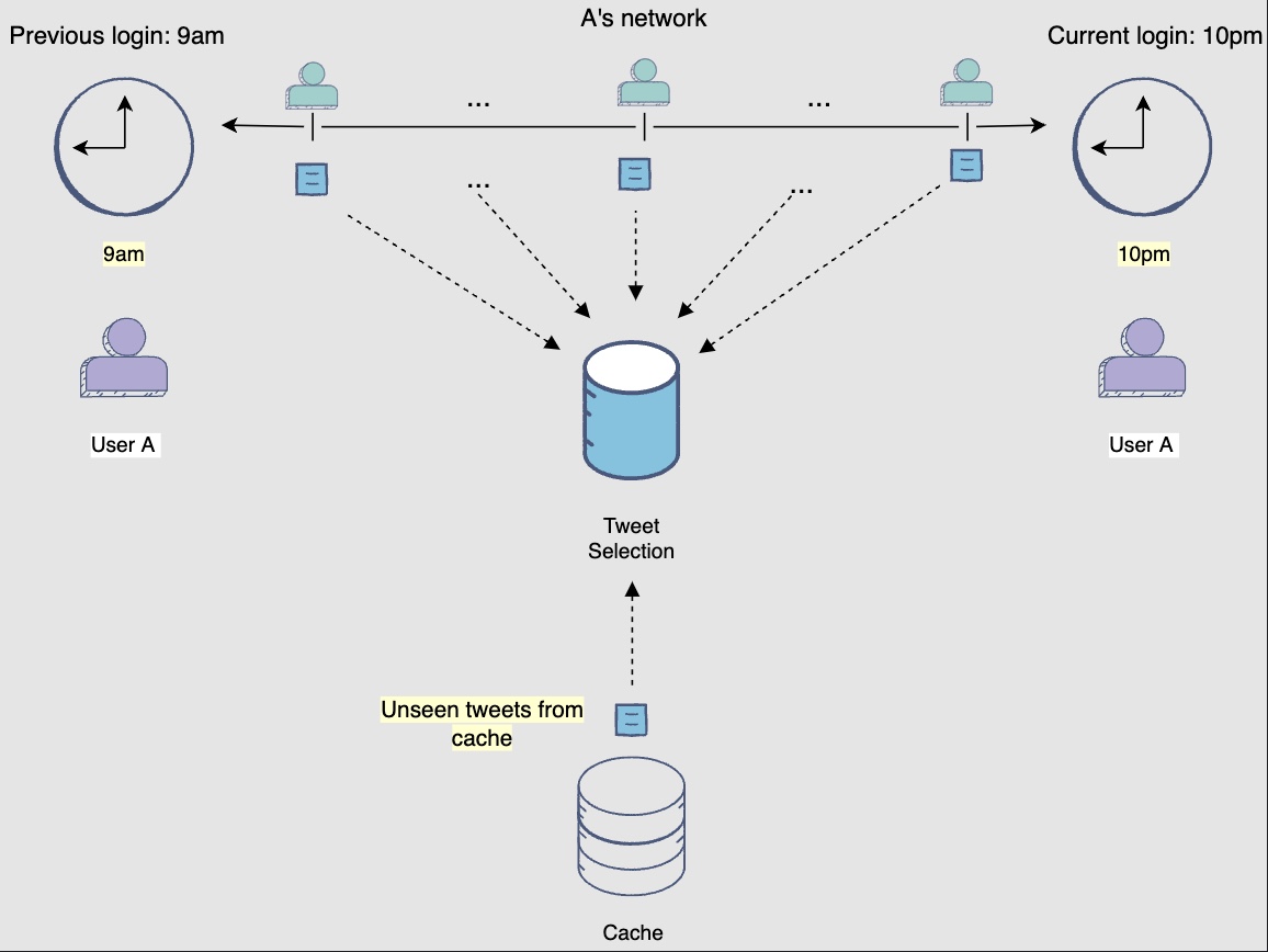
User A logs in to Facebook at 9 am to view their Facebook feed. Now, the post selection component has to fetch posts for display. It fetches the five-hundred newly generated posts by A’s network since the last login at 3 pm yesterday. This following diagram illustrates selection of new posts generated by A’s network between 3pm to 9am:
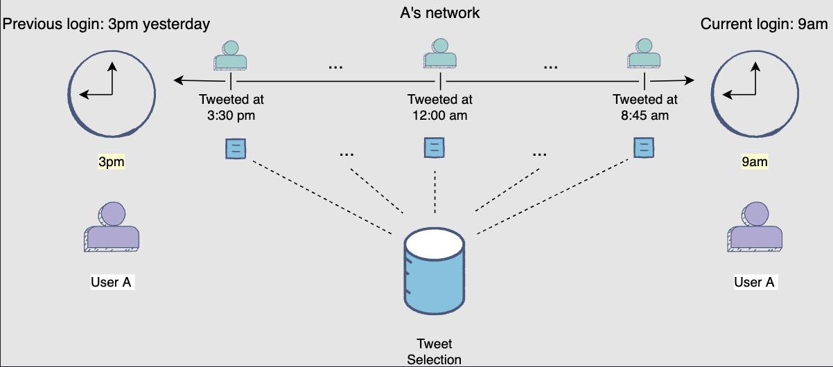
A not-so-new post! Consider a post that user A has viewed previously. However, by the time the user logs in again, this post has received a much bigger engagement and/or A’s network has interacted with it. In this case, it once again becomes relevant to the user due to its recent engagements. Now, even though this post isn’t new, the post selection component will select it again so that the user can view the recent engagements on this post.
New posts + Old unseen posts
-
Picking up where we left off, let’s see how this component may select a mix of new and old unseen posts.
-
The new posts fetched in the previous step are ranked and displayed on user A’s feed. They only view the first two-hundred posts and log out. The ranked results are also stored in a cache.
-
Now, user A logs in again at 10 pm. According to the last scheme, the post selection component should select all the new posts generated between 9 am and 10 pm. However, this may not be the best idea!
-
For 9am’s feed, the component previously selected a post made at 8:45 am. Since this post was recently posted, it did not have much user engagement at that time. Therefore, it was ranked at the \(450^{th}\) position in the feed. Now, remember that A logged out after only viewing the first two-hundred posts and this post remained unread. Since the user’s last visit, this unread post gathered a lot of attention in the form of reshares, likes, and comments. The post selection component should now reconsider this post’s selection. This time it would be ranked higher, and A will probably view it.
-
Keeping the above rationale in mind, the post selection component now fetches a mix of newly generated posts along with a portion of old unseen posts (especially the popular ones) from the cache.
- You may encounter the following edge case during post selection.
Edge case: User returning after a while
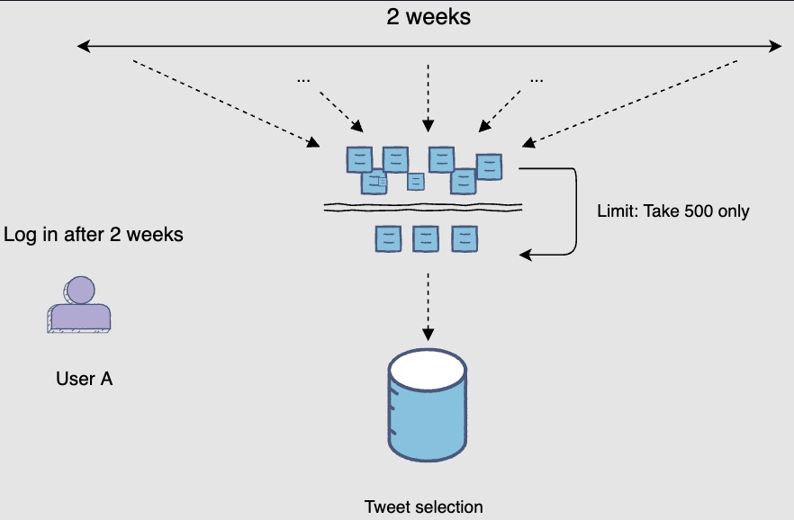
- Consider a scenario, where user A might log in after two weeks. A lot of posts would have been generated since A’s last login. Therefore, the post selection component will impose a limit on the post data it will select. Let’s assume that the limit is five-hundred. Now the selected five-hundred posts may have been generated over the last two days or throughout the two weeks, depending on the user’s network activity.
- The main idea is that the pool of posts keeps on increasing so a limit needs to be imposed on the number of posts that the component will fetch.
Network posts + interest / popularity-based posts
- The best retrieval system focus on fetching posts from both sources: (i) posts that align with a user’s taste, and (ii) posts that are trending. So taste and trend are the two areas to look out for, for any successful retrieval system.
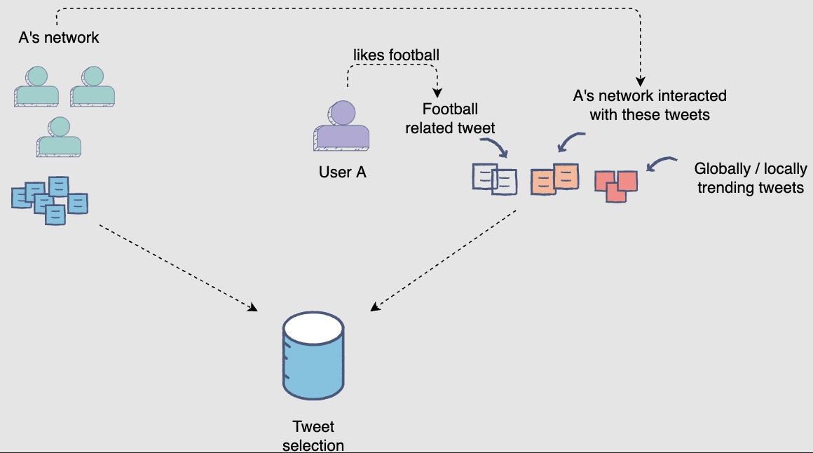
- Until now, the post selection component was only fetching posts from user A’s network of followees. However, there could be posts outside of user A’s network that have a high potential of engaging them. Hence, we arrive at a two-dimensional scheme of selecting network posts and potentially engaging posts.
- An engaging post could be one that:
- aligns with user A’s interests
- is locally/globally trending
- engages user A’s network
- The following diagram shows selection of network posts and interest/popularity-based posts:
- Selecting these posts can prove to be very beneficial in two cases:
- The user has recently joined the platform and follows only a few others. As such, their small network is not able to generate a sufficient number of posts for the post selection component (known as the Bootstrap problem).
- The user likes a post from a person outside of his network and decides to add them to their network. This would increase the discoverability on the platform and help grow the user’s network.
All of the schemes we have discussed showcase the dynamic nature of the post selection component’s task. The posts it will select will continue to change each time.
Ranker
-
The ranker component will receive the pool of selected posts and predict their probability of engagement. The posts will then be ranked according to their predicted engagement probabilities for display on user A’s feed. If we zoom into this component, we can:
- Train a single model to predict the overall engagement on the post.
- Train separate models. Each model can focus on predicting the occurrence probability of a certain user action for the post. There will be a separate predictor for like, comment, time spent, share, hide, and report. The results of these models can be merged, each having a different weight/importance, to generate a rank score. The posts will then be ranked according to this score.
-
The following illustration gives an idea of how the ranker component combines the outputs of different predictors with weights according to importance of user action in order to come up with a rank score for a post.
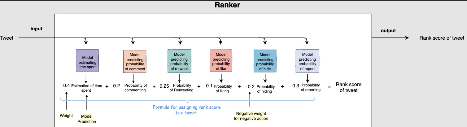
- Separately predicting each user action allows us to have greater control over the importance we want to give to each action when calculating the rank of the post. We can tweak the weights to display posts in such a manner that would align with our current business objectives, i.e., give certain user actions higher/lower weight according to the business needs.
Feature Engineering
-
The machine learning model is required to predict user engagement on user A’s Facebook feed. Let’s engineer features to help the model make informed predictions for the post ranking model.
-
Let’s begin by identifying the four main actors in a Facebook feed:
- The logged-in user.
- The user’s context
- The post
- The post’s author
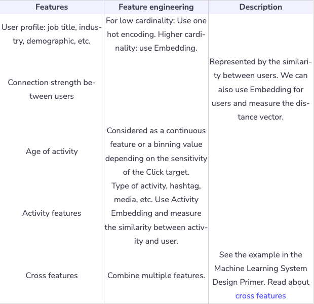
- Now it’s time to generate features based on these actors and their interactions. A subset of the features in each training data row is shown below.
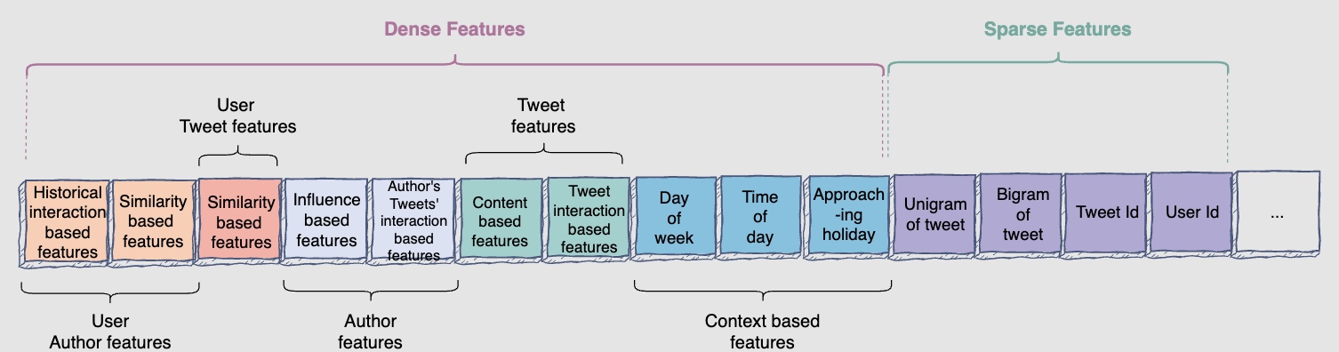
- Let’s discuss these features one by one. Note that we have marked sparse features with a tag.
User features
-
These features are based on the user.
-
user_age: The user’s age to filter out posts based on age restrictions. -
gender: The model will learn about gender-based preferences and recommend media accordingly. -
language: This feature will record the language of the user. It may be used by the model to see if a movie is in the same language that the user speaks. -
current_user_location: The current user location can help us show relevant content. For example, a person may go to San Francisco where a festival is happening (it is the talk of the town). Based on what is popular in a certain area where the user is located, you can show relevant posts.
-
Context-based features
-
These features are based on the user’s ‘context.
-
time_of_day: Noting the time of the day (coupled with the day of the week) can provide useful information. For example, if a user logs-in on a Monday morning, it is likely that they are at their place of work. Now, it would make sense to show shorter posts that they can quickly read. In contrast, if they login in the evening, they are probably at their home and would have more time at their disposal. Therefore, you can show them longer posts with video content as well, since the sound from the video would not be bothersome in the home environment. -
day_of_week: The day of the week can affect the type of post content a user would like to see on their feed. -
season_of_the_year: User’s viewing preference for different post topics may be patterned according to the four seasons of the year. -
lastest_k_tag_interactions: You can see the latest “k” tags included in the posts a user has interacted with to gain valuable insights. For example, assume that the last \(k = 5\) posts a user interacted with contain the tag “Solar eclipse”. From this, we can discern that the user is most likely interested in seeing posts centered around the solar eclipse. -
days_to_upcoming_holidayorapproaching_holiday: Recording the approaching holiday will allow the model to start showing the user more content centred around that holiday. For instance, if Independence Day is approaching, posts with more patriotic content would be displayed. -
device: It can be beneficial to observe the device on which the person is viewing content. A potential observation could be that users tend to view posts/content for shorter periods on their mobile when they are busy. Hence, we can recommend shorter posts when a user logs in from their mobile device and longer posts when they log in from their computer.
-
Post features
- These features are based on the post itself.
Features based on post’s content
- These features are based on the post’s content.
posts_id: (Sparse) This feature is used to identify posts that have high engagement and hence have a higher probability of engaging users.post_length: The length of the post positively correlates with user engagement, especially likes and reshares. It is generally observed that people have a short attention span and prefer a shorter read. Hence, a more concise post generally increases the chance of getting a like by the user. Also, we know that Facebook restricts the length of the post. So, if a person wants to share a post that has nearly used up the word limit, the person would not be able to add their thoughts on it, which might be off-putting.post_recency: The recency of the post is an important factor in determining user engagement, as people are most interested in the latest developments.is_image_video: The presence of an image or video makes the post more catchy and increases the chances of user engagement.is_URL: The presence of a URL may mean that the post:- Calls for action
- Provides valuable information
- Hence, such a post might have a higher probability of user engagement.
unigrams/bigramsof a post: (Sparse) The presence of certain unigrams or bigrams may increase the probability of engagement for a post. For example, during data visualisation, you may observe that posts with the bigram “Order now” have higher user engagement. The reason behind this might be that such posts are useful and informative for users as they redirect them towards websites where they can purchase things according to their needs.
Features based on post’s interaction
- You should also utilize the post’s interactions as features for our model. Posts with a greater volume of interaction have a higher probability of engaging the user. For instance, a post with more likes and comments is more relevant to the user, and there is a good chance that the user will like or comment on it too.
num_total_interactions: The total number of interactions (likes, comments and reshares) on a post can be used as a feature.- Caveat: Simply using these interactions as features might give an incomplete picture. Consider a scenario where Bill Gates posted a month ago, and his post received five million engagements over this period. Whereas, another post posted just an hour ago has two-thousand engagements and has become a trending post. Now, if your feature is based on the interaction count only, Bill Gates’s post would be considered more relevant, and the quick rise in the popularity of the trending post would not be given its due importance.
- To remedy this, we can apply a simple time-decay model to down-weigh the older interactions vs. the latest interactions. In other words, weigh latest interactions more than the ones that happened some time ago.
Time decay can be used in all features where there is a decline in the value of a quantity over time.
- One simple model can be to weight every interaction (like, comment, and share) by \(\frac{1}{t+1}\) where \(t\) is the number of days from current time.
- In the above scenario, you saw two posts, posted with a lot of time difference. The same scenario can also happen for two posts posted at the same time, as shown below. Let’s see how you can use time decay to see the real value of engagement on these posts.
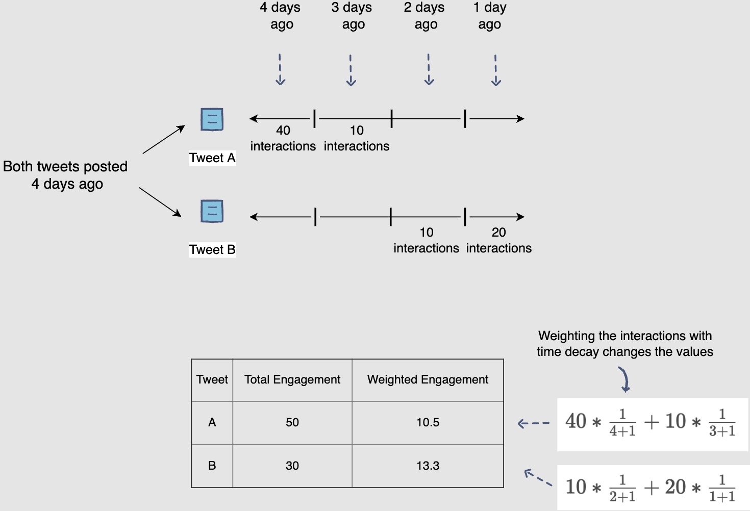
- Post A had a total of fifty interactions, while post B had a total of thirty. However, the interactions on post B were more recent. So, by using time decay, the weighted number of likes on post B became greater than those for post A.
- Another remedy is to use different time windows to capture the recency of interactions while looking at their numbers. The interaction in each window can be used as a feature. The figure below shows the different overlapping time windows to capture interactions on posts:
interactions_in_last_1_hourinteractions_in_last_1_dayinteractions_in_last_3_daysinteractions_in_last_week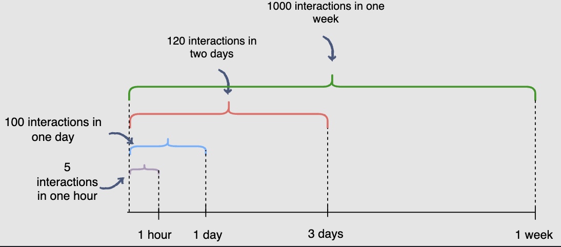
- To remedy this, we can apply a simple time-decay model to down-weigh the older interactions vs. the latest interactions. In other words, weigh latest interactions more than the ones that happened some time ago.
- Caveat: Simply using these interactions as features might give an incomplete picture. Consider a scenario where Bill Gates posted a month ago, and his post received five million engagements over this period. Whereas, another post posted just an hour ago has two-thousand engagements and has become a trending post. Now, if your feature is based on the interaction count only, Bill Gates’s post would be considered more relevant, and the quick rise in the popularity of the trending post would not be given its due importance.
Separate features for different engagements
- Previously, we discussed combining all interactions. You can also keep them as separate features, given you can predict different events, e.g., the probability of likes, shares and comments. Some potential features can be:
likes_in_last_3_dayscomments_in_last_1_dayreshares_in_last_2_hours
- The above three features are looking at their respective forms of interactions from all Facebook users. Another set of features can be generated by looking at the interactions on the post made only by user A’s network. The intuition behind doing this is that there is a high probability that if a post has more interactions from A’s network, then A, having similar tastes, will also interact with that post.
- The set of features based on user’s network’s interactions would then be:
likes_in_last_3_days_user’s_network_onlycomments_in_last_1_day_user’s_network_onlyreshares_in_last_2_hours_user’s_network_only
Author features
- These features are based on post’s author.
Author’s degree of influence
- A post written by a more influential author may be more relevant. There are several ways to measure the author’s influence. A few of these ways are shown as features for the model, below.
author_id: (Sparse) This is a very simple feature used to identify users with very high engagement rates, such as celebrities and influencers.is_author_verified: (Sparse) If an author is verified, it is highly likely that they are somebody important, and they have influence over people.author_num_followers: One important feature could be the number of followers the author has. Different inferences can be drawn from different follower counts, as shown below: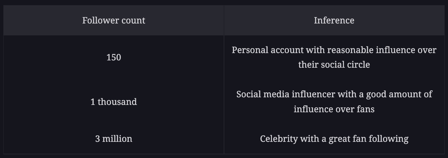
Normalised author_num_followers: You can observe a lot of variation in the follower counts of Facebook users. To bring each user’s follower count in a specific range, let’s say zero to ten-thousand, you can divide their follower count by the maximum observed follower count (across the platform) and then multiply it with ten-thousand.
follower_to_following_ratio: When coupled with the number of followers, the follower to following ratio can provide significant insight, regarding:- The type of user account
- The account’s influence
- The quality of the account’s content (posts)
- Let’s see how.

- Let’s see how.
author_social_rank: The idea of the author’s social_rank is similar to Google’s page rank. To compute the social rank of each user, you can do a random walk (like in page rank). Each person who follows the author contributes to their rank. However, the contribution of each user is not equal. For example, a user adds more weight if they are followed by a popular celebrity or a verified user.
Historical trend of interactions on the author’s posts
- Another very important set of features is the interaction history on the author’s posts. If historically, an author’s posts garnered a lot of attention, then it is highly probable that this will happen in the future, too.
A high rate of historical interaction for a user implies that the user posts high-quality content.
- Some features to capture the historical trend of interactions for the author’s posts are as follows:
author_engagement_rate_3months: The engagement rate of the historical posts by the author can be a great indicator of future post engagement. To compute the engagement rate in the last three months, we look at how many times different users interacted with the author’s posts that they viewed. \(\text { Engagement rate: } \frac{\text { post-interactions }}{\text { post-views }}\)author_topic_engagement_rate_3months: The engagement rate can be different based on the post’s topic. For example, if the author is a sports celebrity, the engagement rate for their family-related posts may be different from the engagement rate for their sports-related posts.- We can capture this difference by computing the engagement rate for the author’s posts per topic. Post topics can be identified in the following two ways:
- Deduce the post topic by the hashtags used
- Predict the post topic based on its content
These features don’t necessarily have to be based on data from three months, but rather you should utilize different time ranges, e.g., historical engagement rates in last week, month, three months, six months, etc.
Cross features
User-author features
-
These features are based on the logged-in user and the post’s author. They will capture the social relationship between the user and the author of the post, which is an extremely important factor in ranking the author’s posts. For example, if a post is authored by a close friend, family member, or someone that user is highly influenced by, there is a high chance that the user would want to interact with the post.
-
How can you capture this relationship in your signals given users are not going to specify them explicitly? Following are a few features that will effectively capture this.
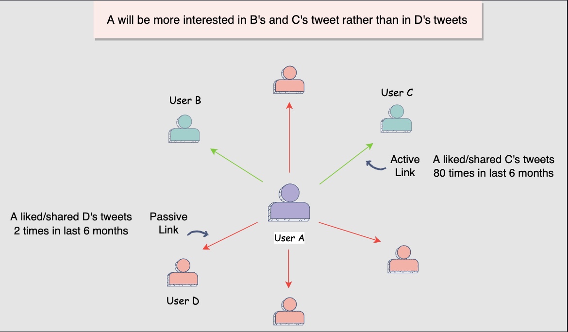
User-author historical interactions
- When judging the relevance of a post for a user, the relationship between the user and the post’s author plays an important role. It is highly likely that if the user has actively engaged with a followee in the past, they would be more interested to see a post by that person on their feed.
-
Few features based on the above concept can be:
-
author_liked_posts_3months: This considers the percentage of an author’s posts that are liked by the user in the last three months. For example, if the author created twelve posts in the last three months and the user interacted with six of these posts then the feature’s value will be: \(\frac{6}{12}=0.5 \text { or } 50 \%\). This feature shows a more recent trend in the relationship between the user and the author. -
author_liked_posts_count_1year: This considers the number of an author’s posts that the user interacted with, in the last year. This feature shows a more long term trend in the relationship between the user and the author.
-
Ideally, we should normalize the above features by the total number of posts that the user interacted with during these periods. This enables the model to see the real picture by cancelling out the effect of a user’s general interaction habits. For instance, let’s say user A generally tends to interact (e.g., like or comment) more while user B does not. Now, both user A and B have a hundred interactions on user C’s posts. User B’s interaction is more significant since they generally interact less. On the other hand, user A’s interaction is mostly a result of their tendency to interact more.
User-author similarity
-
Another immensely important feature set to predict user engagement focuses on figuring out how similar the logged-in user and the post’s author are. A few ways to compute such features include:
common_followees: This is a simple feature that can show the similarity between the user and the author. For a user-author pair, you will look at the number of users and hashtags that are followed by both the user and the author.
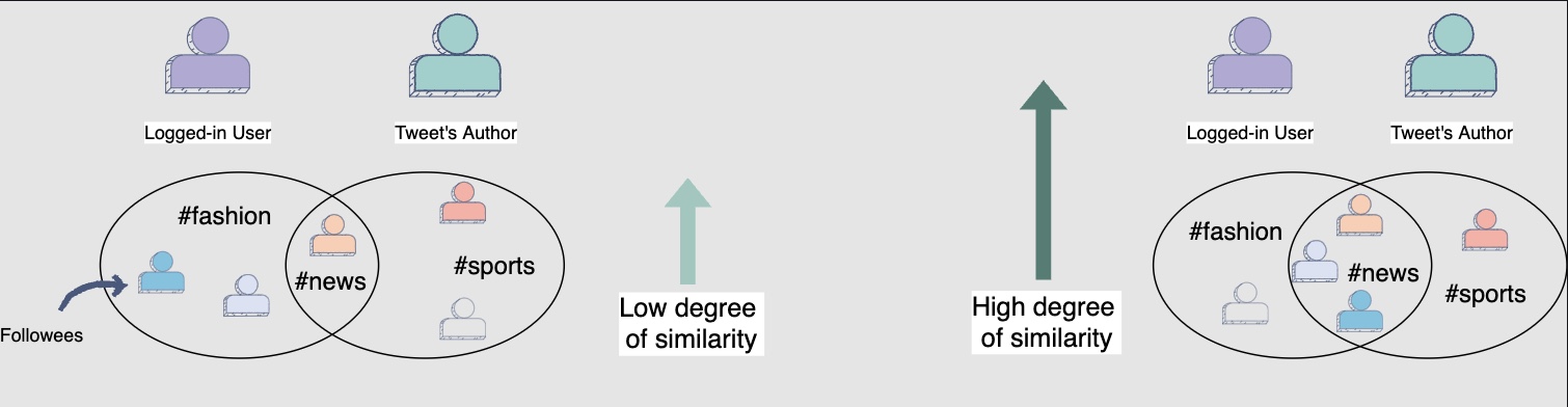
topic_similarity: The user and author similarity can also be judged based on their interests. You can see if they interact with similar topics/hashtags. A simple method to check this is the TF-IDF based similarity between the hashtags:- followed by the logged-in user and author
- present in the posts that the logged-in user and author have interacted with in the past
- used by the author and logged-in user in their posts
- The similarity between their search histories on Facebook can also be used for the same purpose.
-
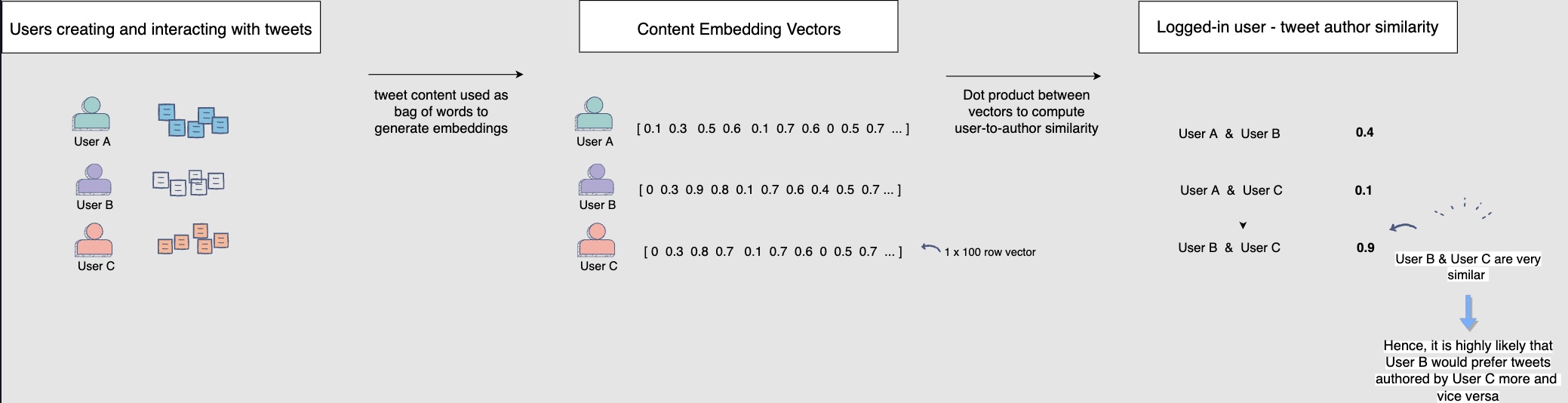
post_content_embedding_similarity: Each user is represented by the content that they have generated and interacted with in the past. You can utilize all of that content as a bag-of-words and build an embedding for every user. With an embedding vector for each user, the dot product between them can be used as a fairly good estimate of user-to-author similarity.Embedding helps to reduce the sparsity of vectors generated otherwise.
- Content embedding similarity between logged-in user and post’s author. The following diagram shows that users B and C are very similar. Hence, it is highly likely that user B will prefer posts authored by user C more and vice versa:
- Content embedding similarity between logged-in user and post’s author. The following diagram shows that users B and C are very similar. Hence, it is highly likely that user B will prefer posts authored by user C more and vice versa:
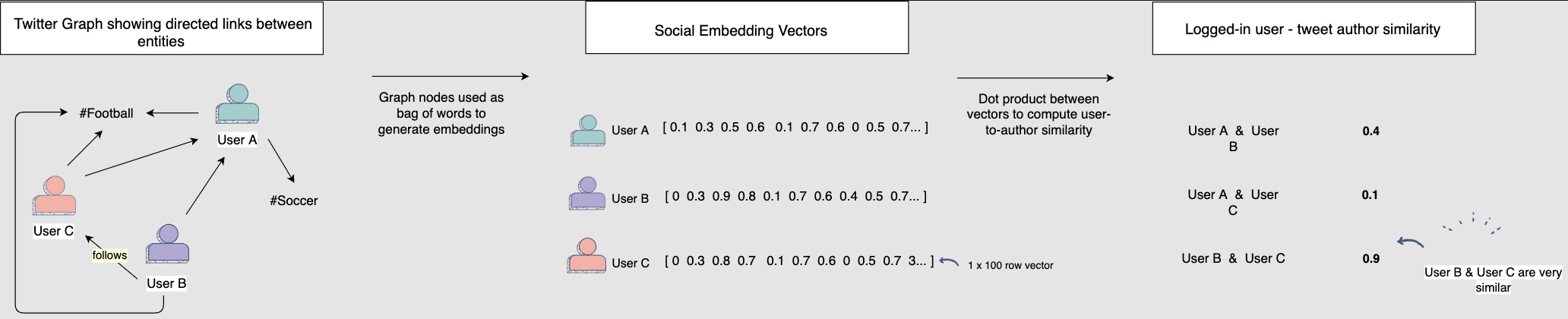
social_embedding_similarity: Another way to capture the similarity between the user and the author is to generate embeddings based on the social graph rather than based on the content of posts, as we discussed earlier. The basic notion is that people who follow the same or similar topics or influencers are more likely to engage with each other’s content. A basic way to train this model is to represent each user with all the other users and topics (user and topic ids) that they follow in the social graph. Essentially, every user is represented by bag-of-ids (rather than bag-of-words), and you use that to train an embedding model. The user-author similarity will then be computed between their social embeddings and used as a signal. Social similarity between user and author:
User-post features
- The similarity between the user’s interests and the post’s topic is also a good indicator of the relevance of a post. For instance, if user A is interested in football, a post regarding football would be very relevant to them.
topic_similarity: You can use the hashtags and/or the content of the posts that the user has either posted or interacted with, in the last six months and compute the TF-IDF similarity with the post itself. This indicates whether the post is based on a topic that the user is interested in.embedding_similarity: Another option to find the similarity between the user’s interest and the post’s content is to generate embeddings for the user and the post. The post’s embedding can be made based on the content and hashtags in it. While the user’s embedding can be made based on the content and hashtags in the posts that they have written or interacted with. A dot product between these embeddings can be calculated to measure their similarity. A high score would equate to a highly relevant post for a user.
Training Data Generation
- Before building any ML models we need to collect training data. The goal is to collect data across different types of posts, while simultaneously improving user experience. Below are some of the ways we can collect training data:
- Rank by chronicle order: This approach ranks each post in chronological order. Use this approach to collect click/not-click data. The trade-off here is serving bias because of the user’s attention on the first few posts. Also, there is a data sparsity problem because different activities, such as job changes, rarely happen compared to other activities on LinkedIn.
- Random serving: This approach ranks post by random order. This may lead to a bad user experience. It also does not help with sparsity, as there is a lack of training data about rare activities.
- Use a Feed Ranking algorithm: This would rank the top feeds. Within the top feeds, you would permute randomly. Then, use the clicks for data collection. This approach provides some randomness and is helpful for models to learn and explore more activities.
- Based on this analysis, we will use an algorithm to generate training data so that we can later train a machine learning model.
-
We can start to use data for training by selecting a period of data: last month, last 6 months, etc. In practice, we want to find a balance between training time and model accuracy. We also downsample the negative data to handle the imbalanced data.
- Your user engagement prediction model’s performance will depend largely on the quality and quantity of the training data. So, let’s see how you can generate training data for your model.
Note that the term training data row and training example will be used interchangeably.
Training data generation through online user engagement
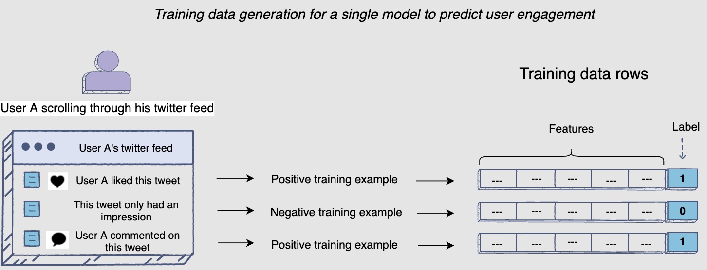
- The users’ online engagement with posts can give us positive and negative training examples. For instance, if you are training a single model to predict user engagement, then all the posts that received user engagement would be labeled as positive training examples. Similarly, the posts that only have impressions would be labeled as negative training examples.
Impression: If a post is displayed on a user’s Facebook feed, it counts as an impression. It is not necessary that the user reads it or engages with it, scrolling past it also counts as an impression.
- The following diagram shows that any user engagement counts as positive example:
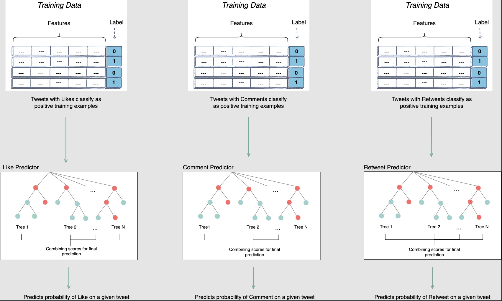
- However, as you saw in the architectural components lesson, that you can train different models, each to predict the probability of occurrence of different user actions on a post. The following illustration shows how the same user engagement (as above) can be used to generate training data for separate engagement prediction models.
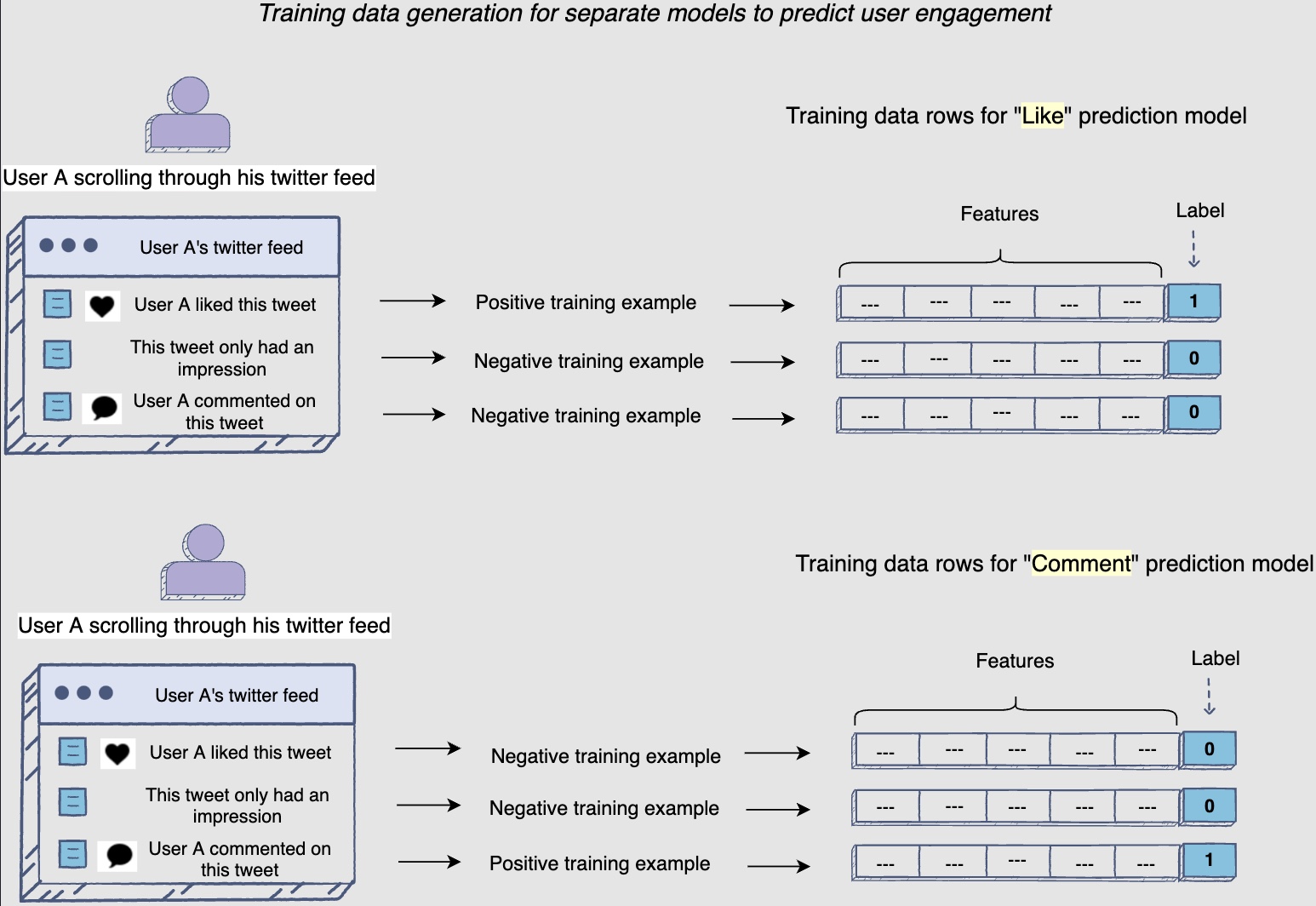
- When you generate data for the “Like” prediction model, all posts that the user has liked would be positive examples, and all the posts that they did not like would be negative examples.
Note how the comment is still a negative example for the “Like” prediction model.
- Similarly, for the “Comment” prediction model, all posts that the user commented on would be positive examples, and all the ones they did not comment on would be negative examples.
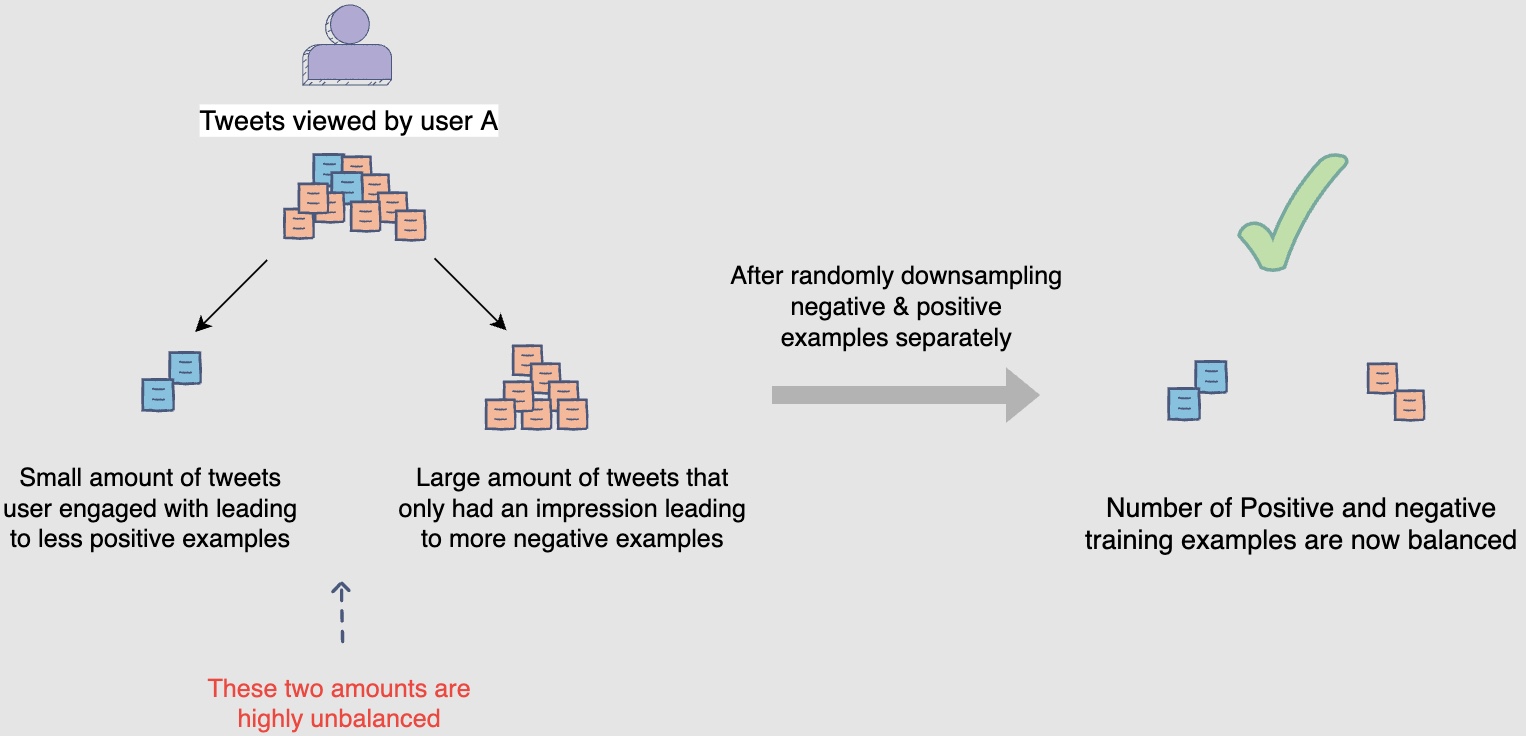
Balancing positive and negative training examples by randomly downsampling
-
Models essentially learn behavior from the data we present them with. Therefore, it’s important for us to provide a good sample of both positive and negative examples to model these interactions between different actors in a system. In the feed-based system scenario, on average, a user engages with as little as approximately 5% of the posts that they view per day. How would this percentage affect the ratio of positive and negative examples on a larger scale? How can this be balanced?
-
Looking at the bigger picture, assume that one-hundred million posts are viewed collectively by the users in a day. With the 5% engagement ratio, you would be able to generate five million positive examples, whereas the remaining ninety-five million would be negative.
-
Let’s assume that you want to limit your training samples to ten million, given that the training time and cost increases as training data volume increases. If you don’t do any balancing of training data and just randomly select ten million training samples, your models will see only 0.5 million positive examples and 9.5 million negative examples. In this scenario, the models might not be able to learn key positive interactions.
-
Therefore, in order to balance the ratio of positive and negative training samples, you can randomly downsample:
- negative examples to five million samples
- positive examples to five million samples
-
Now, you would have a total of ten million training examples per day; five million of which are positive and five million are negative.
Note: If a model is well-calibrated, the distribution of its predicted probability is similar to the distribution of probability observed in the training data. However, as we have changed the sampling of training data, our model output scores will not be well-calibrated. For example, for a post that got only 5% engagement, the model might predict 50% engagement. This would happen because the model is trained on data that has an equal quantity of negative and positive samples. So the model would think that it is as likely for a post to get engagement as it is to be ignored. However, we know from the training that this is not the case. Given that the model’s scores are only going to be used to rank posts among themselves, poor model calibration doesn’t matter much in this scenario. We will discuss this in the ads system chapter, where calibrated scores are important, and we need to be mindful of such a sampling technique.
Train test split
-
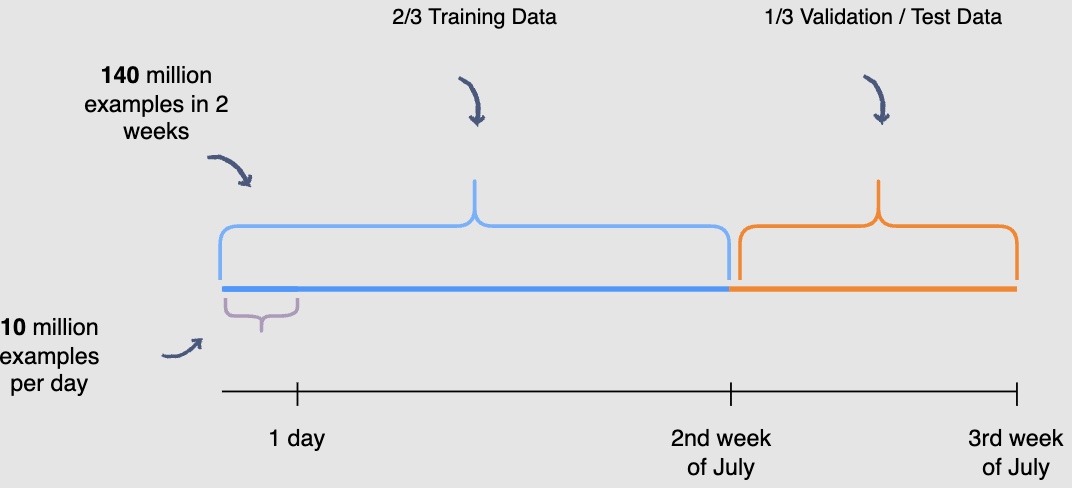
You need to be mindful of the fact that the user engagement patterns may differ throughout the week. Hence, you will use a week’s engagement to capture all the patterns during training data generation. At this rate, you would end up with around seventy million rows of training data.
-
You may randomly select \(\frac{2}{3}^{rd}\) or 66.6% , of the seventy million training data rows that you have generated and utilize them for training purposes. The rest of the \(\frac{1}{3}^{rd}\) or 33.3%, can be used for validation and testing of the model. However, this random splitting defeats the purpose of training the model on an entire week’s data. Also, the data has a time dimension, i.e., we know the engagement on previous posts, and we want to predict the engagement on future posts ahead of time. Therefore, you will train the model on data from one time interval and validate it on the data with the succeeding time interval. This will give a more accurate picture of how the model will perform in a real scenario.
We are building models with the intent to forecast the future.
- In the following illustration, we are training the model using data generated from the first and second week of July and data generated in the thirdweek of July for validation and testing purposes. THe following diagram indicates the splitting data procedure for training, validation, and testing:
- Possible pitfalls seen after deployment where the model is not offering predictions with great accuracy (but performed well on the validation/test splits): Question the data. Garbage in - Garbage out. The model is only as good as the data it was trained on. Data drifts where the real-world data follows a different distribution that the model was trained on are fairly common.
- When was the data acquired? The more recent the data, better the performance of the model.
- Does the data show seasonality? i.e., we need to be mindful of the fact that the user engagement patterns may differ throughout the week. For e.g., don’t use data from weekdays to predict for the weekends.
- Was the data split randomly? Random splitting defeats the purpose since the data has a time dimension, i.e., we know the engagement on previous posts, and we want to predict the engagement on future posts ahead of time. Therefore, you will train the model on data from one time interval and validate it on the data with the succeeding time interval.
Ranking: Modeling
-
In this lesson, we’ll explore different modeling options for the post ranking problem.
-
In the previous lesson, you generated the training data. Now, the task at hand is to predict the probability of different engagement actions for a given post. So, essentially, your models are going to predict the probability of likes, comments and shares, i.e., P(click), P(comments) and P(share). Looking at the training data, we know that this is a classification problem where we want to minimize the classification error or maximize area under the curve (AUC).
Modeling options
- Some questions to consider are: Which model will work best for this task? How should you set up these models? Should you set up completely different models for each task? Let’s go over the modeling options and try to answer these questions. We will also discuss the pros and cons of every approach.
Logistic regression
-
Initially, a simple model that makes sense to train is a logistic regression model with regularization, to predict engagement using the dense features that we discussed in the feature engineering lesson.
-
A key advantage of using logistic regression is that it is reasonably fast to train. This enables you to test new features fairly quickly to see if they make an impact on the AUC or validation error. Also, it’s extremely easy to understand the model. You can see from the feature weights which features have turned out to be more important than others.
-
A major limitation of the linear model is that it assumes linearity exists between the input features and prediction. Therefore, you have to manually model feature interactions. For example, if you believe that the day of the week before a major holiday will have a major impact on your engagement prediction, you will have to create this feature in your training data manually. Other models like tree-based and neural networks are able to learn these feature interactions and utilize them effectively for predictions.
-
Another key question is whether you want to train a single classifier for overall engagement or separate ones for each engagement action based on production needs. In a single classifier case, you can train a logistic regression model for predicting the overall engagement on a post. Posts with any form of engagement will be considered as positive training examples for this approach.
-
Another approach is to train separate logistic regression models to predict P(like), P(comments) and P(share).
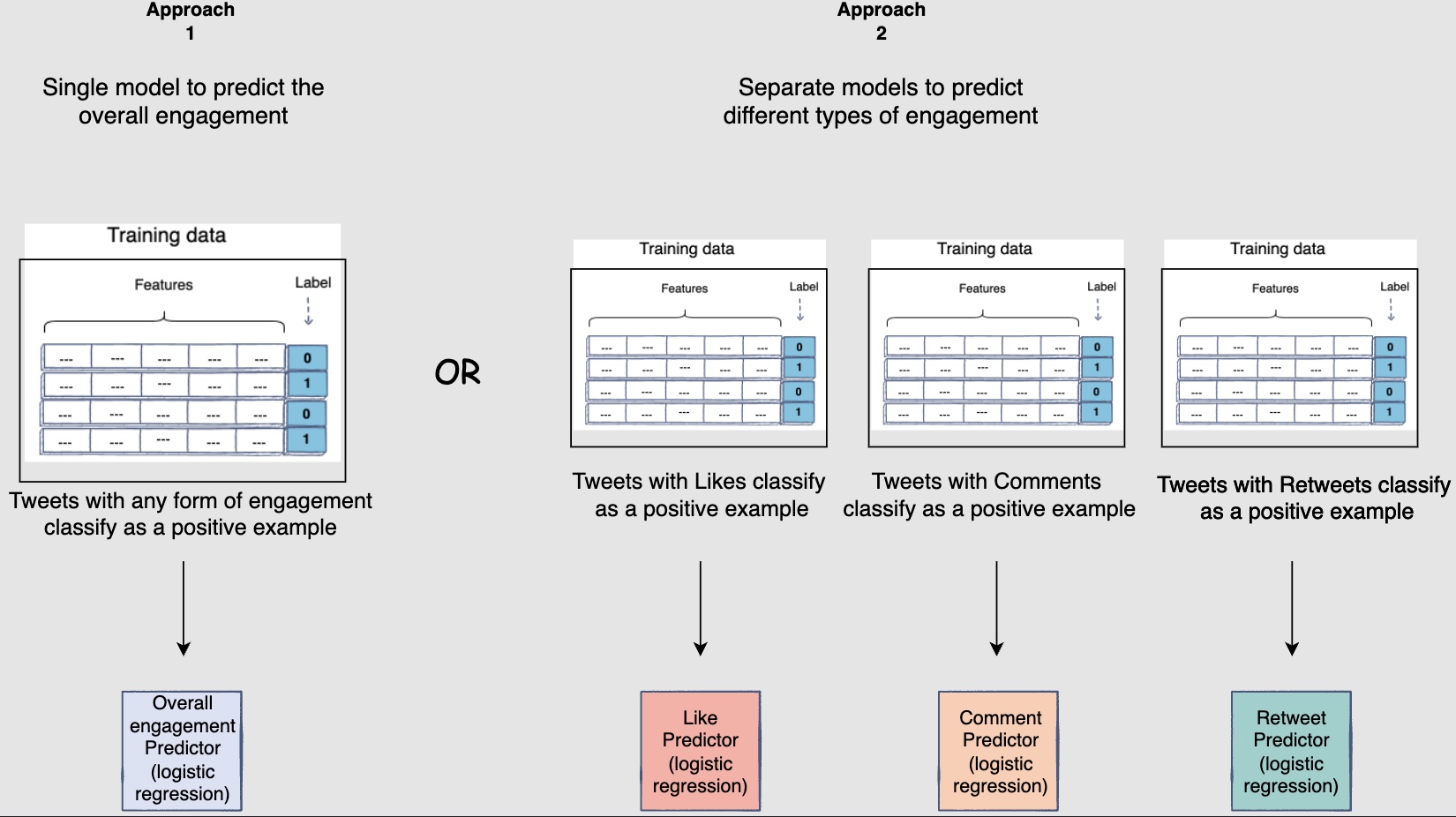
- These models will utilize the same features. However, the assignments of labels to the training examples will differ. Posts with likes, comments, or shares will be considered positive examples for the overall engagement predictor model. Only posts with likes will be considered as positive examples for the “Like” predictor model. Similarly, only posts with comments will be considered as positive examples for the “Comment” predictor model and only posts with shares will be considered as positive examples for the “share” predictor model.
As with any modelling, we should try and tune all the hyperparameters and play with different features to find the best model to fit this problem.
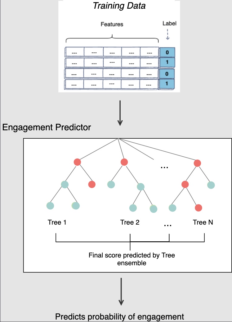
MART
-
MART stands for multiple additive regression trees.
-
Another modeling option that should be able to outperform logistic regression with dense features is additive tree-based models, e.g., Boosted Decision Trees and Random Forest. Trees are inherently able to utilize non-linear relations between features that aren’t readily available to logistic regression as discussed in the above section.
-
Tree-based models also don’t require a large amount of data as they are able to generalize well quickly. So, a few million examples should be good enough to give us an optimized model.
-
There are various hyperparameters that you might want to play around to get to an optimized model, including
- Number of trees
- Maximum depth
- Minimum samples needed for split
- Maximum features sampled for a split
-
To choose the best predictor, you should do hyperparameter tuning and select the hyperparameter that minimizes the test error.
Approach 1: Single model to predict the overall engagement
- A simple approach is to train a single model to predict the overall engagement.
Approach 2: Specialized predictor for each type of user engagement
- You could have specialized predictors to predict different kinds of engagement. For example, you can have a like predictor, a comment predictor and a reshare predictor. Once again these models will utilize the same features. However, the assignments of labels to the training examples will differ depending on the model’s objective.
Approach 3:
-
Consider a scenario, where a person reshares a post but does not click the like button. Even though the user didn’t actually click on the like button, shareing generally implies that the user likes the post. The positive training example for the share model may prove useful for the like model as well. Hence, you can reuse all positive training examples across every model.
-
One way to utilize the overall engagement data among each individual predictor of P(like), P(comment) and P(share) is to build one common predictor, i.e., P(engagement) and share its output as input into all of your predictors.
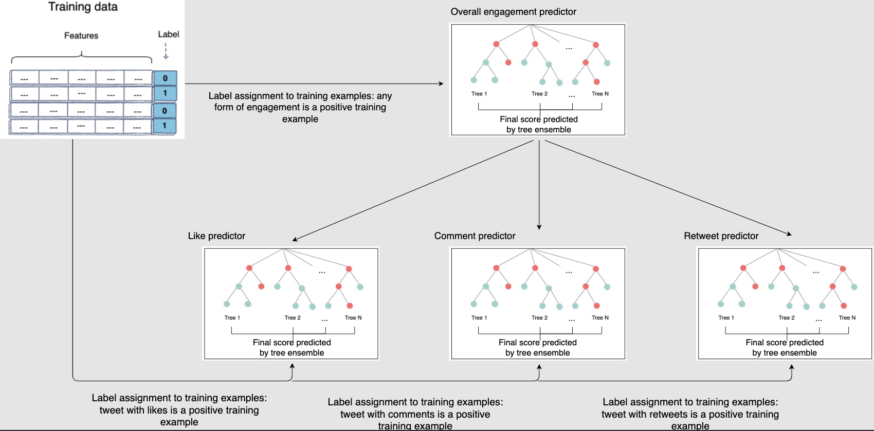
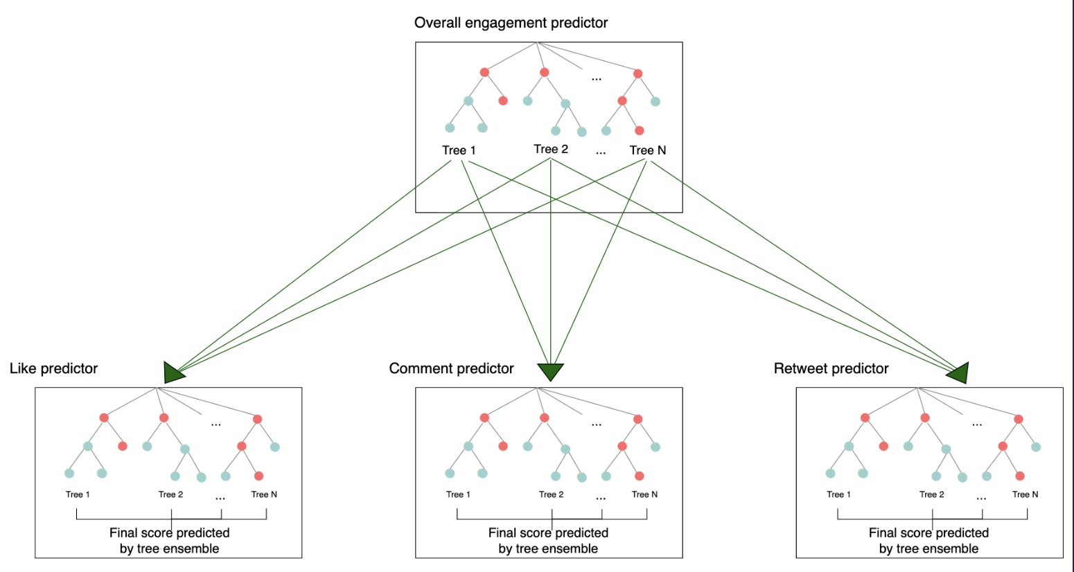
To take approach three a notch further, you can use the output of each tree in the “overall engagement predictor” ensemble as features in the individual predictors. This allows for even better learning as the individual model will be able to learn from the output of each individual tree.
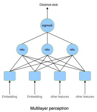
Deep learning: Stage 2 Ranking
-
With advancements in computational power and the amount of training data you can gather from hundreds of million users, deep learning can be very powerful in predicting user engagement for a given post and showing the user a highly personalized feed.
-
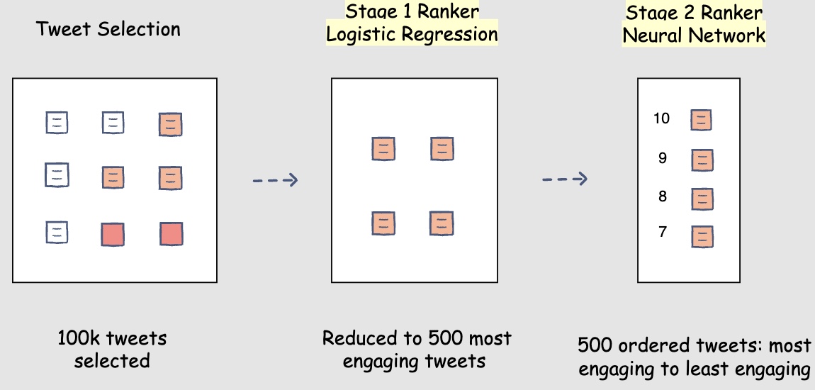
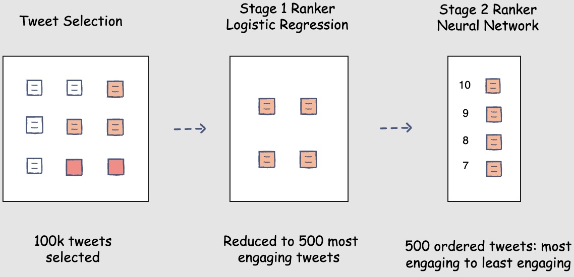
Having said that, training the model as well as evaluating the model at feed generation time can make this approach computationally very expensive. So, you may want to fall back to the multi-layer approach, which we discussed in the search ranking chapter, i.e., having a simpler model for stage one ranking and use complex stage two model to obtain the most relevant posts ranked at the top of the user’s Facebook feed. The following figure shows the layered model approach:
-
Like with the tree-based approach, there are quite a few hyperparameters that you should tune for deep learning to find the most optimized model that minimizes the test set error. They are:
- Learning rate
- Number of hidden layers
- Batch size
- Number of epochs
- Dropout rate for regularizing model and avoiding overfitting
Neural networks are a great choice to add all the raw data and dense features that we used for tree-based models.
Separate neutral networks
- One way is to train separate neural nets for each of the P(like), P(comment) and P(share) as follows:
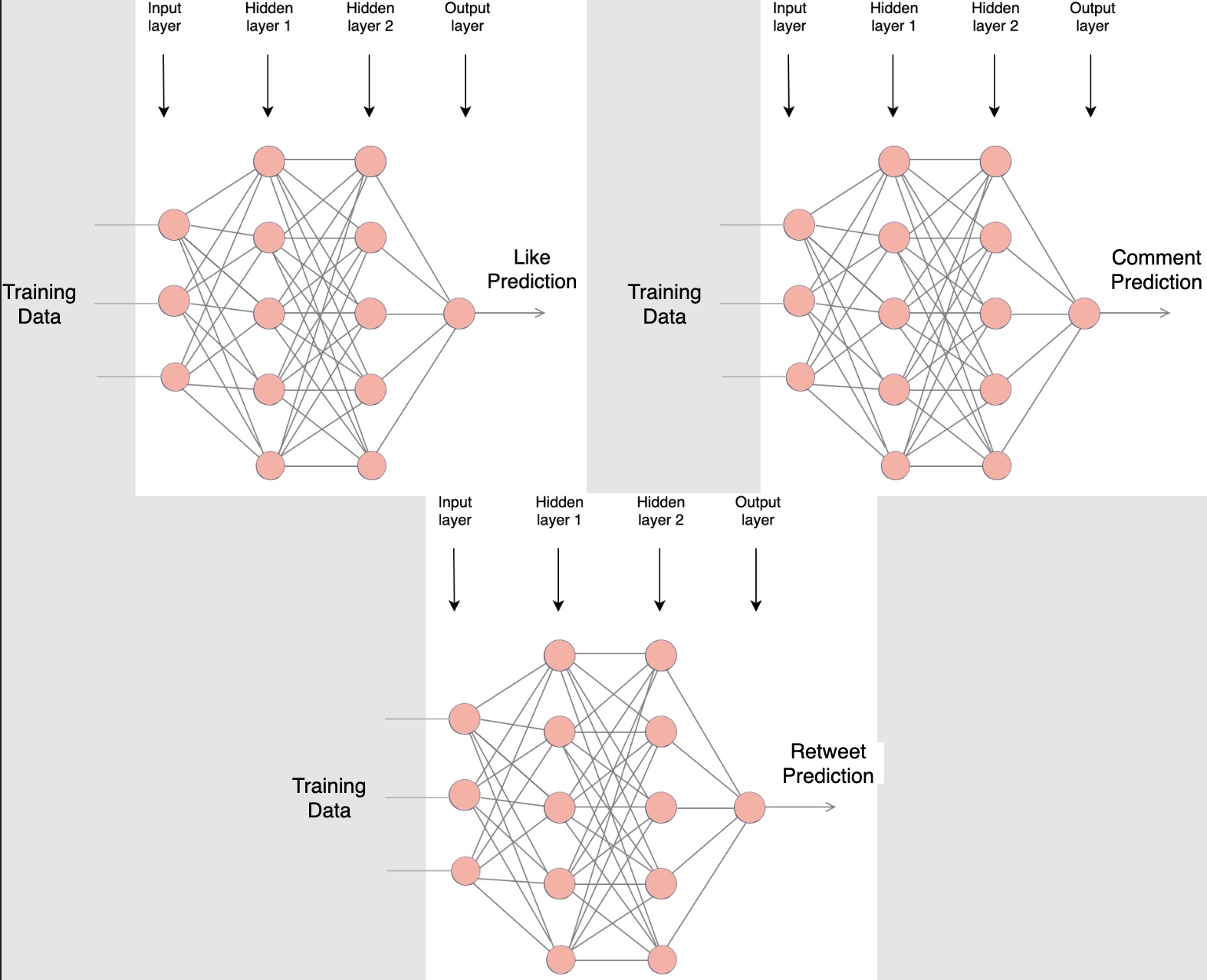
- However, for a very large scale data set, training separate deep neural networks (NNs) can be slow and take a very long time (ten’s of hours to days). The following approach of setting up the models for multi-task learning caters to this problem.
Multi-task neural networks
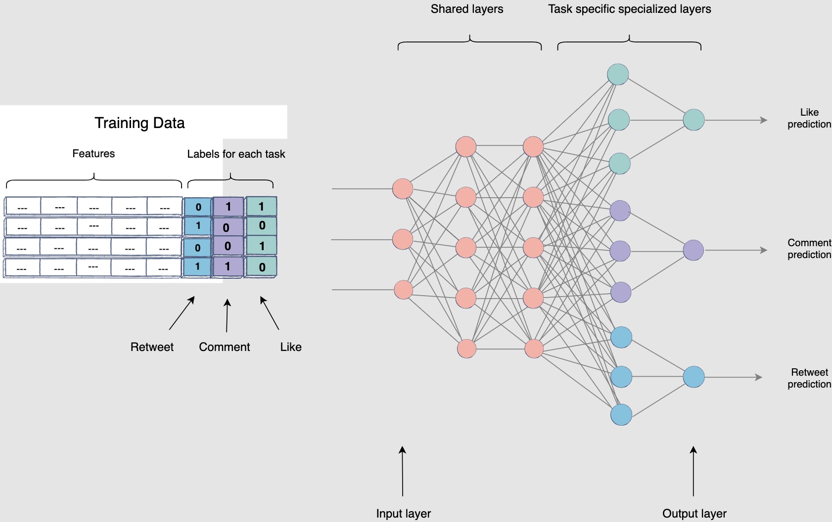
- Likes, comments, and shares are all different forms of engagement on a post. Therefore, predicting P(like), P(comment) and P (share) are similar tasks. When predicting similar tasks, you can use multitask learning. Referring back to the scenario in approach 3 of MART, if you want to predict the probability of a like, it would certainly be helpful for the model to know that this post has been shareed (knowledge sharing). Hence, you can train a neural network with shared layers (for shared knowledge) appended with specialized layers for each task’s prediction. The weights of the shared layers are common to the three tasks. Whereas in the task-specific layer, the network learns information specific to the tasks. The loss function for this model will be the sum of individual losses for all the tasks:
- The model will then optimize for this joint loss leading to regularization and joint learning.
Given the training time is slow for neural networks, training one model (shared layers) would make the overall training time much faster. Moreover, this will also allow us to share all the engagement data across each learning task. THe following diagram shows the multi-task neural network configuration where the specialized layers share the initial layers:
- This approach should be able to perform at least as effective as training separate networks for each task. It should be able to outperform in most cases as we use the shared data and use it across each predictor. Also, one key advantage of using shared layers is that models would be much faster to train than training completely separate deep neural networks for each task.
Stacking models and online learning
-
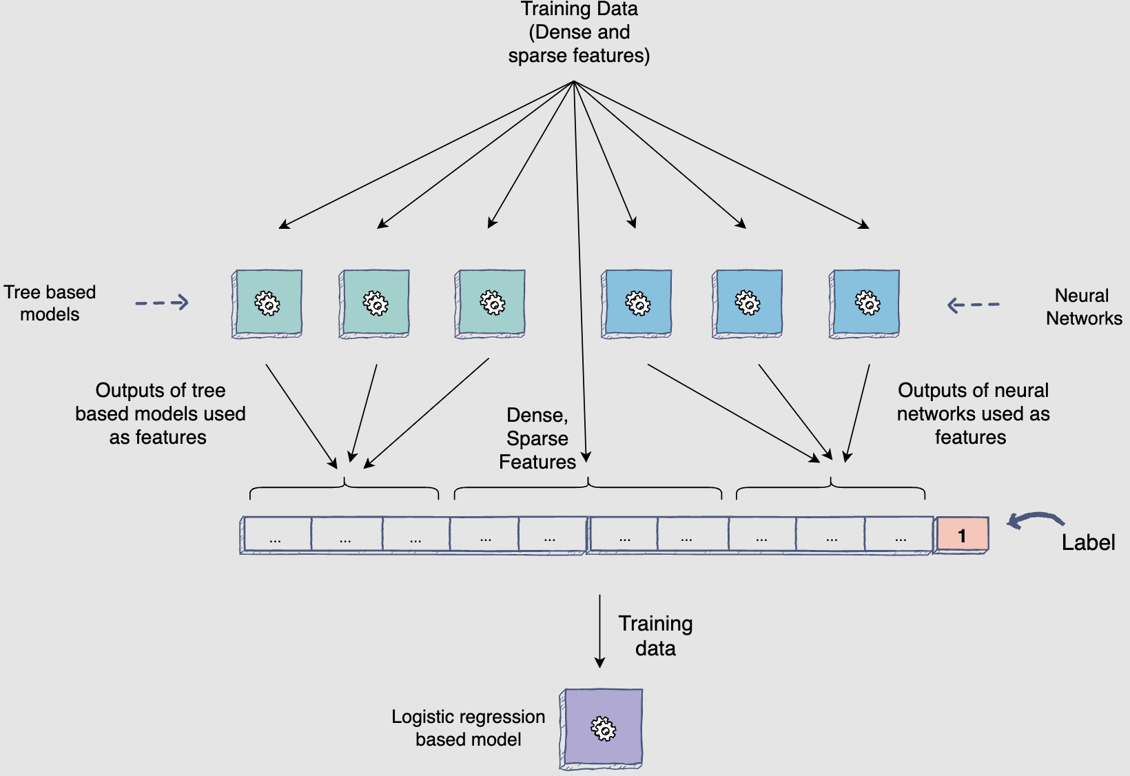
One way to outperform the “single model technique approach” is to use multiple models to utilize the power of different techniques by stacking models on top of each other. Let’s go over one such stacking setup that should work out very well for the feed problem.
-
The setup includes training tree-based models and neural networks to generate features that you will utilize in a linear model (logistic regression). The main advantage of doing this is that you can utilize online learning, meaning we can continue to update the model with every user action on the live site. You can also use sparse features in our linear model while getting the power of all non-linear relations and functions through features generated by tree-based models and neural networks.
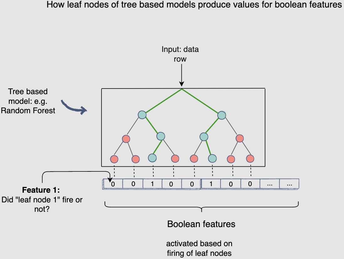
- For trees, you can generate features by using the triggering of leaf nodes, e.g., given two trees with four leaf nodes, each will result in eight features that can be used in logistic regression, as shown below. The following figure shows a tree based model generating features for the logistic regression model:
-
In the above diagram, each leaf node in the random forest will result in a boolean feature that will be active based on whether the leaf node is triggered or not.
-
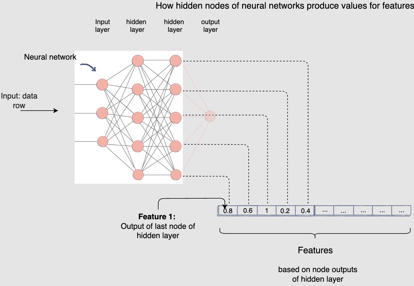
Similarly, for neutral networks, rather than predicting the probability of events, you can just plug-in the output of the last hidden layer as features into the logistic regression models. The following figure shows a neural network generating features for the logistic regression model:
- To summarize, this stacking model setup will still give us all the learning power of deep neural networks and tree-based models along with the flexibility of training logistic regressions model, while keeping it almost real-time refreshed with online learning.
Logistic regression can be easily used for changing the model online, based on real-time user interactions that happen with the posts. This helps the model to re-learn the weight of all tree leaves as well.
-
Another advantage of using real-time online learning with logistic regression is that you can also utilize sparse features to learn the interaction, e.g., features like user_id and post_id can be used to memorize the interaction with each individual user and post.
-
Given that features like post_id and user_id are extremely sparse, training and evaluation of the model must be done in a distributed environment because the data won’t fit on one machine.
Diversity/Re-ranking
- One of the inherent challenges with recommendation engines is that they can inadvertently limit your experience – what is sometimes referred to as a “filter bubble.” By optimizing for personalization and relevance, there is a risk of presenting an increasingly homogenous stream of videos. This is a concern that needs to be addressed when developing our recommendation system.
- Serendipity is important to enable users to explore new interests and content areas that they might be interested in. In isolation, the recommendation system may not know the user is interested in a given item, but the model might still recommend it because similar users are interested in that item (using collaborative filtering).
- Also, another important function of a diversifier/re-ranker is that it boosts the score of fresh content to make sure it gets a chance at propagation. Thus, freshness, diversity, and fairness are the three important areas this block addresses.
- Let’s learn methods to reduce monotony on the user’s Facebook feed.
Why do you need diverse posts?
- Diversity is essential to maintaining a thriving global community, and it brings the many corners of Facebook closer together. To that end, sometimes you may come across a post in your feed that doesn’t appear to be relevant to your expressed interests or have amassed a huge number of likes. This is an important and intentional component of our approach to recommendation: bringing a diversity of posts into your newsfeed gives you additional opportunities to stumble upon new content categories, discover new creators, and experience new perspectives and ideas as you scroll through your feed.
- By offering different videos from time to time, the system is also able to get a better sense of what’s popular among a wider range of audiences to help provide other Facebook users a great experience, too. Our goal is to find balance (exploitation v/s exploration tradeoff) between suggesting content that’s relevant to you while also helping you find content and creators that encourage you to explore experiences you might not otherwise see.
- Let’s assume that you adopted the following modelling option for your Facebook feed ranking system. The post selection component will select one-hundred thousand posts for user A’s Facebook feed. The stage one ranker will choose the top five-hundred most engaging posts for user A. The stage two ranker will then focus on assigning engagement probabilities to these posts with a higher degree of accuracy. Finally, the posts will be sorted according to the engagement probability scores and will be ready for display on the user’s Facebook feed.
-
Consider a scenario where the sorted list of posts has five consecutive posts by the same author. No, your ranking model hasn’t gone bonkers! It has rightfully placed these posts at the top because:
- The logged-in user and the post’s author have frequently interacted with each other’s posts
- The logged-in user and the post’s author have a lot in common like hashtags followed and common followees
- The author is very influential, and their posts generally gain a lot of traction
This scenario remains the same for any modelling option.
Safeguarding the viewing experience
- The newsfeed recommendation system should also be designed with safety as a consideration. Reviewed content found to depict things like graphic medical procedures or legal consumption of regulated goods, for example – which may be shocking if surfaced as a recommended video to a general audience that hasn’t opted in to such content – may not be eligible for recommendation.
- Similarly, videos that have explicitly disliked by the user, have just been uploaded or are under review, and spam content such as videos seeking to artificially increase traffic, also may be ineligible for recommendation into anyone’s newsfeed.
Interrupting repetitive patterns
- To keep your newsfeed interesting and varied, our recommendation system works to intersperse diverse types of content along with those you already know you love. For example, your newsfeed generally won’t show two videos in a row made with the same sound or by the same creator.
- Recommending duplicated content, content you’ve already seen before, or any content that’s considered spam is also not desired. However, you might be recommended a video that’s been well received by other users who share similar interests.
Diversity in posts’ authors
- However, no matter how good of a friend the author is or how interesting their posts might be, user A would eventually get bored of seeing posts from the same author repeatedly. Hence, you need to introduce diversity with regards to the posts’ author.
Diversity in posts’ content
- Another scenario where we might need to introduce diversity is the post’s content. For instance, if your sorted list of posts has four consecutive posts that have videos in them, the user might feel that their feed has too many videos.
Introducing the repetition penalty to interrupt repetitive patterns
-
To rid the Facebook feed from a monotonous and repetitive outlook, we will introduce a repetition penalty for repeated post authors and media content in the post.
-
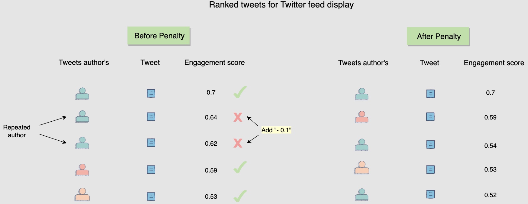
One way to introduce a repetition penalty could be to add a negative weight to the post’s score upon repetition. For instance, in the following diagram, whenever you see the author being repeated, you add a negative weight of -0.1 to the post’s score. The following figure shows a repetition penalty for repeated post author:
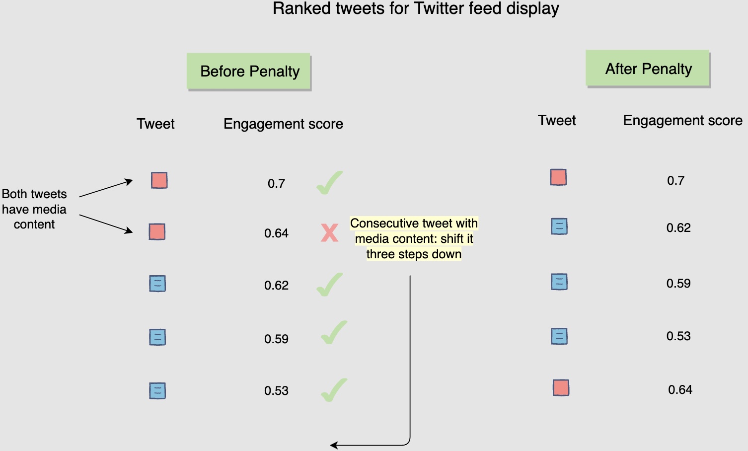
- Another way to achieve the same effect is to bring the post with repetition three steps down in the sorted list. For instance, in the following diagram, when you observe that two consecutive posts have media content in them, you bring the latter down by three steps. The following figure shows a repetition penalty for consecutive posts with media content:
Online Experimentation
-
Let’s see how to evaluate the model’s performance through online experimentation.
-
Let’s look at the steps from training the model to deploying it.
Step 1: Training different models
- Earlier, in the training data generation lesson, we discussed a method of splitting the training data for training and validation purposes. After the split, the training data is utilized to train, say, fifteen different models, each with a different combination of hyperparameters, features, and machine learning algorithms. The following figure shows different models are trained to predict user engagement:
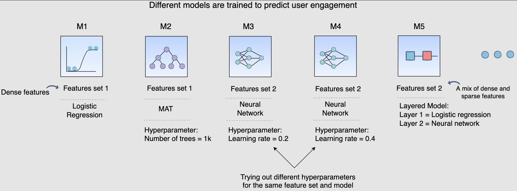
- The above diagram shows different models that you can train for our post engagement prediction problem. Several combinations of feature sets, modeling options, and hyperparameters are tried.
Step 2: Validating models offline
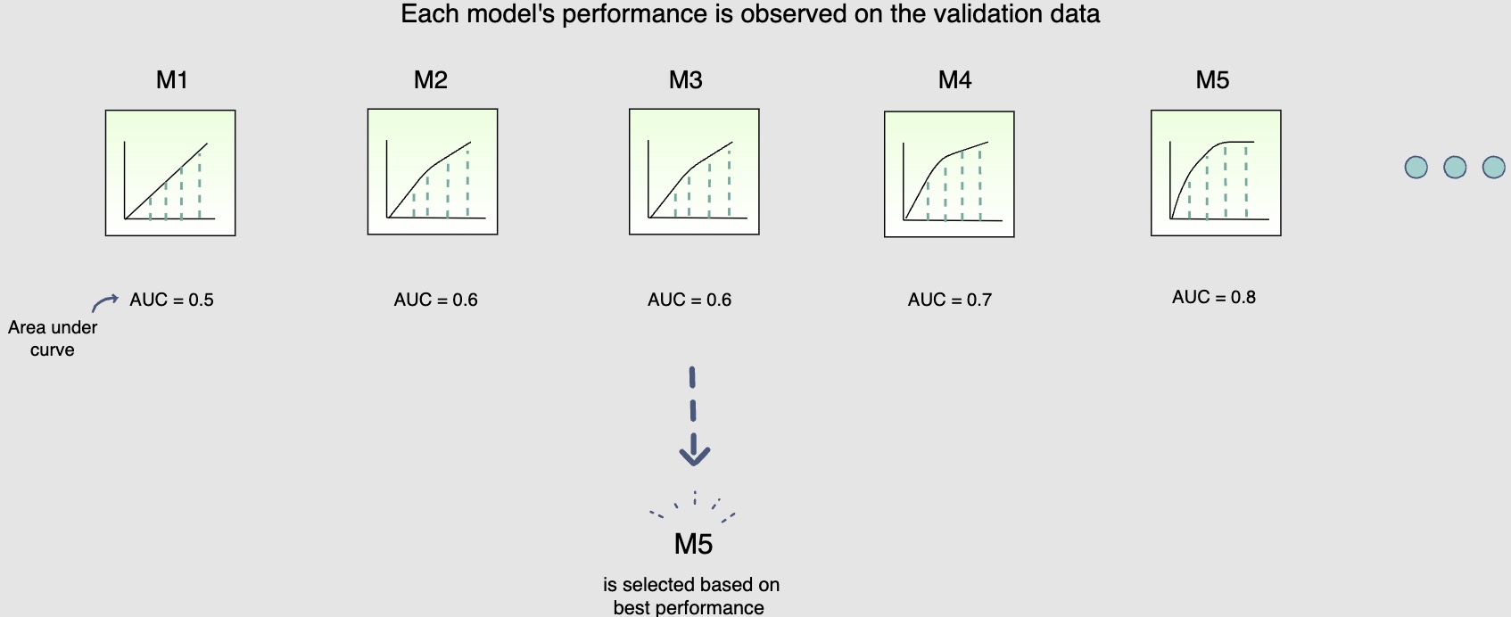
- Once these fifteen models have been trained, you will use the validation data to select the best model offline. The use of unseen validation data will serve as a sanity check for these models. It will allow us to see if these models can generalise well on unseen data. The following figure shows each model’s performance is observed on the validation data
Step 3: Online experimentation
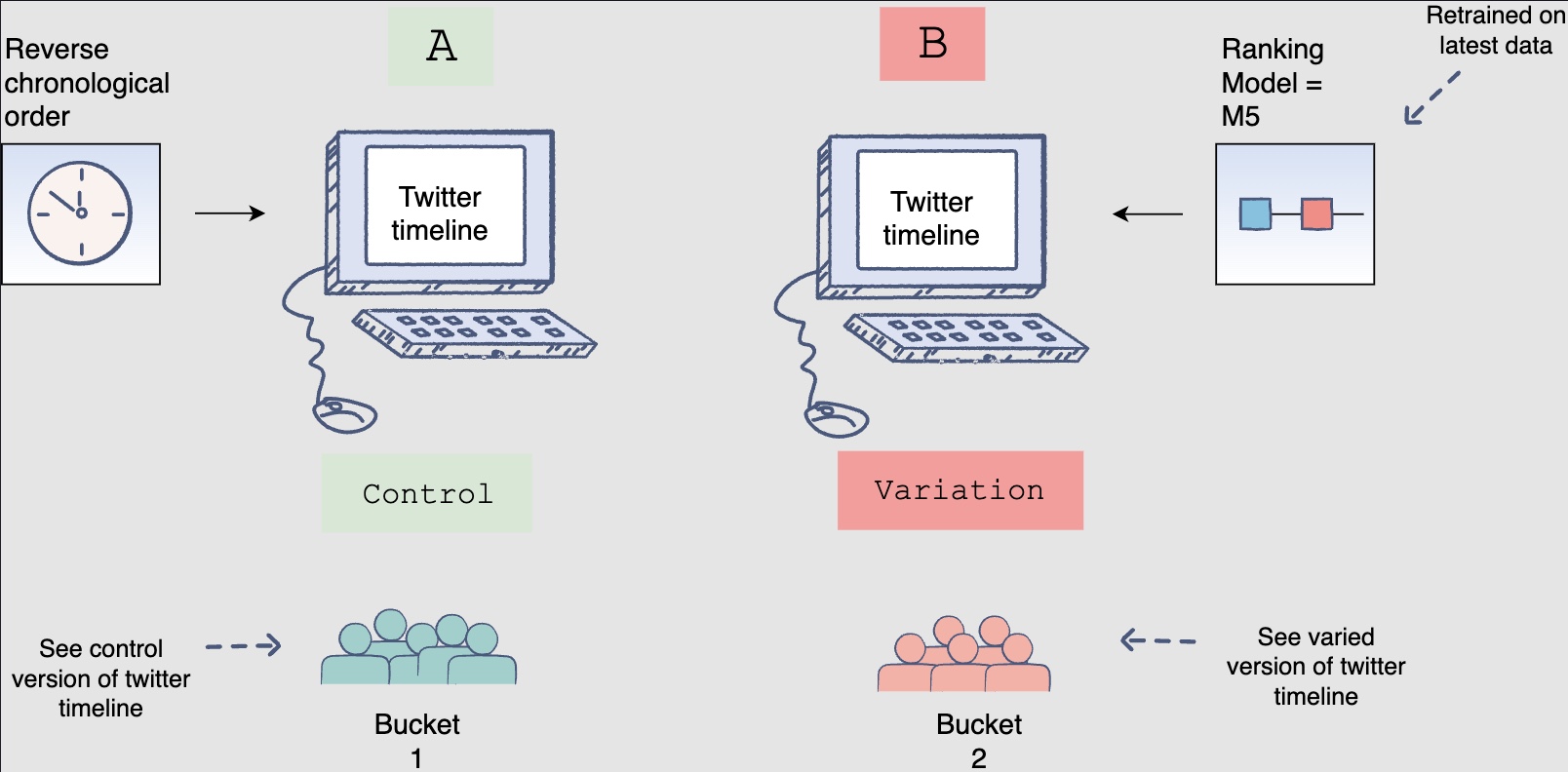
- Now that you have selected the best model offline, you will use A/B testing to compare the performance of this model with the currently deployed model, which displays the feed in reverse chronological order. You will select 1% of the five-hundred million active users, i.e., five million users for the A/B test. Two buckets of these users will be created each having 2.5 million users. Bucket one users will be shown Facebook timelines according to the time-based model; this will be the control group. Bucket two users will be shown the Facebook timeline according to the new ranking model. The following figure shows bucket one users see the control version, whereas Bucket two users see the varied version of the Facebook timeline:
-
However, before you perform this A/B test, you need to retrain the ranking model.
-
Recall that you withheld the most recent partition of the training data to use for validation and testing. This was done to check if the model would be able to predict future engagements on posts given the historical data. However, now that you have performed the validation and testing, you need to retrain the model using the recent partitions of training data so that it captures the most recent phenomena.
Step 4: To deploy or not to deploy
- The results of the A/B tests will help decide whether you should deploy the new ranking model across the platform. The following figure shows engagement aggregates for both buckets of users:
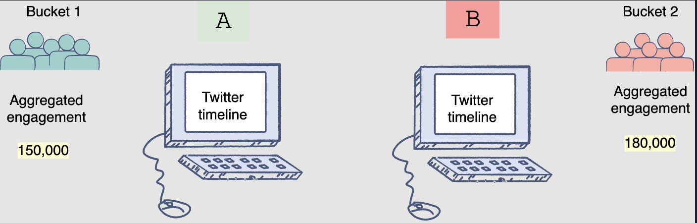
- You can observe that the Facebook feeds generated by the new ranking model had thirty (180k-150k) more engagements.
-
This model is clearly able to outperform the current production, or live state. You should use statistical significance (like p-value) to ensure that the gain is real.
-
Another aspect to consider when deciding to launch the model on production, especially for smaller gains, is the increase in complexity. If the new model increases the complexity of the system significantly without any significant gains, you should not deploy it.
-
To wrap up, if, after an A/B experiment, you see an engagement gain by the model that is statistically significant and worth the complexity it adds to the system, it makes sense to replace the current live system with the new model.
Runtime newsfeed generation
-
Here are issues with running newsfeed generation at runtime:
- We generate the timeline when a user loads their page. This would be quite slow and have a high latency since we have to query multiple tables and perform sorting/merging/ranking on the results.
- Crazy slow for users with a lot of friends/followers as we have to perform sorting/merging/ranking of a huge number of posts.
- For live updates, each status update will result in feed updates for all followers. This could result in high backlogs in our Newsfeed Generation Service.
- For live updates, the server pushing (or notifying about) newer posts to users could lead to very heavy loads, especially for people or pages that have a lot of followers. To improve the efficiency, we can pre-generate the timeline and store it in a memory.
Caching offline generated newsfeeds
-
We can have dedicated servers that are continuously generating users’ newsfeed and storing them in memory for fast processing or in a
UserNewsFeedtable. So, whenever a user requests for the new posts for their feed, we can simply serve it from the pre-generated, stored location. Using this scheme, user’s newsfeed is not compiled on load, but rather on a regular basis and returned to users whenever they request for it. -
Whenever these servers need to generate the feed for a user, they will first query to see what was the last time the feed was generated for that user. Then, new feed data would be generated from that time onwards. We can store this data in a hash table where the “key” would be UserID and “value” would be a STRUCT like this:
Struct {
    LinkedHashMap<FeedItemID, FeedItem> FeedItems;
    DateTime lastGenerated;
}
- We can store
FeedItemIDsin a data structure similar to Linked HashMap or TreeMap, which can allow us to not only jump to any feed item but also iterate through the map easily. Whenever users want to fetch more feed items, they can send the lastFeedItemIDthey currently see in their newsfeed, we can then jump to thatFeedItemIDin our hash-map and return next batch/page of feed items from there.
How many feed items should we store in memory for a user’s feed?
- Initially, we can decide to store 500 feed items per user, but this number can be adjusted later based on the usage pattern.
- For example, if we assume that one page of a user’s feed has 20 posts and most of the users never browse more than ten pages of their feed, we can decide to store only 200 posts per user.
- For any user who wants to see more posts (more than what is stored in memory), we can always query backend servers.
Should we generate (and keep in memory) newsfeeds for all users?
- There will be a lot of users that don’t log-in frequently. Here are a few things we can do to handle this:
- A more straightforward approach could be, to use an LRU based cache that can remove users from memory that haven’t accessed their newsfeed for a long time.
- A smarter solution can be to run ML-based models to predict the login pattern of users to pre-generate their newsfeed, for e.g., at what time of the day a user is active and which days of the week does a user access their newsfeed? etc.
- Let’s now discuss some solutions to our “live updates” problems in the following section.
Model Selection
- We can use a probabilistic sparse linear classifier (logistic regression). This is a popular method because of the computation efficiency that allows it to work well with sparse features.
- With the large volume of data, we need to use distributed training: Logistic Regression in Spark or Alternating Direction Method of Multipliers.
- We can also use deep learning in distributed settings. We can start with the fully connected layers with the Sigmoid activation function applied to the final layer. Because the CTR is usually very small (less than 1%), we would need to resample the training data set to make the data less imbalanced. It’s important to leave the validation set and test set intact to have accurate estimations about model performance.
Evaluation
- One approach is to split the data into training data and validation data.
- Another approach is to replay the evaluation to avoid biased offline evaluation. We use data until time t for training the model. We use test data from time t+1 and reorder their ranking based on our model during inference.
- If there is an accurate click prediction at the correct position, then we record a match. The total match will be considered as total clicks.
- During evaluation we will also evaluate how big our training data set should be, and how frequently we should retrain the model, among many other hyperparameters.
Calculation & estimation#
- Assumptions
- 300 million monthly active users
- On average, a user sees 40 activities per visit. Each user visits 10 times per month.
- We have \(12 * 10^{10}\) or 120 billion observations/samples.
- Data size
- Assume the click through rate is about 1% for 1 month. We collected 1 billion positive labels and about 110 billion negative labels. This is a huge dataset.
- Generally, we can assume that for every data point, we collect hundreds of features. For simplicity, each row takes 500 bytes to store.
- n one month, we need 120 billion rows. Total size \(500^* 120^* 10^9=60^* 10^{12}\) bytes = 60 Terabytes. To save costs we can keep the last 6 months or 1 year of data in the data lake and archive old data in cold storage.
- Scale
- Supports 300 million users
High-level design
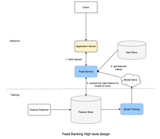
- Feature store is feature values storage. During inference, we need low latency (<10ms) to access features before scoring. Examples of feature stores include MySQL Cluster, Redis, and DynamoDB.
- Item store stores all activities generated by users. It also stores models for the corresponding users. One goal is to maintain the consistent user experience, i.e., to use the same feed ranking method for any particular user. Item store provides the correct model for the corresponding users.
- A user visits the LinkedIn homepage and requests an Application Server for feeds. The Application Server sends feed requests to the Feed Service.
- Feed Service gets the latest model from Model Repos, gets the correct features from the Feature Store, and all the feeds from the ItemStore. Feed Service will provide features for the Model to get predictions.
- The Model returns recommended feeds sorted by click through rate likelihood.
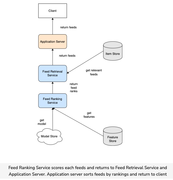
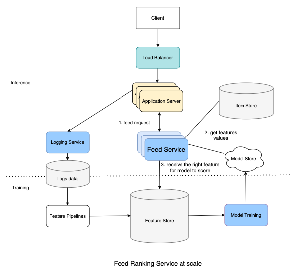
Scale the design
- Scale out the Feed Service module as it represents both Retrieval Service and Ranking Service. This provides better visualization.
- Scale out the Application Server and put the Load Balancer in front of the Application Server to balance load.
Practical Tips
- The approach to follow to ensure success is to touch on all aspects of real day-to-day ML.
- Come with a MVP first by going over data, data privacy, the end product, how are the users going to benefit from the system, what is the baseline, success metrics, what modelling choices do we have, etc.
- Post that, look at more advanced solutions etc. (say, after identifying bottlenecks and suggesting scaling ideas such as load balancing, caching, replication to improve fault tolerance, and data sharding).
Further Reading
- Deep Neural Networks for YouTube Recommendations
- Powered by AI: Instagram’s Explore recommender system
- Google Developers: Recommendation Systems
- Wide & Deep Learning for Recommender Systems
- How TikTok recommends videos #ForYou
- FAISS: A library for efficient similarity search
- Google Developers: Recommendation Systems
- Under the hood: Facebook Marketplace powered by artificial intelligence