Recommendation Systems • Toolkit
- Background
- Embedding Space
- Similarity Measure
- Alternating Least Squares
- Matrix Factorization
- Mean Normalization
- References
Background
- Lately, there’s been a surge in the use of vector-based retrieval methods. These methods work by mapping both users and items into a shared latent vector space, where the inner product of their vectors estimates user-item preferences.
- Well-known techniques such as matrix factorization, factorization machines, and various deep learning approaches fall under this category. Nonetheless, the computational burden can become overwhelming when dealing with vast item sets, as calculating the inner product for each item-user pair is resource-intensive.
- To overcome this, approximate methods like approximate nearest neighbors or maximum inner product search are employed to efficiently pinpoint the most relevant items in large-scale datasets. Among these, tree-based methods, locality-sensitive hashing, product quantization, and navigable small world graphs are prominent for their efficiency.
Embedding Space
- Both the algorithms above, collaborative and content-based filtering, map each document and query to an embedding vector space.
- An embedding is a low-dimensional space into which you can translate high-dimensional vectors. Embeddings make it easier to do machine learning on large inputs like sparse vectors representing words.
- Embeddings are vector representations for an entity. You can represent any discrete entity to a continuous space through Embeddings. Each item in the vector represents a feature or a combination of features for that entity.
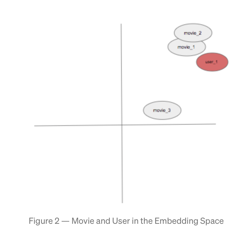
- For example, you can represent movies and user IDs as embeddings. For simplicity, let’s assume that these embeddings are two-dimensional vector as shown in the diagram below. We will create movie and user embeddings and train them along with our neural network.
- The goal is to bring users and movies in a similar embedding space, so we can apply the nearest neighbor based recommendation.
- The figure below shows a hypothetical example where the
user_1is closer tomovie_1andmovie_2in the embedding space than tomovie_3. So we will recommendmovie_1andmovie_2touser_1. - An embedding captures some semantics of the input by placing semantically similar inputs close together in the embedding space. An embedding can be learned and reused across models.
- Similar items (videos, movies) that are watched by the same user, end up closer together in the embedding space. Close here means similarity measure.
- Similar items (videos, movies) that are watched by the same user, end up closer together in the embedding space. Close here means similarity measure.
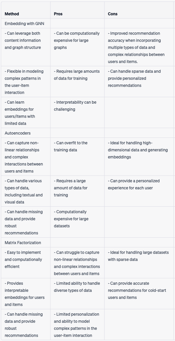
- In terms of recommender systems, there are generally 3 types of embeddings: matrix factorization, autoencoders or graph neural networks (GNN).
Matrix Factorization
- Matrix factorization involves factorizing the user-item interaction matrix into two lower-rank matrices, which can be used to generate embeddings for the users and items.
Autoencoder
- Autoencoders are neural networks that learn to compress and decompress data, and can be used to generate embeddings for users or items by training the network to reconstruct the input data.
GNN
- GNNs are a more recent approach to embedding that leverages graph structures to capture the relationships between items and users. GNNs use message passing algorithms to propagate information across the graph and generate embeddings for the nodes in the graph. This approach is particularly effective for capturing complex dependencies between items and users, as well as for handling heterogeneous types of data.
Similarity Measure
- Similarity measure is a function that takes a pair of embeddings and returns a scalar representing their similarity measure.
- A similarity measure is the squared distance between the two vectors \(\mathbf{v}_{\mathbf{m}}^{(\mathbf{k})}\) and \(\mathbf{v}_{\mathbf{m}}^{(\mathbf{i})}\):
- So why are these embeddings useful and what do we want to glean from them?
- Given a query embedding \(q \subset E\), the model will look for a document \(d \subset E\) such that \(d\) is close to \(q\).
- It will look for embeddings with a larger similarity. In the next section, we will go over methods used to determine “closeness” or “similarity” mathematically in an embedding space.
- Below, we will look at dot-product, cosine, and euclidean distance in more detail but first, we can see how they all compare against each other in the images below. (source)
- The image below shows an example of a query along with three embedding vectors (Item A, Item B, Item C).

- With regard to the three candidates available in the image above, the image below (source) shows how each similarity measure would rank each candidate.

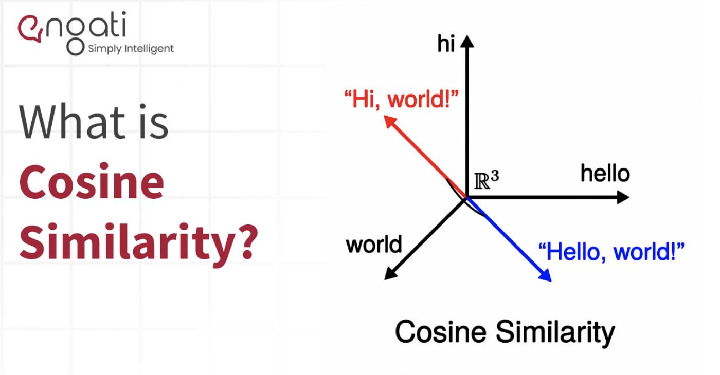
Cosine similarity
- Mathematically, its the measure of the cosine of the angle between two vectors in the embedding space.
Euclidean distance
- This is the distance in Euclidean space, smaller distance meaning higher similarity, larger meaning lower similarity.
Dot Product
- In mathematics, the dot product or scalar product is an algebraic operation that takes two equal-length sequences of numbers (usually coordinate vectors), and returns a single number.
- In Euclidean geometry, the dot product of the Cartesian coordinates of two vectors is widely used. It is often called the inner product (or rarely projection product) of Euclidean space, even though it is not the only inner product that can be defined on Euclidean space (see Inner product space for more).
- Algebraically, the dot product is the sum of the products of the corresponding entries of the two sequences of numbers. Geometrically, it is the product of the Euclidean magnitudes of the two vectors and the cosine of the angle between them. These definitions are equivalent when using Cartesian coordinates.
- In modern geometry, Euclidean spaces are often defined by using vector spaces. In this case, the dot product is used for defining lengths (the length of a vector is the square root of the dot product of the vector by itself) and angles (the cosine of the angle between two vectors is the quotient of their dot product by the product of their lengths).
- The name “dot product” is derived from the centered dot “ · “ that is often used to designate this operation; the alternative name “scalar product” emphasizes that the result is a scalar, rather than a vector, as is the case for the vector product in three-dimensional space.
Alternating Least Squares
- Alternating Least Square is an algorithm used by collaborative filtering to provide accurate predictions to users on items they will enjoy, in an efficient way.
- ALS is an iterative optimization process where we for every iteration try to arrive closer and closer to a factorized representation of our original data.
- It is one kind of collaborative filtering method is used to solve the overfitting issue in sparse data.
- ALS uses matrix factorization, defined below, as a solution to its sparse matrix problem.
- The rating data can be represented as an \(m × n\) matrix. Let’s call this matrix \(R\) where \(n\) is users and \(m\) is items.
- The \((u,i)^{th}\) entry is \(r_{ui}\) in the matrix \(R\) which implies that \((u,i)^{th}\) ratings for \(i^{th}\) item by \(u\) user.
- The \(R\) matrix is sparse matrix as items do not receive ratings from many users. Therefore, the \(R\) matrix has the most missing values.
- A few alternatives to ALS are Singular Value Decomposition and Stochastic Gradient Descent.
- Below is the pseudo code algorithm for ALS:
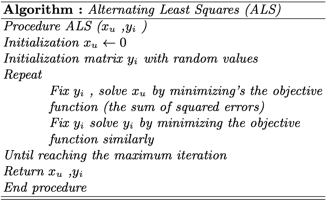
– \(x_{u}\) is \(k\) dimensional vectors summarizing’s every user \(u\). – \(y_{i}\) is \(k\) dimensional vectors summarizing’s every item \(i\).
Matrix Factorization
- We take a large (or potentially huge) matrix and factor it into some smaller representation of the original matrix.
- We end up with two or more, lower dimensional matrices whose product equals the original one.
- When we talk about collaborative filtering for recommender systems we want to solve the problem of our original matrix having millions of different dimensions, but our “tastes” not being nearly as complex.
- Matrix factorization will mathematically reduce the dimensionality of our original “all users by all items” matrix into something much smaller that represents “all items by some taste dimensions” and “all users by some taste dimensions”.
- These dimensions are called latent or hidden features.
- This reduction and working with fewer dimensions makes it both much more efficient and gives us better results.
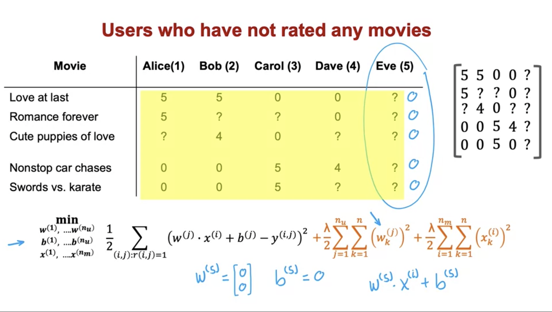
Mean Normalization
- Your algorithm will run more efficiently and perform a bit better on a recommender system if you carry out a mean normalization. This would mean your normalize your ratings to have a consistent value.
- Let’s understand by looking at an example below. Let’s look at Eve, a new user without any ratings, how do we recommend anything to them?
- Lets start by pulling out all the ratings into a matrix:
- Now let’s compute the average for each movie on each row and gather them into a new vector. We will then subtract the mean rating from each of the original ratings.
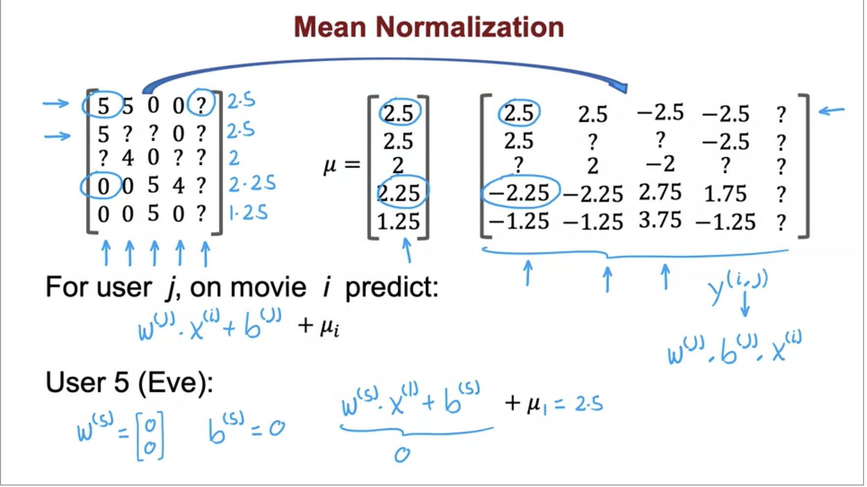
- And this is how we would compute recommendations for Eve!
- Lets start by pulling out all the ratings into a matrix:
References
- Google’s Recommendation Systems Developer Course
- Coursera: Music Recommender System Project
- Coursera: DeepLearning.AI’s specialization.
- Recommender system from learned embeddings
- Google’s Recommendation Systems Developer Crash Course: Embeddings Video Lecture
- ALS introduction by Sophie Wats
- Matrix Factorization
- Recommendation System for E-commerce using Alternating Least Squares (ALS) on Apache Spark