Distilled • Netflix RecSys Design
- Problem statement
- Metrics
- Architectural Components
- Feature Engineering
- Candidate Generation
- Training data generation
- Diversity/Re-ranking
- Online Experimentation
- Runtime newsfeed generation
- Practical Tips
- Further Reading
Problem statement
Metrics
- The feed-ranking system aims to maximize user engagement. So, let’s start by looking at all the user actions on a Facebook feed.
Offline metrics
- During development, we make extensive use of offline metrics (precision (mAP @ k), recall (mAR @ k), F1 score, AUC, log loss, NDCG if precise ranking ground-truth is available from human raters etc.) to guide iterative improvements to our system.
- The purpose of building an offline measurement set is to be able to evaluate our new models quickly. Offline metrics should be able to tell us whether new models will improve the quality of the recommendations or not.
- Can we build an ideal set of items that will allow us to measure recommendation set quality? One way of doing this could be to look at the items that the user has engaged with and see if your recommendation system gets it right using historical data.
- Once we have the set of items that we can confidently say should be on the user’s recommendation list, we can use the following offline metrics to measure the quality of your recommendation system.
mAP @ N
-
One such metric is the Mean Average Precision (mAP @ N) where \(N\) = length of the recommendation list.
-
Let’s go over how this metric is computed so you can build intuition on why it’s good to measure the offline quality.
-
Precision measures the ratio between the relevant recommendations and total recommendations in the movie recommendation list. It will be calculated as follows:
-
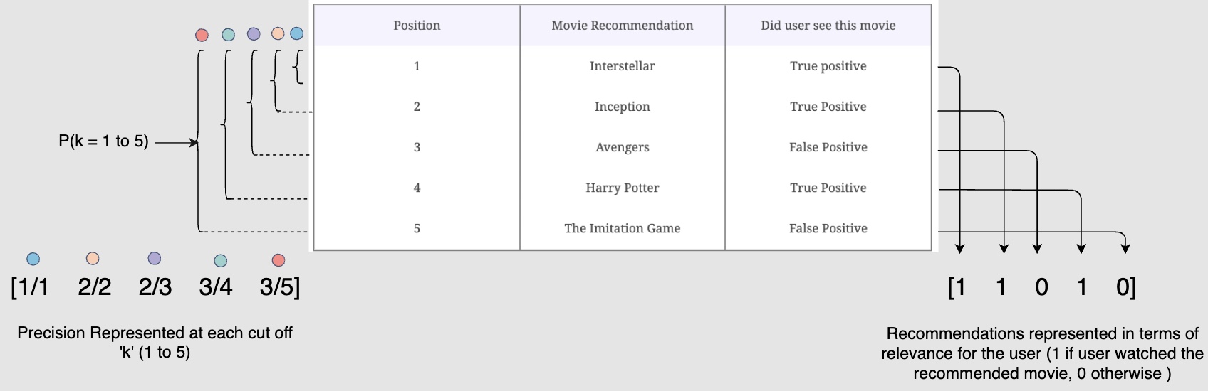
We can observe that precision alone does not reward the early placement of relevant items on the list. However, if we calculate the precision of the subset of recommendations up until each position, k (k = 1 to N), on the list and take their weighted average, we will achieve our goal. Let’s see how.
-
Assume the following:
- The system recommended N = 5 movies.
- The user watched three movies from this recommendation list and ignored the other two.
- Among all the possible movies that the system could have recommended (available on the Netflix platform), only m = 10 are actually relevant to the user (historical data).
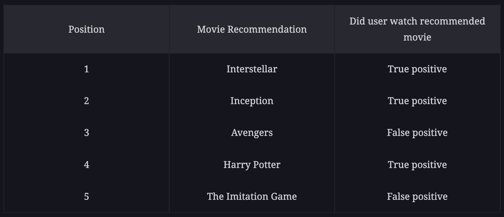
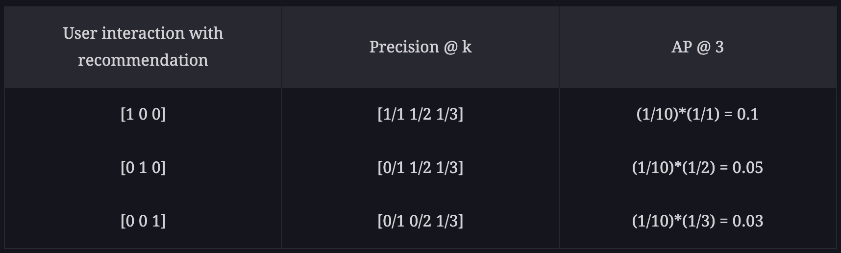
- In the following diagram, we calculate the precision of recommendation subsets up to each position, k, from 1 to 5.
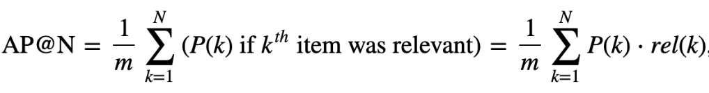
- Now to calculate the average precision (AP), we have the following formula:
-
In the above formula, \(rel(k)\) tells whether that \(k^th\) item is relevant or not.
-
Applying the formula, we have:
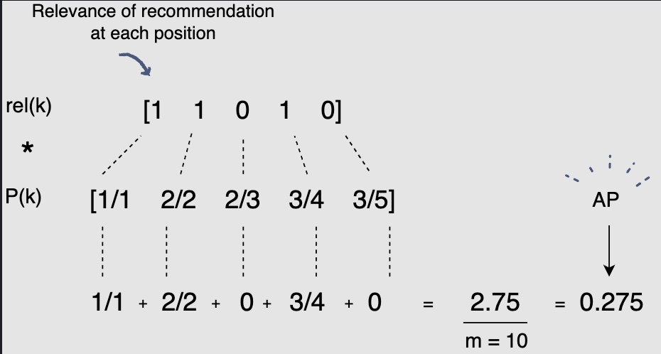
- Here, we see that P(k) only contributes to AP if the recommendation at position k is relevant. Also, observe the “placement legalization” by AP by the following scores of three different recommendation lists:
-
Note that a true positive (1), down the recommendation list, leads to low a mAP compared to the one that is high up in the list. This is important because we want the best recommendations to be at the start of the recommendation set.
-
Lastly, the “mean” in mAP means that we will calculate the AP with respect to each user’s ratings and take their mean. So, mAP computes the metric for a large set of users to see how the system performs overall on a large set.
mAR @ N
-
Another metric that rewards the previously mentioned points is called Mean Average Recall (mAR @ N). It works similar to mAP @ N. The difference lies in the use of recall instead of precision.
-
Recall for your recommendation list is the ratio between the number of relevant recommendations in the list and the number of all possible relevant items(shows/movies). It is calculated as:
-
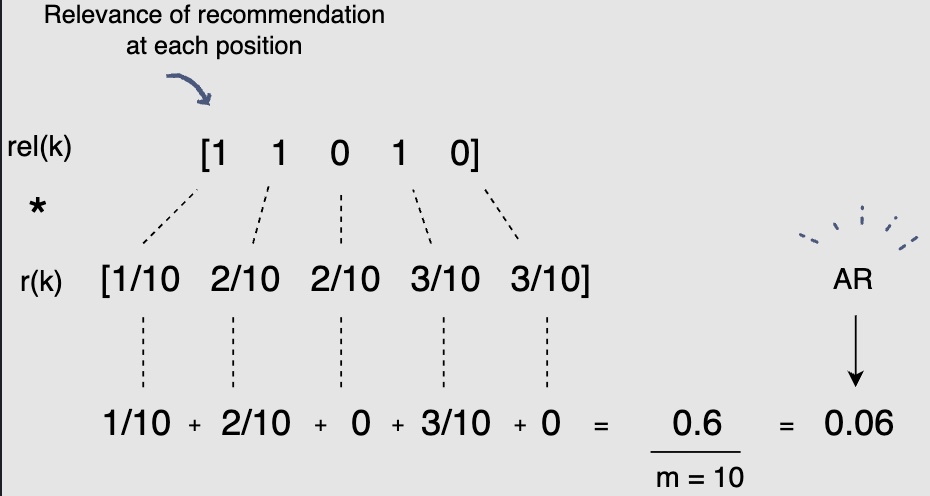
We will use the same recommendation list as used in the mAP @ K example, where N = 5 and m = 10. Let’s calculate the recall of recommendation subsets up to each position, k.
-
The average recall (AR) will then be calculated as follows:
-
Lastly, the “mean” in mAR means that we will calculate AR with respect to each user’s ratings and then take their mean.
-
So, mAR at a high-level, measures how many of the top recommendations (based on historical data) we are able to get in the recommendation set.
F1 score
-
Consider that we have two models, one is giving a better mAP @ N score and the other one was giving a better mAR @ N score. How should you decide which model has better overall performance? If you want to give equal importance to precision and recall, you need to look for a score that conveys the balance between precision and recall.
-
mAP @ N focuses on how relevant the top recommendations are, whereas mAR @ N shows how well the recommender recalls all the items with positive feedback, especially in its top recommendations. You want to consider both of these metrics for the recommender. Hence, you arrive at the final metric “F1 score”.
- So, the F1 score based on mAP and mAR will be a fairly good offline way to measure the quality of your models. Remember that we selected our recommendation set size to be five, but it can be differ based on the recommendation viewport or the number of recommendations that users on the platform generally engage with.
Offline metric for optimizing ratings
- We established above that we optimize the system for implicit feedback data. However, what if the interviewer says that you have to optimize the recommendation system for getting the ratings (explicit feedback) right. Here, it makes sense to use root mean squared error (RMSE) to minimize the error in rating prediction.
- \(\hat{y}^i\) is the recommendation system’s predicted rating for the movie, and \(y_{i}\) is the ground truth rating actually given by the user. The difference between these two values is the error. The average of this error is taken across \(N\) movies.
Online metrics: user engagement/actions
- The following are some options for online metrics that we have for the system. Let’s go over each of them and discuss which one makes the most sense to be used as the key online success indicator.
Engagement rate/CTR
- The success of the recommendation system is directly proportional to the number of recommendations that the user engages with. So, the engagement rate (\frac{sessions with clicks}{total number of sessions}) can help us measure it. However, the user might click on a recommended movie but does not find it interesting enough to complete watching it. Therefore, only measuring the engagement rate with the recommendations provides an incomplete picture.
Videos watched
-
To take into account the unsuccessful clicks on the movie/show recommendations, we can also consider the average number of videos that the user has watched. We should only count videos that the user has spent at least a significant time watching (e.g., more than two minutes).
-
However, this metric can be problematic when it comes to the user starting to watch movie/series recommendations but not finding them interesting enough to finish them.
-
Series generally have several seasons and episodes, so watching one episode and then not continuing is also an indication of the user not finding the content interesting. So, just measuring the average number of videos watched might miss out on overall user satisfaction with the recommended content.
Session watch time
-
Session watch time measures the overall time a user spends watching content based on recommendations in a session. The key measurement aspect here is that the user is able to find a meaningful recommendation in a session such that they spend significant time watching it.
-
To illustrate intuitively on why session watch time is a better metric than engagement rate and videos watched, let’s consider an example of two users, A and B. User A engages with five recommendations, spends ten minutes watching three of them and then ends the session. One the other end, user B engages with two recommendations, spends five minutes on first and then ninety minutes on the second recommendation. Although user A engaged with more content, user B’s session is clearly more successful as they found something interesting to watch.
-
Therefore, measuring session watch time, which is indicative of the session success, is a good metric to track online for the movie recommendation system.
Architectural Components
-
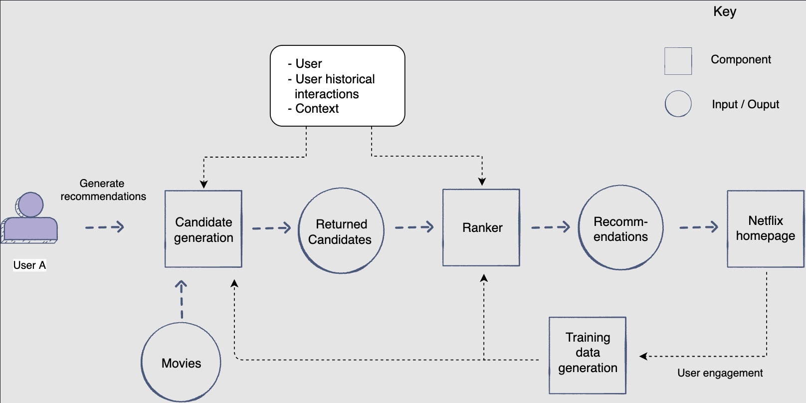
It makes sense to consider generating the best recommendation from a large corpus of movies, as a multi-stage ranking problem. Let’s see why.
-
We have a huge number of movies to choose from. Also, we require complex models to make great, personalized recommendations. However, if we try to run a complex model on the whole corpus, it would be inefficient in terms of execution time and computing resources usage.
-
Therefore, we split the recommendation task into two stages.
- Stage 1: Candidate generation
- Stage 2: Ranking of generated candidates
-
Stage 1 uses a simpler mechanism to sift through the entire corpus for possible recommendations. Stage 2 uses complex strategies only on the candidates given by stage 1 to come up with personalized recommendations.
Candidate Generation/Selection
- Candidate generation is the first step in coming up with recommendations for the user. This component uses several techniques to find out the best candidate movies/shows for a user, given the user’s historical interactions with the media and context.
This component focuses on higher recall, meaning it focuses on gathering movies that might interest the user from all perspectives, e.g., media that is relevant based on historical user interests, trending locally, etc.
Ranker
- The ranker component will score the candidate movies/shows generated by the candidate data generation component according to how interesting they might be for the user.
This component focuses on higher precision, i.e., it will focus on the ranking of the top k recommendations.
- It will ensemble different scores given to a media by multiple candidate generation sources whose scores are not directly comparable. Moreover, it will also use a lot of other dense and sparse features to ensure highly relevant and personalized results.
Feature Engineering
-
To start the feature engineering process, we will first identify the main actors in the movie/show recommendation process:
- The logged-in user
- The media (movie/show)
- The user’s context (e.g., season, time, etc.)
Features
-
Now it’s time to generate features based on these actors. The features would fall into the following categories:
- User-based features
- Context-based features
- Media-based features
- Media-user cross features
User-based features
- Let’s look at various aspects of the user that can serve as useful features for the recommendation model.
age: This feature will allow the model to learn the kind of content that is appropriate for different age groups and recommend media accordingly.gender: The model will learn about gender-based preferences and recommend media accordingly.language: This feature will record the language of the user. It may be used by the model to see if a movie is in the same language that the user speaks.country: This feature will record the country of the user. Users from different geographical regions have different content preferences. This feature can help the model learn geographic preferences and tune recommendations accordingly.average_session_time: This feature (user’s average session time) can tell whether the user likes to watch lengthy or short movies/shows.last_genre_watched: The genre of the last movie that a user has watched may serve as a hint for what they might like to watch next. For example, the model may discover a pattern that a user likes to watch thrillers or romantic movies.
- The following are some user-based features (derived from historical interaction patterns) that have a sparse representation. The model can use these features to figure out user preferences.
user_actor_histogram: This feature would be a vector based on the histogram that shows the historical interaction between the active user and all actors in the media on Netflix. It will record the percentage of media that the user watched with each actor cast in it.user_genre_histogram: This feature would be a vector based on the histogram that shows historical interaction between the active user and all the genres present on Netflix. It will record the percentage of media that the user watched belonging to each genre.user_language_histogram: This feature would be a vector based on the histogram that shows historical interaction between the active user and all the languages in the media on Netflix. It will record the percentage of media in each language that the user watched.
Context-based features:
- Making context-aware recommendations can improve the user’s experience. The following are some features that aim to capture the contextual information.
season_of_the_year: User preferences may be patterned according to the four seasons of the year. This feature will record the season during which a person watched the media. For instance, let’s say a person watched a movie tagged “summertime” (by the Netflix tagger) during the summer season. Therefore, the model can learn that people prefer “summertime” movies during the summer season.upcoming_holiday: This feature will record the upcoming holiday. People tend to watch holiday-themed content as the different holidays approach. For instance, Netflix tweeted that fifty-three people had watched the movie “A Christmas Prince” daily for eighteen days before the Christmas holiday. Holidays will be region-specific as well.days_to_upcoming_holiday: It is useful to see how many days before a holiday the users started watching holiday-themed content. The model can infer how many days before a particular holiday users should be recommended holiday-themed media.time_of_day: A user might watch different content based on the time of the day as well.day_of_week: User watch patterns also tend to vary along the week. For example, it has been observed that users prefer watching shows throughout the week and enjoy movies on the weekend.device: It can be beneficial to observe the device on which the person is viewing content. A potential observation could be that users tend to watch content for shorter periods on their mobile when they are busy. They usually chose to watch on their TV when they have more free time. So, they watch media for a longer period consecutively on their TV. Hence, we can recommend shows with short episodes when a user logs in from their mobile device and longer movies when they log in from their TV.
Media-based features
- We can create a lot of useful features from the media’s metadata.
public-platform-rating: This feature would tell the public’s opinion, such as IMDb/rotten tomatoes rating, on a movie. A movie may launch on Netflix well after its release. Therefore, these ratings can predict how the users will receive the movie after it becomes available on Netflix.revenue: We can also add the revenue generated by a movie before it came to Netflix. This feature also helps the model to figure out the movie’s popularity.time_passed_since_release_date: The feature will tell how much time has elapsed since the movie’s release date.time_on_platform: It is also beneficial to record how long a media has been present on Netflix.media_watch_history: Media’s watch history (number of times the media was watched) can indicate its popularity. Some users might like to stay on top of trends and focus on only watching popular movies. They can be recommended popular media. Others might like less discovered indie movies more. They can be recommended less watched movies that had good implicit feedback (the user watched the whole movie and did not leave it midway). The model can learn these patterns with the help of this feature.
- We can look at the media’s watch history for different time intervals as well. For instance, we can have the following features:
media_watch_history_last_12_hrsmedia_watch_history_last_24_hrs
The media-based features listed above can collectively tell the model that a particular media is a blockbuster, and many people would be interested in watching it. For example, if a movie generates a large revenue, has a good IMDb rating, came to the platform 24 hours ago, and a lot of people have watched it, then it is definitely a blockbuster.
genre: This feature records the primary genre of content, e.g., comedy, action, documentaries, classics, drama, animated, and so on.movie_duration: This feature tells the movie duration. The model may use it in combination with other features to learn that a user may prefer shorter movies due to their busy lifestyle or vice versa.content_set_time_period: This feature describes the time period in which the movie/show was set in. For example, it may show that the user prefers shows that are set in the ’90s.content_tags: Netflix has hired people to watch movies and shows to create extremely detailed, descriptive, and specific tags for the movies/shows that capture the nuances in the content. For instance, media can be tagged as a “Visually-striking nostalgic movie”. These tags greatly help the model understand the taste of different users and find the similarity between the user’s taste and the movies.show_season_number: If the media is a show with multiple seasons, this feature can tell the model whether a user likes shows with fewer seasons or more.country_of_origin: This feature holds the country in which the content was produced.release_country: This feature holds the country where the content was released.release_year: This feature shows the year of theatrical release, original broadcast date or DVD release date.release_type: This feature shows whether the content had a theatrical, broadcast, DVD, or streaming release.maturity_rating: This feature contains the maturity rating of the media with respect to the territory (geographical region). The model may use it along with a user’s age to recommend appropriate movies.
Media-user cross features
- In order to learn the users’ preferences, representing their historical interactions with media as features is very important. For instance, if a user watches a lot of Christopher Nolan movies, that would give us a lot of information about what kind of movies the user likes. Some of these interaction-based features are as follows:
User-genre historical interaction features
- These features represent the percentage of movies that the user watched with the same genre as the movie under consideration. This percentage is calculated for different time intervals to cater to the dynamic nature of user preferences.
user_genre_historical_interaction_3months: The percentage of movies that the user watched with the same genre as the movie under consideration in the last 3 months. For example, if the user watched 6 comedy movies out of the 12 he/she watched in the last 3 months, then the feature value will be: \(\frac{6}{12}=0.5 \text { or } 50 \%\) -This feature shows a more recent trend in the user’s preference for genres as compared to the following feature.user_genre_historical_interaction_1year: This is the same feature as above but calculated for the time interval of one year. It shows a more long term trend in the relationship between the user and genre.user_and_movie_embedding_similarity: Netflix has hired people to watch movies and shows to create incredibly detailed, descriptive, and specific tags for the movies/shows that capture the nuances in the content. For instance, media can be tagged as “Visually-striking nostalgic movie”.- You can have a user embedding based on the tags of movies that the user has interacted with and a media embedding based on its tags. The dot product similarity between these two embeddings can also serve as a feature.
user_actor: This feature tells the percentage of media that the user has watched, which has the same cast (actors) as that of the media under consideration for recommendation.user_director: This feature tells the percentage of movies that the user has watched with the same director as the movie under consideration.user_language_match: This feature matches the user’s language and the media’s language.user_age_match: You will keep a record of the age bracket that has mostly viewed a certain media. This feature will see if the user watching a particular movie/show falls into the same age bracket. For instance, movie A is mostly (80% of the times) watched by people who are 40+. Now, while considering movie A for a recommendation, this feature will see if the user is 40+ or not.
- Some sparse features are described below. Each of them can show popular trends in their respective domains and also the preferences of individual users. We will go over how these sparse features are used in the ranking chapter. You can also go over the embedding chapter about how to generate vector representation of this sparse data to use them in machine learning models.
movie_id: Popular movie IDs are be repeated frequently.title_of_media: This feature holds the title of the movie or the TVV series.synopsis: This feature holds the synopsis or summary of the content.original_title: This feature holds the original title of the movie in its original language. The media may be released for a different country with a different title keeping in view the preference of the nationals. For example, Japanese/Korean movies/shows are released for English speaking countries with English titles as well. -distributor: A particular distributor may be selecting very good quality content, and hence users might prefer content from that distributor. -creator: This feature contains the creator/s of the content. -original_language: This feature holds the original spoken language of the content. If multiple, you can record the choose the majority language. -director: This feature holds the director/s of the content. This feature can indicate directors who are widely popular, such as Steven Spielberg, and it can also showcase the individual preference of users. -first_release_year: This feature holds the year in which content had its first release anywhere (this is different from production year). -music_composer: The music in a show or a film’s score can greatly enhance the storytelling aspect. Users may fancy the work of a particular composer and may be more drawn to their work. -actors: This feature includes the cast of the movie/show.
Candidate Generation
-
The purpose of candidate generation is to select the top k (let’s say one-thousand) movies that you would want to consider showing as recommendations to the end-user. Therefore, the task is to select these movies from a corpus of more than a million available movies.
-
In this lesson, we will be looking at a few techniques to generate media candidates that will match user interests based on the user’s historical interaction with the system.
Candidate generation techniques
- The candidate generation techniques are as follows:
- Collaborative filtering
- Content-based filtering
- Embedding-based similarity
- Each method has its own strengths for selecting good candidates, and we will combine all of them together to generate a complete list before passing it on to the ranked (this will be explained in the ranking lesson).
Training data generation
Train test split
-
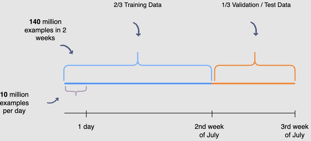
You need to be mindful of the fact that the user engagement patterns may differ throughout the week. Hence, you will use a week’s engagement to capture all the patterns during training data generation. At this rate, you would end up with around seventy million rows of training data.
-
You may randomly select \(\frac{2}{3}^{rd}\) or 66.6% , of the seventy million training data rows that you have generated and utilize them for training purposes. The rest of the \(\frac{1}{3}^{rd}\) or 33.3%, can be used for validation and testing of the model. However, this random splitting defeats the purpose of training the model on an entire week’s data. Also, the data has a time dimension, i.e., we know the engagement on previous posts, and we want to predict the engagement on future posts ahead of time. Therefore, you will train the model on data from one time interval and validate it on the data with the succeeding time interval. This will give a more accurate picture of how the model will perform in a real scenario.
We are building models with the intent to forecast the future.
- In the following illustration, we are training the model using data generated from the first and second week of July and data generated in the thirdweek of July for validation and testing purposes. THe following diagram indicates the splitting data procedure for training, validation, and testing:
- Possible pitfalls seen after deployment where the model is not offering predictions with great accuracy (but performed well on the validation/test splits): Question the data. Garbage in - Garbage out. The model is only as good as the data it was trained on. Data drifts where the real-world data follows a different distribution that the model was trained on are fairly common.
- When was the data acquired? The more recent the data, better the performance of the model.
- Does the data show seasonality? i.e., we need to be mindful of the fact that the user engagement patterns may differ throughout the week. For e.g., don’t use data from weekdays to predict for the weekends.
- Was the data split randomly? Random splitting defeats the purpose since the data has a time dimension, i.e., we know the engagement on previous posts, and we want to predict the engagement on future posts ahead of time. Therefore, you will train the model on data from one time interval and validate it on the data with the succeeding time interval.
Diversity/Re-ranking
- One of the inherent challenges with recommendation engines is that they can inadvertently limit your experience – what is sometimes referred to as a “filter bubble.” By optimizing for personalization and relevance, there is a risk of presenting an increasingly homogenous stream of videos. This is a concern that needs to be addressed when developing our recommendation system.
- Serendipity is important to enable users to explore new interests and content areas that they might be interested in. In isolation, the recommendation system may not know the user is interested in a given item, but the model might still recommend it because similar users are interested in that item (using collaborative filtering).
- Also, another important function of a diversifier/re-ranker is that it boosts the score of fresh content to make sure it gets a chance at propagation. Thus, freshness, diversity, and fairness are the three important areas this block addresses.
- Let’s learn methods to reduce monotony on the user’s Facebook feed.
Why do you need diverse posts?
- Diversity is essential to maintaining a thriving global community, and it brings the many corners of Facebook closer together. To that end, sometimes you may come across a post in your feed that doesn’t appear to be relevant to your expressed interests or have amassed a huge number of likes. This is an important and intentional component of our approach to recommendation: bringing a diversity of posts into your newsfeed gives you additional opportunities to stumble upon new content categories, discover new creators, and experience new perspectives and ideas as you scroll through your feed.
- By offering different videos from time to time, the system is also able to get a better sense of what’s popular among a wider range of audiences to help provide other Facebook users a great experience, too. Our goal is to find balance (exploitation v/s exploration tradeoff) between suggesting content that’s relevant to you while also helping you find content and creators that encourage you to explore experiences you might not otherwise see.
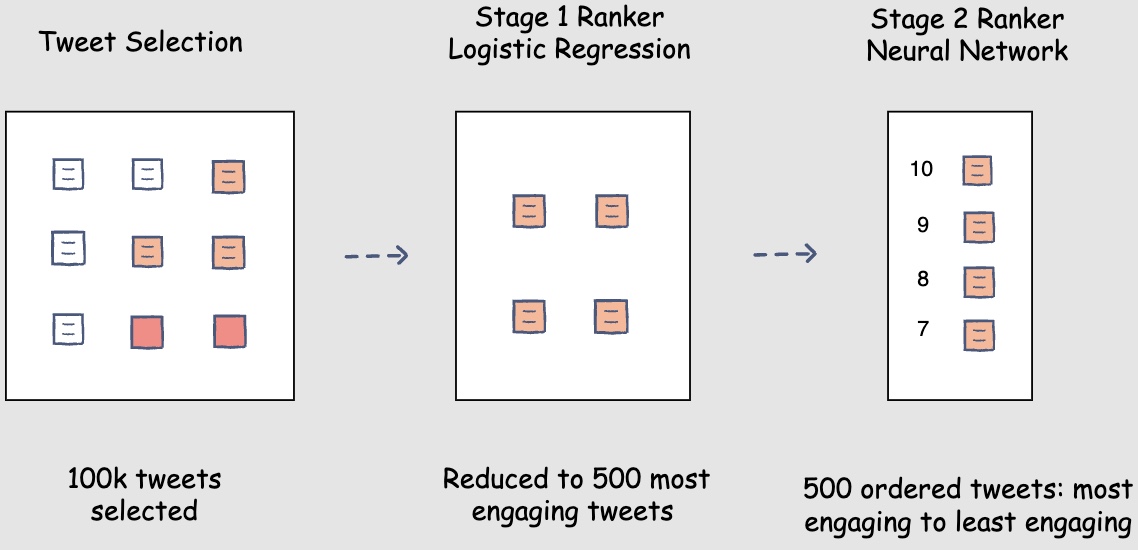
- Let’s assume that you adopted the following modelling option for your Facebook feed ranking system. The post selection component will select one-hundred thousand posts for user A’s Facebook feed. The stage one ranker will choose the top five-hundred most engaging posts for user A. The stage two ranker will then focus on assigning engagement probabilities to these posts with a higher degree of accuracy. Finally, the posts will be sorted according to the engagement probability scores and will be ready for display on the user’s Facebook feed.
-
Consider a scenario where the sorted list of posts has five consecutive posts by the same author. No, your ranking model hasn’t gone bonkers! It has rightfully placed these posts at the top because:
- The logged-in user and the post’s author have frequently interacted with each other’s posts
- The logged-in user and the post’s author have a lot in common like hashtags followed and common followees
- The author is very influential, and their posts generally gain a lot of traction
This scenario remains the same for any modelling option.
Safeguarding the viewing experience
- The newsfeed recommendation system should also be designed with safety as a consideration. Reviewed content found to depict things like graphic medical procedures or legal consumption of regulated goods, for example – which may be shocking if surfaced as a recommended video to a general audience that hasn’t opted in to such content – may not be eligible for recommendation.
- Similarly, videos that have explicitly disliked by the user, have just been uploaded or are under review, and spam content such as videos seeking to artificially increase traffic, also may be ineligible for recommendation into anyone’s newsfeed.
Interrupting repetitive patterns
- To keep your newsfeed interesting and varied, our recommendation system works to intersperse diverse types of content along with those you already know you love. For example, your newsfeed generally won’t show two videos in a row made with the same sound or by the same creator.
- Recommending duplicated content, content you’ve already seen before, or any content that’s considered spam is also not desired. However, you might be recommended a video that’s been well received by other users who share similar interests.
Diversity in posts’ authors
- However, no matter how good of a friend the author is or how interesting their posts might be, user A would eventually get bored of seeing posts from the same author repeatedly. Hence, you need to introduce diversity with regards to the posts’ author.
Diversity in posts’ content
- Another scenario where we might need to introduce diversity is the post’s content. For instance, if your sorted list of posts has four consecutive posts that have videos in them, the user might feel that their feed has too many videos.
Introducing the repetition penalty to interrupt repetitive patterns
-
To rid the Facebook feed from a monotonous and repetitive outlook, we will introduce a repetition penalty for repeated post authors and media content in the post.
-
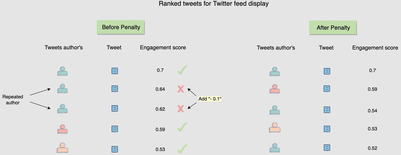
One way to introduce a repetition penalty could be to add a negative weight to the post’s score upon repetition. For instance, in the following diagram, whenever you see the author being repeated, you add a negative weight of -0.1 to the post’s score. The following figure shows a repetition penalty for repeated post author:
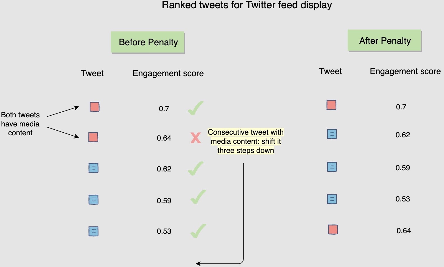
- Another way to achieve the same effect is to bring the post with repetition three steps down in the sorted list. For instance, in the following diagram, when you observe that two consecutive posts have media content in them, you bring the latter down by three steps. The following figure shows a repetition penalty for consecutive posts with media content:
Online Experimentation
-
Let’s see how to evaluate the model’s performance through online experimentation.
-
Let’s look at the steps from training the model to deploying it.
Step 1: Training different models
- Earlier, in the training data generation lesson, we discussed a method of splitting the training data for training and validation purposes. After the split, the training data is utilized to train, say, fifteen different models, each with a different combination of hyperparameters, features, and machine learning algorithms. The following figure shows different models are trained to predict user engagement:
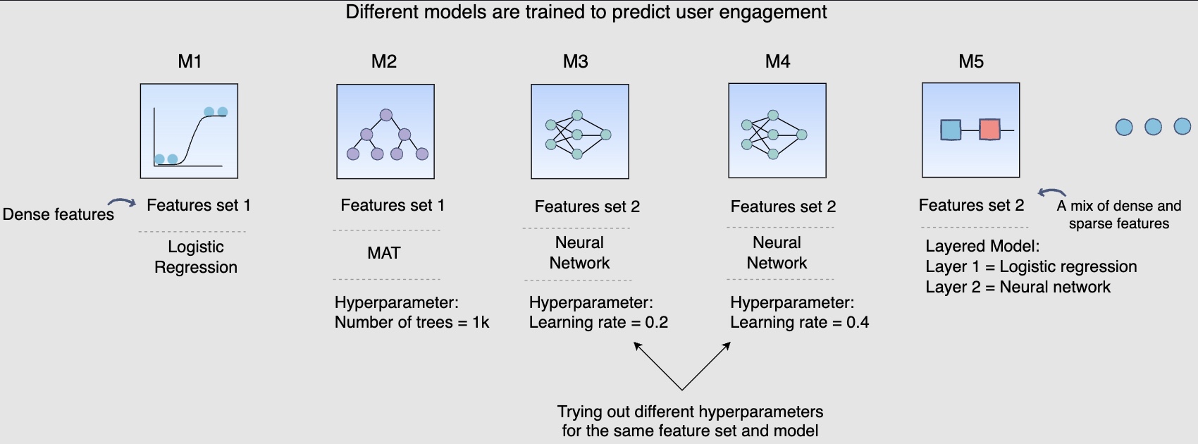
- The above diagram shows different models that you can train for our post engagement prediction problem. Several combinations of feature sets, modeling options, and hyperparameters are tried.
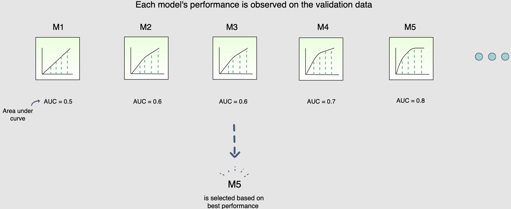
Step 2: Validating models offline
- Once these fifteen models have been trained, you will use the validation data to select the best model offline. The use of unseen validation data will serve as a sanity check for these models. It will allow us to see if these models can generalise well on unseen data. The following figure shows each model’s performance is observed on the validation data
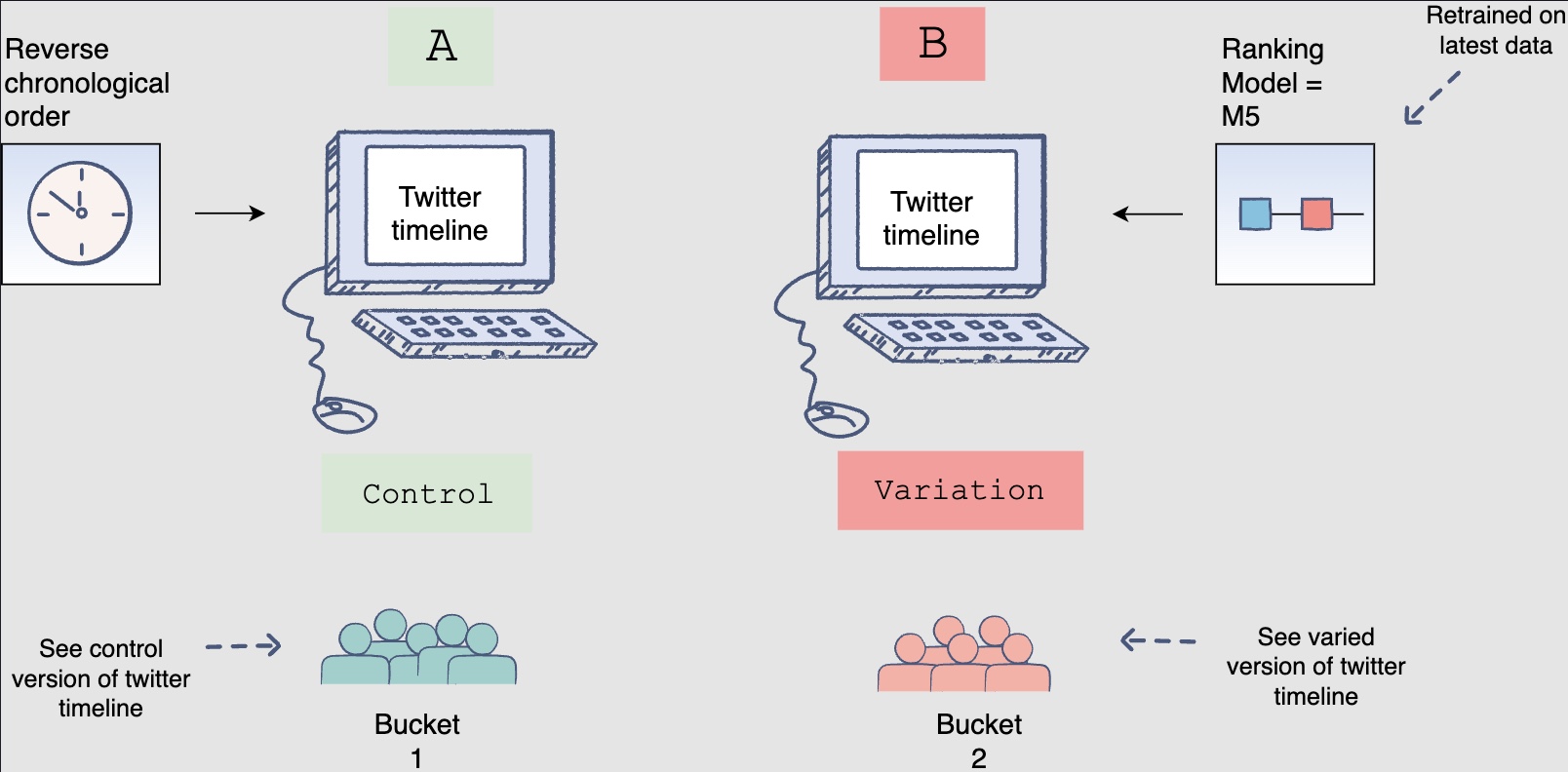
Step 3: Online experimentation
- Now that you have selected the best model offline, you will use A/B testing to compare the performance of this model with the currently deployed model, which displays the feed in reverse chronological order. You will select 1% of the five-hundred million active users, i.e., five million users for the A/B test. Two buckets of these users will be created each having 2.5 million users. Bucket one users will be shown Facebook timelines according to the time-based model; this will be the control group. Bucket two users will be shown the Facebook timeline according to the new ranking model. The following figure shows bucket one users see the control version, whereas Bucket two users see the varied version of the Facebook timeline:
-
However, before you perform this A/B test, you need to retrain the ranking model.
-
Recall that you withheld the most recent partition of the training data to use for validation and testing. This was done to check if the model would be able to predict future engagements on posts given the historical data. However, now that you have performed the validation and testing, you need to retrain the model using the recent partitions of training data so that it captures the most recent phenomena.
Step 4: To deploy or not to deploy
- The results of the A/B tests will help decide whether you should deploy the new ranking model across the platform. The following figure shows engagement aggregates for both buckets of users:
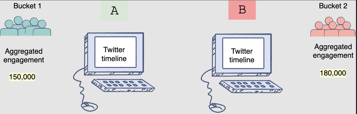
- You can observe that the Facebook feeds generated by the new ranking model had thirty (180k-150k) more engagements.
-
This model is clearly able to outperform the current production, or live state. You should use statistical significance (like p-value) to ensure that the gain is real.
-
Another aspect to consider when deciding to launch the model on production, especially for smaller gains, is the increase in complexity. If the new model increases the complexity of the system significantly without any significant gains, you should not deploy it.
-
To wrap up, if, after an A/B experiment, you see an engagement gain by the model that is statistically significant and worth the complexity it adds to the system, it makes sense to replace the current live system with the new model.
Runtime newsfeed generation
-
Here are issues with running newsfeed generation at runtime:
- We generate the timeline when a user loads their page. This would be quite slow and have a high latency since we have to query multiple tables and perform sorting/merging/ranking on the results.
- Crazy slow for users with a lot of friends/followers as we have to perform sorting/merging/ranking of a huge number of posts.
- For live updates, each status update will result in feed updates for all followers. This could result in high backlogs in our Newsfeed Generation Service.
- For live updates, the server pushing (or notifying about) newer posts to users could lead to very heavy loads, especially for people or pages that have a lot of followers. To improve the efficiency, we can pre-generate the timeline and store it in a memory.
Caching offline generated newsfeeds
-
We can have dedicated servers that are continuously generating users’ newsfeed and storing them in memory for fast processing or in a
UserNewsFeedtable. So, whenever a user requests for the new posts for their feed, we can simply serve it from the pre-generated, stored location. Using this scheme, user’s newsfeed is not compiled on load, but rather on a regular basis and returned to users whenever they request for it. -
Whenever these servers need to generate the feed for a user, they will first query to see what was the last time the feed was generated for that user. Then, new feed data would be generated from that time onwards. We can store this data in a hash table where the “key” would be UserID and “value” would be a STRUCT like this:
Struct {
    LinkedHashMap<FeedItemID, FeedItem> FeedItems;
    DateTime lastGenerated;
}
- We can store
FeedItemIDsin a data structure similar to Linked HashMap or TreeMap, which can allow us to not only jump to any feed item but also iterate through the map easily. Whenever users want to fetch more feed items, they can send the lastFeedItemIDthey currently see in their newsfeed, we can then jump to thatFeedItemIDin our hash-map and return next batch/page of feed items from there.
How many feed items should we store in memory for a user’s feed?
- Initially, we can decide to store 500 feed items per user, but this number can be adjusted later based on the usage pattern.
- For example, if we assume that one page of a user’s feed has 20 posts and most of the users never browse more than ten pages of their feed, we can decide to store only 200 posts per user.
- For any user who wants to see more posts (more than what is stored in memory), we can always query backend servers.
Should we generate (and keep in memory) newsfeeds for all users?
- There will be a lot of users that don’t log-in frequently. Here are a few things we can do to handle this:
- A more straightforward approach could be, to use an LRU based cache that can remove users from memory that haven’t accessed their newsfeed for a long time.
- A smarter solution can be to run ML-based models to predict the login pattern of users to pre-generate their newsfeed, for e.g., at what time of the day a user is active and which days of the week does a user access their newsfeed? etc.
- Let’s now discuss some solutions to our “live updates” problems in the following section.
Practical Tips
- The approach to follow to ensure success is to touch on all aspects of real day-to-day ML. Speak about data, data privacy, the end product, how are the users going to benefit from the system, what is the baseline, success metrics, what modelling choices do we have, can we come with a MVP first and then look at more advanced solutions etc. (say, after identifying bottlenecks and suggesting scaling ideas such as load balancing, caching, replication to improve fault tolerance and data sharding).
Further Reading
- Deep Neural Networks for YouTube Recommendations
- Powered by AI: Instagram’s Explore recommender system
- Google Developers: Recommendation Systems
- Wide & Deep Learning for Recommender Systems
- How TikTok recommends videos #ForYou
- FAISS: A library for efficient similarity search
- Google Developers: Recommendation Systems
- Under the hood: Facebook Marketplace powered by artificial intelligence