Recommendation Systems • Building a Music Recommendation System using PySpark
Code deep-dive
Music recommendation system
- Here, we’re going to have a walk through on building a music recommendation model from scratch.
- This is taken from Music Recommender System Project from Coursera, with a few modifications.
-
We will be specifically using ALS algorithm here for context filtering.
-
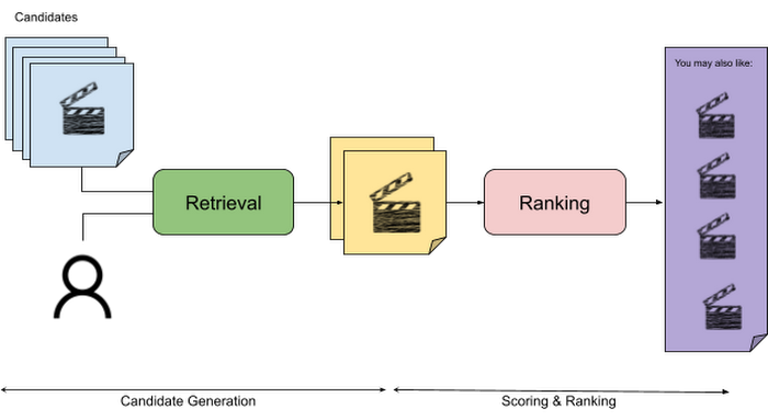
Here is an architectural overview for a movie recommendation system (image credit):
- Let’s get started!
- The code for this whole project is available on my GitHub and the dataset is here.
Step 0) Load up PySpark and start a SparkSession
- Before we begin, run the following code snippet to ensure Google Colab mounts your Google Drive and offers access to it in the Colab environment (if you aren’t using Google Colab, you can simply load the dataset using a URL to the data).
from google.colab import drive drive.mount('/content/drive') - We need to start with importing our data and installing PySpark on our system.
!pip install pyspark - After this, we need to also make sure we import all the required libraries from PySpark for SQL manipulations, creating a SparkSession, and ML libraries for features, and recommendations.
from pyspark.sql import SparkSession from pyspark.sql.functions import count, desc , col, max from pyspark.ml.feature import StringIndexer from pyspark.ml import Pipeline from pyspark.ml.recommendation import ALS from pyspark.ml.tuning import TrainValidationSplit, ParamGridBuilder - Lastly, we also need to create our SparkSession and give our application a name, here we used
lastfm.spark = SparkSession.builder.appName("lastfm").getOrCreate()
Step 1) Load the raw dataset
- First, let’s load up our data set and look at what we’re working with:
file_path = '/content/drive/MyDrive/dataset/dataset/dataset/listenings.csv'
df_listenings = spark.read.format('csv').option('header',True).option('inferSchema',True).load(file_path) #data frame, header will infer column types from csv
df_listenings.show()
+-----------+-------------+--------------------+---------------+--------------------+ | user_id| date| track| artist| album| +-----------+-------------+--------------------+---------------+--------------------+ |000Silenced|1299680100000| Price Tag| Jessie J| Who You Are| |000Silenced|1299679920000|Price Tag (Acoust...| Jessie J| Price Tag| |000Silenced|1299679440000|Be Mine! (Ballad ...| Robyn| Be Mine!| |000Silenced|1299679200000| Acapella| Kelis| Acapella| |000Silenced|1299675660000| I'm Not Invisible| The Tease| I'm Not Invisible| |000Silenced|1297511400000|Bounce (Feat NORE...| MSTRKRFT| Fist of God| |000Silenced|1294498440000|Don't Stop The Mu...| Rihanna|Addicted 2 Bassli...| |000Silenced|1292438340000| ObZen| Meshuggah| ObZen| |000Silenced|1292437740000| Yama's Messengers| Gojira|The Way of All Flesh| |000Silenced|1292436360000|On the Brink of E...| Napalm Death|Time Waits For No...| |000Silenced|1292436360000|On the Brink of E...| Napalm Death|Time Waits For No...| |000Silenced|1292435940000| In Deference| Napalm Death| Smear Campaign| |000Silenced|1292434920000| Post(?)organic| Decapitated|Organic Hallucinosis| |000Silenced|1292434560000| Mind Feeders| Dom & Roland| No Strings Attached| |000Silenced|1292434320000|Necrosadistic War...|Cannibal Corpse| Kill| |000Silenced|1292365560000| Dance All Night| Dom & Roland| Chronology| |000Silenced|1292365260000| Late Night| Dom & Roland| Chronology| |000Silenced|1292365020000| Freak Seen| Dom & Roland| Chronology| |000Silenced|1292364720000|Paradrenasite (Hi...| Dom & Roland| Chronology| |000Silenced|1292364300000| Rhino| Dom & Roland| Chronology| +-----------+-------------+--------------------+---------------+--------------------+ only showing top 20 rows - Here, we are reading our data set from a
.csvformat and inferring the schema, specifically the column types, from this file. - And lastly, we are storing this in our dataframe called
df_listenings.
Step 2) Processing / Data cleanup
- The next step in our code will be to clean up the data and do a bit of data preprocessing before we can train it.
- To make music recommendations, the columns’
user_id,track,artist, and album all seem relevant but date does not, so lets drop it!df_listenings = df_listenings.drop('date') #drops date column df_listenings = df_listenings.na.drop() # removes null values in the row df_listenings.show()+-----------+--------------------+---------------+--------------------+ | user_id| track| artist| album| +-----------+--------------------+---------------+--------------------+ |000Silenced| Price Tag| Jessie J| Who You Are| |000Silenced|Price Tag (Acoust...| Jessie J| Price Tag| |000Silenced|Be Mine! (Ballad ...| Robyn| Be Mine!| |000Silenced| Acapella| Kelis| Acapella| |000Silenced| I'm Not Invisible| The Tease| I'm Not Invisible| |000Silenced|Bounce (Feat NORE...| MSTRKRFT| Fist of God| |000Silenced|Don't Stop The Mu...| Rihanna|Addicted 2 Bassli...| |000Silenced| ObZen| Meshuggah| ObZen| |000Silenced| Yama's Messengers| Gojira|The Way of All Flesh| |000Silenced|On the Brink of E...| Napalm Death|Time Waits For No...| |000Silenced|On the Brink of E...| Napalm Death|Time Waits For No...| |000Silenced| In Deference| Napalm Death| Smear Campaign| |000Silenced| Post(?)organic| Decapitated|Organic Hallucinosis| |000Silenced| Mind Feeders| Dom & Roland| No Strings Attached| |000Silenced|Necrosadistic War...|Cannibal Corpse| Kill| |000Silenced| Dance All Night| Dom & Roland| Chronology| |000Silenced| Late Night| Dom & Roland| Chronology| |000Silenced| Freak Seen| Dom & Roland| Chronology| |000Silenced|Paradrenasite (Hi...| Dom & Roland| Chronology| |000Silenced| Rhino| Dom & Roland| Chronology| +-----------+--------------------+---------------+--------------------+ only showing top 20 rows - Now, we can see that all the null values in the rows are removed and the date column is dropped.
rows = df_listenings.count()
cols = len(df_listenings.columns)
print(rows,cols)
13758905 4 - It seems in total we have over 13 million rows and 4 columns.
Step 3) Aggregation
- In order to make a recommendation model, we first need to know how many times a user has listened to each song, thus understanding their preference.
- We will do this by performing aggregation to see how many times each user has listened to a specific track:
df_listenings_agg = df_listenings.select('user_id', 'track').groupby('user_id', 'track').agg(count('*').alias('count')).orderBy('user_id')
df_listenings_agg.show()
+-------+--------------------+-----+
|user_id|               track|count|
+-------+--------------------+-----+
| --Seph|               Leloo|    1|
| --Seph|         The Embrace|    1|
| --Seph|          Paris 2004|    7|
| --Seph|Chelsea Hotel - L...|    1|
| --Seph|               Julia|    1|
| --Seph|In the Nothing of...|    2|
| --Seph|          I Miss You|    1|
| --Seph| The Riders of Rohan|    1|
| --Seph|Sunset Soon Forgo...|    1|
| --Seph|   Barbados Carnival|    1|
| --Seph|      Fragile Meadow|    1|
| --Seph|          Stupid Kid|    1|
| --Seph|Every Direction I...|    2|
| --Seph|         If It Works|    1|
| --Seph|           So Lonely|    2|
| --Seph|    Kiss with a Fist|    1|
| --Seph|             Starman|    2|
| --Seph|         Left Behind|    2|
| --Seph|   Duel of the Fates|    1|
| --Seph|       Pressure Drop|    1|
+-------+--------------------+-----+
only showing top 20 rows
-
We can see above the track’s and count for the user
Seph.row = df_listenings_agg.count() col = len(df_listenings_agg.columns) print(row,col)- which outputs:
9930128 3
df_listenings_agg = df_listenings_agg.limit(20000)
- If we check our new dataframe with the aggregation,
df_listenings_aggwe can see its a bit over 9 million rows. That’s better than earlier but it’s still a bit too large for our current scope so we add a limit of 20,000 inorder to process faster.
Step 4) Convert the user_id and track columns into unique integers
- We want to use StringIndexer to convert
user_idand track to unique, integer values. - StringIndexer encodes a string column of labels to a column of label indices.
- Note: our dataframe here will be called data for simplicity. Another quick note, our code here deviates from the class’s offerings because we also call
setHandleInvalidtokeep. This is for handling unseen labels during train that are present during test. - To explain the code below a bit, lets look at what each library does:
- A Pipeline chains multiple Transformers and Estimators together to specify an ML workflow. It is specified as a sequence of stages, and each stage is either a Transformer or an Estimator.
- These stages are run in order, and the input DataFrame is transformed as it passes through each stage. For Transformer stages, the
transform()method is called on the DataFrame. - For Estimator stages, the
fit()method is called to produce a Transformer (which becomes part of thePipelineModel, or fitted Pipeline), and that Transformer’stransform()method is called on the DataFrame. - Transformers convert one dataframe into another either by updating the current values of a particular column (like converting categorical columns to numeric) or mapping it to some other values by using a defined logic.
- So in summary, we get back a new dataframe called
datawhich has converted our categorical values into integer ones which is taken from the aggregation we did early. Look atuser_id_indexandtrack_indexbelow to see this in action:
  old_strindexer = [StringIndexer(inputCol = col, outputCol = col + '_index').fit(df_listenings_agg) for col in list(set(df_listenings_agg.columns)- set(['count']))]
  indexer = [curr_strindexer.setHandleInvalid("keep") for curr_strindexer in old_strindexer]
  pipeline = Pipeline(stages = indexer)
  data = pipeline.fit(df_listenings_agg).transform(df_listenings_agg)
  data.show()
- which outputs:
  +-------+--------------------+-----+-------------+-----------+
  |user_id|               track|count|user_id_index|track_index|
  +-------+--------------------+-----+-------------+-----------+
  | --Seph|          Nightmares|    1|         69.0|    10600.0|
  | --Seph|Virus (Luke Fair ...|    1|         69.0|    15893.0|
  | --Seph|Airplanes [feat H...|    1|         69.0|      521.0|
  | --Seph|Belina (Original ...|    1|         69.0|     3280.0|
  | --Seph|              Monday|    1|         69.0|      334.0|
  | --Seph|Hungarian Dance No 5|    1|         69.0|     7555.0|
  | --Seph|       Life On Mars?|    1|         69.0|     1164.0|
  | --Seph|  California Waiting|    1|         69.0|      195.0|
  | --Seph|       Phantom Pt II|    1|         69.0|     1378.0|
  | --Seph|   Summa for Strings|    1|         69.0|    13737.0|
  | --Seph|      Hour for magic|    2|         69.0|     7492.0|
  | --Seph|Hungarian Rhapsod...|    1|         69.0|     7556.0|
  | --Seph|     The Way We Were|    1|         69.0|    14958.0|
  | --Seph| Air on the G String|    1|         69.0|     2456.0|
  | --Seph|Vestido Estampado...|    1|         69.0|    15847.0|
  | --Seph|        Window Blues|    1|         69.0|     1841.0|
  | --Seph| White Winter Hymnal|    3|         69.0|       59.0|
  | --Seph|         The Embrace|    1|         69.0|    14386.0|
  | --Seph|          Paris 2004|    7|         69.0|    11311.0|
  | --Seph|Chelsea Hotel - L...|    1|         69.0|     4183.0|
  +-------+--------------------+-----+-------------+-----------+
  only showing top 20 rows
data = data.select('user_id_index', 'track_index', 'count').orderBy('user_id_index')
data.show()
+-------------+-----------+-----+
|user_id_index|track_index|count|
+-------------+-----------+-----+
|          0.0|    10628.0|    1|
|          0.0|     3338.0|    1|
|          0.0|    12168.0|    1|
|          0.0|    11626.0|    2|
|          0.0|    10094.0|    4|
|          0.0|      427.0|    1|
|          0.0|    16878.0|    1|
|          0.0|    11722.0|    1|
|          0.0|    15074.0|    1|
|          0.0|     1359.0|    1|
|          0.0|     5874.0|    1|
|          0.0|    11184.0|    1|
|          0.0|     2372.0|    2|
|          0.0|    14316.0|    1|
|          0.0|     5346.0|    1|
|          0.0|    11194.0|    1|
|          0.0|     2241.0|    1|
|          0.0|     2864.0|    1|
|          0.0|     2663.0|    4|
|          0.0|     6064.0|    1|
+-------------+-----------+-----+
only showing top 20 rows
Step 5) Train and Test the data
- Let’s finally get to the crux of the matter. Lets split our dataframe 50/50 between training and test
(training, test) = data.randomSplit([0.5,0.5])
- Lets create our model
USERID = "user_id_index"
TRACK = "track_index"
COUNT = "count"

als = ALS(maxIter = 5, regParam = 0.01, userCol = USERID, itemCol = TRACK, ratingCol = COUNT)
# Alternating Least Squares algorithm
model = als.fit(training)
predictions = model.transform(test)
Step 6) Lets get recommending
- Generate top 1- track recommendations for each user.
recs = model.recommendForAllUsers(10)
recs.show()
+-------------+--------------------+
|user_id_index|     recommendations|
+-------------+--------------------+
|            0|[{11940, 44.01194...|
|            1|[{11940, 27.56556...|
|            2|[{11940, 22.33908...|
|            3|[{8819, 18.454283...|
|            4|[{11940, 22.89006...|
|            5|[{11940, 14.14446...|
|            6|[{9321, 6.84029},...|
|            7|[{4460, 13.434702...|
|            8|[{11940, 31.76210...|
|            9|[{11940, 24.63757...|
|           10|[{11940, 42.55469...|
|           11|[{14299, 9.390371...|
|           12|[{11940, 20.56912...|
|           13|[{180, 16.460695}...|
|           14|[{4460, 12.406391...|
|           15|[{8819, 8.37744},...|
|           16|[{14299, 12.00137...|
|           17|[{4460, 10.445208...|
|           18|[{15427, 16.63035...|
|           19|[{3818, 3.9202123...|
+-------------+--------------------+
only showing top 20 rows
- Lastly, lets look at the first element.
recs.take(1)
[Row(user_id_index=0, recommendations=[Row(track_index=11940, rating=44.011940002441406), Row(track_index=8819, rating=11.47814655303955), Row(track_index=2380, rating=5.166903972625732), Row(track_index=102, rating=4.806024551391602), Row(track_index=7134, rating=4.472156047821045), Row(track_index=17139, rating=4.472156047821045), Row(track_index=9550, rating=4.2893452644348145), Row(track_index=2474, rating=4.184332370758057), Row(track_index=1461, rating=3.9852640628814697), Row(track_index=2663, rating=3.9852640628814697)])]
References
- Google’s Recommendation Systems Developer Course
- Coursera: Music Recommender System Project
- Coursera: DeepLearning.AI’s specialization.
- Recommender system from learned embeddings
- Google’s Recommendation Systems Developer Crash Course: Embeddings Video Lecture
- ALS introduction by Sophie Wats
- Matrix Factorization
- Recommendation System for E-commerce using Alternating Least Squares (ALS) on Apache Spark