Distilled • Marketplace RecSys Design
- Problem statement
- Building a product index
- Metrics
- Architectural Components
- Training data generation
- Feature Engineering
- Training Data Generation
- Online Experimentation
- Runtime newsfeed generation
- Extended Features
- Practical Tips
- Further Relistinging
Problem statement
-
Facebook Marketplace was introduced in 2016 as a place for people to buy and sell items within their local communities. Today in the U.S., more than one in three people on Facebook use Marketplace, buying and selling products in categories ranging from cars to shoes to dining tables. Managing the posting and selling of that volume of products with speed and relevance is a daunting task, and the fastest, most scalable way to handle that is to incorporate custom AI solutions.
-
On Marketplace’s second anniversary, we are sharing how we use AI to power it. Whether someone is discovering an item to buy, listing a product to sell, or communicating with a buyer or seller, AI is behind the scenes making the experience better. In addition to the product index and content retrieval systems, which leverage our AI-based computer vision and natural language processing (NLP) platforms, we recently launched some new features that make the process simpler for both buyers and sellers.
-
For buyers, we use computer vision and similarity searches to recommend visually similar products (e.g., suggesting chairs that look similar to the one the buyer is viewing) and the option to have listings translated into their preferred language using machine translation. For sellers, we have tools that simplify the process of creating product listings by autosuggesting the relevant category or pricing, as well as a tool that automatically enhances the lighting in images as they’re being uploaded.
Building a product index
-
Visitors to Marketplace seamlessly interact with these AI-powered features from the moment they arrive to buy or sell something. From the very first search, results are recommended by a content retrieval system coupled with a detailed index that is compiled for every product. Since the only text in many of these listings is a price and a description that can be as brief as “dresser” or “baby stuff,” it was important to build in context from the photos as well as the text for these listings. In practice, we’ve seen a nearly 100 percent increase in consumer engagement with the listings since we rolled out this product indexing system.
-
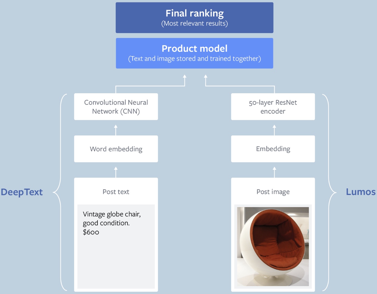
To accomplish this, we built a multimodal ranking system that incorporates Lumos, our image understanding platform, and DeepText, our text understanding engine. As a result, the index for each product includes layers for both the text and the images. To model the word sequence, we map each word from the title and description to an embedding and then feed them into the convolutional neural networks. The image portion comes from a 50-layer ResNet encoder pretrained on the image classification task. The output of the image encoder and the text embedding are concatenated and sent into a multilayer perceptron, where they can be trained and stored together as the complete product model.
Metrics
- The metrics used in our listing prediction system will help select the best machine-learned models to show relevant listings to the user. They should also ensure that these models help the overall improvement of the platform, increase revenue, and provide value for the listing author.
- Like any other optimization problem, there are two types of metrics to measure the effectiveness of our listing prediction system:
- Offline metrics
- Online metrics
Why are both online and offline metrics important? Offline metrics are mainly used to compare the models offline quickly and see which one gives the best result. Online metrics are used to validate the model for an end-to-end system to see how the revenue and engagement rate improve before making the final decision to launch the model.
Offline metrics
- During development, we make extensive use of offline metrics (say, log loss, etc.) to guide iterative improvements to our system.
- The purpose of building an offline measurement set is to be able to evaluate our new models quickly. Offline metrics should be able to tell us whether new models will improve the quality of the recommendations or not.
- Can we build an ideal set of items that will allow us to measure recommendation set quality? One way of doing this could be to look at the items that the user has engaged with and see if your recommendation system gets it right using historical data.
- Once we have the set of items that we can confidently say should be on the user’s recommendation list, we can use the following offline metrics to measure the quality of your recommendation system.
AUC
-
Let’s first go over the area under the receiver operator curve (AUC), which is a commonly used metric for model comparison in binary classification tasks. However, given that the system needs well-calibrated prediction scores, AUC, has the following shortcomings in this listing prediction scenario.
-
AUC does not penalize for “how far off” predicted score is from the actual label. For example, let’s take two positive examples (i.e., with actual label 1) that have the predicted scores of 0.51 and 0.7 at threshold 0.5. These scores will contribute equally to our loss even though one is much closer to our predicted value.
-
AUC is insensitive to well-calibrated probabilities.
-
Log Loss
-
Since, in our case, we need the model’s predicted score to be well-calibrated to use in Auction, we need a calibration-sensitive metric. Log loss should be able to capture this effectively as Log loss (or more precisely cross-entropy loss) is the measure of our predictive error.
-
This metric captures to what degree expected probabilities diverge from class labels. As such, it is an absolute measure of quality, which accounts for generating well-calibrated, probabilistic output.
-
Let’s consider a scenario that differentiates why log loss gives a better output compared to AUC. If we multiply all the predicted scores by a factor of 2 and our average prediction rate is double than the empirical rate, AUC won’t change but log loss will go down.
-
In our case, it’s a binary classification task; a user engages with listing or not. We use a 0 class label for no-engagement (with an listing) and 1 class label for engagement (with an listing). The formula equals:
\[-\frac{1}{N} \sum_{i=1}^{N}\left[y_{i} \log p_{i}+\left(1-y_{i}\right) \log \left(1-p_{i}\right)\right]\]- where:
- \(N\) is the number of observations.
- \(y\) is a binary indicator (0 or 1) of whether the class label is the correct classification for observation.
- \(p\) is the model’s predicted probability that observation is of class (0 or 1).
- where:
Online metrics
- For online systems or experiments, the following are good metrics to track:
Overall revenue
-
This captures the overall revenue generated by the system for the cohorts of the user in either an experiment or, more generally, to measure the overall performance of the system. It’s important to call out that just measuring revenue is a very short term approach, as we may not provide enough value to listing authors and they will move away from the system. However, revenue is definitely one critical metric to track. We will discuss other essential metrics to track shortly.
-
Revenue is basically computed as the sum of the winning bid value (as selected by auction) when the predicted event happens, e.g., if the bid amounts to $0.5 and the user clicks on the listing, the listing author will be charged $0.5. The business won’t be charged if the user doesn’t click on the listing.
Overall listings engagement rate
- Engagement rate measures the overall action rate, which is selected by the listing author.
- Some of the actions might be:
Click rate
- This will measure the ratio of user clicks to listings.
Downstream action rate
- This will measure the action rate of a particular action targeted by the listing author e.g. purchase rate, message rate etc.
- More positive user engagement on the listing results in more revenue:
Counter metrics
-
It’s important to track counter metrics to see if the listings are negatively impacting the platform.
-
We want the users to keep showing engagement with the platform and listings should not hinder that interest. That is why it’s important to measure the impact of listings on the overall platform as well as direct negative feedback provided by users. There is a risk that users can leave the platform if listings degrade the experience significantly.
-
So, for online listings experiments, we should track key platform metrics, e.g., for search engines, is session success going down significantly because of listings? Are the average queries per user impacted? Are the number of returning users on the platform impacted? These are a few important metrics to track to see if there is a significant negative impact on the platform.
-
Along with top metrics, it’s important to track direct negative feedback by the user on the listing such as providing following feedback on the listing:
- Hide listing
- Never see this listing
- Report listing as inappropriate
-
These negative sentiments can lead to the perceived notion of the product as negative.
Architectural Components
- Let’s have a look at the high-level architecture of the system. There will be two main actors involved in our listing prediction system - platform users and listing author. Let’s see how they fit in the architecture:
Listing Generation/Selection
- The listing selection component will fetch the top \(k\) listings based on relevance (subject to the user context).
- To understand the relationship between buyer activity and product content, the system also incorporates a model for the buyer, created with embeddings using the demographic information from the person’s Facebook profile and keywords from searches within Marketplace. The system computes the cosine similarity between the two models as a ranking score, quantifying how closely consumer and product data line up. Using the same models, we are able to use the information gleaned from text, photos, and even logos to proactively detect and remove listings that violate our policies, which allows us to keep the platform safer.
- At this scale, there is a massive product inventory to scan for buyer relevance, so we needed a lightweight computation solution. Using similarity searches reduces the computing load and speeds up the retrieval of relevant products. For these we use Facebook AI similarity search (FAISS), a library for efficient similarity search and clustering of dense vectors.
Listing Ranking/Scoring/Prediction
- After we get the retrieval result, we perform a final ranking using a Sparse Neural Network model with online training. Because the ranking stage model uses more data and more real-time signals (such as the counters of the real-time events that happened on each of the products), it is more accurate — but it’s also computationally heavier, so we do not use it as the model at the retrieval stage; we use it once we’ve already narrowed down the list of all possible items.
- Using more similarity searches and Lumos, Facebook has recently launched another feature to recommend products based on listing images. So if a buyer shows interest in a specific lamp that is no longer available, the system can search the database for similar lamps and promptly recommend several that may be of interest to the buyer.
Training data generation
- We need to record the action taken on an listing. This component takes user action on the listings (displayed after the auction) and generates positive and negative training examples for the listing prediction component.
Funnel model approach
-
For a large scale listings prediction system, it’s important to quickly select an listing for a user based on either the search query and/or user interests. The scale can be large both in terms of the number of listings in the system and the number of users on the platform. So, it’s important to design the system in a way that it can scale well and be extremely performance efficient without compromising on listings quality.
-
To achieve the above objective, it would make sense to use a funnel approach, we gradually move from a large set of listings to a more precise set for the next step in the funnel.
-
Funnel approach: get relevant listings for a user:

-
As we go down the funnel (as shown in the diagram), the complexity of the models becomes higher and the set of listings that they run on becomes smaller. It’s also important to note that the initial layers are mostly responsible for listings selection. On the other hand, listings prediction is responsible for predicting a well-calibrated engagement and quality score for listings. This predicted score is going to be utilized in the auction as well.
-
Let’s go over an example to see how these components will interact for the search scenario.
- A thirty-year old male user issues a query “machine learning”.
- The listings selection component selects all the listings that match the targeting criteria ( user demographics and query) and uses a simple model to predict the listing’s relevance score.
- The listings selection component ranks the listings according to \(r=\text { bid } * \text { relevance }\) and sends the top listings to our listings prediction system.
- The listings prediction component will go over the selected listings and uses a highly optimized ML model to predict a precise calibrated score.
- The listings auction component then runs the auction algorithm based on the bid and predicted listings score to select the top most relevant listings that are shown to the user.
-
We will zoom into the different segments of this diagram as we explore each segment in the upcoming lessons.
Feature Engineering
-
Features are the backbone of any learning system. Let’s think about the main actors or dimensions that will play a key role in our feature engineering process.
- Listing
- Listing author
- User
- Context
-
Now it’s time to generate features based on these actors. The features would fall into the following categories:
- User specific features
- Listing specific features
- Listing author specific features
- Context specific features
- User-listing cross features
- User-listing author cross features
User specific features
user_search_terms: This sparse feature keeps a record of the user’s search query terms.user_previous_search_terms: This sparse feature specifies what users have searched in the past. This helps in recommending listings based on past user preferences.user_interests: This sparse feature specifies the interests listed on their profile. This helps in recommending listings based on the user’s interests.region: This feature records the country of the user. Users from different geographical regions have different content preferences. This feature can help the model learn regional preferences and tune the recommendations accordingly.age: This feature records the age of the user. It allows the model to learn the kind of listing that is appropriate according to different age groups.gender: The model learns about gender-based preferences.language: This feature records the language of the user.embedding_last_k_listings: The model will learn about the interest of the user using the history of the user’s activity on the last k listings that were shown. We can make one embedding by combining embedding vectors of the last k listings that the user engaged with.- Embedding of user’s last watched listings:
engagement_content_type: This takes into account the content of the listing that the user engages with. Here, we can track which type of listing a user plays around with, such as a video or an image listing.engagement_days: This feature captures the user activity on each day of the week. For example, the user might be more active on weekends rather than on weekdays.platform_time_spent: This feature captures how long the user has been on the platform. This can be useful because we can show a different listing set to the user every hour to maximize their engagement with the listing.
Listing specific features
listing_id: A unique id is assigned to each listing and can be used as a sparse feature. Utilizing listing_id as a sparse feature allows the model to memorize historical engagement for each listing, and it can also be used in interesting cross features for memorization (such as listing_id * user interests). listingditionally, we can also generate embeddings during training time for the listing using its id, as we will discuss in the listing prediction section.listing_content_raw_terms: listing terms can also be very useful sparse features. They can tell us a lot about the listing, e.g., a good model can learn from the text’s content to identify what the listing is about, such as politics or sports. Raw terms allow the models (especially NN models) to learn such behavior from given raw terms.historical_engagement_rate: This feature specifies the rate of user engagement with the listing. Here we will measure engagement in different windows such as different times of the day or days of the week. For instance, we can have the following features:listing_engagement_history_last_24_hrs: Since listings are short-lived, recent engagement is important. This feature captures the most recent engagement with the listing.listing_engagement_history_last_7_days: This captures the activity on the listing on each day of the week. For example, an listing can get more engagement on weekends rather than on weekdays.
This feature can tell the model that a particular listing is performing well. This prior engagement data can help predict future engagement behavior.
listing_impressions: This feature records the number of times an listing is viewed. This is helpful since we can train the model on the engagement rate as a feature when we have a reasonable number of listing impressions. We can select the cut-off point until which we want to consider the impressions. For example, we can say that if a particular listing has twenty impressions, we can measure the historical engagement rate.listing_negative_engagement_rate: This feature keeps a record of negative engagement (hide, report) with the listing.listing_embedding: We can generate embedding for an listing given all the data that we know about it e.g. listing terms and engagement data. This embedding is then a dense representation of the listing that can be used in modeling. Please refer to our embedding lesson to see how we can generate this embedding.- listing embedding can also be used to detect the listing’s category, e.g., it can tell if the listing belongs to sports, etc.
- Detect the category/group from the given listing embedding
listing_age: This feature specifies how old the listing is.
Listing author specific features
listing_author_domain: This is a sparse feature that keeps a record of the areas that a listing author lists in. This can be used in the same way for memorization and embedding generation as discussed for listing_id.historical_engagement_rate: This feature specifies the ratio of user engagement with listings posted by a particular listing author.region_wise_engagement: The system should learn to show listings specific to a region from the histogram of engagement based on region. From an listing author’s perspective, the listing posted by an listing author can be restricted to a specific region based on the listing content.- For example, an American football listing posted by the listing author will be most relevant to people living in the United States. This relevance can be predicted using the given histogram of engagement between the users and the listing.
- Histogram to show user’s engagement region-wise with the listing:
Context specific features
current_region: This feature keeps track of the geographical location of the user. Note that the context may change if the user travels to other parts of the world. The system should learn the context of the user and show listings accordingly.time: This feature will show listings subject to time of the day. The user would be able to see a different set of listings appear throughout the day.deviceorscreen_size: It can be beneficial to observe the device a person is using to view content on. A potential observation could be that a user tends to watch content for shorter bursts on their mobile. However, they he usually chooses to watch on their laptop when they have more free time, so they watch for longer periods consecutively. The size of the screen is an important feature because if the users are using a device with a small screen size, there is a possibility that listings are actually never seen by the users. This is because they don’t scroll far down enough to bring the listings in-view.
User-listing cross features
embedding_similarity: Here, we can generate vectors for the user’s interest and the listing’s content. We can generate embedding vectors for listings based on their content and for the user based on their interactions with the listing. A dot product between these vectors can be calculated to measure their similarity. A high score would equate to a highly relevant listing for the user. Please refer to our embedding lesson to see a few methods for generating these embeddings.- For example, the listing is about tennis and the user is not interested in tennis. Therefore, this feature will have a low similarity score.
- User-listing embedding based similarity as a feature for the model:
region_wise_engagement: An listing engagement radius can be another important feature. For example, the listing-user histogram below shows that an American Football listing is mostly viewed by people living in America.- Histogram to show user’s engagement region-wise with the listing:
user_listing_category_histogram: This feature observes user engagement on an listing category using a histogram plot showing user engagement on an listing category.- The following histogram shows that user engagement is the highest on the sports listing:
user_listing_subcategory_histogram: This feature observes user engagement on an listing subcategory using a histogram plot that shows user engagement on an listing subcategory.- The following histogram shows that user engagement is the highest on the football listing:
user_gender_listing_histogram: Some listings can be more appealing to a specific gender. This similarity can be calculated by making a histogram plot showing user engagement gender-wise on an listing. For example, if the listing is for female clothing, it may be primarily of interest to women.- User_gender-listing histogram based on historical interaction:
user_age_listing_histogram: Auser_agehistogram can be used to predict user age-wise engagement.- User-listing_age histogram based on historical interaction:
User-listing author cross features
embedding_similarity: We can project the listing author and user in the same embedding space to see how close they are. From the embedding similarity score, we can figure out the type of listings the listing author shows, and whether the user clicks on those types of listings.- User-listing author embedding based similarity as a feature for the model:
user_gender_listing_author_histogram: This feature observes gender-wise user engagement on an listing posted by an listing author using a histogram plot. For example, the listing author’s listing for male clothing might be more engaging for men than women.- User_gender-listing author histogram based on historical interaction:
user_age_listing_author_histogram: This feature observes age-wise user engagement on an listing posted by an listing author using a histogram plot.- For example, a young audience might demonstrate a greater inclination towards the listing author’s listing on pop music.
- User_age-listing author histogram based on historical interaction:
Training Data Generation
- The performance of the user engagement prediction model will depend drastically on the quality and quantity of training data. So let’s see how the training data for our model can be generated.
Training data generation through online user engagement
-
When we show an listing to the user, they can engage with it or ignore it. Positive examples result from users engaging with listings, e.g., clicking or listingding an item to their cart. Negative examples result from users ignoring the listings or providing negative feedback on the listing.
-
Suppose the listing author specifies “click” to be counted as a positive action on the listing. In this scenario, a user-click on an listing is considered as a positive training example, and a user ignoring the listing is considered as a negative example.
-
Click counts as positive example:
- Suppose the listing refers to an online shopping platform and the listing author specifies the action “listingd to cart” to be counted as positive user engagement. Here, if the user clicks to view the listing and does not listingd items to the cart, it is counted as a negative training example.
- “listingd to cart” counts as a positive training example:
Balancing positive and negative training examples
-
Users’ engagement with an listing can be fairly low based on the platform e.g. in case of a feed system where people generally browse content and engage with minimal content, it can be as low as 2-3%.
-
How would this percentage affect the ratio of positive and negative examples on a larger scale?
-
Let’s look at an extreme example by assuming that one-hundred million listings are viewed collectively by the users in a day with a 2% engagement rate. This will result in roughly two million positive examples (where people engage with the listing) and 98 million negative examples (where people ignore the listing).
-
In order to balance the ratio of positive and negative training samples, we can randomly down sample the negative examples so that we have a similar number of positive and negative examples.
Model recalibration
- Negative downsampling can accelerate training while enabling us to learn from both positive and negative examples. However, our predicted model output will now be in the downsampling space. For instance, consider that if our engagement rate is 5% and we select only 10% negative samples, our average predicted engagement rate will be near 50%.
-
Auction uses this predicted rate to determine order and pricing; therefore it’s critical that we recalibrate our score before sending them to auction. The recalibration can be done using:
\[q=\frac{p}{p+(1-p) / w}\] - where,
- \(q\) is the re-calibrated prediction score,
- \(p\) is the prediction in downsampling space, and
- \(w\) is the negative downsampling rate.
Train test split
-
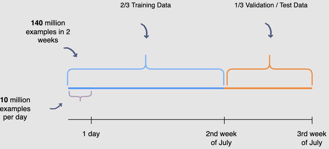
You need to be mindful of the fact that the user engagement patterns may differ throughout the week. Hence, you will use a week’s engagement to capture all the patterns during training data generation. At this rate, you would end up with around seventy million rows of training data.
-
You may randomly select \(\frac{2}{3}^{rd}\) or 66.6% , of the seventy million training data rows that you have generated and utilize them for training purposes. The rest of the \(\frac{1}{3}^{rd}\) or 33.3%, can be used for validation and testing of the model. However, this random splitting defeats the purpose of training the model on an entire week’s data. Also, the data has a time dimension, i.e., we know the engagement on previous posts, and we want to predict the engagement on future posts ahelisting of time. Therefore, you will train the model on data from one time interval and validate it on the data with the succeeding time interval. This will give a more accurate picture of how the model will perform in a real scenario.
We are building models with the intent to forecast the future.
- In the following illustration, we are training the model using data generated from the first and second week of July and data generated in the thirdweek of July for validation and testing purposes. THe following diagram indicates the splitting data procedure for training, validation, and testing:
- Possible pitfalls seen after deployment where the model is not offering predictions with great accuracy (but performed well on the validation/test splits): Question the data. Garbage in - Garbage out. The model is only as good as the data it was trained on. Data drifts where the real-world data follows a different distribution that the model was trained on are fairly common.
- When was the data acquired? The more recent the data, better the performance of the model.
- Does the data show seasonality? i.e., we need to be mindful of the fact that the user engagement patterns may differ throughout the week. For e.g., don’t use data from weekdays to predict for the weekends.
- Was the data split randomly? Random splitting defeats the purpose since the data has a time dimension, i.e., we know the engagement on previous posts, and we want to predict the engagement on future posts ahelisting of time. Therefore, you will train the model on data from one time interval and validate it on the data with the succeeding time interval.
Online Experimentation
-
Let’s see how to evaluate the model’s performance through online experimentation.
-
Let’s look at the steps from training the model to deploying it.
Step 1: Training different models
- Earlier, in the training data generation lesson, we discussed a method of splitting the training data for training and validation purposes. After the split, the training data is utilized to train, say, fifteen different models, each with a different combination of hyperparameters, features, and machine learning algorithms. The following figure shows different models are trained to predict user engagement:

- The above diagram shows different models that you can train for our post engagement prediction problem. Several combinations of feature sets, modeling options, and hyperparameters are tried.
Step 2: Validating models offline
- Once these fifteen models have been trained, you will use the validation data to select the best model offline. The use of unseen validation data will serve as a sanity check for these models. It will allow us to see if these models can generalise well on unseen data. The following figure shows each model’s performance is observed on the validation data

Step 3: Online experimentation
- Now that you have selected the best model offline, you will use A/B testing to compare the performance of this model with the currently deployed model, which displays the feed in reverse chronological order. You will select 1% of the five-hundred million active users, i.e., five million users for the A/B test. Two buckets of these users will be created each having 2.5 million users. Bucket one users will be shown Facebook timelines according to the time-based model; this will be the control group. Bucket two users will be shown the Facebook timeline according to the new ranking model. The following figure shows bucket one users see the control version, whereas Bucket two users see the varied version of the Facebook timeline:

-
However, before you perform this A/B test, you need to retrain the ranking model.
-
Recall that you withheld the most recent partition of the training data to use for validation and testing. This was done to check if the model would be able to predict future engagements on posts given the historical data. However, now that you have performed the validation and testing, you need to retrain the model using the recent partitions of training data so that it captures the most recent phenomena.
Step 4: To deploy or not to deploy
- The results of the A/B tests will help decide whether you should deploy the new ranking model across the platform. The following figure shows engagement aggregates for both buckets of users:

- You can observe that the Facebook feeds generated by the new ranking model hlisting thirty (180k-150k) more engagements.
-
This model is clearly able to outperform the current production, or live state. You should use statistical significance (like p-value) to ensure that the gain is real.
-
Another aspect to consider when deciding to launch the model on production, especially for smaller gains, is the increase in complexity. If the new model increases the complexity of the system significantly without any significant gains, you should not deploy it.
-
To wrap up, if, after an A/B experiment, you see an engagement gain by the model that is statistically significant and worth the complexity it listingds to the system, it makes sense to replace the current live system with the new model.
Runtime newsfeed generation
-
Here are issues with running newsfeed generation at runtime:
- We generate the timeline when a user lolistings their page. This would be quite slow and have a high latency since we have to query multiple tables and perform sorting/merging/ranking on the results.
- Crazy slow for users with a lot of friends/followers as we have to perform sorting/merging/ranking of a huge number of posts.
- For live updates, each status update will result in feed updates for all followers. This could result in high backlogs in our Newsfeed Generation Service.
- For live updates, the server pushing (or notifying about) newer posts to users could lelisting to very heavy lolistings, especially for people or pages that have a lot of followers. To improve the efficiency, we can pre-generate the timeline and store it in a memory.
Caching offline generated newsfeeds
-
We can have dedicated servers that are continuously generating users’ newsfeed and storing them in memory for fast processing or in a
UserNewsFeedtable. So, whenever a user requests for the new posts for their feed, we can simply serve it from the pre-generated, stored location. Using this scheme, user’s newsfeed is not compiled on lolisting, but rather on a regular basis and returned to users whenever they request for it. -
Whenever these servers need to generate the feed for a user, they will first query to see what was the last time the feed was generated for that user. Then, new feed data would be generated from that time onwards. We can store this data in a hash table where the “key” would be UserID and “value” would be a STRUCT like this:
Struct {
    LinkedHashMap<FeedItemID, FeedItem> FeedItems;
    DateTime lastGenerated;
}
- We can store
FeedItemIDsin a data structure similar to Linked HashMap or TreeMap, which can allow us to not only jump to any feed item but also iterate through the map easily. Whenever users want to fetch more feed items, they can send the lastFeedItemIDthey currently see in their newsfeed, we can then jump to thatFeedItemIDin our hash-map and return next batch/page of feed items from there.
How many feed items should we store in memory for a user’s feed?
- Initially, we can decide to store 500 feed items per user, but this number can be listingjusted later based on the usage pattern.
- For example, if we assume that one page of a user’s feed has 20 posts and most of the users never browse more than ten pages of their feed, we can decide to store only 200 posts per user.
- For any user who wants to see more posts (more than what is stored in memory), we can always query backend servers.
Should we generate (and keep in memory) newsfeeds for all users?
- There will be a lot of users that don’t log-in frequently. Here are a few things we can do to handle this:
- A more straightforward approach could be, to use an LRU based cache that can remove users from memory that haven’t accessed their newsfeed for a long time.
- A smarter solution can be to run ML-based models to predict the login pattern of users to pre-generate their newsfeed, for e.g., at what time of the day a user is active and which days of the week does a user access their newsfeed? etc.
- Let’s now discuss some solutions to our “live updates” problems in the following section.
Extended Features
Enriching buyer and seller interactions by suggesting message responses
- Messenger allows buyers and sellers to communicate about a product directly. When chatting in Messenger, M, an automated assistant powered by AI, makes suggestions to help people communicate and get things done. For example, in a 1:1 conversation, when a seller is asked a question such as “Is the bicycle still available?” M can suggest replies like “Yes,” “No,” or “I think so.”
Missed an item? Let Facebook find you similar ones
- If the answer is no, the product is no longer available, then M may prompt the buyer with a suggestion to “Find more like this on Marketplace” with a link to a page of items similar to the one the buyer was asking about. This list is compiled using our similarity search functionality.
Message language detection and translation
-
If M detects that a person received a message in a language that is different from his or her default language, it will offer to translate this message. Messages are translated using our neural machine translation platform, the same technology that translates posts and comments on Facebook and Instagram.
-
All these suggestions are automatically generated by an AI system that was trained via machine learning to recognize intent. We use different neural net models to determine the intent and whether to show a suggestion. We also use entity extractors like Duckling to identify things like dates, times, and locations. For some suggestions, we use additional neural net models to rank different suggestions to ensure the most relevant options are surfaced (like translation, stickers, or replies). M also learns and becomes more personalized over time, so if you interact with one suggestion more regularity, M might surface it more. If you use another less (or not at all), M will adapt accordingly. This entire process is automated and powered by artificial intelligence.
Practical Tips
- The approach to follow to ensure success is to touch on all aspects of real day-to-day ML. Speak about data, data privacy, the end product, how are the users going to benefit from the system, what is the baseline, success metrics, what modelling choices do we have, can we come with a MVP first and then look at more listingvanced solutions etc. (say, after identifying bottlenecks and suggesting scaling ideas such as lolisting balancing, caching, replication to improve fault tolerance and data sharding).
Further Relistinging
- Deep Neural Networks for YouTube Recommendations
- Powered by AI: Instagram’s Explore recommender system
- Google Developers: Recommendation Systems
- Wide & Deep Learning for Recommender Systems
- How TikTok recommends videos #ForYou
- FAISS: A library for efficient similarity search
- M Now Offers Suggestions to Make Your Messenger Experience More Useful, Seamless and Delightful
- Google Developers: Recommendation Systems
- Under the hood: Facebook Marketplace powered by artificial intelligence