Recsys - Embeddings
- Overview
- Factorization Machines (FM) vs. Matrix Factorization (MF)
- Representing Demographic Data
- Content-Based Filtering
- Comparative Analysis
- FAQ
- How are sparse/one-hot vectors embedded as continuous embeddings to the input of a neural recommender system?
- How do you embed IDs (particularly when they can be in the billions) as part of the input features for a recommender system?
- How do you (re-)initialize an Embedding Layer as new IDs (users or items) being added?
- Expand on the Hashing Trick. Give examples of various hashes that typical recommender systems use.
- Why are neural recommender architectures (such as neural collaborative filtering) better than their traditional counterparts for handling sparsity?
- Conclusion
- How are Factorization Machines different from Deep Factorization Machines?
- In the context of recommender systems, are neural networks or traditional ML techniques better at handling sparsity?
- Can traditional ML algorithms (such as logistic regression) take as input both sparse and dense features?
Overview
- This article will go over different methods of generating embeddings in recommender systems.
- Embeddings are a key component in many recommender systems. They provide low-dimensional vector representations of users and items that capture latent characteristics. Here are some common embedding techniques used in recommenders:
Neural Collaborative Filtering (NCF)
- Input: User-item interaction data (e.g., ratings, clicks).
- Computation: Trains a neural network model on the interaction data to learn embeddings for users and items that can predict interactions. Combines matrix factorization and multi-layer perceptron approaches.
- Output: Learned user and item embeddings.
- Advantages: Captures complex non-linear patterns. Performs well on sparse data.
- Limitations: Requires large amounts of training data. Computationally expensive.
Matrix Factorization (MF)
- Input: User-item interaction matrix.
- Computation: Decomposes the matrix into low-rank user and item embedding matrices using SVD or ALS.
- Output: User and item embeddings.
- Advantages: Simple and interpretable.
- Limitations: Limited capability for sparse and complex data.
Factorization Machines (FM)
- Input: User features, item features, interactions.
- Computation: Models feature interactions through factorized interaction matrix. Captures linear and non-linear relationships.
- Output: User and item embeddings.
- Advantages: Handles sparse and high-dimensional data well. Flexible modeling of feature interactions.
- Limitations: Less capable for highly complex data.
Graph Neural Networks (GNNs)
- Input: User-item interaction graph.
- Computation: Propagate embeddings on graph using neighbor aggregation, graph convolutions etc.
- Output: User and item node embeddings.
- Advantages: Captures graph relations and structure.
- Limitations: Requires graph data structure. Computationally intensive.
Factorization Machines (FM) vs. Matrix Factorization (MF)
-
Key differences:
- Modeling approach: MF directly factorizes interaction matrix. FM models feature interactions.
- Handling features: MF doesn’t explicitly model features. FM factorizes feature interactions.
- Data representation: MF uses interaction matrix. FM uses feature vectors.
- Flexibility: MF has limited modeling capability. FM captures non-linear relationships.
- Applications: MF for collaborative filtering. FM for various tasks involving features.
Representing Demographic Data
-
Approaches for generating user embeddings from demographics:
- One-hot encoding: Simple but causes sparsity.
- Embedding layers: Maps attributes to lower dimensions, capturing non-linear relationships.
- Pretrained embeddings: Leverage semantic relationships from large corpora.
- Autoencoders: Learn compressed representations via neural networks.
-
Choose based on data characteristics and availability of training data.
Content-Based Filtering
- Represents items via content features like text, attributes, metadata.
- Computes user-item similarities using TF-IDF, word embeddings, etc.
- Recommends items similar to user profile.
Comparative Analysis
-
The choice of embedding technique depends on the characteristics and requirements of the recommender system:
- Use NCF or DMF for systems involving complex non-linear relationships and abundant training data.
- Prefer MF when interpretability is critical and data is limited.
- FM excels for sparse data with rich features.
- GNNs are suitable for graph-structured interaction data.
-
Here’s a table summarizing the different methods and their characteristics to help you decide which approach to choose for your recommendation system:
| Method | Use Case | Input | Output | Computation | Advantages | Limitations |
|---|---|---|---|---|---|---|
| Neural Collaborative Filtering (NCF) | Collaborative filtering with deep learning | User-item interaction data | User and item embeddings | Training neural networks | Captures complex patterns in data | Requires large amounts of training data |
| Matrix Factorization (MF) | Traditional collaborative filtering | User-item interaction matrix | User and item embeddings | Matrix factorization techniques | Simplicity and interpretability | Struggles with handling sparse data |
| Factorization Machines (FM) | General-purpose recommender system | User and item features, interaction data | User and item embeddings | Factorization of feature interactions | Handles high-dimensional and sparse data | Limited modeling capability for complex data |
| Deep Matrix Factorization (DMF) | Matrix factorization with deep learning | User and item features, interaction data | User and item embeddings | Deep neural networks with factorization | Captures non-linear interactions | Requires more computational resources |
| Graph Neural Networks (GNN) | Graph-based recommender systems | User-item interaction graph | User and item embeddings | Graph propagation algorithms | Captures relational dependencies in data | Requires graph-based data and computation |
FAQ
How are sparse/one-hot vectors embedded as continuous embeddings to the input of a neural recommender system?
- In a recommender system, one-hot vectors are embedded into continuous embeddings before being fed into a neural model (and not typically not passed directly as input). Here’s why and how this process works:
Why Use Embeddings Instead of One-Hot Vectors
-
Dimensionality Reduction: One-hot vectors can be very high-dimensional, especially when there are many unique IDs (e.g., users, items). Embeddings reduce this high-dimensional sparse vector into a lower-dimensional dense vector, making computations more efficient.
-
Learning Useful Representations: Embedding layers allow the model to learn useful, dense representations of the IDs during training. These embeddings can capture latent factors and similarities between different IDs, which a one-hot encoding cannot.
-
Memory Efficiency: Storing and processing one-hot vectors is memory-intensive. Embedding matrices, which map IDs to dense vectors, are more memory-efficient.
How Embeddings Are Used
-
Embedding Layer Initialization: Initialize an embedding matrix where each row corresponds to the embedding of an ID. The size of this matrix is \(V \times D\), where \(V\) is the number of unique IDs and \(D\) is the embedding dimension.
-
Lookup Operation: Use the ID as an index to look up its corresponding embedding vector from the embedding matrix. This operation is efficient and typically supported by deep learning frameworks.
-
Training: The embeddings are learned during training through backpropagation. The embedding vectors get updated based on the loss function, allowing the model to learn meaningful representations.
Example in PyTorch
- Here is an example of how to implement this using PyTorch:
import torch
import torch.nn as nn

class RecommenderSystem(nn.Module):
    def __init__(self, num_users, num_items, embedding_dim):
        super(RecommenderSystem, self).__init__()
        self.user_embedding = nn.Embedding(num_users, embedding_dim)
        self.item_embedding = nn.Embedding(num_items, embedding_dim)

    def forward(self, user_ids, item_ids):
        user_embeds = self.user_embedding(user_ids)
        item_embeds = self.item_embedding(item_ids)
        return (user_embeds * item_embeds).sum(1)

# Example usage
num_users = 10000
num_items = 10000
embedding_dim = 128

model = RecommenderSystem(num_users, num_items, embedding_dim)

user_ids = torch.LongTensor([1, 2, 3])
item_ids = torch.LongTensor([10, 20, 30])

# Forward pass
outputs = model(user_ids, item_ids)
print(outputs)
Detailed Steps
- Initialization:
nn.Embedding(num_users, embedding_dim): This initializes an embedding layer for users withnum_usersunique IDs, each mapped to an embedding of dimensionembedding_dim.nn.Embedding(num_items, embedding_dim): Similarly, this initializes an embedding layer for items.
- Forward Pass:
user_embeds = self.user_embedding(user_ids): This retrieves the embeddings for the givenuser_ids.item_embeds = self.item_embedding(item_ids): This retrieves the embeddings for the givenitem_ids.(user_embeds * item_embeds).sum(1): This performs element-wise multiplication of the user and item embeddings and then sums across the embedding dimensions to produce a single score for each user-item pair.
Conclusion
- In recommender systems, one-hot vectors are typically embedded into continuous embeddings rather than being passed directly as input. This approach leverages the benefits of dimensionality reduction, efficient computation, and the ability to learn meaningful representations of IDs. Embedding layers in frameworks like PyTorch make this process straightforward and efficient.
How do you embed IDs (particularly when they can be in the billions) as part of the input features for a recommender system?
- Embedding IDs as part of the input features for a recommender system requires careful consideration to ensure efficiency and scalability. Here are some common techniques:
Embedding Layers in Neural Networks
- One of the most common methods is to use embedding layers in neural networks, particularly in models like matrix factorization or neural collaborative filtering. Here’s a step-by-step guide:
Embedding Layer Initialization
- Initialize an embedding matrix \(E\) of size \(V \times D\), where \(V\) is the number of unique IDs (vocabulary size) and \(D\) is the embedding dimension.
Indexing and Lookup
- For each ID, you use it as an index to look up its corresponding embedding vector from the embedding matrix. This operation is efficient and typically implemented in deep learning frameworks like TensorFlow or PyTorch.
Training the Embeddings
- These embeddings are learned during the training process using backpropagation. The embeddings get updated based on the loss function of the recommender system (e.g., mean squared error for ratings prediction).
Hashing Trick
- When dealing with billions of IDs, the embedding matrix can become too large to handle. The hashing trick can be used to reduce the size of the embedding matrix:
Hashing IDs
- Instead of creating a unique embedding for each ID, hash the ID to a smaller number of buckets. This can be done using a simple hashing function like modulo operation:
Embedding Lookup
- Use the hashed ID to look up the embedding in a smaller embedding matrix. This reduces the memory footprint significantly.
Dimension Reduction Techniques
- When the dimensionality of the ID space is too high, dimension reduction techniques can be employed:
Principal Component Analysis (PCA)
- Use PCA to reduce the dimensions of the embedding vectors after they are initially learned.
Autoencoders
- Train an autoencoder to learn a lower-dimensional representation of the IDs.
Feature Engineering
- Combine IDs with other features to reduce the effective dimensionality:
User and Item Metadata
- Incorporate user and item metadata (e.g., user demographics, item categories) to enrich the input features and reduce reliance on high-dimensional ID embeddings.
Contextual Information
- Use contextual information like timestamps, locations, or session data to provide additional context for the IDs.
Example in PyTorch
- Here’s a simplified example of using an embedding layer in PyTorch:
import torch
import torch.nn as nn
import torch.optim as optim

class RecommenderSystem(nn.Module):
    def __init__(self, num_users, num_items, embedding_dim):
        super(RecommenderSystem, self).__init__()
        self.user_embedding = nn.Embedding(num_users, embedding_dim)
        self.item_embedding = nn.Embedding(num_items, embedding_dim)

    def forward(self, user_ids, item_ids):
        user_embeds = self.user_embedding(user_ids)
        item_embeds = self.item_embedding(item_ids)
        return (user_embeds * item_embeds).sum(1)

# Assuming num_users and num_items are large numbers
num_users = 1000000000
num_items = 1000000000
embedding_dim = 128

model = RecommenderSystem(num_users, num_items, embedding_dim)
user_ids = torch.LongTensor([1, 2, 3])
item_ids = torch.LongTensor([10, 20, 30])

# Forward pass
outputs = model(user_ids, item_ids)
print(outputs)
Conclusion
- Embedding IDs as input features for a recommender system when dealing with billions of IDs involves using embedding layers with efficient lookup mechanisms, potentially utilizing the hashing trick to manage memory, and incorporating additional features to mitigate high dimensionality. By combining these techniques, you can build a scalable and efficient recommender system.
How do you (re-)initialize an Embedding Layer as new IDs (users or items) being added?
- Handling new IDs that are added over time in a recommender system’s embedding layer can be challenging. Here are a few strategies to manage this situation effectively:
Dynamic Embedding Matrix Expansion
You can dynamically expand the embedding matrix as new IDs are encountered. This approach involves periodically resizing the embedding matrix to accommodate new IDs. However, this can be complex to manage and may require custom implementation depending on the framework you are using.
Steps
- Detect new IDs that are not currently in the embedding matrix.
- Expand the embedding matrix to include new rows for these IDs.
- Initialize the new rows, typically with random values or using pre-trained embeddings if available.
Hashing Trick
- The hashing trick can be an effective way to handle a potentially unbounded number of IDs without expanding the embedding matrix. New IDs are hashed to a fixed number of buckets, so the embedding matrix does not need to be resized.
Example:
import torch
import torch.nn as nn

class HashingEmbedding(nn.Module):
    def __init__(self, num_buckets, embedding_dim):
        super(HashingEmbedding, self).__init__()
        self.embedding = nn.Embedding(num_buckets, embedding_dim)
        self.num_buckets = num_buckets

    def forward(self, ids):
        hashed_ids = ids % self.num_buckets
        return self.embedding(hashed_ids)

num_buckets = 1000000  # Number of buckets for hashing
embedding_dim = 128

model = HashingEmbedding(num_buckets, embedding_dim)
ids = torch.LongTensor([1000000001, 2000000002, 3000000003])  # New IDs

# Forward pass
outputs = model(ids)
print(outputs)
Reserve a Pool of Embeddings for New IDs
- Reserve a pool of embeddings that can be used for new IDs. When a new ID is encountered, assign it one of the reserved embeddings.
Example
- Reserve the last \(k\) embeddings in the embedding matrix for new IDs.
- Use a dictionary to map new IDs to the reserved embeddings.
Fallback to Default Embeddings
- For new IDs that are not yet in the embedding matrix, you can use a default embedding. This can be a zero vector or a learnable vector that is shared across all new IDs.
Example
class DefaultEmbedding(nn.Module):
    def __init__(self, num_embeddings, embedding_dim, default_embedding_dim):
        super(DefaultEmbedding, self).__init__()
        self.embedding = nn.Embedding(num_embeddings, embedding_dim)
        self.default_embedding = nn.Parameter(torch.randn(default_embedding_dim))
        self.num_embeddings = num_embeddings

    def forward(self, ids):
        mask = (ids >= self.num_embeddings)
        ids = torch.where(mask, torch.zeros_like(ids), ids)  # Replace out-of-range IDs with zero
        embeddings = self.embedding(ids)
        embeddings[mask] = self.default_embedding
        return embeddings

num_embeddings = 1000000
embedding_dim = 128

model = DefaultEmbedding(num_embeddings, embedding_dim, embedding_dim)
ids = torch.LongTensor([1000000001, 2000000002, 3000000003])  # New IDs

# Forward pass
outputs = model(ids)
print(outputs)
Incremental Training
- Periodically update the embedding matrix by training the model with new data that includes the new IDs. This can be done using incremental training where you retrain the model with a combination of old and new data.
Steps
- Periodically retrain the model with the latest data that includes new IDs.
- Ensure the embedding matrix is updated during the retraining process to include new IDs.
Conclusion
- Managing new IDs in an embedding layer can be handled through dynamic expansion, hashing tricks, reserving a pool of embeddings, using default embeddings, or incremental training. The choice of method depends on the specific requirements and constraints of your recommender system. The hashing trick and fallback to default embeddings are commonly used for their simplicity and effectiveness in handling large, dynamic ID spaces.
Expand on the Hashing Trick. Give examples of various hashes that typical recommender systems use.
- The hashing trick, also known as feature hashing, is a method used to convert high-dimensional categorical data into lower-dimensional vectors by using a hash function. This technique is particularly useful in recommender systems for handling large numbers of unique IDs. Here’s a more detailed look at the hashing trick with examples of various hash functions that are commonly used:
Basic Concept
- The hashing trick involves using a hash function to map a large number of IDs into a smaller, fixed number of buckets. This reduces the size of the embedding matrix, making it more manageable.
Common Hash Functions
- Several hash functions can be used in the context of recommender systems. Here are a few examples:
Modulo Hashing
- A simple and commonly used method where the ID is taken modulo the number of buckets.
import torch
import torch.nn as nn

class ModuloHashingEmbedding(nn.Module):
    def __init__(self, num_buckets, embedding_dim):
        super(ModuloHashingEmbedding, self).__init__()
        self.embedding = nn.Embedding(num_buckets, embedding_dim)
        self.num_buckets = num_buckets

    def forward(self, ids):
        hashed_ids = ids % self.num_buckets
        return self.embedding(hashed_ids)

# Example usage
num_buckets = 1000000
embedding_dim = 128

model = ModuloHashingEmbedding(num_buckets, embedding_dim)
ids = torch.LongTensor([1000000001, 2000000002, 3000000003])  # New IDs

# Forward pass
outputs = model(ids)
print(outputs)
MurmurHash
- MurmurHash is a non-cryptographic hash function known for its speed and good distribution properties.
import mmh3

class MurmurHashingEmbedding(nn.Module):
    def __init__(self, num_buckets, embedding_dim):
        super(MurmurHashingEmbedding, self).__init__()
        self.embedding = nn.Embedding(num_buckets, embedding_dim)
        self.num_buckets = num_buckets

    def forward(self, ids):
        hashed_ids = torch.LongTensor([mmh3.hash(str(id.item())) % self.num_buckets for id in ids])
        return self.embedding(hashed_ids)

# Example usage
num_buckets = 1000000
embedding_dim = 128

model = MurmurHashingEmbedding(num_buckets, embedding_dim)
ids = torch.LongTensor([1000000001, 2000000002, 3000000003])  # New IDs

# Forward pass
outputs = model(ids)
print(outputs)
Consistent Hashing
- Consistent hashing is used to ensure that the mapping of IDs to buckets changes minimally when the number of buckets changes.
import hashlib

class ConsistentHashingEmbedding(nn.Module):
    def __init__(self, num_buckets, embedding_dim):
        super(ConsistentHashingEmbedding, self).__init__()
        self.embedding = nn.Embedding(num_buckets, embedding_dim)
        self.num_buckets = num_buckets

    def forward(self, ids):
        hashed_ids = torch.LongTensor([int(hashlib.md5(str(id.item()).encode()).hexdigest(), 16) % self.num_buckets for id in ids])
        return self.embedding(hashed_ids)

# Example usage
num_buckets = 1000000
embedding_dim = 128

model = ConsistentHashingEmbedding(num_buckets, embedding_dim)
ids = torch.LongTensor([1000000001, 2000000002, 3000000003])  # New IDs

# Forward pass
outputs = model(ids)
print(outputs)
Dealing with Collisions
- Collisions are inevitable when hashing a large number of IDs into a smaller number of buckets. Several strategies can be employed to handle collisions:
#####*Average Embeddings
- If multiple IDs hash to the same bucket, use the average of their embeddings.
class AverageHashingEmbedding(nn.Module):
    def __init__(self, num_buckets, embedding_dim):
        super(AverageHashingEmbedding, self).__init__()
        self.embedding = nn.Embedding(num_buckets, embedding_dim)
        self.num_buckets = num_buckets

    def forward(self, ids):
        hashed_ids = torch.LongTensor([id.item() % self.num_buckets for id in ids])
        embeddings = self.embedding(hashed_ids)
        return embeddings.mean(dim=0)  # Example of averaging embeddings for simplicity

# Example usage
num_buckets = 1000000
embedding_dim = 128

model = AverageHashingEmbedding(num_buckets, embedding_dim)
ids = torch.LongTensor([1000000001, 2000000002, 3000000003])  # New IDs

# Forward pass
outputs = model(ids)
print(outputs)
Concatenate Hashes
- Concatenate the results of multiple hash functions to reduce the likelihood of collision.
class ConcatenateHashingEmbedding(nn.Module):
    def __init__(self, num_buckets, embedding_dim):
        super(ConcatenateHashingEmbedding, self).__init__()
        self.embedding = nn.Embedding(num_buckets, embedding_dim)
        self.num_buckets = num_buckets

    def forward(self, ids):
        hashed_ids = torch.LongTensor([
            (id.item() % self.num_buckets + mmh3.hash(str(id.item())) % self.num_buckets) % self.num_buckets
            for id in ids
        ])
        return self.embedding(hashed_ids)

# Example usage
num_buckets = 1000000
embedding_dim = 128

model = ConcatenateHashingEmbedding(num_buckets, embedding_dim)
ids = torch.LongTensor([1000000001, 2000000002, 3000000003])  # New IDs

# Forward pass
outputs = model(ids)
print(outputs)
Conclusion
- The hashing trick, when combined with robust hash functions like modulo hashing, MurmurHash, or consistent hashing, provides an efficient way to handle a large number of unique IDs in recommender systems. The choice of hash function and collision handling strategy can significantly impact the performance and effectiveness of the recommender system.
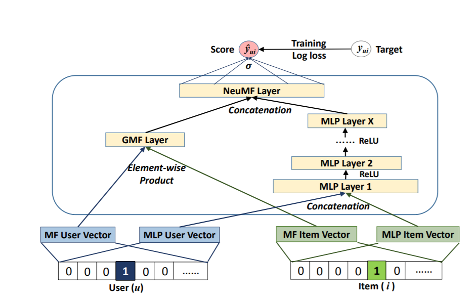
Why are neural recommender architectures (such as neural collaborative filtering) better than their traditional counterparts for handling sparsity?
- Neural recommender architectures, such as Neural Collaborative Filtering (NCF), often perform better than traditional recommendation methods, especially in handling sparsity. Here are some reasons why neural recommenders can be more effective:
Learning Complex Patterns
Neural networks are capable of learning complex, non-linear relationships between users and items. This ability to capture intricate patterns in the data helps in making more accurate recommendations, even when the data is sparse.
Better Generalization
Neural networks can generalize better from limited data. They can learn from the interactions present and infer preferences more effectively than traditional models like matrix factorization, which may struggle with high sparsity.
Flexible Representations
Neural recommenders can learn continuous, dense representations (embeddings) of users and items that encapsulate more information than the explicit interaction data. These embeddings capture latent factors that are not immediately obvious in the original sparse interaction matrix.
Handling Diverse Input Features
Neural architectures can easily incorporate a variety of input features, such as user demographics, item attributes, and contextual information (e.g., time, location). This flexibility allows them to leverage additional information to make better recommendations even when interaction data is sparse.
Deep Representation Learning
Deep learning models, including NCF, can stack multiple layers to learn hierarchical representations of data. This deep representation learning helps in capturing higher-order interactions between users and items, which is particularly useful in sparse datasets.
Comparison: Neural Collaborative Filtering vs. Matrix Factorization
Neural Collaborative Filtering (NCF)
- Architecture: Combines embeddings of users and items with neural network layers to model their interactions.
- Strengths:
- Can capture non-linear interactions.
- Incorporates multiple layers for deep feature learning.
- Easily integrates additional user and item features.
- Weaknesses:
- Requires more computational resources.
- Needs careful tuning of hyperparameters.
Traditional Matrix Factorization (MF)
- Architecture: Factorizes the user-item interaction matrix into latent factors for users and items.
- Strengths:
- Simple and interpretable.
- Efficient with dense data.
- Weaknesses:
- Assumes linear interactions.
- Struggles with high sparsity and cold-start problems.
- Limited in incorporating additional features.
Empirical Evidence
-
Several studies and practical implementations have shown that neural recommenders outperform traditional methods, especially in sparse datasets:
- He et al. (2017): The authors of the Neural Collaborative Filtering paper demonstrated that NCF outperformed matrix factorization on several benchmark datasets, particularly when the interaction data was sparse.
- He et al. (2018): The Neural Graph Collaborative Filtering (NGCF) paper showed that incorporating graph neural networks further improved performance, highlighting the advantage of using advanced neural architectures in recommendation systems.
Example: Implementing NCF in PyTorch
Here’s a simplified example of how you might implement a basic NCF model using PyTorch:
import torch
import torch.nn as nn

class NeuralCollaborativeFiltering(nn.Module):
    def __init__(self, num_users, num_items, embedding_dim, hidden_layers):
        super(NeuralCollaborativeFiltering, self).__init__()
        self.user_embedding = nn.Embedding(num_users, embedding_dim)
        self.item_embedding = nn.Embedding(num_items, embedding_dim)
        layers = []
        input_dim = 2 * embedding_dim
        for hidden_dim in hidden_layers:
            layers.append(nn.Linear(input_dim, hidden_dim))
            layers.append(nn.ReLU())
            input_dim = hidden_dim
        layers.append(nn.Linear(input_dim, 1))
        self.model = nn.Sequential(*layers)

    def forward(self, user_ids, item_ids):
        user_embeds = self.user_embedding(user_ids)
        item_embeds = self.item_embedding(item_ids)
        interaction = torch.cat([user_embeds, item_embeds], dim=-1)
        prediction = self.model(interaction)
        return prediction

# Example usage
num_users = 1000
num_items = 1000
embedding_dim = 64
hidden_layers = [128, 64]

model = NeuralCollaborativeFiltering(num_users, num_items, embedding_dim, hidden_layers)

user_ids = torch.LongTensor([1, 2, 3])
item_ids = torch.LongTensor([10, 20, 30])

# Forward pass
outputs = model(user_ids, item_ids)
print(outputs)
Conclusion
- Neural recommender systems, such as Neural Collaborative Filtering, are generally better at handling sparsity than traditional methods due to their ability to learn complex, non-linear interactions, generalize better from limited data, and incorporate a wide range of input features. They represent a powerful approach for building modern recommendation systems that need to operate effectively in sparse data environments.
How are Factorization Machines different from Deep Factorization Machines?
- Factorization Machines (FMs) and Deep Factorization Machines (DeepFM) are both powerful models used in recommendation systems, but they have distinct architectures and capabilities. Here’s a detailed comparison of the two:
Factorization Machines (FMs)
Architecture:
- Linear Terms: FMs include linear terms for the input features.
-
Pairwise Interactions: FMs model pairwise interactions between features using factorized parameters.
- Mathematical Representation:
- where:
- \(w_0\) is the global bias.
- \(w_i\) are the weights of the linear terms.
- \(\mathbf{v}_i\) and \(\mathbf{v}_j\) are the latent vectors for feature \(i\) and \(j\).
- \(\langle \mathbf{v}_i, \mathbf{v}_j \rangle\) represents the dot product of the latent vectors.
Strengths:
- Efficiency: FMs can model interactions between features efficiently even when the feature space is large.
- Interpretability: The interaction terms are interpretable as they explicitly model the pairwise interactions.
Limitations:
- Limited Complexity: FMs only capture pairwise interactions and may miss higher-order interactions present in the data.
Deep Factorization Machines (DeepFM)
- Architecture: DeepFM combines the strengths of Factorization Machines and deep neural networks to capture both low- and high-order feature interactions.
- FM Component:
- Similar to traditional FMs, this component models low-order (pairwise) feature interactions.
- Deep Component:
- A deep neural network (DNN) that captures high-order feature interactions.
- The input features are transformed into dense embeddings, which are then processed through multiple hidden layers.
-
Mathematical Representation: \(\hat{y}(\mathbf{x}) = \text{FM Component}(\mathbf{x}) + \text{Deep Component}(\mathbf{x})\)
- Components:
-
FM Component: \(\text{FM Component}(\mathbf{x}) = w_0 + \sum_{i=1}^{n} w_i x_i + \sum_{i=1}^{n} \sum_{j=i+1}^{n} \langle \mathbf{v}_i, \mathbf{v}_j \rangle x_i x_j\)
- Deep Component: \(\text{Deep Component}(\mathbf{x}) = \text{MLP}(\mathbf{e})\) where \(\mathbf{e}\) is the embedding of the input features and MLP (Multi-Layer Perceptron) is the neural network that captures high-order interactions.
Strengths:
- Captures High-Order Interactions: The deep component allows DeepFM to model complex interactions beyond pairwise.
- Combines Best of Both Worlds: Leverages the efficiency of FMs for low-order interactions and the power of DNNs for high-order interactions.
Limitations:
- Increased Complexity: More complex to train and tune compared to traditional FMs.
- Computational Cost: Higher computational cost due to the deep neural network component.
Example Comparison
Factorization Machine (FM) Example in PyTorch
import torch
import torch.nn as nn

class FactorizationMachine(nn.Module):
    def __init__(self, num_features, k):
        super(FactorizationMachine, self).__init__()
        self.num_features = num_features
        self.k = k
        self.linear = nn.Linear(num_features, 1)
        self.v = nn.Parameter(torch.randn(num_features, k))

    def forward(self, x):
        linear_part = self.linear(x)
        interaction_part = 0.5 * torch.sum(
            torch.pow(torch.mm(x, self.v), 2) - torch.mm(torch.pow(x, 2), torch.pow(self.v, 2)), dim=1, keepdim=True)
        output = linear_part + interaction_part
        return output

# Example usage
num_features = 10
k = 5
model = FactorizationMachine(num_features, k)
x = torch.randn(3, num_features)
output = model(x)
print(output)
DeepFM Example in PyTorch
import torch
import torch.nn as nn

class DeepFM(nn.Module):
    def __init__(self, num_features, embedding_dim, hidden_layers):
        super(DeepFM, self).__init__()
        self.num_features = num_features
        self.embedding_dim = embedding_dim

        # FM component
        self.linear = nn.Linear(num_features, 1)
        self.v = nn.Parameter(torch.randn(num_features, embedding_dim))

        # Deep component
        self.embeddings = nn.Embedding(num_features, embedding_dim)
        self.deep_network = nn.Sequential()
        input_dim = num_features * embedding_dim
        for hidden_dim in hidden_layers:
            self.deep_network.add_module('fc', nn.Linear(input_dim, hidden_dim))
            self.deep_network.add_module('relu', nn.ReLU())
            input_dim = hidden_dim
        self.deep_network.add_module('output', nn.Linear(input_dim, 1))

    def forward(self, x):
        # FM component
        linear_part = self.linear(x)
        interaction_part = 0.5 * torch.sum(
            torch.pow(torch.mm(x, self.v), 2) - torch.mm(torch.pow(x, 2), torch.pow(self.v, 2)), dim=1, keepdim=True)

        # Deep component
        embeds = self.embeddings(torch.argmax(x, dim=1))
        embeds = embeds.view(x.size(0), -1)
        deep_part = self.deep_network(embeds)

        output = linear_part + interaction_part + deep_part
        return output

# Example usage
num_features = 10
embedding_dim = 5
hidden_layers = [64, 32]

model = DeepFM(num_features, embedding_dim, hidden_layers)
x = torch.randn(3, num_features)
output = model(x)
print(output)
Summary
- Factorization Machines (FMs):
- Focus on modeling linear terms and pairwise feature interactions.
- Efficient and interpretable, but limited to pairwise interactions.
- DeepFM:
- Combines the strengths of FMs and deep neural networks.
- Models both low-order and high-order interactions.
- More complex but capable of capturing intricate patterns in the data.
- Neural recommender architectures like DeepFM provide a more comprehensive approach to modeling interactions in recommendation systems, particularly in handling sparsity and complex feature interactions.
In the context of recommender systems, are neural networks or traditional ML techniques better at handling sparsity?
- In the context of recommender systems, the ability to handle sparsity — a common issue where most users have only interacted with a small subset of items — varies between traditional machine learning (ML) techniques and neural networks. Here’s a comparative analysis:
Traditional ML Techniques
- Collaborative Filtering (CF) Algorithms:
- User-Based and Item-Based CF: These methods can struggle with sparsity because they rely on finding users or items with similar profiles. When data is sparse, finding these similarities becomes difficult.
- Matrix Factorization (e.g., SVD, ALS): These techniques decompose the user-item interaction matrix into lower-dimensional matrices, which can help alleviate sparsity issues by capturing latent factors. However, they still require a significant amount of data to accurately model interactions.
- Content-Based Filtering:
- This method leverages item attributes to recommend similar items. While it can mitigate sparsity issues to some extent, it requires rich metadata about the items, which might not always be available.
- Hybrid Methods:
- Combining CF and content-based filtering can improve performance in sparse environments by using content information to fill in gaps where collaborative data is lacking.
Neural Networks
- Neural Collaborative Filtering (NCF):
- NCF combines the strengths of neural networks with collaborative filtering. By learning nonlinear interactions between users and items, NCF can capture complex patterns that traditional methods might miss. It often handles sparsity better due to its ability to learn from the implicit feedback (e.g., clicks, views) rather than just explicit feedback (e.g., ratings).
- Autoencoders:
- These are used for collaborative filtering by reconstructing the user-item interaction matrix. Denoising autoencoders, in particular, can handle missing data effectively, making them well-suited for sparse environments.
- Recurrent Neural Networks (RNNs) and Convolutional Neural Networks (CNNs):
- RNNs can model sequential interactions and temporal patterns, while CNNs can capture local patterns in the user-item interaction matrix. Both can enhance recommendation quality in sparse settings by leveraging additional contextual or sequential data.
- Graph Neural Networks (GNNs):
- GNNs are effective for modeling relationships in user-item interaction graphs. They can propagate information across the graph, making them powerful for handling sparsity by considering indirect interactions.
Comparative Insights
- Traditional ML Techniques: Effective when the dataset is relatively dense or when there is rich metadata. Matrix factorization methods, while powerful, can struggle with extreme sparsity unless supplemented with additional information.
- Neural Networks: Generally better at handling sparsity due to their ability to learn complex patterns and leverage implicit feedback. Techniques like NCF, autoencoders, and GNNs are particularly effective in sparse environments.
Conclusion
- Neural networks tend to be more adept at handling sparsity in recommender systems compared to traditional ML techniques. Their ability to model complex interactions, leverage implicit feedback, and use auxiliary data (like temporal or contextual information) makes them a robust choice for sparse datasets. However, the choice of technique should be guided by the specific characteristics of the dataset and the computational resources available.
Can traditional ML algorithms (such as logistic regression) take as input both sparse and dense features?
- Yes, traditional machine learning (ML) algorithms, including logistic regression, can take as input both sparse and dense features. Here’s how this can be achieved and what to consider:
Input Handling
- Sparse Features:
- These features are often represented using sparse matrices (e.g., CSR, CSC formats in Python’s SciPy library), which are memory-efficient representations for data where most of the values are zero.
- Sparse features typically arise in contexts like text data (e.g., bag-of-words, TF-IDF representations), user-item interaction matrices, or categorical variables with many categories (one-hot encoding).
- Dense Features:
- These are regular numerical or categorical features that are often represented as dense matrices or arrays.
- Examples include continuous numerical variables (e.g., age, salary) or dense embeddings obtained from deep learning models.
Logistic Regression with Mixed Feature Types
- Feature Representation: Combine sparse and dense features into a single feature matrix before training the model.
- Libraries like SciPy and NumPy can handle the concatenation of sparse and dense matrices.
- In Python, you can use
scipy.sparse.hstackto horizontally stack sparse matrices and dense matrices.
- Preprocessing: Ensure that both types of features are appropriately scaled or normalized if necessary.
- Sparse features from text data can be preprocessed using methods like TF-IDF.
- Dense features might require normalization (e.g., standard scaling).
Example Workflow in Python
Here’s a basic example using Python with scikit-learn:
import numpy as np
from scipy.sparse import csr_matrix, hstack
from sklearn.linear_model import LogisticRegression
from sklearn.preprocessing import StandardScaler
from sklearn.pipeline import Pipeline
from sklearn.compose import ColumnTransformer

# Sample dense features (e.g., numerical data)
dense_features = np.array([[1.0, 2.0], [3.0, 4.0], [5.0, 6.0]])

# Sample sparse features (e.g., one-hot encoded categories or text data)
sparse_features = csr_matrix([[0, 1, 0], [1, 0, 0], [0, 0, 1]])

# Combine sparse and dense features
combined_features = hstack([sparse_features, dense_features])

# Define a logistic regression model
model = LogisticRegression()

# Fit the model
model.fit(combined_features, [0, 1, 0])

# Make predictions
predictions = model.predict(combined_features)
print(predictions)
Considerations
- Memory Efficiency: When dealing with very large sparse datasets, ensure that operations on the combined feature matrix are memory-efficient.
- Feature Scaling: Dense features often require scaling (e.g., StandardScaler) to ensure that they have similar ranges. This is less of an issue with sparse features where most values are zero.
- Pipeline Integration: Use pipelines to streamline preprocessing and model training.
ColumnTransformercan be useful for applying different preprocessing steps to sparse and dense features separately.
Conclusion
- Traditional ML algorithms like logistic regression can indeed handle both sparse and dense features effectively. By appropriately representing and preprocessing these features, you can leverage the strengths of both types of data in your models.