Primers • World Models: Rendering, Simulation, Planning, and JEPA
- Background: World Modeling
- Overview
- Vision-Language-Action Models (VLAs), World Action Models (WAMs), and World Models (WMs)
- WAMs as Predictive Policies
- Desiderata
- FLUX 3 Action: Video-Pretrained World-Action Control
- Overview
- Joint Prediction of Futures and Actions
- Flow Matching Across Video and Action Modalities
- Video-Heavy Pretraining and Action Midtraining
- Action Representations Across Embodiments
- Robot-Specific Fine-Tuning
- Receding-Horizon World-Action Control
- Distillation and the WAM Efficiency Problem
- Simulation Evaluation with RoboLab
- Simulation Versus Real-Robot Evidence
- Embodiment Adaptation and Data Efficiency
- Beyond Manipulation
- Significance
- Isaac 0.5: Semantic Percepts as a Predictive Control Representation
- Overview
- Future-Percept Prediction
- Shared Backbone for Perception, Reasoning, and Control
- Discrete and Continuous Action Interfaces
- Joint Training Objective
- Typed Multimodal Training Across Embodiments
- Cross-Embodiment Control
- Scaling Action-Free Video Against Teleoperation
- Implications for World-Model Scaling
- Significance
- Representation Carriers in WAMs
- Temporal Horizons
- Uncertainty, Belief States, and Risk
- Data and Evaluation
- Open Challenges for Prediction-Grounded Embodied Models
- Synthesis: From Reactive Policies to Predictive Embodied Models
- From Actions to Predicted Consequences
- FLUX 3 Action as a Generative WAM
- A Semantic Predictive Route
- Scaling Foresight into Control
- Scaling with Video, Interaction, and Robot Data
- Latent-Predictive and Generative Routes
- Amortized Prediction Versus Explicit Planning
- Toward Prediction-Grounded Control
- Foundations of World Modeling
- The Agent-World Loop
- Formal Definition of a World Model
- Renderer Paradigm
- Simulator Paradigm
- Planner Paradigm
- Desiderata for Effective World Models
- Representation Learning in World Models
- Temporal Abstraction and Dynamics
- Uncertainty and Partial Observability
- Object-Centric and Relational Structure
- Learning Paradigms for World Models
- Limitations of Existing Approaches
- Transition to the Main World-Model Paradigms
- Renderer World Models
- Renderer World Models as Generative Observation Models
- Interactive Renderer World Models
- Multimodal Driving Renderers
- Learned Latent Actions and Playable Worlds
- Diffusion Renderers as Game Engines
- Diffusion World Models for Agent Training
- Real-Time Open-World Rendering
- Commercial Text-to-Video Renderers
- Implementation Pattern for Interactive Renderers
- Failure Modes and Evaluation
- Relationship to JEPA
- Design Trade-offs and Evaluation
- Simulator World Models
- Neural Scene and Spatial State Representations
- Learned Physical Dynamics and Relational Simulation
- From Static Scene State to Dynamic State Transition
- Interaction Networks and Object-Relation Simulation
- Visual Interaction Networks and Simulation from Video
- Graph Network-Based Simulators
- MeshGraphNets and Scientific Simulation
- Implementation Pattern for Learned Physical Simulators
- Error Accumulation and Stabilization
- Relationship to Renderer Models and JEPA
- Simulator World Models: Evaluation, Interfaces, and Integration
- Planner World Models
- Latent Imagination and Model-Based Control
- Search, Task-Oriented Latent Models, and Scalable Control
- Planning-Relevant Models Rather than Complete Simulators
- MuZero and Search over Learned Latent States
- Model Predictive Control with Task-Oriented Latent Dynamics
- Sampling-Based Trajectory Optimization
- Scaling Task-Oriented Planning with TD-MPC2
- Discrete Latent Planning and DreamerV2
- Planning Architecture Trade-offs
- Evaluation and Failure Modes
- Planning Evaluation Should Match the Decision Loop
- Model Exploitation and Reward Misgeneralization
- Planning Horizon and Compounding Error
- Online Search versus Amortized Planning
- Data Efficiency and Imagination Efficiency
- Evaluation Criteria for Planner World Models
- Integration with Renderer and Simulator World Models
- Relationship to JEPA
- Joint-Embedding Predictive Architectures
- Overview
- Core Principle: Prediction in Representation Space
- Architectural Components
- Masking and Target Selection
- Comparison with Other Self-Supervised Objectives
- JEPA, Renderers, Simulators, and Planners
- Avoiding Representation Collapse
- Temporal and Sequential Extensions
- Multimodal and Cross-Domain Extensions
- From Representation Learning to World Modeling
- Image-Based Joint-Embedding Predictive Architecture (I-JEPA)
- Video JEPA and Scalable World Modeling
- From Spatial to Spatiotemporal Prediction
- Video Renderers versus Video Latent Simulators
- V-JEPA: Learning Dynamics from Video
- V-JEPA 2: Scaling to Internet Video
- Representation Learning at Scale
- Action-Free Pretraining
- Action-Conditioned Post-Training
- Planning in Latent Space
- Relation to 3D and Spatial World Generation
- Advantages over Generative Video Models
- Limitations and Challenges
- Transition to Advanced JEPA World Models
- Advanced JEPA World Models
- Implementation Details for JEPA-Based World Models
- Probabilistic and Energy-Based Interpretations of JEPA
- Energy-Based View of JEPA
- Predictive Information Perspective
- Deterministic vs Probabilistic Prediction
- Variational JEPA
- Latent State as a Predictive Information State
- Bayesian JEPA and Belief Updates
- Planning with Energy-Based Objectives
- Renderer, Simulator, and Planner Under Uncertainty
- Collapse and Information Geometry
- Relation to Generative Models
- Unifying View
- Overview
- References
- World-model framing and taxonomy
- Renderer world models and video generation
- Interactive renderer world models
- Simulator world models and spatial representations
- Learned physical simulators
- Planner world models and latent control
- World Action Models, VLAs, and predictive robot control
- Isaac 0.5, semantic world modeling, and embodied scaling
- Robot-policy evaluation and embodied benchmarks
- Core JEPA papers
- Advanced JEPA and latent world models
- Collapse prevention and embedding geometry
- Representation learning foundations
- Energy-based and probabilistic foundations
- Social-media discussions and talks
- Citation
Background: World Modeling
Overview
-
World modeling is the study of learning internal predictive representations of an environment so an agent can infer what is true now, what is likely to happen next, and what would happen under possible actions. A minimal world model can be written as a transition model over latent states:
\[\hat{z}_{t+1}=f_\theta(z_t,a_t)\]- where \(z_t\) is a compact representation of the current observation, \(a_t\) is an action, and \(\hat{z}_{t+1}\) is the predicted next latent state. World Models by Ha and Schmidhuber (2018) established the modern neural framing of learning compressed spatial and temporal representations that can support policy learning inside a learned model.
-
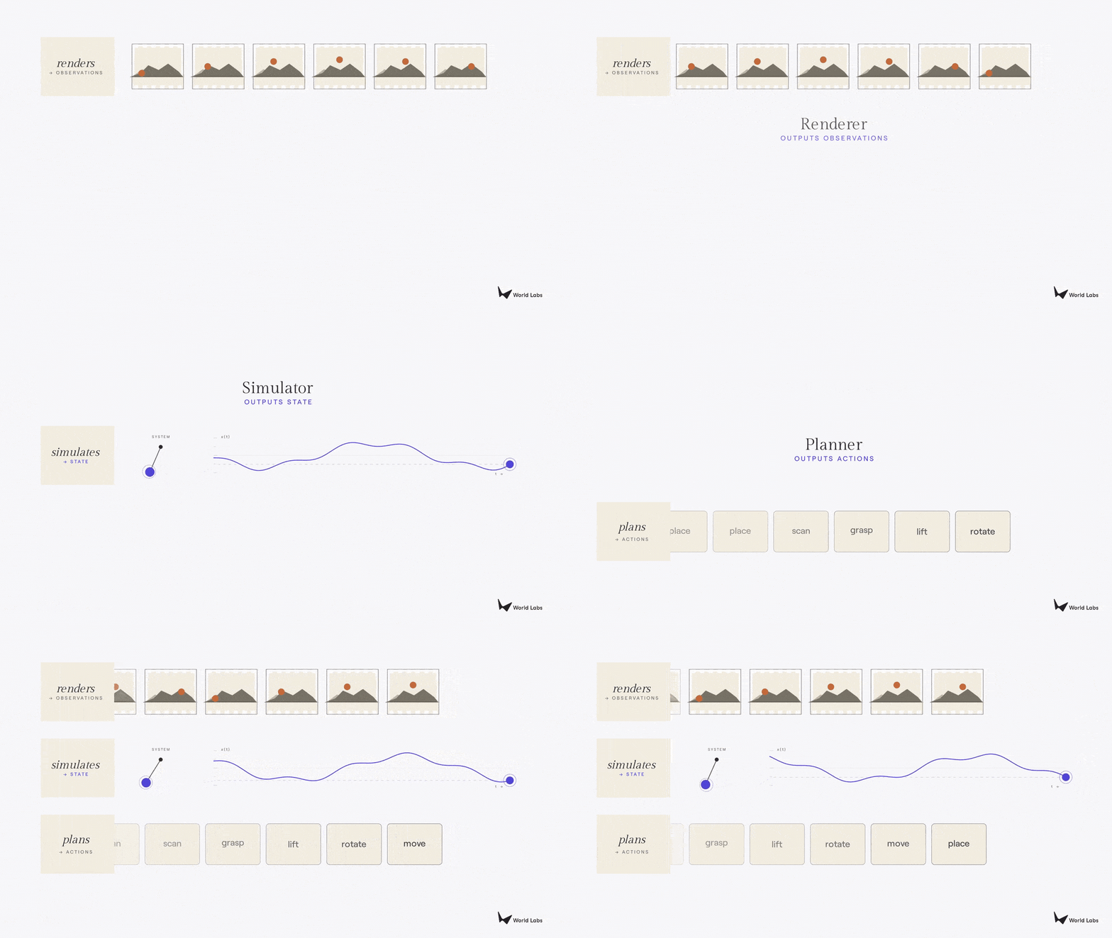
A more operational definition starts from the agent-environment loop: an agent selects actions, actions change the world state, observations expose only a partial view of that state, and new observations inform future actions. Reinforcement Learning: An Introduction by Sutton and Barto (2018) formalizes this loop through Markov decision processes and partially observable Markov decision processes, making it the control-theoretic substrate for most world-model definitions. A Functional Taxonomy of World Models distinguishes three outputs of this loop: renderers output observations, simulators output states, and planners output actions.
-
The following figure (source) shows a functional taxonomy in which renderers produce observations, simulators model state, and planners select actions.
Renderer World Models
-
Renderer-style world models generate observations, typically pixels, videos, or interactive views. Their primary contract is visual fidelity: given a prompt, state estimate, camera motion, or user input, they synthesize what an observer would see. This includes text-to-video and interactive generation systems, where the model may create plausible visual sequences without maintaining a fully explicit physical state. A Functional Taxonomy of World Models frames video models and interactive visual systems as renderers because their output is observation-level appearance rather than directly computable state.
-
Renderer models are valuable for imagination, visualization, and human-facing interaction, but visual plausibility is not the same as physical validity. A generated environment can look coherent while lacking metric geometry, stable object identity, or physically meaningful collision behavior.
Simulator World Models
-
Simulator-style world models output state: geometry, materials, object layouts, dynamics, or other representations that downstream programs can compute on. Their primary contract is structural fidelity rather than only visual fidelity. A simulator must support inspection, interaction, counterfactual evaluation, and repeated rollouts under intervention.
-
This paradigm includes classical physics engines, digital twins, robotics simulators, and newer generative 3D world models. Marble: A Multimodal World Model describes a multimodal system that creates editable 3D worlds from text, image, video, or coarse 3D layouts and exports worlds as Gaussian splats, meshes, or videos, illustrating the renderer-simulator boundary
-
Simulator world models are especially important for robotics, autonomous vehicles, engineering, game development, and scientific modeling because they provide a substrate for testing actions safely and cheaply before deployment.
Planner World Models
-
Planner-style world models output actions. Given an observation, a latent state, and a goal, a planner selects what should happen next:
\[a_t^*=\arg\min_{a_t} C(z_t,a_t,z_g)\]- where \(C\) is a goal-conditioned cost and \(z_g\) is a target state. Planners may use a learned dynamics model, a value function, search, model predictive control, or a policy network. Dream to Control: Learning Behaviors by Latent Imagination by Hafner et al. (2019) is a canonical example of learning compact latent dynamics and training behavior through imagined rollouts.
-
Planner world models close the perception-action loop. They are most directly connected to embodied AI because their output is not an image or a scene description, but an intervention in the world.
The Simulation Bottleneck
-
Among renderer, simulator, and planner paradigms, simulation is often the bottleneck because it links visual appearance to action consequences. A renderer can synthesize observations, and a planner can choose actions, but a simulator represents the structural substrate from which both visual observations and action-conditioned futures can be derived. A Functional Taxonomy of World Models argues that simulation is the bridge between rendering and planning because geometry, physics, and dynamics are the underlying structures needed by both.
-
This makes simulator-quality representations central to spatial intelligence. The challenge is that explicit 3D, material, physical, and robot-interaction data are far scarcer than internet-scale images and video, and generated 3D assets can look plausible while still containing scale errors, self-intersections, or physically invalid structure.
Toward Unified World Models
-
The strongest long-term direction is a unified model that can render observations, simulate state, and plan actions using shared latent knowledge. In such a system, a cup on a table would not merely be a texture pattern in pixels; it would have geometry, pose, material properties, affordances, and action-conditioned consequences.
-
The following figure (source) shows the convergence toward unified world models that combine rendering, simulation, and planning. Specifically, it shows a unified world-model architecture in which rendering produces interpretable observations, simulation maintains and evolves world state, and planning selects actions by evaluating predicted futures.

- This unified framing clarifies why world modeling is broader than video generation, robotics policy learning, or simulation alone. These are not isolated categories. They are projections of the same underlying problem: learning the structure of space, time, objects, dynamics, and agency.
JEPA as a Latent Predictive World Model
-
A central design question is whether the model should predict pixels, tokens, latent states, object slots, or task-relevant abstractions. Pixel-level generative models learn rich observation distributions, but they spend capacity on high-entropy details that may be irrelevant for planning, such as exact texture or background minutiae. JEPA-style models instead predict in representation space, biasing learning toward predictable semantic structure rather than full reconstruction. A Path Towards Autonomous Machine Intelligence by LeCun (2022) frames this as a path toward systems that learn predictive world models, reason, and plan through self-supervised learning rather than relying only on supervised labels or reinforcement rewards. (openreview.net)
-
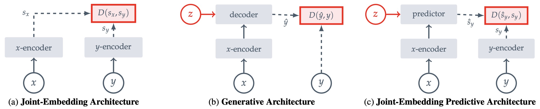
Joint-Embedding Predictive Architectures, or JEPAs, are a family of self-supervised models that learn by predicting the embedding of one signal from another compatible signal. Instead of reconstructing \(y\) directly, a JEPA learns encoders and a predictor such that:
\[s_x=f_\theta(x), \qquad s_y=f_{\bar{\theta}}(y), \qquad \hat{s}_y=g_\phi(s_x,z)\]-
and optimizes a latent prediction loss such as:
\[\mathcal{L}_{\text{JEPA}}=\left|\hat{s}_y-s_y\right|_2^2\]
-
-
The key shift is that compatibility is measured in embedding space rather than input space. Self-Supervised Learning from Images with a Joint-Embedding Predictive Architecture by Assran et al. (2023) introduced I-JEPA, where a Vision Transformer context encoder predicts representations of masked target blocks using an EMA target encoder and a predictor network.
-
The following figure (source) shows common architectures for self-supervised learning, in which the system learns to capture the relationships between its inputs. The objective is to assign a high energy (large scaler value) to incompatible inputs, and to assign a low energy (low scaler value) to compatible inputs. (a) Joint-Embedding Architectures learn to output similar embeddings for compatible inputs \(x, y\) and dissimilar embeddings for incompatible inputs. (b) Generative Architectures learn to directly reconstruct a signal \(y\) from a compatible signal \(x\), using a decoder network that is conditioned on additional (possibly latent) variables \(z\) to facilitate reconstruction. (c) Joint-Embedding Predictive Architectures learn to predict the embeddings of a signal \(y\) from a compatible signal \(x\), using a predictor network that is conditioned on additional (possibly latent) variables \(z\) to facilitate prediction.
-
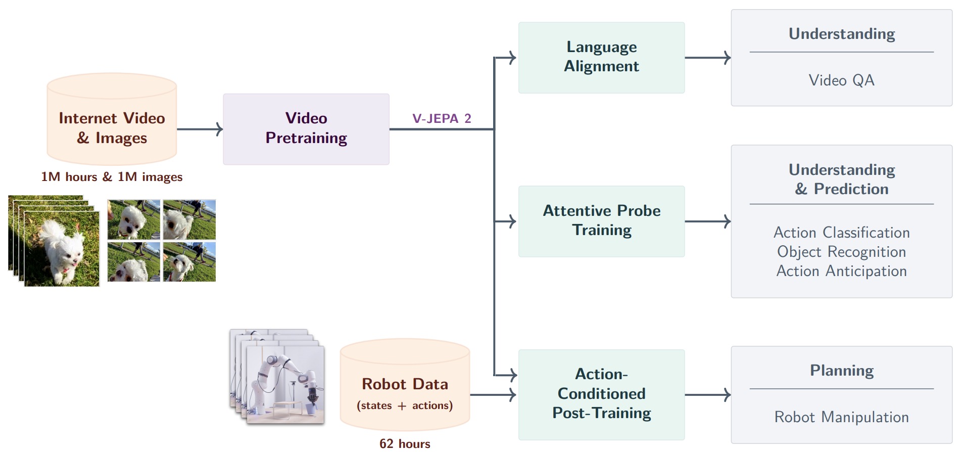
In world modeling, JEPA is best understood as a latent-space predictive model. Its appeal is that it can model the predictable consequences of perception and action without forcing the system to model every observation detail. In images, I-JEPA predicts masked spatial regions; in video, V-JEPA and V-JEPA 2 predict masked spatiotemporal regions; in robotics, action-conditioned variants predict future latent states conditioned on control inputs. V-JEPA 2: Self-Supervised Video Models Enable Understanding, Prediction and Planning by Assran et al. (2025) scales this recipe to internet-scale video and then post-trains an action-conditioned predictor with robot trajectories for planning.
-
The following figure (source shows the V-JEPA 2 training and deployment pipeline from large-scale video pretraining to downstream understanding and planning tasks. Specifically, large-scale video pretraining produces a video encoder for understanding and prediction, and action-conditioned post-training turns the frozen representation space into a planning-capable latent world model. Leveraging 1M hours of internet-scale video and 1M images, V-JEPA 2 is pretrained as a video model using a visual mask denoising objective, and this model is leveraged for downstream tasks such as action classification, object recognition, action anticipation, and Video Question Answering by aligning the model with an LLM backbone. After pretraining, we can also freeze the video encoder and train a new action-conditioned predictor with a small amount of robot interaction data on top of the learned representations, and leverage this action-conditioned model, V-JEPA 2-AC, for downstream robot manipulation tasks using planning within a model predictive control loop.
-
A practical JEPA implementation usually contains four components. First, an encoder maps observations into latent tokens. Second, a target encoder, often an exponential moving average of the context encoder, provides stable targets. Third, a predictor maps context representations, target-position tokens, temporal tokens, or action embeddings into predicted target representations. Fourth, an anti-collapse mechanism prevents the trivial solution where all inputs map to the same embedding. LeWorldModel: Stable End-to-End Joint-Embedding Predictive Architecture from Pixels by Maes et al. (2026) proposes an end-to-end JEPA from pixels with a next-embedding prediction loss plus a Gaussian latent regularizer.
-
The anti-collapse mechanism is not intrinsic to the JEPA architecture and can be implemented in different ways. EMA target encoders and stop-gradient create asymmetric learning dynamics that stabilize the prediction target, while explicit regularization constrains the geometry or distribution of the latent space itself. VICReg: Variance-Invariance-Covariance Regularization for Self-Supervised Learning by Bardes et al. (2022) prevents collapse by preserving per-coordinate variance and suppressing cross-coordinate covariance, whereas LeJEPA: Provable and Scalable Self-Supervised Learning Without the Heuristics by Balestriero and LeCun (2025) introduces SIGReg to match random projections of the embedding distribution to an isotropic Gaussian.
-
The core implementation distinction between generative world models and JEPA world models is therefore the training target:
- The second objective avoids an observation likelihood and directly trains the model to predict latent structure useful for perception, dynamics, and control. V-JEPA 2 by Assran et al. (2025) reports that this representation-space prediction supports motion understanding, action anticipation, video question answering after language alignment, and robot manipulation through latent model-predictive control.
Vision-Language-Action Models (VLAs), World Action Models (WAMs), and World Models (WMs)
-
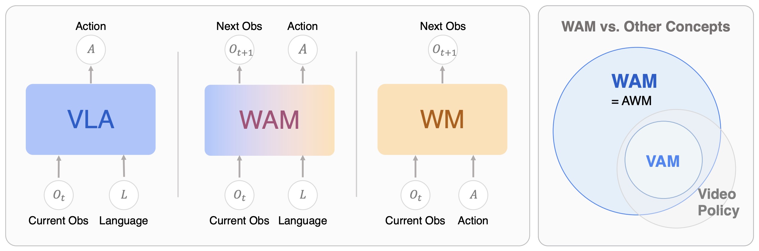
Vision-Language-Action models, World Action Models, and World Models are closely related, but they solve different parts of the embodied intelligence problem. A VLA is primarily a policy model: it maps perception and language to actions. A WM is primarily a predictive dynamics model: it maps a current state and a hypothetical action to a future state. A WAM combines these contracts: it predicts future world evolution and couples that prediction to action generation. RT-2: Vision-Language-Action Models Transfer Web Knowledge to Robotic Control by Brohan et al. (2023) introduced the VLA framing by representing robot actions as tokens in a vision-language model, while World Action Models: The Next Frontier in Embodied AI by Wang et al. (2026) formalizes WAMs as models that jointly predict future states and actions rather than actions alone.
-
A detailed discourse on Physical AI is available in our Physical AI primer.
-
The following figure (source) shows the conceptual definition and comparison of World Action Models, contrasting the input-output formulations of Vision-Language-Action models, World Action Models, and standard World Models, and showing that WAMs jointly predict actions and future observations.
-
A VLA models the conditional action distribution:
\[p_\theta(a_t \mid o_t, l)\]-
where \(o_t\) is the current observation, \(l\) is the language instruction, and \(a_t\) is the robot action. Its imitation-learning objective is typically:
\[\mathcal{L}_{\mathrm{VLA}} = \mathbb{E}_{(o_t,l,a_t)\sim \mathcal{D}} \left[ -\log p_\theta(a_t \mid o_t,l) \right]\]
-
-
This objective makes VLAs strong semantic policies because they inherit visual and linguistic abstractions from pretrained VLMs or LLMs, but it does not require the model to predict how the environment changes after an action. OpenVLA: An Open-Source Vision-Language-Action Model by Kim et al. (2024) trains an open 7B-parameter VLA on diverse robot demonstrations and emphasizes scalable fine-tuning for visuomotor control, while \(\pi_0\): A Vision-Language-Action Flow Model for General Robot Control by Black et al. (2024) attaches a flow-matching action model to a pretrained VLM for continuous robot control.
-
A WM models the conditional future-state distribution \(p_\phi(o_{t+1} \mid o_t,a_t)\) or, more commonly in latent-space systems \(p_\phi(z_{t+1} \mid z_t,a_t)\)
-
where \(z_t=f_\theta(o_{\leq t})\) is a compact latent state. Its objective can be written as:
\[\mathcal{L}_{\mathrm{WM}} = \mathbb{E}_{(o_t,a_t,o_{t+1})\sim \mathcal{D}} \left[ -\log p_\phi(o_{t+1}\mid o_t,a_t) \right]\]-
or as a latent transition loss:
\[\mathcal{L}_{\mathrm{latent}} = \mathbb{E} \left[ -\log p_\phi(z_{t+1}\mid z_t,a_t) \right]\]
-
-
-
World Models are therefore not necessarily policies. Their primary role is to support imagination, simulation, prediction, planning, or representation learning. World Models by Ha and Schmidhuber (2018) showed that compact spatial and temporal latent representations can support policy learning inside imagined rollouts, Learning Latent Dynamics for Planning from Pixels by Hafner et al. (2019) introduced PlaNet for online planning in learned latent dynamics, and Dream to Control: Learning Behaviors by Latent Imagination by Hafner et al. (2019) trained behaviors by propagating value gradients through imagined latent trajectories.
-
A WAM models the joint state-action distribution:
\[p_\psi(o_{t+1},a_t \mid o_t,l),\]-
with objective:
\[\mathcal{L}_{\mathrm{WAM}} = \mathbb{E}_{(o_t,l,o_{t+1},a_t)\sim \mathcal{D}} \left[ -\log p_\psi(o_{t+1},a_t\mid o_t,l) \right]\]
-
-
The defining property is not merely that a robot policy uses a video encoder or a dynamics representation. The defining property is that future-state prediction is part of the policy’s training or inference contract. In a WAM, action generation is constrained by anticipated world evolution, so the policy is no longer only reactive; it is predictive, counterfactual, and physically grounded. WorldVLA: Towards Autoregressive Action World Model by Cen et al. (2025) unifies future-image prediction and action generation in an autoregressive framework, while VLA-JEPA: Enhancing Vision-Language-Action Model with Latent World Model by Sun et al. (2026) uses latent future-state prediction to make VLA pretraining less dependent on pixel-level nuisance variation.
-
The WAM objective can be implemented in two broad ways. In a cascaded WAM, future-state prediction and action generation are factorized:
-
This design first imagines or retrieves a future state, then derives an action that moves the robot toward that state. Learning Universal Policies via Text-Guided Video Generation by Du et al. (2023) casts sequential decision-making as text-conditioned video generation and extracts control from generated video plans, while Video Language Planning by Du et al. (2023) uses text-to-video dynamics models and tree search to produce long-horizon video plans that can be translated into robot actions.
-
In a joint WAM, the future-state predictor and action generator are trained inside one shared model:
\[p_\psi(o_{t+1},a_t \mid o_t,l)\]-
or, in latent form:
\[p_\psi(z_{t+1},a_t \mid z_t,l)\]
-
-
This makes state prediction and action prediction mutually informative. The predicted future state improves action selection, while action prediction pressures the latent dynamics to preserve action-relevant physical structure. Video Prediction Policy: A Generalist Robot Policy with Predictive Visual Representations by Hu et al. (2024) conditions a robot policy on predictive visual representations learned by video diffusion models, and V-JEPA 2: Self-Supervised Video Models Enable Understanding, Prediction and Planning by Assran et al. (2025) shows how a video JEPA can be post-trained with a small amount of robot interaction data into an action-conditioned latent world model for planning.
-
The difference among the three model families can be summarized by their output contract:
- VLA: predicts \(a_t\) from \(o_t\) and \(l\). It is best understood as a language-conditioned robot policy.
- WM: predicts \(o_{t+1}\) or \(z_{t+1}\) from \(o_t\) or \(z_t\) and \(a_t\). It is best understood as a dynamics model that supports simulation or planning.
- WAM: predicts \(o_{t+1}\) or \(z_{t+1}\) together with \(a_t\) from \(o_t\) and \(l\). It is best understood as a predictive policy that couples world evolution with motor control.
-
This distinction matters because the models fail differently. A VLA may understand the instruction but choose an action that is physically brittle because it has not learned to forecast consequences. A WM may predict plausible futures but fail to produce executable actions because it is not trained as a policy. A WAM tries to reduce this gap by using future-state prediction as an intermediate or joint constraint on control. This makes WAMs especially relevant for long-horizon manipulation, deformable-object interaction, bimanual control, mobile manipulation, and tasks where the action must be chosen according to expected physical consequences rather than current appearance alone. Learning to Act from Actionless Videos through Dense Correspondences by Ko et al. (2023) illustrates the data advantage of this framing by extracting robot behavior from actionless video through synthesized execution and dense correspondences, showing why future-state prediction can make otherwise unlabeled video useful for control.
-
Within the broader taxonomy of world models, WAMs are closest to planner-style world models because their final purpose is action. However, they differ from classical planner world models because they are usually trained as embodied foundation models rather than task-specific model-based RL systems. They inherit the semantic grounding of VLAs, the dynamics prediction of WMs, and the action-generation objective of policies. Their long-term promise is therefore not merely better video prediction or better imitation learning, but a unified embodied model that can understand an instruction, imagine physically plausible futures, and select actions whose consequences are internally predicted before execution.
WAMs as Predictive Policies
-
A World Action Model can be understood as a planner-style world model whose predictive component is directly coupled to policy generation. Classical planner world models first learn or assume a dynamics model, then use search, model predictive control, value gradients, or policy optimization to choose actions. WAMs retain this predictive planning intuition, but they move it into an embodied foundation-model setting where language, perception, future-state prediction, and motor control are trained as parts of one policy-facing system. World Action Models: The Next Frontier in Embodied AI by Wang et al. (2026) formalizes this shift by defining WAMs as models of future states and actions rather than actions alone.
-
A reactive VLA policy can be written as:
\[a_{t:t+H} \sim p_\theta(a_{t:t+H} \mid o_{\leq t}, l)\]- where \(o_{\leq t}\) is the observation history, \(l\) is the language instruction, and \(a_{t:t+H}\) is an action chunk. This formulation is sufficient for imitation when the next action can be inferred from the current observation and instruction, but it does not require the model to represent what the world will look like after the action is executed. RT-2: Vision-Language-Action Models Transfer Web Knowledge to Robotic Control by Brohan et al. (2023) demonstrates the power of tokenized VLA policies by transferring web-scale vision-language knowledge into robot action generation, but its core policy contract remains observation-to-action prediction.
-
A classical planner world model instead separates dynamics prediction from action selection:
\[z_{t+1} \sim p_\phi(z_{t+1} \mid z_t, a_t)\] \[a_{t:t+H}^* = \arg\min_{a_{t:t+H}} \sum_{k=0}^{H} C(\hat{z}_{t+k}, a_{t+k}, z_g)\]- where \(z_t\) is the latent state, \(z_g\) is the goal representation, and \(C\) is a cost or energy function. Learning Latent Dynamics for Planning from Pixels by Hafner et al. (2019) introduced PlaNet as a model-based agent that learns latent dynamics from pixels and plans online in the learned latent space, while Dream to Control: Learning Behaviors by Latent Imagination by Hafner et al. (2019) trains behaviors by imagining trajectories in a compact latent world model.
-
A WAM collapses this separation by making future-state prediction part of the action model’s training or inference contract:
\[(\hat{z}_{t+1:t+H}, \hat{a}_{t:t+H}) \sim p_\psi(z_{t+1:t+H}, a_{t:t+H} \mid z_{\leq t}, l)\]-
or, in observation space:
\[(\hat{o}_{t+1:t+H}, \hat{a}_{t:t+H}) \sim p_\psi(o_{t+1:t+H}, a_{t:t+H} \mid o_{\leq t}, l)\]
-
-
This makes the action generator answer a stronger question than a VLA: not only “what action follows this instruction and observation?” but “what action follows this instruction and observation while producing a physically plausible future?” WorldVLA: Towards Autoregressive Action World Model by Cen et al. (2025) implements this idea autoregressively by unifying future-image prediction and action generation in one framework, showing that the world model and action model can mutually improve one another.
-
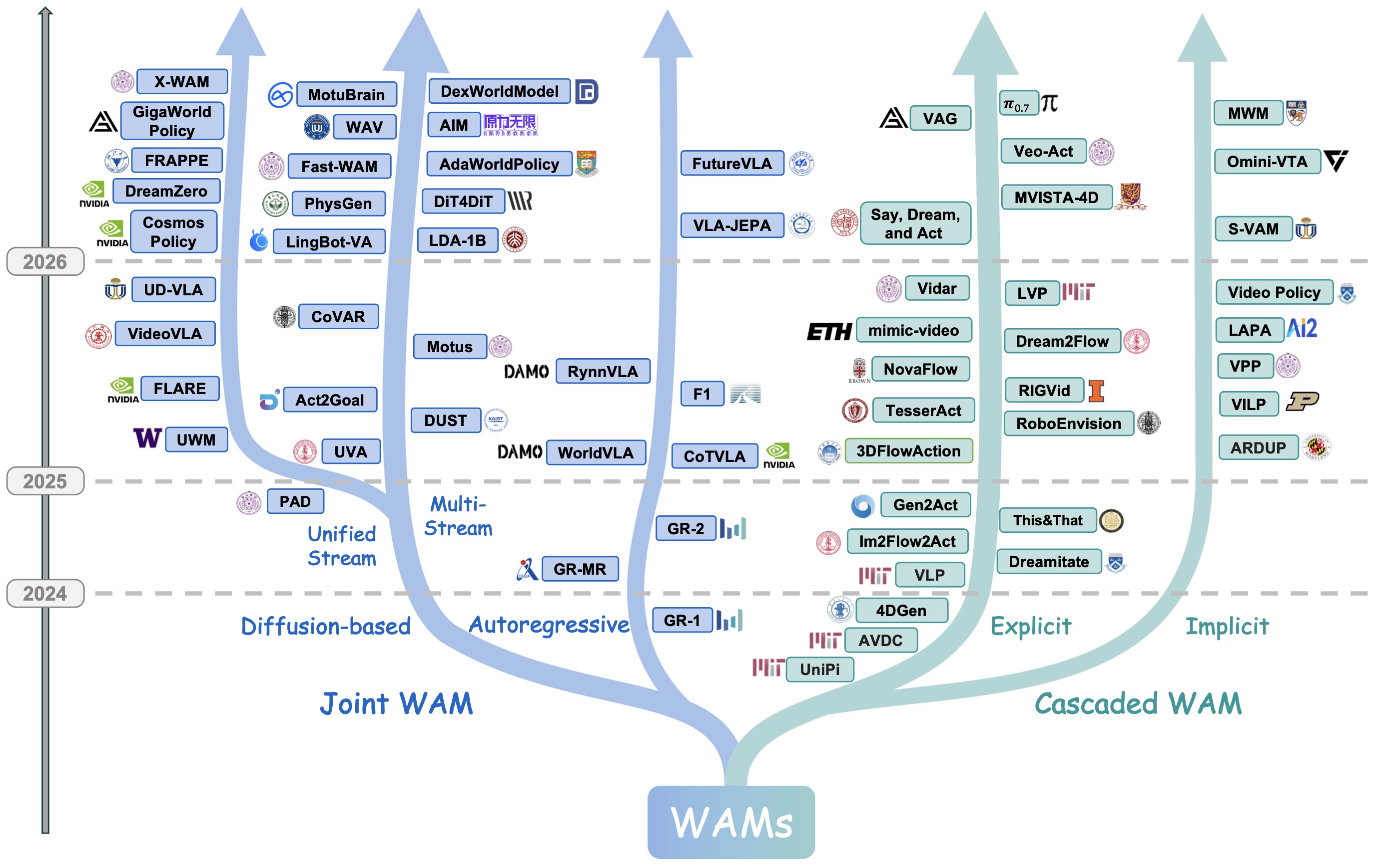
The following figure (source) shows the temporal evolution and taxonomy of representative World Action Models. The left branch illustrates Joint WAM architectures that tightly couple world prediction and action generation, while the right branch summarizes Cascaded WAM pipelines in which world modeling and action execution are more explicitly separated.
-
The most general WAM training objective can be decomposed into future prediction, action prediction, and consistency terms:
\[\mathcal{L}_{\mathrm{WAM}} = \mathcal{L}_{\mathrm{future}} + \lambda_a \mathcal{L}_{\mathrm{action}} + \lambda_c \mathcal{L}_{\mathrm{consistency}}\]-
where \(\lambda_a\) and \(\lambda_c\) control the relative weight of action supervision and prediction-action consistency. If the future is represented in pixel or video space, the future loss can be written as:
\[\mathcal{L}_{\mathrm{future\text{-}pixel}} = -\log p_\psi(o_{t+1:t+H} \mid o_{\leq t}, l)\]
-
-
If the future is represented in latent space, the future loss can instead be written as:
\[\mathcal{L}_{\mathrm{future\text{-}latent}} = \left\| \hat{z}_{t+1:t+H} - \bar{z}_{t+1:t+H} \right\|_2^2\]- where \(\bar{z}_{t+1:t+H}\) is a target representation produced by an encoder over future observations. VLA-JEPA: Enhancing Vision-Language-Action Model with Latent World Model by Sun et al. (2026) uses leakage-free latent future-state prediction to reduce sensitivity to appearance bias and nuisance motion in VLA pretraining.
-
The action loss depends on the action parameterization. For discrete action tokens, it is typically a negative log-likelihood:
- For continuous action chunks, it may be implemented through diffusion, flow matching, or regression over robot control trajectories. The consistency term encourages predicted actions and predicted futures to agree under a transition model:
-
This term is especially important when the future predictor can produce plausible-looking futures that are not actually reachable under the predicted robot actions. Video Prediction Policy: A Generalist Robot Policy with Predictive Visual Representations by Hu et al. (2024) conditions a robot policy on predictive visual representations from video diffusion models, illustrating how future-predictive representations can improve policy learning even when action execution remains policy-headed.
-
Cascaded WAMs make the planning structure explicit. They first synthesize or retrieve a future trajectory, then use that imagined trajectory as a goal or intermediate representation for control:
-
This is closest to classical visual planning because the generated future can be inspected, ranked, edited, or converted into subgoals before execution. Learning Universal Policies via Text-Guided Video Generation by Du et al. (2023) casts sequential decision-making as text-conditioned video generation and extracts control from generated video plans, while Video Language Planning by Du et al. (2023) uses text-to-video dynamics models with tree search to produce long-horizon video plans that can be translated into robot actions.
-
Joint WAMs instead train future prediction and action prediction in a shared representational space:
\[p_\psi(o_{t+1:t+H}, a_{t:t+H} \mid o_{\leq t}, l)\]-
or:
\[p_\psi(z_{t+1:t+H}, a_{t:t+H} \mid z_{\leq t}, l)\]
-
-
This design reduces the interface mismatch between a world model and a downstream policy, because the same backbone can learn which predicted future variables are action-relevant. The trade-off is that joint models may be harder to inspect than cascaded models, because their future predictions may appear as latent states, implicit visual features, or internal diffusion trajectories rather than directly viewable videos. WorldVLA: Towards Autoregressive Action World Model by Cen et al. (2025) is an autoregressive example of this joint direction, while VLA-JEPA: Enhancing Vision-Language-Action Model with Latent World Model by Sun et al. (2026) is a latent-predictive example that uses JEPA-style state prediction before action-head fine-tuning.
-
The conceptual boundary between WAMs and planner world models is therefore not whether both use prediction. Both do. The boundary is where action selection lives. In PlaNet, Dreamer, and TD-MPC-style systems, a learned world model supports a planner or policy optimizer that is usually trained for a control benchmark or task family. In WAMs, the predictive model is part of a broader embodied foundation model that is trained to connect language-conditioned intent, perceptual context, imagined future states, and action generation. TD-MPC2: Scalable, Robust World Models for Continuous Control by Hansen et al. (2024) scales model-predictive control in a learned latent world model across many continuous-control tasks, while WAMs extend the same prediction-for-control principle into multimodal robot foundation models.
-
This framing also clarifies the role of JEPA-style world models in robotics. A JEPA model predicts future representations rather than reconstructing pixels, so it can ignore visual details that are predictable but irrelevant to action. V-JEPA 2: Self-Supervised Video Models Enable Understanding, Prediction and Planning by Assran et al. (2025) pretrains a video JEPA on internet-scale video, then post-trains an action-conditioned predictor with robot trajectories to support planning in latent space. In a WAM context, this suggests a natural design: use JEPA-like latent prediction to learn physically meaningful future states, then condition action generation on those predicted states rather than on pixels alone.
-
The practical implication is that WAMs should be evaluated by the alignment between imagined futures and executed actions, not by future prediction or task success in isolation. A generated video that looks plausible is insufficient if the robot cannot execute the implied motion; a successful action is insufficient if it was selected by memorized dataset bias rather than grounded physical foresight. WAM evaluation therefore requires joint measurement of visual or latent future quality, physical plausibility, action feasibility, and causal agreement between predicted consequences and executed behavior. World Action Models: The Next Frontier in Embodied AI by Wang et al. (2026) explicitly organizes the WAM evaluation landscape around visual fidelity, physical commonsense, and action plausibility, which matches this joint prediction-control contract.
Desiderata
-
Effective embodied models should be evaluated according to the contract they claim to satisfy. A VLA should be judged primarily as a language-conditioned policy, a WM as a predictive dynamics model, and a WAM as a predictive policy that aligns future-state modeling with action generation. This distinction is important because the same architecture can appear strong under one contract and weak under another: a VLA may follow instructions without forecasting consequences, a WM may forecast plausible transitions without producing executable control, and a WAM may generate both actions and futures while still failing if the two are not physically consistent. RT-2: Vision-Language-Action Models Transfer Web Knowledge to Robotic Control by Brohan et al. (2023) frames robot actions as language-like tokens in a vision-language model, World Models by Ha and Schmidhuber (2018) frames control around compact predictive latent rollouts, and World Action Models: The Next Frontier in Embodied AI by Wang et al. (2026) defines WAMs as models that jointly characterize future states and actions rather than actions alone.
-
VLA desideratum: semantic grounding with reliable action execution. A VLA must ground language in visual observations and produce actions that are executable on a robot embodiment. Its key requirement is not only recognizing objects and instructions, but mapping them into temporally smooth control. A standard VLA training distribution can be written as:
\[\mathcal{D}_{\mathrm{VLA}} = \left\{(o_t,l,a_t)\right\}_{t=1}^{T}\]-
with an imitation-style objective:
\[\mathcal{L}_{\mathrm{VLA}} = \mathbb{E}_{(o_t,l,a_t)\sim\mathcal{D}_{\mathrm{VLA}}} \left[ -\log p_\theta(a_t\mid o_t,l) \right]\]
-
-
The desideratum is high conditional action accuracy under semantic variation:
-
This objective supports instruction following, object generalization, and embodiment transfer, but it does not by itself require the model to estimate whether the selected action will produce a physically valid future. OpenVLA: An Open-Source Vision-Language-Action Model by Kim et al. (2024) emphasizes scalable VLA training and fine-tuning across robot demonstrations, while \(\pi_0\): A Vision-Language-Action Flow Model for General Robot Control by Black et al. (2024) uses a flow-matching action expert on top of a pretrained VLM for continuous dexterous control.
-
WM desideratum: predictive sufficiency under intervention. A WM must preserve the variables needed to predict how the environment evolves when an action is applied. Its training distribution contains transitions:
\[\mathcal{D}_{\mathrm{WM}} =\left\{(o_t,a_t,o_{t+1})\right\}_{t=1}^{T}\]-
and the core objective is future-state prediction:
\[\mathcal{L}_{\mathrm{WM}} = \mathbb{E}_{(o_t,a_t,o_{t+1})\sim\mathcal{D}_{\mathrm{WM}}} \left[ -\log p_\phi(o_{t+1}\mid o_t,a_t) \right]\]
-
-
In latent-space systems, this becomes:
-
The desideratum is not raw reconstruction alone, but intervention fidelity: if the model is queried with counterfactual actions, the predicted future should change in the correct direction. This makes uncertainty, temporal consistency, object persistence, contact dynamics, and causal controllability more important than pixel-level sharpness in many robotics settings. Learning Latent Dynamics for Planning from Pixels by Hafner et al. (2019) learns latent dynamics for online planning, while V-JEPA 2: Self-Supervised Video Models Enable Understanding, Prediction and Planning by Assran et al. (2025) demonstrates that latent prediction over video can be post-trained with robot trajectories into an action-conditioned world model for planning.
-
WAM desideratum: consistency between imagined futures and executable actions. A WAM must satisfy both a predictive contract and a policy contract. Its training distribution contains language, observations, future states, and actions:
\[\mathcal{D}_{\mathrm{WAM}} = \left\{(o_t,l,o_{t+1:t+H},a_{t:t+H})\right\}_{t=1}^{T}\]-
and its objective can be written as:
\[\mathcal{L}_{\mathrm{WAM}} = \mathbb{E}_{\mathcal{D}_{\mathrm{WAM}}} \left[ -\log p_\psi(o_{t+1:t+H},a_{t:t+H}\mid o_{\leq t},l) \right]\]
-
-
Equivalently, a practical WAM objective can combine future prediction, action prediction, and action-future consistency:
- A useful consistency term checks whether predicted actions actually induce the predicted future under a learned or analytic transition model:
-
This term captures the key WAM desideratum: an imagined future should not merely be visually plausible, and an action should not merely imitate the dataset; the action and the imagined consequence should agree. WorldVLA: Towards Autoregressive Action World Model by Cen et al. (2025) trains future-image prediction and action generation in a shared autoregressive framework, while VLA-JEPA: Enhancing Vision-Language-Action Model with Latent World Model by Sun et al. (2026) uses leakage-free latent state prediction to learn action-relevant dynamics abstractions before action-head fine-tuning.
-
The data desiderata also differ across the three families. VLAs primarily need paired robot demonstrations with language or task labels, WMs need transition data with sufficient coverage of state changes, and WAMs need both action supervision and future-state supervision, or a training recipe that can combine actionless video with smaller amounts of robot interaction. This is why WAMs are attractive for scaling: they can inherit semantic priors from VLMs, learn temporal priors from internet-scale video, and use limited robot data to bind those priors to executable actions. Open X-Embodiment: Robotic Learning Datasets and RT-X Models by O’Neill et al. (2023) assembles cross-robot manipulation data for generalist policies, DROID: A Large-Scale In-The-Wild Robot Manipulation Dataset by Khazatsky et al. (2024) provides diverse real-world robot interaction trajectories, and V-JEPA 2 by Assran et al. (2025) shows how a large action-free video model can be adapted to robot planning with a comparatively small amount of robot trajectory data.
-
A concise way to state the difference is that VLAs optimize instruction-conditioned action likelihood, WMs optimize intervention-conditioned future likelihood, and WAMs optimize the compatibility of both:
- This comparison also clarifies evaluation. A VLA should be evaluated by task success, language grounding, embodiment transfer, action smoothness, and recovery from distribution shift. A WM should be evaluated by predictive accuracy, rollout stability, uncertainty calibration, causal validity, and usefulness for planning. A WAM should be evaluated by all of these, plus the alignment between predicted futures and executed actions. In practice, the hardest WAM failure mode is not poor video generation or poor action prediction in isolation, but a mismatch in which the model imagines a plausible future that its predicted action sequence cannot actually realize. World Action Models: The Next Frontier in Embodied AI by Wang et al. (2026) formalizes this issue by organizing WAMs around predictive state modeling coupled to action generation, and by separating evaluation into visual fidelity, physical commonsense, and action plausibility.
FLUX 3 Action: Video-Pretrained World-Action Control
Overview
-
FLUX 3 Action is a 7B-parameter World Action Model that maps visual observations, robot state, and a language instruction into both a future visual trajectory and a chunk of executable actions. Rather than treating video prediction and motor control as separate stages, the model denoises future video and action representations jointly, making it a direct realization of the joint-WAM formulation in which physical prediction and control share the same generative backbone.
-
The model is derived from the multimodal FLUX 3 foundation model, whose pretraining emphasizes video and treats images, video, audio, and actions as different observations of a common underlying physical process. Self-Supervised Flow Matching for Scalable Multi-Modal Synthesis by Chefer et al. (2026) introduces the Self-Flow training framework underlying this family, using heterogeneous corruption levels across modalities so that generative training simultaneously learns useful representations rather than only reconstructing corrupted inputs.
-
FLUX 3 Action therefore follows a different scaling hypothesis from conventional Vision-Language-Action models. Instead of requiring most physical knowledge to come from paired robot trajectories, it attempts to acquire dynamics priors from large-scale video and then bind those priors to control using a substantially smaller amount of action-labeled data. World Action Models Are Zero-Shot Policies by Ye et al. (2026) introduces DreamZero and similarly studies how pretrained video-diffusion models can transfer physical dynamics into robot policies through joint modeling of visual futures and actions.
Joint Prediction of Futures and Actions
- Let the current visual history be \(o_{\leq t}\), the robot state be \(s_t\), the language instruction be \(l\), the future visual trajectory be \(o_{t+1:t+H}\), and the action chunk be \(a_{t:t+K}\). FLUX 3 Action can be expressed at a high level as learning the joint conditional distribution:
- This differs from a conventional VLA, which need only estimate:
-
The explicit future-video term acts as an additional predictive constraint on the control policy. The model must not only infer what motion is associated with the instruction, but also learn an internal trajectory whose visual consequences are compatible with that motion. WorldVLA: Towards Autoregressive Action World Model by Cen et al. (2025) explores the same broader principle through autoregressive joint future-image and action prediction, whereas FLUX 3 Action implements joint prediction through a flow-matching generative process.
-
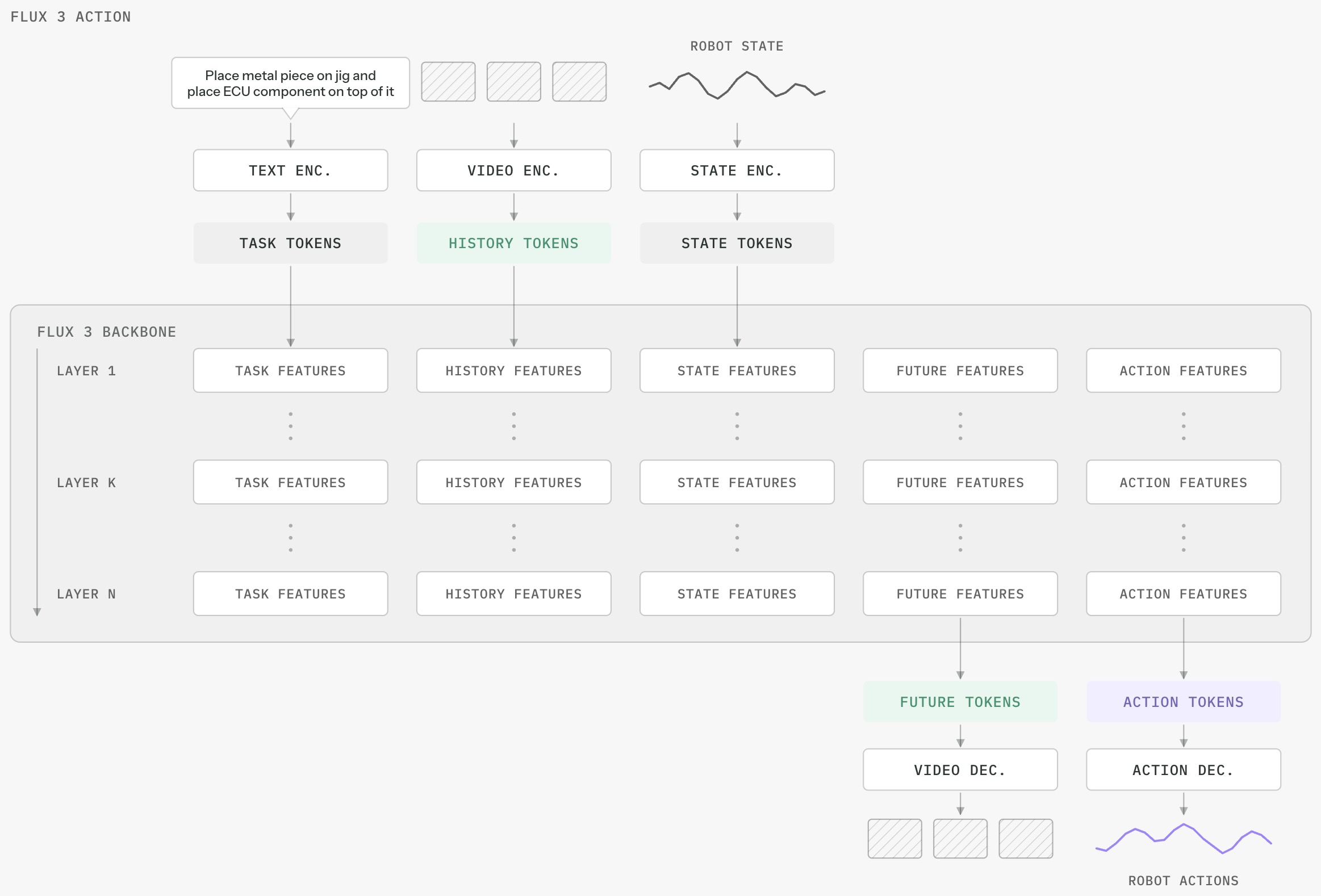
The following figure (source) shows the top-level architecture of FLUX 3 Action, which jointly predicts future video and robot actions, illustrating the defining WAM coupling between anticipated visual outcomes and executable control.
-
Architecturally, camera observations are encoded by a frozen video VAE, while language instructions are processed through a frozen Qwen3-VL-4B-Instruct-based text-conditioning pathway; robot-specific state and action representations are projected into the shared model through embodiment-specific interfaces. FLUX 3 Action describes the resulting system as a generative model in which video and actions remain jointly predicted instead of separating the world model from the action decoder.
-
The output interface is embodiment-specific rather than universal. A new robot may expose different joint coordinates, end-effector commands, gripper dimensions, or control rates, so the shared backbone can be retained while robot-specific conditioning projections and action heads translate between the embodiment and the common learned representation.
Flow Matching Across Video and Action Modalities
- FLUX 3 Action inherits a continuous generative formulation from the FLUX family. A simplified forward corruption process for a clean target \(x_0\) can be written as:
-
In the WAM setting, the clean target contains at least two jointly modeled modalities:
\[x_0 = \left[ v_0; a_0 \right]\]- where \(v_0\) denotes future video representations and \(a_0\) denotes future actions. The model therefore learns to reverse corruption over a state containing both what the world should look like and what the robot should do.
-
Joint denoising introduces an important optimization problem: video and actions have very different dimensionalities, statistics, and signal-to-noise transitions. FLUX 3 Action analyzes the reconstruction behavior of video and action modalities separately and finds that their useful denoising regions are not identical. FLUX 3 Action therefore evaluates multiple timestep distributions rather than assuming that a single uniform corruption schedule is equally appropriate for both modalities.
-
The model also scales the action representation before corruption. For an action scaling factor \(s\):
-
This changes where action information transitions between signal and noise relative to video. To avoid changing the effective optimization weighting merely because the representation has been rescaled, the action contribution can be reweighted proportionally to \(\frac{1}{s^2}\).
-
This provides a useful interpretation of modality coupling in generative WAMs. If action information becomes reliable earlier during generation than video information, visual prediction can increasingly condition on a relatively clean action trajectory. Conversely, shifting the relative signal-to-noise profiles in the other direction can make action generation depend more heavily on an emerging visual future.
-
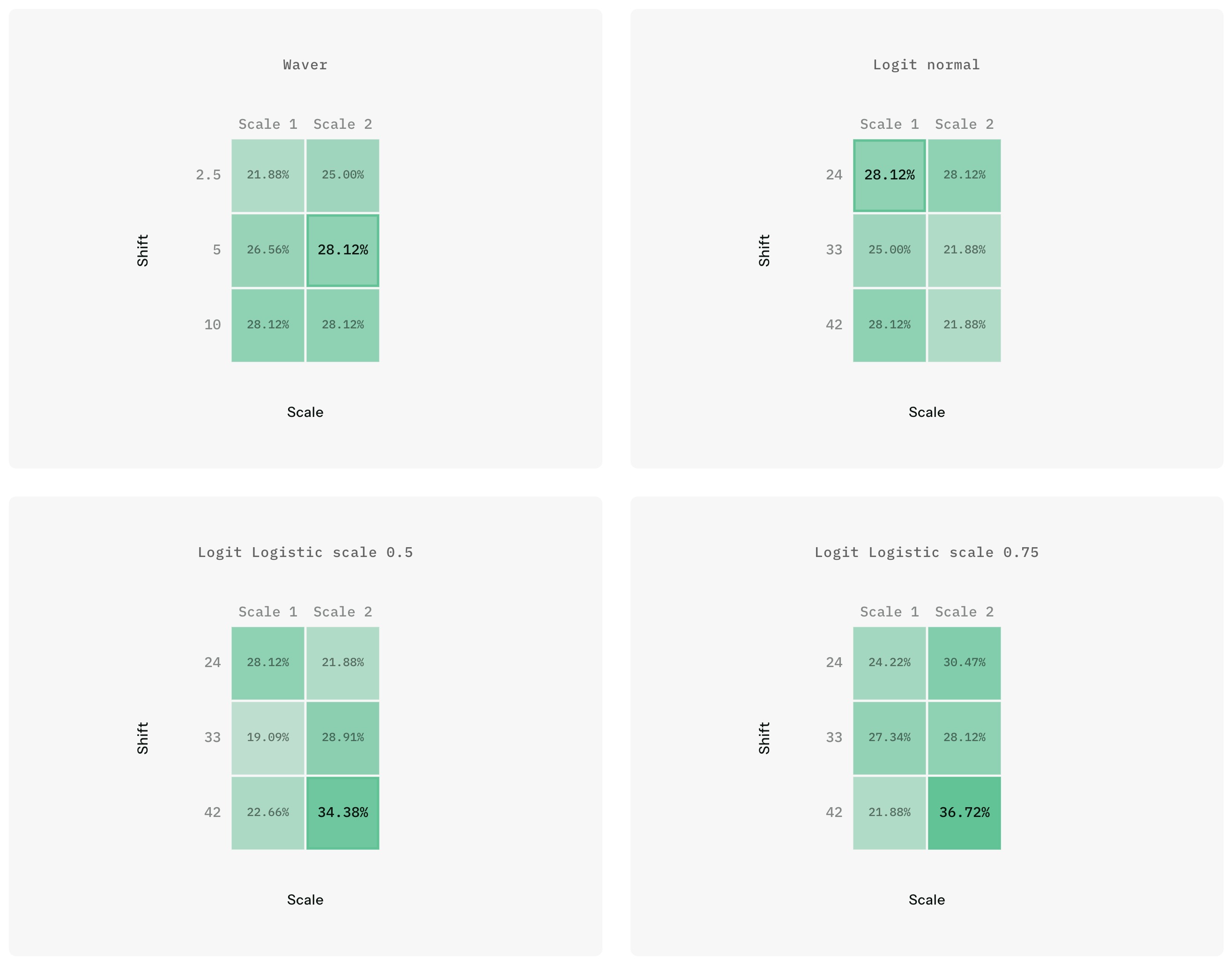
In the FLUX 3 Action experiments, logit-normal, logit-logistic, and Waver-style timestep distributions are evaluated together with different shifts and action scales. The strongest tested region consistently uses a logit-logistic distribution with action scaling \(s=2\) and a relatively high shift, motivating the configuration carried into later fine-tuning experiments.
-
The following figure (source) compares RoboLab success rates across timestep distributions, shifts, and action scales and illustrates how the joint video-action corruption schedule affects downstream robot-control quality.
Video-Heavy Pretraining and Action Midtraining
-
FLUX 3 Action makes the data-scaling argument for WAMs unusually explicit. Its initial FLUX 3 pretraining uses image, video, and audio data, with video accounting for more than 95% of the training tokens. The central premise is that temporal prediction forces the model to encode reusable information about motion, object persistence, causal relationships, interaction, and physical transformations before robot-specific supervision is introduced. FLUX 3 describes the broader FLUX 3 program as learning shared visual and multimodal representations across images, video, audio, and related modalities.
-
This pretraining is followed by action-oriented midtraining rather than immediately specializing on one robot. The reported training mixture assigns 36.95% of samples to video with audio and 63.05% to sources carrying aligned action information. Across the overall mixture, 19.55% of samples come from game recordings, 13.54% from egocentric videos with hand-pose annotations, 14.03% from handheld-gripper data, and 15.93% from teleoperation spanning 14 embodiments. FLUX 3 Action uses this mixture to broaden the definition of action supervision beyond conventional robot demonstrations.
-
The resulting hierarchy of supervision can be summarized as:
-
This hierarchy is important because robot demonstrations are expensive, while ordinary video, egocentric interaction footage, and game trajectories are comparatively abundant. The model attempts to learn generic temporal and action-conditioned structure from those broad sources before spending scarce robot data on embodiment calibration.
-
The pretraining ablations provide direct support for this strategy. When the robot action machinery is trained from random initialization using DROID fine-tuning, RoboLab performance remains below 1%; initializing from the video-heavy multimodal pretrained model produces a substantial increase, after which action midtraining continues to improve the initialization. DROID: A Large-Scale In-The-Wild Robot Manipulation Dataset by Khazatsky et al. (2024) supplies diverse real-world robot trajectories for the subsequent Franka-specific fine-tuning stage.
-
The following figure (source) shows RoboLab performance across random initialization, multimodal pretraining, and successive action-midtraining checkpoints, highlighting that video-heavy pretraining supplies much of the representation needed before robot-specific action learning.
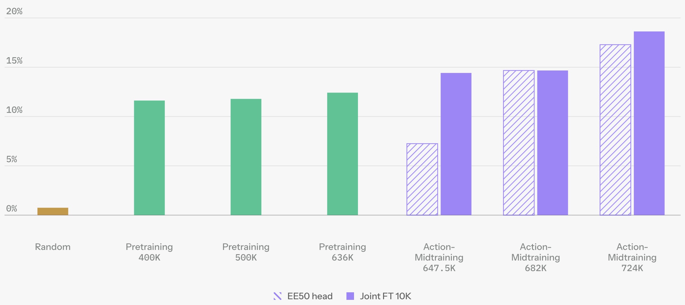
- In particular, the large gap between randomly initialized and pretrained models supports the broader WAM scaling hypothesis: action-labeled robot data does not need to carry the full burden of learning visual dynamics. A sufficiently strong video model can first learn regularities of temporal evolution, after which robot trajectories teach how those regularities relate to controllable intervention.
Action Representations Across Embodiments
-
Heterogeneous action datasets cannot be naively concatenated because robot embodiments expose incompatible control spaces. FLUX 3 Action addresses this during midtraining with standardized action parameterizations that can be selectively populated for each source.
-
One principal representation is an EE50 action space with 50 dimensions, divided into 25 dimensions for each of two possible end effectors. Each block contains translational coordinates, a continuous representation of orientation, and dimensions that can encode hand articulation or gripper state. Unused dimensions can be zero-padded, allowing single-arm, dual-arm, human-hand, and gripper-oriented examples to share a common intermediate interface.
-
The rotation representation follows the broader motivation of On the Continuity of Rotation Representations in Neural Networks by Zhou et al. (2019), which demonstrates that commonly used low-dimensional parameterizations of 3D rotation can introduce representational discontinuities and develops continuous alternatives that are better suited to neural prediction.
-
End-effector poses are expressed relative to an anchor state associated with the final conditioning frame rather than entirely in global coordinates. This turns the prediction target into a local motion trajectory and reduces sensitivity to embodiment-specific reference frames.
-
Gaming uses a distinct 102-dimensional representation containing discretized mouse displacement, mouse-button channels, and keyboard inputs. The inclusion of gaming is conceptually significant because it treats physical robotics and digital interaction as instances of the same visual-action prediction problem.
Robot-Specific Fine-Tuning
-
Robot adaptation occurs after multimodal pretraining and action midtraining. For the Franka embodiment used in DROID, FLUX 3 Action compares adaptation from its intermediate EE50 representation with fine-tuning in the robot’s joint-action space using newly initialized action heads.
-
A practical difficulty is that newly initialized embodiment-specific heads initially produce noisy gradients that can damage the pretrained world-action representation. The DROID recipe therefore freezes the pretrained weights for the first 1,000 steps, separately warms up the new action heads, and then gradually increases the learning rate applied to the pretrained trunk. FLUX 3 Action reports this staged adaptation as part of its fine-tuning recipe.
-
Larger-batch joint-space fine-tuning ultimately reaches higher RoboLab success than EE50 fine-tuning, while the pretrained EE50 interface remains attractive when adaptation data or training compute is highly constrained. This distinction suggests that a standardized action representation can improve fast embodiment transfer without necessarily being the optimal final action representation after sufficient target-robot optimization.
Receding-Horizon World-Action Control
-
At inference time, FLUX 3 Action uses closed-loop receding-horizon execution rather than committing to its full predicted trajectory. For the DROID configuration, one model invocation predicts 32 actions at 15 Hz, corresponding to approximately \(T_{\mathrm{chunk}} = \frac{32}{15} \approx 2.13\ \mathrm{s}\) of robot motion.
-
The model simultaneously maintains its video-prediction capability, although future video does not need to be decoded for every deployment. The robot executes only a configurable prefix of the action chunk, acquires fresh observations, and invokes the model again:
-
This design combines a relatively long internal prediction horizon with frequent external feedback. It therefore preserves some benefit from coherent world prediction without forcing the robot to trust the complete generated trajectory after the environment has changed.
-
Conceptually, this resembles model-predictive control, but the expensive optimization over candidate action sequences has been amortized into a learned world-action policy. Learning Latent Dynamics for Planning from Pixels by Hafner et al. (2019) uses explicit online planning over learned latent dynamics, whereas FLUX 3 Action directly generates a state-action trajectory and repeatedly refreshes that prediction from new observations.
Distillation and the WAM Efficiency Problem
-
Joint video-action prediction creates a computational disadvantage relative to action-only VLAs because a WAM must process the substantially longer token sequence associated with future visual states. Cosmos 3: Omnimodal World Models for Physical AI by NVIDIA et al. (2026) similarly combines multiple sensory and action modalities in an omnimodal physical-AI model, illustrating the expressive power as well as the computational cost of jointly modeling world evolution and action.
-
FLUX 3 Action addresses this cost without removing the interaction between video and action. Guidance distillation removes the need for a separate guidance evaluation, while subsequent step distillation compresses the sampling trajectory as far as a single generative step. The result exposes a central deployment trade-off:
\[\text{more denoising computation} \quad\Longleftrightarrow\quad \text{higher policy quality}\]- versus:
-
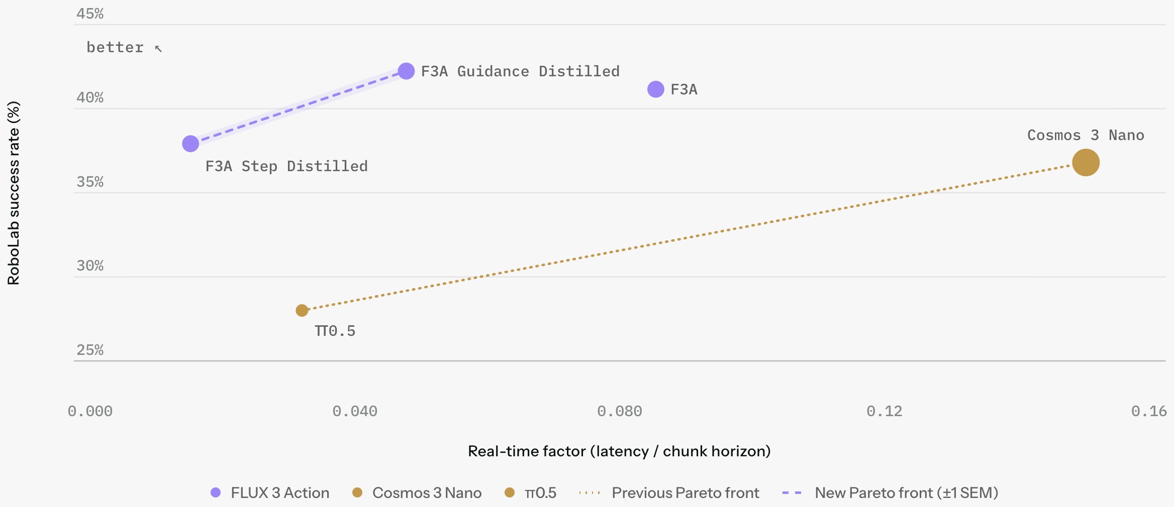
Importantly, the relevant efficiency measure for robotics is not merely model latency per invocation but processing time relative to the amount of physical motion produced. FLUX 3 Action predicts approximately \(2.13\) seconds of robot motion per call, whereas \(\pi_0.5\) predicts approximately \(1.0\) second under BFL’s comparison. \(\pi_0.5\): A Vision-Language-Action Model with Open-World Generalization by Physical Intelligence et al. (2025) provides the VLA baseline used in these comparisons.
-
On an NVIDIA B200, BFL reports 32.29 ms for the single-step FP8 FLUX 3 Action variant, compared with 31.99 ms for \(\pi_0.5\) in BF16 and 320.40 ms for the tested FP8 Cosmos 3 Nano configuration. FLUX 3 Action’s throughput advantage over \(\pi_0.5\) therefore does not come from substantially reducing per-call latency; it comes mainly from producing more robot-motion time per invocation.
-
The following figure (source) shows the RoboLab success-rate versus inference-speed trade-off across hardware and serving precisions. The plot highlights the Pareto trade-off between action-policy quality and processing cost and shows how guidance and step distillation move FLUX 3 Action toward the low-latency regime without removing joint video-action prediction.
Simulation Evaluation with RoboLab
-
FLUX 3 Action is evaluated extensively on RoboLab: A High-Fidelity Simulation Benchmark for Analysis of Task Generalist Policies by Yang et al. (2026), which evaluates generalist robot policies across 120 manipulation tasks designed to probe visual, relational, semantic, and procedural capabilities.
-
The principal FLUX 3 Action result reported by BFL is a 42.92% overall RoboLab-120 success rate. The corresponding release comparison reports 39.0% for OASIS WAM, 36.8% for Cosmos3-Nano-Policy, 28.0% for \(\pi_0.5\), 25.7% for DreamZero, and 7.2% for GR00T N1.6. FLUX 3 Action reports these figures together with policy type and parameter count.
-
The efficiency-optimized single-step checkpoint reaches approximately 38% RoboLab success while substantially reducing processing cost, whereas the guidance-distilled configuration reaches above 42%. This provides an unusually direct measurement of the accuracy-latency frontier within one WAM family rather than only between different model architectures.
-
Because RoboLab is a live benchmark, ordinal positions should be interpreted as snapshots rather than immutable properties of a model. Absolute success rate, model version, and evaluation conditions are more useful scientific descriptors than statements that a system is permanently “first” or “second.”
Simulation Versus Real-Robot Evidence
-
Simulation makes large-scale controlled evaluation practical, but it does not eliminate the sim-to-real gap. Small discrepancies in contact physics, camera calibration, friction, actuator behavior, deformable objects, and clutter can change policy behavior when transferred onto physical hardware.
-
RoboArena: Distributed Real-World Evaluation of Generalist Robot Policies by Atreya et al. (2025) addresses this broader evaluation problem by using distributed, blind real-robot comparisons rather than relying exclusively on simulated task completion.
-
FLUX 3 Action additionally reports an independent physical-robot evaluation conducted by Positronic Robotics using a Franka arm. Ten DROID-style single-object tasks were evaluated with three attempts per task under the same time limit and scoring procedure for each policy. FLUX 3 Action completed 28 of 30 attempts, compared with 27 of 30 for Cosmos 3 Nano, 20 of 30 for DreamZero, and 13 of 30 for \(\pi_0.5\). FLUX 3 Action reports that the operator was blinded to which policy controlled each attempt.
-
The following figure (source) shows a real-robot FLUX 3 Action rollout for the task “Put the cube in the bowl,” illustrating closed-loop execution of a manipulation behavior on a physical Franka robot.

- These results provide evidence that the simulation performance is not purely an artifact of RoboLab, but the physical evaluation remains much smaller than the space of conditions expected of a generalist embodied model. Thirty attempts across ten tasks cannot by themselves characterize robustness to clutter, lighting, novel geometry, contact-rich behavior, long-horizon composition, or hardware variation.
Embodiment Adaptation and Data Efficiency
-
The SO-101 experiments illustrate why the shared WAM backbone may be more consequential than any individual robot checkpoint. Once broad video-action structure has been learned, adaptation to a new embodiment becomes increasingly a problem of learning the correspondence between that embodiment’s observations, proprioceptive state, and control variables and the shared predictive representation.
-
This can be written as an embodiment-specific interface around a shared world-action model:
\[z_t = E_{\mathrm{obs}}^{(e)}(o_t,s_t)\] \[(\hat{z}_{t+1:t+H},\hat{u}_{t:t+K}) = F_\theta(z_t,l)\] \[\hat{a}_{t:t+K} = D_{\mathrm{act}}^{(e)}(\hat{u}_{t:t+K})\]- where \(e\) denotes the embodiment, \(F_\theta\) is the shared WAM backbone, and the observation and action adapters are embodiment-specific.
-
This decomposition is attractive because expensive world-model training can be amortized across embodiments. Robot-specific data then primarily needs to establish camera conventions, coordinates, kinematics, action semantics, control frequency, and actuator behavior rather than teaching generic temporal structure from scratch.
-
FLUX 3 Action applies the same general adaptation recipe to the low-cost SO-101 embodiment and evaluates not only in-distribution behaviors but also changes to objects, containers, and camera configuration. This is a more informative test of the shared representation than reproducing only the narrow conditions seen during teleoperation.
-
The following figure (source) presents SO-101 rollouts under out-of-distribution object changes and demonstrates how an embodiment-specific FLUX 3 Action policy behaves when manipulated objects differ from those represented in its fine-tuning distribution.

- Related WAM results provide complementary evidence for this scaling hypothesis. World Action Models Are Zero-Shot Policies by Ye et al. (2026) studies transfer from video-centric pretraining to robot policies and supports the broader idea that world-action representations can reduce the amount of embodiment-specific experience required for useful control.
Beyond Manipulation
-
FLUX 3 Action is not architecturally restricted to robot arms. The same action-prediction framework is tested on gaming data and explored for simulated navigation and control. FLUX 3 Action explicitly positions games as a useful testbed for action prediction and points toward computer-use and other latency-sensitive visually grounded agents.
-
This suggests a more general WAM formulation:
\[p_\theta \left( o_{t+1:t+H}, a_{t:t+K} \mid o_{\leq t}, s_t, l, e \right)\]- where \(e\) identifies the embodiment or action interface.
-
Under this interpretation, a robotic arm, drone, game controller, GUI agent, or autonomous vehicle differs substantially at the action boundary but shares a deeper computational problem: infer how a visually observed environment is likely to evolve under an intervention and choose an intervention that drives it toward a desired state.
Significance
-
FLUX 3 Action strengthens the case that generative video models can become control models without discarding their predictive visual objective. Instead of extracting static features from a pretrained video model and attaching a completely independent policy, the model retains world prediction and generates actions alongside the predicted future.
-
Its broader contribution is a practical WAM recipe in which:
- large-scale video-heavy multimodal pretraining learns transferable temporal and physical structure;
- heterogeneous action midtraining connects this representation to interaction across robots, human hands, handheld devices, and games;
- embodiment-specific fine-tuning specializes the shared representation to executable control;
- joint video-action prediction keeps future-state modeling inside the policy rather than relegating it to an external auxiliary model;
- receding-horizon execution converts multi-second action predictions into closed-loop behavior; and
- guidance and step distillation reduce the computational penalty associated with generating world evolution and actions jointly.
-
The remaining limitation is reliability. A RoboLab success rate of roughly 43% still leaves a large fraction of episodes unsuccessful, and simulated manipulation cannot fully reproduce the uncertainty, contact dynamics, clutter, hardware variation, and hidden state encountered by physical robots.
-
The deeper research question is therefore not whether video-pretrained WAMs can control robots, but how far predictive visual knowledge can substitute for expensive embodied interaction before failures in contact reasoning, partial observability, long-horizon decomposition, and uncertainty require richer state representations or explicit reasoning and planning.
-
In this sense, FLUX 3 Action occupies an important point between conventional VLAs and explicit world-model planners. It retains the amortized execution of a learned policy while requiring the policy to predict both action and anticipated world evolution. It therefore provides a concrete example of the central WAM thesis: scalable embodied intelligence may emerge more naturally when action is treated as another modality of world prediction rather than as an isolated output head.
Isaac 0.5: Semantic Percepts as a Predictive Control Representation
Overview
-
Isaac 0.5: Percepts Scale Control by Perceptron (2026) introduces a 36B-parameter open-weight embodied foundation model that trains video perception, embodied visual reasoning, semantic future prediction, and robot control through one shared sparse backbone. Rather than attaching a policy to a frozen visual encoder, Isaac 0.5 allows supervision from video, language, grounding, and actions to modify the same representation consumed by its control interfaces; Introducing Isaac 0.5 describes the system as spanning video understanding, embodied reasoning, and control across more than 35 robot systems.
-
Isaac 0.5 is especially relevant to world modeling because it introduces a third predictive target between two common extremes. Pixel-generative world models predict the future observation itself, while JEPA-style models predict a learned future embedding. Isaac 0.5 instead predicts a semantic future percept: a task-relevant visible state or change such as an object state, spatial relation, affordance, task phase, visible contact change, or likely near-future task state. Isaac 0.5: Percepts Scale Control by Perceptron (2026) uses this self-supervised future-percept objective to learn from action-free video without requiring human action labels or robot proprioception.
-
The model therefore occupies a useful position between a conventional VLA and a full generative WAM. It does not jointly render an explicit future video and action sequence as FLUX 3 Action does, but it also does not train control only from current observations. Instead, future-oriented semantic prediction shapes the shared state from which both autoregressive action tokens and continuous action chunks are produced. This makes Isaac 0.5 a prediction-grounded embodied model whose world-modeling target is task-relevant semantic change rather than complete observation reconstruction.
Future-Percept Prediction
- Let the observation history through time \(t\) be \(o_{\leq t}\) and let \(z_{t+\Delta}\) denote a semantic target derived automatically from a future observation at offset \(\Delta>0\). The disclosed future-percept objective is:
-
Here, \(g_\theta\) is the semantic predictor and \(\ell\) is the percept-prediction loss. Isaac 0.5: Percepts Scale Control by Perceptron (2026) explicitly leaves both the generator that constructs \(z_{t+\Delta}\) and the internal implementation of \(\ell\) proprietary, so the public objective specifies what is predicted but not the full target-construction pipeline.
-
The distinction between a percept and a conventional latent embedding is conceptual as well as operational. A generic latent predictor may optimize geometric closeness in an encoder-defined space:
whereas a semantic percept objective asks the model to predict task-relevant visible state change. V-JEPA 2: Self-Supervised Video Models Enable Understanding, Prediction and Planning by Assran et al. (2025) predicts future representations in learned embedding space and later adds action conditioning for planning; Isaac 0.5 instead makes semantic future prediction one cotraining objective of the same backbone that directly supports control.
- This yields a three-way spectrum of predictive targets:
- Pixel prediction preserves maximal observable detail but spends capacity on nuisance appearance; latent prediction compresses away observation detail but can be difficult to interpret; semantic percept prediction attempts to preserve explicitly task-relevant visible change without requiring the model to reconstruct the full visual future. Introducing Isaac 0.5 describes percepts as sitting between pixels and actions and emphasizes that their supervision is constructed automatically from future observations.
Shared Backbone for Perception, Reasoning, and Control
-
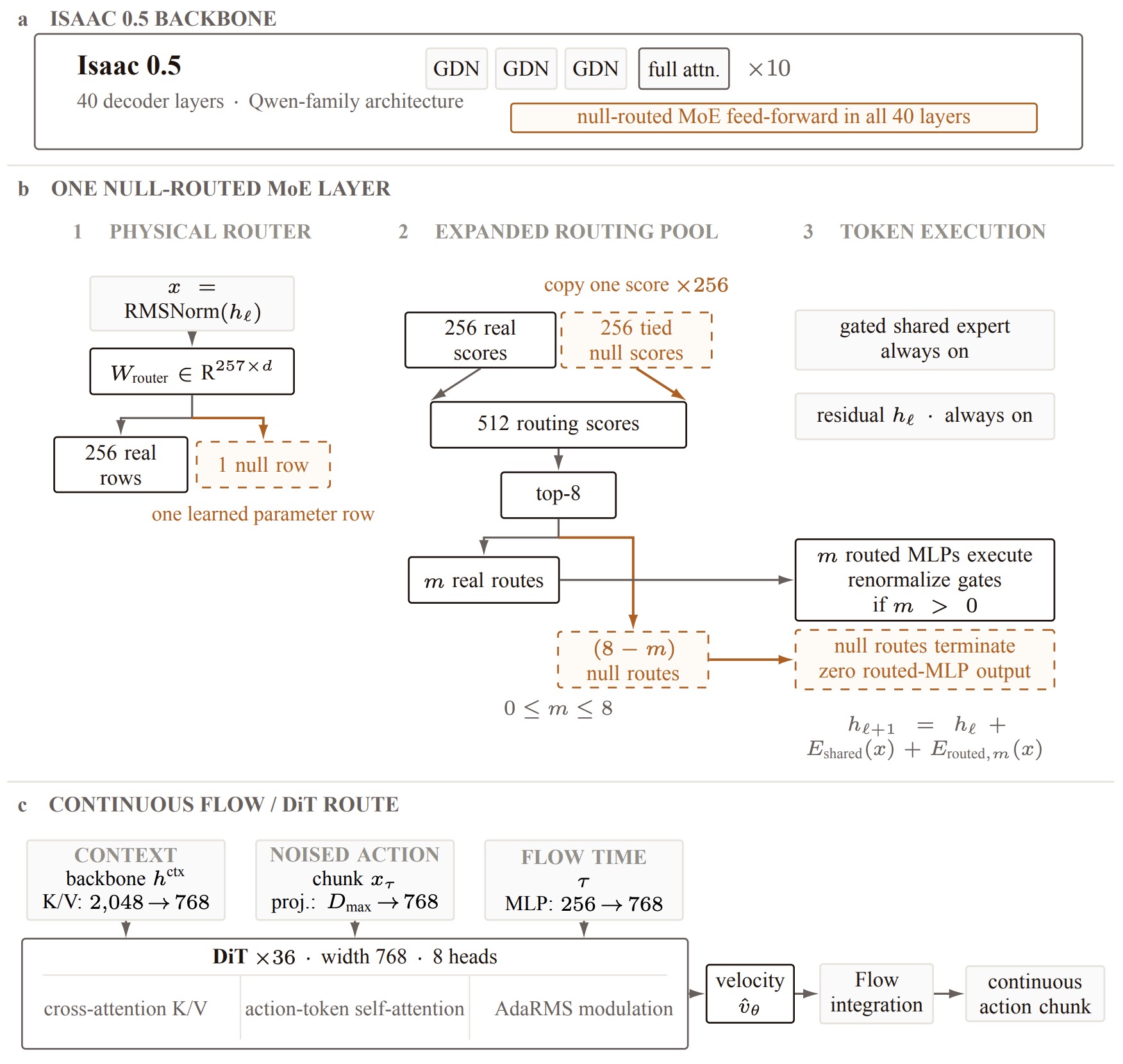
Isaac 0.5 uses a Qwen-family sparse vision-language backbone with 40 decoder blocks, comprising 30 GDN linear-attention blocks and 10 full-attention blocks. Every block contains 256 routed MLP experts, an always-on shared expert, and a learned null route that can occupy routing slots without executing a routed MLP. Isaac 0.5: Percepts Scale Control by Perceptron (2026) reports 36B total parameters and approximately 2.5B active parameters per token at its 50% null-routing reference point.
-
The routing mechanism lets each token execute between zero and eight real routed experts:
where \(m(x)\) is the number of real expert routes selected for token \(x\). Improving MoE Compute Efficiency by Composing Weight and Data Sparsity by Kilian et al. (2026) develops the zero-compute null-expert mechanism used to make token-choice MoE compute input-dependent while preserving causal autoregressive routing.
- This architecture is particularly well matched to embodied multimodality because a sequence may contain text, image patches, temporal markers, robot state, previous actions, and control targets with very different computational requirements. Null routing does not reduce the model’s stored weight memory, but it permits tokens to consume different amounts of routed feed-forward computation while retaining access to the full expert pool. Isaac 0.5: Percepts Scale Control by Perceptron (2026) reports that learned routing allocation varies substantially across task families and is concentrated most strongly during prompt processing.
The following figure (source) shows Figure 3, “Token-adaptive null routing and the continuous-control DiT.” The shared sparse block can skip routed MLPs through null routes, while the continuous-control DiT cross-attends to the backbone context and predicts a velocity field whose integration yields a continuous action chunk.
-
Null-expert routing also suggests a broader architectural principle for multimodal world models: representation capacity and inference compute need not be allocated uniformly across token types. If \(m(x)\) denotes the number of real routed experts selected for token \(x\), routed feed-forward computation can be viewed schematically as:
\[C_{\mathrm{routed}}(x) \propto m(x), \qquad 0 \leq m(x) \leq 8\]- so text, visual observations, robot state, action history, and predictive-control tokens can consume different amounts of expert computation inside the same sequence. Improving MoE Compute Efficiency by Composing Weight and Data Sparsity by Kilian et al. (2026) develops zero-compute null experts, while Isaac 0.5: Percepts Scale Control by Perceptron (2026) applies this mechanism throughout a shared embodied backbone containing language, vision, state, and action information.
-
This makes adaptive computation complementary to predictive-representation design. A world model may use pixels, semantic percepts, latent states, or joint state-action streams as its predictive carrier while independently learning how much routed computation each token requires. Null routing therefore changes active computation rather than model storage: the full expert pool remains available, but easy or redundant tokens can bypass routed MLP work while more demanding embodied context can activate additional experts.
Discrete and Continuous Action Interfaces
-
Isaac 0.5 exposes two complementary control paths from the same backbone state. Its autoregressive route uses a disjoint FAST action vocabulary alongside language, coordinates, and grounding outputs. FAST: Efficient Action Tokenization for Vision-Language-Action Models by Pertsch et al. (2025) compresses continuous action trajectories into frequency-space tokens so that high-frequency robot behavior can be learned by an autoregressive sequence model.
-
If \(a\) denotes a normalized action chunk and \(q=\operatorname{FAST}(a)\) its tokenized representation, the discrete control objective is:
where \(c\) is the shared-backbone context. Isaac 0.5: Percepts Scale Control by Perceptron (2026) includes FAST action positions inside the model’s broader next-token objective rather than optimizing them through a separate detached policy.
-
The continuous route uses a dedicated 36-block diffusion transformer conditioned on the same backbone representation. Scalable Diffusion Models with Transformers by Peebles and Xie (2022) introduced the DiT architecture, while Flow Matching for Generative Modeling by Lipman et al. (2023) formulates continuous generative modeling as vector-field regression along probability paths.
-
For action chunk \(a\), Isaac samples noise \(\epsilon_s\) and a noise level \(\tau_s\), constructs a noisy action \(x_s\), and trains the Flow expert to recover the constant straight-path velocity:
- The corresponding masked Flow objective is:
where \(S=4\) independent Flow-time samples are drawn per action chunk during training and \(M\) masks padded time steps and unused action dimensions. Isaac 0.5: Percepts Scale Control by Perceptron (2026) uses ten explicit Euler integration steps for this continuous route at inference.
- The architectural point is not merely that Isaac supports two action encodings. Both action routes read a context learned jointly from future-percept prediction, video understanding, grounding, and embodied reasoning. The control head therefore receives a representation that has already been pressured to encode what is likely to change in the world, rather than only what is visible in the present observation.
Joint Training Objective
- The shared representation is enforced through cotraining rather than through a frozen perception stack. At the disclosed level, the full training loss is:
-
Here, \(\mathcal{L}_{\mathrm{NTP}}\) covers eligible autoregressive language, grounding, reasoning, coordinate, control, and FAST positions; \(\mathcal{L}_{\mathrm{sem}}\) is future-percept prediction; \(\mathcal{L}_{\mathrm{Flow}}\) supervises continuous action chunks; and the remaining terms regularize language logits and sparse routing. Isaac 0.5: Percepts Scale Control by Perceptron (2026) emphasizes that these objectives update the shared backbone rather than insulating action generation from perception and semantic prediction.
-
This differs from a pipeline in which a pretrained visual representation is frozen and an action head is learned afterward:
- Isaac instead follows a cotrained pathway:
so the representation that supports action is directly altered by prediction and perception supervision.
Typed Multimodal Training Across Embodiments
-
Heterogeneous video and robot datasets do not expose the same fields. General video has visual time but no robot state; pointing data may contain coordinates but no actions; teleoperation trajectories contain camera observations, proprioception, and embodiment-specific controls; continuous action chunks cannot safely be treated as ordinary text tokens. Isaac 0.5: Percepts Scale Control by Perceptron (2026) addresses this through mHarmony, a typed compiler that validates source schemas, resolves embodiment-specific state and coordinate conventions, aligns clocks, and lowers heterogeneous examples into TensorStream events.
-
Each event retains modality, time, provenance, and embodiment information so that unrelated missing fields are not interpreted as negative supervision. Text, image and video blocks, temporal information, robot state, coordinates, and FAST actions can enter one packed sequence, while continuous Flow targets remain keyed outside the token stream but share observation identifiers with the sequence. This preserves a common representation without pretending that every data source provides the same supervision.
The following figure (source) shows Figure 5, “From heterogeneous experience to one model.” General video, egocentric and UMI data, teleoperation, and language/spatial examples are lowered through mHarmony into typed events before entering the shared Isaac 0.5 backbone and its perception, reasoning, FAST, and Flow interfaces.
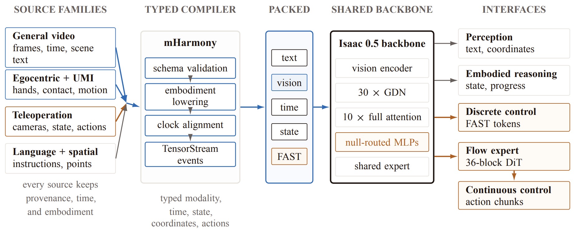
Cross-Embodiment Control
-
The released checkpoint covers more than 35 robot interface configurations, with robot-specific observation, action, normalization, timing, and safety configurations. Isaac 0.5: Percepts Scale Control by Perceptron (2026) demonstrates the same checkpoint executing the same cup-stacking request on YAM and SO-101 hardware by changing the embodiment identifier in the configuration prompt rather than swapping the core model.
-
This makes embodiment conditioning part of the model interface rather than requiring a separate foundation model for each robot. The shared backbone can be written schematically as:
where \(e\) identifies the embodiment and control configuration. The discrete or continuous action interface then maps the shared state into the embodiment-specific control representation:
\[\hat{a}_{t:t+K} = D^{(e)}(h_t)\]The following figure (source) shows Figure 4, “One checkpoint executes the same task on two physical embodiments by changing only the embodiment string in the configuration prompt,” with paired YAM and SO-101 rollouts at the initial reach, intermediate placement, and completed cup stack.
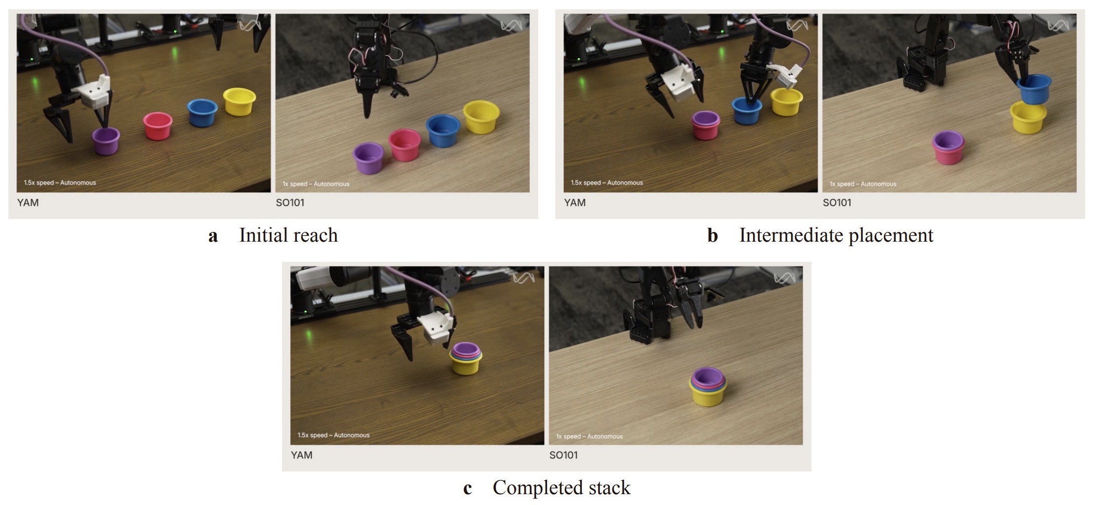
Scaling Action-Free Video Against Teleoperation
-
The central scaling experiment asks whether abundant action-free video can reduce the amount of expensive teleoperation required for control learning. Isaac 0.5 holds the general-video:egocentric:UMI source-hour ratio at \(80:30:30\) while varying the video scale against teleoperation and evaluating held-out action loss. Introducing Isaac 0.5 summarizes this as a scaling law for choosing the mix of video and robot demonstrations under a fixed budget and action-loss target.
-
For the primary offline action-loss threshold \(\tau=2.50\), increasing general video from \(1{,}000\) hours to \(1{,}000{,}000\) hours moves the interpolated teleoperation crossing from \(5{,}884\) hours to \(28\) hours:
-
The result should be read as a within-grid exchange rate for this training recipe, not as a universal statement that one hour of video replaces a fixed number of robot hours. Isaac 0.5: Percepts Scale Control by Perceptron (2026) reports adjacent measured teleoperation rungs that bound the endpoint ratio between approximately \(83\times\) and \(300\times\).
-
More importantly, the exchange is strongly conditional on action grounding. At only one hour of teleoperation, a \(10\times\) increase in video changes action loss by only about \(-0.006\); from roughly 100 teleoperation hours onward, the slope stabilizes near \(-0.21\) loss per \(10\times\) increase in video. The paper’s non-perceptive comparison runs also remain above a held-out loss of \(2.75\) across all seven tested video budgets, showing that simply adding video is not enough in the reported recipe: the video must train a predictive representation that is connected to action-grounded learning.
The following figure (source) shows Figure 10, “Video substitutes for teleoperation only in the action-grounded regime.” Panel A plots fixed-loss contours over video and teleoperation hours, Panel B shows the action-loss change from each \(10\times\) increase in video at different teleoperation rungs, and Panel C shows that the reported non-perceptive runs do not reach the \(2.75\) loss target.
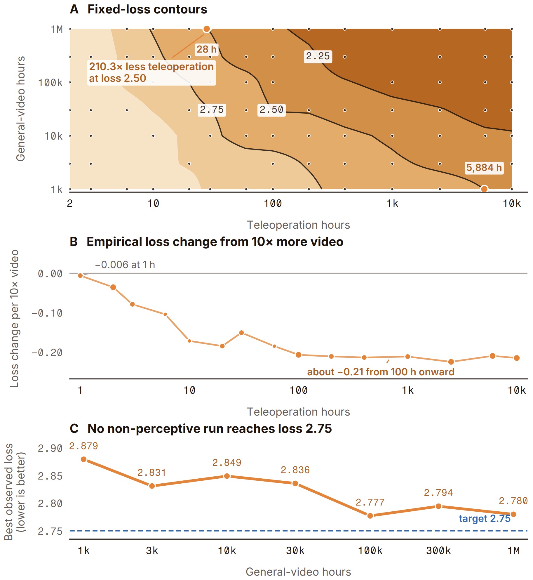
Implications for World-Model Scaling
-
The scaling result suggests that observation-rich data and action-rich data are complementary rather than interchangeable. General video provides broad coverage of objects, environments, and state changes; egocentric video emphasizes hands, contact, and interaction; UMI-style handheld data moves closer to manipulable trajectories; teleoperation supplies the embodiment-specific state-action mapping. Introducing Isaac 0.5 explicitly describes these data sources as progressively connecting visual knowledge to manipulation and finally to a complete action space.
-
A useful abstraction is therefore:
with each term supplying a different type of supervision rather than a homogeneous pool of trajectories.
- The key scaling interaction can be expressed qualitatively as:
where \(V\) is video scale and \(H_{\mathrm{teleop}}\) is action-grounded teleoperation scale. In the measured Isaac 0.5 regime, the magnitude of the video benefit grows sharply once enough action grounding is present. This differs from a naive assumption of separable scaling:
\[\mathcal{L}_{\mathrm{action}} \neq f(V) + g(H_{\mathrm{teleop}})\]because the empirical effect of additional video depends on the amount of robot control data available.
- This interaction provides a useful bridge between JEPA-style video pretraining and WAM-style video-action cotraining. V-JEPA 2 by Assran et al. (2025) shows that internet-scale video can learn a latent predictive representation that later supports action-conditioned planning; FLUX 3 Action shows that video and actions can be jointly generated within a generative WAM; Isaac 0.5 demonstrates a third route in which action-free video trains semantic future prediction inside the same backbone used for direct control.
Significance
-
Isaac 0.5 broadens the design space of predictive embodied models. Predictive control need not require explicit RGB future generation, and semantic future modeling need not be isolated in a separate planner. A shared model can use action-free video to learn future-oriented semantic state while exposing direct robot-action interfaces from the same representation.
-
The resulting continuum is:
- These categories are not mutually exclusive architectures but choices about which future variable is made explicit. Isaac 0.5 makes a semantic percept explicit; V-JEPA 2 makes a learned future representation explicit; FLUX 3 Action makes future video and action trajectories explicit. The common principle is that action improves when the representation is trained not only to recognize the present but also to encode task-relevant future change.
Representation Carriers in WAMs
Explicit, Geometric, and Latent Future Carriers
-
A central architectural question in World Action Models is what kind of future-state representation should mediate between perception, prediction, and action. A VLA normally represents the current scene and instruction only deeply enough to output an action, a WM represents the current state deeply enough to predict a future state under an action, and a WAM must represent future state in a form that is both predictive and action-decodable. RT-2: Vision-Language-Action Models Transfer Web Knowledge to Robotic Control by Brohan et al. (2023) represents actions as text-like tokens in a VLM-style policy, while World Action Models: The Next Frontier in Embodied AI by Wang et al. (2026) frames WAMs as models that couple future-state prediction with action generation.
-
The following figure (source) shows schematic cascaded WAM structures: a learned-action pipeline in which generated RGB futures are mapped to actions by an inverse-dynamics or action model, a geometric-extraction pipeline in which visual plans are converted into trajectories through geometric computation, and a latent-representation pipeline in which future latent states replace future RGB frames.
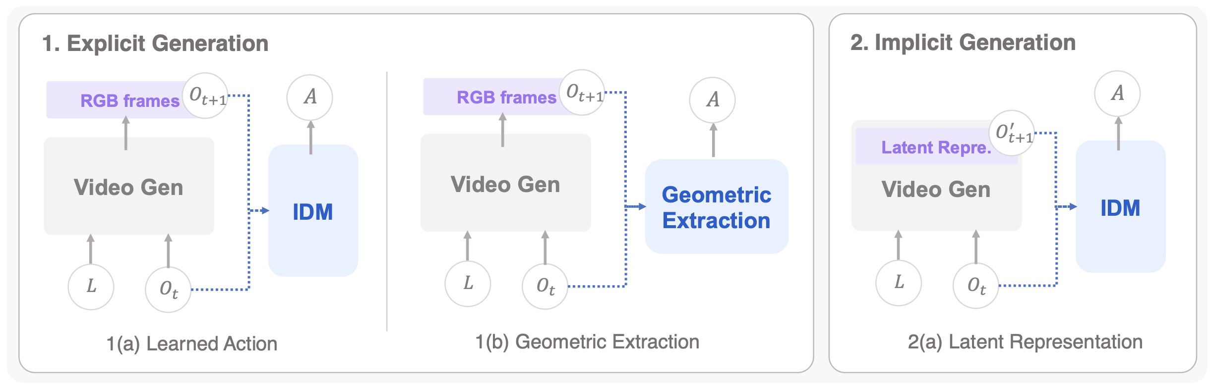
-
The most direct carrier is an explicit visual future, usually a video, keyframe sequence, image goal, or generated subgoal. In this case, the world-prediction stage can be written as:
\[\hat{o}_{t+1:t+H} \sim p_\theta(o_{t+1:t+H}\mid o_{\leq t},l)\]-
and the action decoder is trained or queried as:
\[\hat{a}_{t:t+H} \sim p_\phi(a_{t:t+H}\mid o_{\leq t},l,\hat{o}_{t+1:t+H})\]
-
-
This explicit representation is attractive because it is inspectable: humans, value models, VLMs, or downstream policies can evaluate whether the predicted future appears to satisfy the instruction. Learning Universal Policies via Text-Guided Video Generation by Du et al. (2023) casts sequential decision-making as text-conditioned video generation followed by action extraction, while Video Language Planning by Du et al. (2023) uses text-to-video dynamics models inside a tree-search procedure for long-horizon visual planning.
-
The limitation of explicit video carriers is that visual plausibility is not equivalent to action feasibility. A generated video may show the correct final configuration while hiding the contact forces, gripper constraints, occlusions, or intermediate robot motions needed to make that configuration physically reachable. This creates an inverse-dynamics ambiguity: many action sequences can correspond to similar frame transitions, and some visually plausible transitions may correspond to no feasible robot trajectory at all. Learning to Act from Actionless Videos through Dense Correspondences by Ko et al. (2023) addresses this gap by using dense correspondences to recover robot behavior from videos without action annotations, illustrating why the visual future alone is usually insufficient for control.
-
A second carrier is geometric structure, such as dense optical flow, point tracks, object poses, depth, surface normals, camera motion, or end-effector trajectories. This carrier can be written as:
\[g_{t+1:t+H} = G(\hat{o}_{t+1:t+H})\]-
where \(G\) extracts geometry or correspondence structure from the imagined future, followed by:
\[\hat{a}_{t:t+H} = \pi_\phi(o_{\leq t},l,g_{t+1:t+H})\]
-
-
Geometric carriers are more action-oriented than raw pixels because they expose motion, displacement, and spatial relations directly. They are especially useful when the action can be derived from pose changes, object tracks, or end-effector displacement. However, they remain brittle when the true control problem depends on hidden state, compliance, friction, force, tactile feedback, or deformable-object dynamics.
-
A third carrier is a latent future representation. Instead of reconstructing the full observation, the model predicts a compact state:
- The action model then conditions on this predicted latent future:
-
Latent carriers are often better matched to JEPA-style world modeling because they can discard high-entropy visual details while preserving predictable action-relevant structure. V-JEPA 2: Self-Supervised Video Models Enable Understanding, Prediction and Planning by Assran et al. (2025) pretrains a video JEPA on internet-scale video and then post-trains an action-conditioned latent world model for robot planning, while VLA-JEPA: Enhancing Vision-Language-Action Model with Latent World Model by Sun et al. (2026) uses leakage-free latent state prediction to make VLA pretraining focus on action-relevant dynamics rather than pixel-level nuisance variation.
-
The latent approach changes the learning target from observation likelihood to representation compatibility:
- When actions are available, the latent future can be made explicitly action-conditioned:
- For WAMs, this is not only a representation-learning objective. It also becomes a control interface: the predicted latent future must retain the variables that the action decoder needs, such as object pose, contact-relevant geometry, task progress, occluded object state, and affordance structure.
Semantic Prediction Between Pixels and Latents
-
JEPA-style prediction is not the only way to avoid reconstructing every future pixel. Isaac 0.5: Percepts Scale Control by Perceptron (2026) introduces future-percept prediction, where the target is semantic information automatically derived from a later observation, such as object state, affordance, contact change, task phase, or a likely near-future task state.
-
This adds a useful intermediate point to the representation spectrum:
-
A pixel model makes the target maximally observable but high entropy. A JEPA makes the target compact and learned, but potentially difficult to interpret. A semantic percept target attempts to expose the future variables most relevant to embodied reasoning while remaining grounded in visible state change. In Isaac 0.5, this prediction objective updates the same shared backbone used by the action interfaces, so semantic future prediction is not merely an auxiliary diagnostic.
-
The comparison also clarifies an important distinction with V-JEPA 2: Self-Supervised Video Models Enable Understanding, Prediction and Planning by Assran et al. (2025): V-JEPA 2 learns a generic predictive embedding from video and then trains an action-conditioned predictor for planning, whereas Isaac 0.5 cotrains semantic future prediction and direct robot control in one shared representation. The former emphasizes latent simulation and model-predictive control; the latter emphasizes transferable semantic foresight inside a direct policy.
Semantic Future Percepts
-
In addition to explicit visual futures, geometric futures, latent futures, and joint state-action streams, predictive embodied models can use semantic future percepts as the carrier between observation and control. Isaac 0.5: Percepts Scale Control by Perceptron (2026) defines a percept as a task-relevant visible state or change inferred from future observations rather than as a complete future frame or unconstrained hidden embedding.
-
A semantic carrier can be written abstractly as:
where \(p_{t+\Delta}\) may encode object state, relation, affordance, task phase, or visible contact change. Control then consumes a shared representation trained to support both the semantic future and action outputs:
\[\hat{a}_{t:t+K} = \pi_\phi \left( h_\theta(o_{\leq t},s_t,l) \right)\]-
This representation differs from an explicit visual carrier because it does not attempt to preserve texture, appearance, or every future pixel, and it differs from a generic latent carrier because the prediction target is semantically interpretable. It is especially attractive when task success depends on visible state transitions such as “drawer open,” “object grasped,” or “contact established,” while precise action execution can remain delegated to an action-specific decoder.
-
The carrier taxonomy can therefore be extended:
- Explicit visual futures preserve rich observation-level detail and human inspectability.
- Geometric futures expose spatial variables such as points, poses, depth, or trajectories.
- Semantic future percepts expose task-relevant visible states and changes without full rendering.
- Latent futures preserve compressed predictive structure without requiring semantic interpretability.
- Joint state-action streams model prediction and control together in a common autoregressive or generative trajectory.
-
Isaac 0.5 also shows that the carrier need not be the final policy output. The semantic future objective can operate as representation-shaping supervision while discrete FAST tokens and continuous Flow actions remain distinct interfaces. This creates a useful separation between the variable used to teach foresight and the variable used to execute control.
Joint State-Action Carriers
- A fourth carrier is a joint state-action token stream or shared diffusion trajectory. Instead of predicting a future first and decoding actions later, a joint WAM models future states and actions in one sequence:
- In an autoregressive model, the factorization is:
- This design allows state and action prediction to reinforce one another. The action tokens pressure the future-state representation to preserve controllable dynamics, while future-state tokens pressure the action representation to remain physically grounded. WorldVLA: Towards Autoregressive Action World Model by Cen et al. (2025) unifies future-image prediction and action generation in one autoregressive action-world model and reports mutual improvement between the world-model and action-model components.
Parallel Generative Carriers: FLUX 3 Action
-
FLUX 3 Action provides a concrete example of the shared-diffusion representation carrier. Rather than serializing future states and actions autoregressively, it represents future-video tokens and action tokens as separate but interacting streams inside the same generative process. A simplified joint state can be written as:
\[x_0 = \left[ v_{t+1:t+H}; a_{t:t+K} \right]\]- where \(v_{t+1:t+H}\) denotes latent future-video representations and \(a_{t:t+K}\) denotes the action trajectory. Both streams are corrupted and reconstructed within the same flow-matching model:
-
This design occupies an important middle ground between explicit visual carriers and purely latent carriers. Future video remains an explicit generative target, so the model retains pressure to represent observable world evolution, but actions are not extracted afterward by an independent inverse-dynamics model. Instead, visual futures and actions are generated jointly and can exchange information throughout denoising. FLUX 3 Action shows this directly by training a shared 7B backbone to predict future video and robot-control trajectories together.
-
Joint generation also means that the visual future does not necessarily need to be decoded into RGB during deployment. Video prediction can function as an internal training and inference constraint while the robot consumes only the action stream. This distinction is useful for WAMs because an explicit predictive target can shape the representation even when rendering every predicted frame would add unnecessary deployment latency.
-
FLUX 3 Action further shows that the carrier need not use identical noise statistics for all modalities. Video and actions differ strongly in dimensionality, entropy, and reconstruction difficulty, so the action representation is rescaled and the corruption schedule is tuned to control how quickly actionable information becomes recoverable relative to visual information. This extends the general WAM representation problem beyond deciding whether to use pixels or latents: a joint carrier must also decide how information from different modalities is temporally exposed during generation.
-
The representation-carrier taxonomy can therefore be refined to distinguish two forms of joint WAMs:
- Serialized joint carriers: future-state and action tokens are produced in a common autoregressive sequence, allowing earlier predictions to causally condition later ones. WorldVLA: Towards Autoregressive Action World Model by Cen et al. (2025) is an example of this formulation.
- Parallel generative carriers: future-state and action representations are refined together through diffusion or flow matching, enabling bidirectional interaction during generation rather than imposing a fixed left-to-right ordering. FLUX 3 Action is a concrete example of this formulation.
-
This makes the choice of representation carrier inseparable from the generative mechanism. Autoregressive WAMs impose an explicit causal ordering between state and action tokens, while diffusion- and flow-based WAMs can iteratively refine both representations together.
Choosing the Representation Carrier
-
The representation carrier should therefore be selected according to the failure mode that matters most:
- Explicit visual futures: best when interpretability, subgoal visualization, or video-pretrained priors are central, but weak when action feasibility depends on hidden physical state.
- Geometric futures: best when object motion, point motion, depth, or pose can be converted into control, but weak when geometry extraction is noisy or contact dynamics dominate.
- Latent futures: best when compactness, robustness, and action-relevant abstraction matter more than human inspection, but weak when the latent state is hard to audit.
- Joint state-action streams: best when the model should co-train prediction and control end-to-end, but weak when debugging requires a clean separation between the world model and policy.
-
A useful WAM representation objective combines these pressures:
\[\mathcal{L}_{\mathrm{rep\text{-}WAM}} = \lambda_f d(\hat{y}_{t+1:t+H},y_{t+1:t+H}) + \lambda_a \ell(\hat{a}_{t:t+H},a_{t:t+H}) + \lambda_c \sum_{k=0}^{H-1} d\left( T(\hat{y}_{t+k},\hat{a}_{t+k}), \hat{y}_{t+k+1} \right)\]- where \(y\) may denote pixels, geometry, or latent states; \(d\) is the appropriate distance or likelihood loss; \(\ell\) is the action loss; and \(T\) is a learned or analytic transition consistency operator. The key design principle is that a WAM representation is not merely a compressed observation. It is a future-facing control variable that must be predictable, physically meaningful, and decodable into executable action.
Temporal Horizons
Action Horizons in VLAs
-
Temporal abstraction is one of the clearest axes along which Vision-Language-Action models, World Action Models, and World Models differ. A VLA usually abstracts time into an action horizon: given the current observation and instruction, it predicts the next action or an action chunk. A WM abstracts time into a dynamics horizon: given the current state and candidate actions, it predicts future states. A WAM must align both horizons: it predicts actions and future states over compatible time windows so that the action sequence is constrained by an anticipated physical trajectory. RT-1: Robotics Transformer for Real-World Control at Scale by Brohan et al. (2022) introduced a scalable transformer policy for real-world robot control, while World Action Models: The Next Frontier in Embodied AI by Wang et al. (2026) defines WAMs as embodied models that jointly predict future states and actions rather than actions alone.
-
For a VLA, the temporal problem is primarily policy smoothing and short-horizon action coherence:
\[a_{t:t+K} \sim p_\theta(a_{t:t+K}\mid o_{\leq t},l)\]-
where \(K\) is the action-chunk horizon. The objective is:
\[\mathcal{L}_{\mathrm{VLA\text{-}chunk}} = \mathbb{E} \left[ -\log p_\theta(a_{t:t+K}\mid o_{\leq t},l) \right]\]
-
-
This formulation is useful because robot control is temporally correlated: a grasp, insertion, wipe, or drawer-opening motion is not a single isolated command but a locally coherent sequence. Learning Fine-Grained Bimanual Manipulation with Low-Cost Hardware by Zhao et al. (2023) introduces Action Chunking with Transformers to predict short action sequences and reduce compounding error in imitation learning, while Diffusion Policy: Visuomotor Policy Learning via Action Diffusion by Chi et al. (2023) represents visuomotor control as conditional denoising over action trajectories and uses receding-horizon execution.
Prediction Horizons in World Models
- For a WM, the temporal problem is forward rollout stability:
- A multi-step latent rollout objective can be written as:
-
The key challenge is compounding prediction error: even small one-step errors can accumulate over long rollouts, causing the predicted latent state to drift away from states that are physically reachable or useful for planning. Learning Latent Dynamics for Planning from Pixels by Hafner et al. (2019) uses learned latent dynamics for online planning from image observations, and Dream to Control: Learning Behaviors by Latent Imagination by Hafner et al. (2019) trains policies from imagined latent rollouts, making rollout stability central to model-based control.
-
Semantic future prediction introduces a related but distinct temporal abstraction: the prediction offset \(\Delta\) need not correspond to an explicitly rendered rollout of length \(H\). Isaac 0.5: Percepts Scale Control by Perceptron (2026) predicts a task-relevant percept derived from a later observation at \(t+\Delta\), allowing the representation to encode that a drawer should be open, an object should be grasped, or contact should occur without requiring the model to reconstruct every intervening visual state. The temporal variables therefore serve different roles:
\[\Delta = \text{semantic prediction offset}, \qquad H = \text{explicit world-model rollout horizon}, \qquad K = \text{action horizon}\] -
A semantic prediction target can consequently supervise relatively long-range task progress while leaving the detailed intermediate trajectory implicit. This can reduce the burden of long video rollouts, but it also means that predicting a correct future percept does not by itself establish that every intermediate state is dynamically reachable. Explicit WMs and WAMs retain an advantage when control requires reasoning about the complete path between the current state and the predicted outcome.
Coupled Horizons in World Action Models
- For a WAM, the temporal problem is action-future alignment across two horizons:
-
The prediction horizon \(H\) and action horizon \(K\) need not be identical, but they must be compatible. A short action chunk may only realize the first step of a longer imagined future, while a long action chunk may require intermediate future states to remain feasible. A WAM objective can therefore include a temporal alignment loss:
\[\mathcal{L}_{\mathrm{temporal\text{-}align}} = \sum_{k=0}^{\min(H,K)-1} d\left( T(\hat{z}_{t+k},\hat{a}_{t+k}), \hat{z}_{t+k+1} \right)\]- where \(T\) is a learned or analytic transition operator and \(d\) is a state-space distance or negative log-likelihood. This term pressures the generated action trajectory and generated future trajectory to agree at every intermediate step, not only at the final goal.
-
The temporal difference between the three families can be summarized as:
- VLA: the model predicts temporally coherent control, but future-state prediction is not required.
- WM: the model predicts temporally coherent state evolution, but action generation is not required.
- WAM: the model predicts temporally coherent state evolution and temporally coherent control, while enforcing agreement between the two.
-
This distinction matters most when long-horizon behavior requires intermediate physical foresight. In a simple reaching task, a VLA may succeed by mapping the object location directly to a motion primitive. In a long-horizon manipulation task, such as opening a drawer, retrieving an object, and placing it into a container, the agent must preserve task progress over multiple state transitions. A WM can simulate possible futures, but a WAM can bind those futures to executable action chunks, making it better suited to language-conditioned manipulation where the correct action depends on the anticipated consequence rather than the current image alone.
Autoregressive and Diffusion-Based Temporal Modeling
- Autoregressive WAMs expose the temporal trade-off most clearly. If future observations and actions are serialized into one sequence, the model can factorize prediction as:
-
This gives strong causal structure, because earlier predicted futures can condition later predicted actions. The cost is sequential latency and error propagation: an early hallucinated future state can corrupt later action predictions. WorldVLA: Towards Autoregressive Action World Model by Cen et al. (2025) explicitly reports that autoregressive action generation can degrade across action sequences and proposes an attention-mask strategy to reduce harmful dependence on earlier predicted actions.
-
Diffusion and flow-based WAMs expose the complementary trade-off. Instead of producing tokens left-to-right, they denoise a trajectory in parallel:
\[x_\tau = \alpha_\tau x_0+\sigma_\tau \epsilon, \qquad \epsilon\sim\mathcal{N}(0,I),\]-
where \(x_0\) may contain future latent states, future observations, action chunks, or a shared state-action trajectory. The denoising objective is commonly written as:
\[\mathcal{L}_{\mathrm{diff}} = \mathbb{E}_{x_0,\epsilon,\tau} \left[ \left\| \epsilon - \epsilon_\theta(x_\tau,\tau,o_{\leq t},l) \right\|_2^2 \right]\]
-
-
This improves multimodal trajectory modeling and parallel refinement, but it can make causal ordering less explicit than autoregressive decoding. Diffusion Policy by Chi et al. (2023) demonstrates the strength of action diffusion for multimodal visuomotor control, while Video Prediction Policy: A Generalist Robot Policy with Predictive Visual Representations by Hu et al. (2024) conditions robot policies on predictive visual representations learned from video diffusion models.
Receding-Horizon Predictive Execution
- A practical WAM can combine these ideas through receding-horizon predictive execution. At time \(t\), the model predicts a future-state trajectory and action chunk:
-
Only the first action or first few actions are executed:
\[a_t = \hat{a}_t\]- then the model observes the new state and replans. This reduces exposure to long-horizon prediction errors while preserving the benefit of physical foresight. V-JEPA 2: Self-Supervised Video Models Enable Understanding, Prediction and Planning by Assran et al. (2025) follows this broad principle by post-training an action-conditioned latent world model and using planning in representation space for robot manipulation.
Prediction, Action, and Commit Horizons
- FLUX 3 Action provides a concrete example of how a WAM can separate its prediction horizon from its execution horizon. Its DROID configuration predicts 32 actions at a control frequency of 15 Hz, giving a nominal full action-chunk horizon of:
- The full predicted chunk need not be executed open-loop. Instead, the controller can execute a prefix of the predicted trajectory, observe the resulting world state, and run the WAM again:
-
This creates three distinct temporal quantities that should not be conflated:
\[T_{\mathrm{prediction}} \geq T_{\mathrm{action\ chunk}} \geq T_{\mathrm{execution}}\]- where \(T_{\mathrm{prediction}}\) is how far the internal future model looks ahead, \(T_{\mathrm{action\ chunk}}\) is how much control the model predicts in one invocation, and \(T_{\mathrm{execution}}\) is how much of that prediction is actually committed before observing the environment again.
-
The distinction is important when comparing WAMs with conventional VLAs. In BFL’s reported configuration, FLUX 3 Action produces approximately \(2.13\) seconds of action trajectory per prediction, whereas \(\pi_0.5\): A Vision-Language-Action Model with Open-World Generalization predicts approximately \(1\) second under the comparison setup. A longer generated action horizon can improve effective real-time throughput even when raw model-call latency is similar, because each inference invocation supplies more potential robot motion.
-
However, a longer predicted chunk should not automatically imply a longer open-loop execution interval. The value of a WAM is precisely that prediction can extend farther into the future than the amount of action the robot is willing to execute without feedback. This separates physical foresight from control commitment: the model can reason over a multi-second future while still replanning frequently enough to respond to failed grasps, moved objects, contact errors, or observation changes.
-
The temporal design problem for WAMs is therefore better expressed using three coupled horizons rather than two:
- World horizon \(H\): how far future observations or latent states are predicted.
- Action horizon \(K\): how many future controls are generated together.
- Commit horizon \(C\): how many generated actions are executed before replanning, with \(C \leq K\).
-
A closed-loop WAM can then be written as:
\[(\hat{z}_{t+1:t+H}, \hat{a}_{t:t+K}) \sim p_\theta\left( z_{t+1:t+H}, a_{t:t+K} \mid z_{\leq t}, l \right)\]- followed by:
- before refreshing the observation and repeating the prediction-control cycle.
-
This three-horizon formulation makes clear why longer action chunks and world predictions need not reduce feedback frequency. Predictive depth and closed-loop responsiveness can be independently controlled.
-
The important design rule is that the temporal horizon should match the control bottleneck. Short horizons are appropriate for reflexive skills, contact-rich stabilization, and high-frequency servoing. Medium horizons are appropriate for manipulation primitives such as grasping, pouring, opening, placing, and pushing. Long horizons are appropriate for task planning, subgoal discovery, and instruction decomposition, but they require stronger state abstraction and uncertainty handling. A VLA mainly chooses the action horizon, a WM mainly chooses the prediction horizon, and a WAM must choose both jointly so that predicted futures remain actionable and predicted actions remain physically grounded.
Uncertainty, Belief States, and Risk
- Partial observability is central to embodied intelligence because the current observation rarely exposes the complete world state. Objects may be occluded, contact forces may be hidden, robot proprioception may be noisy, humans may act unpredictably, and visual appearance may not reveal material properties such as mass, friction, compliance, or containment. A belief state summarizes this hidden information as a distribution rather than a point estimate:
-
A VLA usually handles this uncertainty implicitly. It maps the observation history and instruction to an action distribution:
\[p_\theta(a_t \mid o_{\leq t}, l)\]- but it does not need to maintain an explicit posterior over hidden states. This means the model can express action uncertainty, for example by assigning probability mass to multiple possible actions, but it does not necessarily know whether uncertainty comes from visual ambiguity, missing state, stochastic dynamics, or policy indecision. RT-2: Vision-Language-Action Models Transfer Web Knowledge to Robotic Control by Brohan et al. (2023) demonstrates the strength of VLA-style action prediction through tokenized robot actions, while OpenVLA: An Open-Source Vision-Language-Action Model by Kim et al. (2024) scales this formulation as an open generalist robot policy.
-
A WM treats uncertainty as part of the dynamics model. Instead of predicting a single future state, it models a conditional distribution \(p_\phi(z_{t+1} \mid z_t, a_t)\) or under partial observability \(p_\phi(z_{t+1} \mid b_t, a_t)\).
-
A Bayesian filtering update can be written as:
\[b_{t+1}(z_{t+1}) \propto p(o_{t+1}\mid z_{t+1}) \int p(z_{t+1}\mid z_t,a_t) b_t(z_t) \,dz_t\] -
This is the classical world-model advantage: uncertainty is attached to the latent state and propagated forward under hypothetical actions. PETS: Deep Reinforcement Learning in a Handful of Trials using Probabilistic Dynamics Models by Chua et al. (2018) makes this operational through probabilistic ensembles with trajectory sampling, allowing model predictive control to reason over uncertainty-aware rollouts rather than a single deterministic trajectory.
-
A WAM must represent uncertainty over both futures and actions:
-
This is a stronger requirement than either a VLA or a WM alone. A VLA may be uncertain about which action to take; a WM may be uncertain about which future will occur after an action; a WAM must model whether a particular action sequence and a particular future trajectory are jointly compatible. World Action Models: The Next Frontier in Embodied AI by Wang et al. (2026) defines WAMs as embodied models that unify predictive state modeling with action generation by targeting a joint distribution over future states and actions.
-
In a cascaded WAM, uncertainty can be represented by sampling multiple possible futures:
\[\hat{z}_{t+1:t+H}^{(i)} \sim p_\theta(z_{t+1:t+H}\mid b_t,l), \qquad i=1,\dots,N\]-
then decoding or selecting actions conditioned on those futures:
\[\hat{a}_{t:t+K}^{(i)} \sim p_\phi(a_{t:t+K}\mid b_t,l,\hat{z}_{t+1:t+H}^{(i)})\]
-
-
This makes uncertainty interpretable because the system can inspect alternative imagined outcomes before acting. The weakness is interface mismatch: the future generator may assign high probability to futures that the action decoder cannot realize, or the action decoder may ignore uncertainty in the imagined future.
-
In a joint WAM, uncertainty is modeled inside a shared state-action distribution:
-
This can reduce mismatch because future prediction and action prediction are coupled during training. The trade-off is that uncertainty may become harder to audit if it is stored in latent tokens, diffusion trajectories, or implicit hidden states rather than explicit visual rollouts. VLA-JEPA: Enhancing Vision-Language-Action Model with Latent World Model by Sun et al. (2026) represents this latent-predictive direction by using future-state prediction to improve VLA pretraining, while V-JEPA 2: Self-Supervised Video Models Enable Understanding, Prediction and Planning by Assran et al. (2025) post-trains an action-conditioned latent world model for robot planning after internet-scale video pretraining.
-
Semantic future prediction introduces a similar uncertainty problem. A compact percept can deliberately discard nuisance visual detail, but the same compression may also hide ambiguity about which future state will occur. Instead of producing only a point prediction \(\hat{p}_{t+\Delta}\), a risk-aware semantic predictor should ideally represent a calibrated distribution:
\[p_\theta \left( p_{t+\Delta} \mid o_{\leq t} \right)\]- so that uncertainty over mutually plausible task states remains visible to the controller. This is particularly important when multiple semantic outcomes are compatible with the same observation history, such as uncertain grasp success, ambiguous contact, partial occlusion, or several plausible task phases.
-
Semantic abstraction therefore trades observation-level detail for task relevance, but it should not collapse epistemic or multimodal uncertainty along with that detail. Isaac 0.5: Percepts Scale Control by Perceptron (2026) defines the percept target and its role in the shared control representation, while leaving the target-construction and loss implementation proprietary; uncertainty calibration over these semantic futures therefore remains an important open design question rather than a disclosed property of the system.
-
Risk-sensitive WAMs should not choose the action with the best average predicted outcome if that action has catastrophic low-probability failures. A risk-aware objective can augment expected cost with uncertainty penalties:
-
One common risk functional is conditional value at risk:
\[\operatorname{CVaR}_{\alpha}(C) = \mathbb{E} \left[ C \mid C \geq q_{\alpha}(C) \right]\]- where \(q_{\alpha}(C)\) is the \(\alpha\)-quantile of the cost distribution. In manipulation, this matters because a low-average-cost action may still have unacceptable tail risk, such as dropping a fragile object, colliding with a person, or forcing an insertion under uncertain contact geometry.
-
JEPA-style world models are particularly relevant because standard deterministic JEPA objectives predict a point estimate in representation space, while probabilistic JEPA variants make uncertainty explicit. A schematic probabilistic JEPA objective can be written as:
\[\mathcal{L}_{\mathrm{VJEPA}} = \mathbb{E}_{q_\phi(\xi \mid h_t,z_{t+1})} \left[ \left\| g_\theta(h_t,\xi)-z_{t+1} \right\|_2^2 \right] + \beta D_{\mathrm{KL}} \left( q_\phi(\xi \mid h_t,z_{t+1}) \parallel p_\eta(\xi\mid h_t) \right)\]- where \(h_t\) is the context representation and \(\xi\) is a latent stochastic variable. VJEPA: Variational Joint Embedding Predictive Architectures as Probabilistic World Models by Huang (2026) extends JEPA into a probabilistic predictive framework by learning distributions over future latent states, connecting JEPA-style representation learning to predictive state representations and Bayesian filtering.
-
For WAMs, uncertainty should also be consistency-aware. It is not enough for the future distribution to be broad or calibrated independently of the action distribution. The model should assign high probability only to futures that are reachable under the predicted actions. A consistency-aware uncertainty term can be written as:
\[\mathcal{L}_{\mathrm{uncertain\text{-}consistency}} = \mathbb{E}_{(\hat{z},\hat{a})\sim p_\psi} \left[ \sum_{k=0}^{H-1} d\left( T(\hat{z}_{t+k},\hat{a}_{t+k}), \hat{z}_{t+k+1} \right) \right]\]- where \(T\) is a learned or analytic transition operator. This term penalizes futures that are plausible in isolation but not reachable through the model’s own predicted control sequence.
-
The evaluation implication is straightforward: uncertainty must be measured jointly across perception, dynamics, and control. VLAs need calibrated action confidence, especially under distribution shift. WMs need calibrated transition uncertainty and stable multi-step rollouts. WAMs need calibrated state-action uncertainty, meaning that predicted futures, predicted actions, and realized outcomes should agree. World Action Models: The Next Frontier in Embodied AI by Wang et al. (2026) organizes WAM evaluation around visual fidelity, physical commonsense, and action plausibility, which matches the requirement that uncertainty be assessed not only by how realistic futures look, but by whether they support physically executable actions.
Data and Evaluation
-
Training data determines whether a model learns semantic action imitation, physical prediction, or prediction-grounded control. A VLA is primarily shaped by paired robot demonstrations, a WM is shaped by transition data, and a WAM requires both future-state supervision and action supervision, either in the same trajectory or through a staged training recipe that combines large-scale video with smaller amounts of robot interaction data. World Action Models: The Next Frontier in Embodied AI by Wang et al. (2026) organizes the WAM data ecosystem around robot teleoperation, portable human demonstrations, simulation, and internet-scale egocentric video, which is a useful way to separate action-rich data from observation-rich data.
-
The following figure (source) shows a schematic overview of world models for VLA learning and evaluation. World models can support imitation learning by generating or filtering training trajectories, reinforcement learning by enabling imagined interaction and reward-guided policy optimization, reward modeling by producing reward signals from learned dynamics or future outcomes, and policy evaluation by serving as data-driven simulators for virtual rollout and testing, where \(\mathcal{T}\) denotes rollout trajectories.
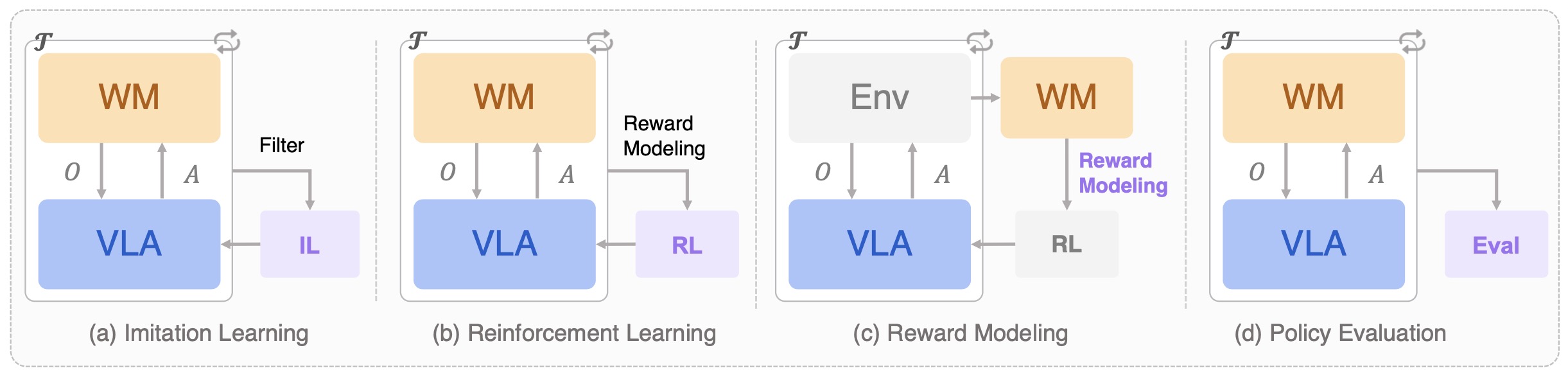
- A VLA training set usually consists of language-conditioned demonstrations:
- A WM training set consists of action-conditioned transitions:
- A WAM training set ideally contains instruction, observation history, future states, and executable actions:
-
This difference explains why WAMs are harder to scale than either VLAs or WMs alone. Robot demonstrations contain actions but are expensive, embodiment-specific, and limited in diversity. Internet video contains enormous visual and temporal diversity but usually lacks robot action labels. Simulation can generate state-action trajectories cheaply but may suffer from sim-to-real gaps. Portable human-demonstration systems sit between these extremes by collecting task-rich manipulation behavior outside fixed robot labs. Open X-Embodiment: Robotic Learning Datasets and RT-X Models by O’Neill et al. (2023) aggregates robot data from 22 embodiments and reports positive transfer across platforms, DROID: A Large-Scale In-The-Wild Robot Manipulation Dataset by Khazatsky et al. (2024) provides 76K real-world manipulation trajectories across 564 scenes and 84 tasks, and Universal Manipulation Interface: In-The-Wild Robot Teaching Without In-The-Wild Robots by Chi et al. (2024) uses handheld grippers to collect portable human demonstrations for deployable robot policies.
-
A scalable WAM recipe can combine these data sources through a mixture objective:
\[\mathcal{L} = \lambda_{\mathrm{act}}\mathcal{L}_{\mathrm{act}} + \lambda_{\mathrm{future}}\mathcal{L}_{\mathrm{future}} + \lambda_{\mathrm{align}}\mathcal{L}_{\mathrm{align}} + \lambda_{\mathrm{sim}}\mathcal{L}_{\mathrm{sim}}\]- Here, \(\mathcal{L}_{\mathrm{act}}\) trains action prediction on robot demonstrations, \(\mathcal{L}_{\mathrm{future}}\) trains future prediction on videos or transitions, \(\mathcal{L}_{\mathrm{align}}\) binds predicted futures to executable actions, and \(\mathcal{L}_{\mathrm{sim}}\) regularizes behavior in synthetic environments. This mixture is useful because WAMs need semantic diversity from web-scale visual data, physical diversity from human and egocentric video, and embodiment grounding from robot trajectories. Ego4D: Around the World in 3,000 Hours of Egocentric Video by Grauman et al. (2022) provides large-scale egocentric video for first-person perception, while V-JEPA 2: Self-Supervised Video Models Enable Understanding, Prediction and Planning by Assran et al. (2025) shows how internet-scale action-free video pretraining can be paired with a much smaller amount of robot trajectory data to support latent planning.
-
Observation-rich and action-rich datasets should not be treated as independently additive components of a training mixture. Isaac 0.5: Percepts Scale Control by Perceptron (2026) finds a strong interaction between video scale and teleoperation scale: additional action-free video has little effect when action grounding is extremely sparse, but its contribution becomes substantially larger once sufficient robot supervision is present. A more appropriate abstraction is therefore:
\[\mathcal{L}_{\mathrm{action}} = F \left( H_{\mathrm{video}}, H_{\mathrm{teleop}} \right)\]-
rather than assuming a separable relationship of the form:
\[\mathcal{L}_{\mathrm{action}} = f(H_{\mathrm{video}}) + g(H_{\mathrm{teleop}})\]
-
-
This interaction also changes how headline data-efficiency ratios should be interpreted. The reported \(210.3\times\) reduction in teleoperation at a fixed offline action-loss threshold is a within-grid exchange rate for one particular recipe, not a universal conversion factor between video hours and robot hours. At one hour of teleoperation, a \(10\times\) increase in video changes held-out action loss by only about \(-0.006\), whereas from roughly 100 teleoperation hours onward the same multiplicative increase produces an improvement near \(-0.21\). The more general lesson is therefore that broad video priors become most useful after the representation has been sufficiently grounded in an executable action space.
Video-Robot Data Exchange Rates
- The usual distinction between observation-rich and action-rich data can be made quantitative. Isaac 0.5: Percepts Scale Control by Perceptron (2026) varies a fixed-ratio mixture of general, egocentric, and UMI video against teleoperation and evaluates held-out robot action loss, producing an empirical surface:
-
At the reported action-loss threshold \(\tau=2.50\), scaling general video from \(10^3\) to \(10^6\) hours moves the interpolated teleoperation crossing from \(5{,}884\) hours to \(28\) hours, a \(210.3\times\) reduction within the measured grid. The adjacent measured teleoperation rungs bound the endpoint exchange ratio at approximately \(83\times\) to \(300\times\).
-
This result is conditional rather than a constant substitution rate. Video contributes little with only one hour of teleoperation, where a \(10\times\) video increase changes loss by roughly \(-0.006\), while the same multiplicative increase improves loss by approximately \(-0.21\) from around 100 teleoperation hours onward. The evaluation therefore supports a complementarity hypothesis:
\[\frac{\partial^2 \mathcal{L}_{\mathrm{action}}} {\partial \log H_{\mathrm{video}} \partial \log H_{\mathrm{teleop}}} \neq 0\]- meaning that the value of observation-only data depends on how well the model has already been grounded in actions.
-
This has an important implication for world-model evaluation. A predictive objective should not be judged only by whether it improves future-state accuracy or video understanding; it should also be evaluated by how strongly it changes downstream action-data efficiency. Isaac 0.5’s non-perceptive comparison runs remain above an action loss of \(2.75\) over the tested video budgets, which supports the narrower conclusion that, in the reported recipe, video scale alone does not produce the same action-loss frontier without the predictive percept objective.
Multi-Axis Evaluation
-
Isaac 0.5 also motivates evaluating one checkpoint across perception, reasoning, offline control prediction, adaptation, and physical execution rather than reporting only task success. Introducing Isaac 0.5 reports evaluations spanning multimodal video understanding, spatial grounding, held-out action prediction, benchmark-specific adaptation, and closed-loop robot control.
-
For predictive embodied models, evaluation should therefore include at least four linked axes:
- Predictive representation quality: whether future-oriented supervision improves semantic or latent state prediction.
- Action quality: whether the resulting representation lowers action prediction error and improves closed-loop success.
- Data efficiency: how much additional observation-rich data reduces the amount of embodiment-specific action supervision required.
- Cross-embodiment transfer: whether a common predictive representation can support multiple robot interfaces after configuration or lightweight adaptation.
-
This complements WAM metrics such as future quality and action-future agreement. A model like FLUX 3 Action exposes the predicted future directly and can be tested for consistency between generated futures and actions; a semantic predictive model such as Isaac 0.5 instead requires probing whether future-oriented semantic supervision changes action efficiency and transfer, because its predicted future need not be rendered as a complete video.
Evaluation Contracts
-
Evaluation should follow the same contract. A VLA is evaluated by task success, language grounding, generalization, action smoothness, and embodiment transfer. A WM is evaluated by predictive accuracy, temporal stability, physical plausibility, uncertainty calibration, and utility for planning. A WAM must be evaluated jointly: the future should be plausible, the action should be executable, and the action should causally explain the predicted future. This motivates a compatibility score such as:
\[S_{\mathrm{WAM}} = S_{\mathrm{task}} - \alpha d_{\mathrm{future}}(\hat{o}_{t+1:t+H},o_{t+1:t+H}) - \beta d_{\mathrm{dyn}}\left(T(\hat{z}_{t:t+H},\hat{a}_{t:t+K}),\hat{z}_{t+1:t+H}\right) - \gamma R_{\mathrm{safety}}\]- where \(S_{\mathrm{task}}\) measures task completion, \(d_{\mathrm{future}}\) measures future-state error, \(d_{\mathrm{dyn}}\) measures action-future consistency, and \(R_{\mathrm{safety}}\) penalizes unsafe or high-risk rollouts.
Benchmarking Predictive Embodied Models
-
Video and world-model benchmarks are useful but incomplete for WAMs because they often score generated futures separately from action execution. VBench-2.0: Advancing Video Generation Benchmark Suite for Intrinsic Faithfulness by Zheng et al. (2025) extends video evaluation beyond surface quality toward physics and commonsense, while WorldModelBench: Judging Video Generation Models As World Models by Li et al. (2025) evaluates world-modeling capabilities through commonsense, instruction following, and physics adherence.
-
Robot-policy benchmarks are also necessary but incomplete because task success alone may not reveal whether the model used predictive physical reasoning or dataset shortcuts. LIBERO: Benchmarking Knowledge Transfer for Lifelong Robot Learning by Liu et al. (2023) studies procedural and declarative transfer across robot manipulation suites, while Evaluating Real-World Robot Manipulation Policies in Simulation by Li et al. (2024) introduces SIMPLER to correlate simulated manipulation evaluation with real-world policy behavior.
RoboLab, Real-Robot Validation, and RoboArena
-
RoboLab: A High-Fidelity Simulation Benchmark for Analysis of Task Generalist Policies by Yang et al. (2026) provides a useful intermediate evaluation regime for WAMs because it runs policies trained on real-world data inside a standardized simulation environment rather than evaluating only offline action prediction or generated-video fidelity. RoboLab contains 120 manipulation tasks and varies language specificity, task complexity, and competency dimensions, allowing predictive policies and conventional VLAs to be compared under the same execution environment.
-
FLUX 3 Action achieved a 42.92% overall RoboLab-120 success rate in its reported evaluation, compared with 36.8% for Cosmos3-Nano-Policy, 28.0% for \(\pi_0.5\), 25.7% for DreamZero, and 7.2% for GR00T N1.6 in BFL’s comparison. These results are consistent with the hypothesis that explicit world-action prediction can improve embodied control, but they should not be interpreted as proving that WAMs universally dominate VLAs: architecture, parameter count, training data, embodiment interfaces, and inference compute differ across systems.
-
Leaderboard rank is also a weak long-term scientific descriptor because RoboLab is explicitly designed as an evolving benchmark. New policies and tasks can change relative positions without changing an existing model. Absolute success rate, task distribution, evaluation date, and evaluation protocol are therefore more useful than statements that a particular policy is permanently the benchmark leader. The live RoboLab leaderboard should be interpreted as a moving snapshot of the field rather than a fixed model property.
-
Simulation results should also be paired with physical-robot evaluation. FLUX 3 Action reports a blinded comparison conducted by Positronic Robotics in which a Franka arm attempted ten DROID-style single-object tasks three times each. FLUX 3 Action completed 28 of 30 attempts, compared with 27 for Cosmos 3 Nano, 20 for DreamZero, and 13 for \(\pi_0.5\). FLUX 3 Action uses this experiment as evidence that its simulated performance transfers to physical manipulation, although the small task and trial counts make it complementary to, rather than a replacement for, larger real-world benchmarks.
-
RoboArena: Distributed Real-World Evaluation of Generalist Robot Policies by Atreya et al. (2025) provides the stronger long-term evaluation model by comparing policies through distributed real-robot experiments and blind pairwise judgments. This matters for WAMs because simulation can reproduce object poses and task logic more easily than friction, compliance, sensing noise, actuator variation, hardware wear, clutter, and contact dynamics.
What a Mature WAM Benchmark Should Measure
-
A mature WAM benchmark should therefore report three quantities together:
- Future quality: whether the generated or latent future is visually, physically, and temporally plausible.
- Action quality: whether the predicted action sequence succeeds under real or high-fidelity simulated execution.
- Action-future agreement: whether the predicted action is the cause of the predicted future, rather than a parallel output that happens to look plausible.
Deployment Efficiency
-
FLUX 3 Action also highlights a fourth deployment-facing axis that should be reported separately from model quality: computational efficiency. WAMs may predict substantially more tokens than action-only policies because future video or latent-state streams remain active during inference. Evaluation should therefore report not only task success but also processing latency, generated action horizon, memory use, and control-time coverage per invocation. FLUX 3 Action reports a 32-action DROID configuration spanning approximately \(2.13\) seconds of motion per prediction, illustrating why per-call latency alone can be misleading when comparing robot policies.
-
A useful deployment metric is therefore the ratio between generated control time and inference time:
where larger values indicate that the policy can generate a longer executable horizon relative to its computation time. This metric should not replace success rate or action-future consistency, but it captures whether a computationally expensive WAM can practically sustain real-time closed-loop control.
- WAM evaluation should therefore be treated as a hierarchy rather than as a single benchmark score:
- A model can perform well at an earlier stage while failing at a later one. High-quality future videos do not guarantee executable actions, simulator success does not guarantee real-world robustness, and high task success may still be impractical if inference cannot keep pace with the control loop.
Open Challenges for Prediction-Grounded Embodied Models
-
The central open problem is not simply scaling VLAs, improving video generation, or building larger robot datasets. The central problem is coupling prediction and action so that an embodied model can use imagined consequences as a control variable. A VLA without explicit prediction may remain reactive, a WM without action generation may remain only a simulator, and a WAM without consistency constraints may generate futures and actions that are individually plausible but mutually incoherent. World Action Models: The Next Frontier in Embodied AI by Wang et al. (2026) identifies architectural coupling, multimodal physical state representation, evaluation, and reliable deployment as core challenges for the next phase of WAM research.
-
Architectural coupling: Cascaded WAMs are easier to inspect because the predicted future can be visualized, ranked, or edited before action decoding. Joint WAMs may be more efficient and better optimized end-to-end because future prediction and action generation share a representation. The unresolved question is when explicit future prediction is actually needed at inference time, and when it is mainly useful as an auxiliary training signal. A useful controlled comparison would match data, scale, action space, and benchmark conditions across:
-
This would separate the benefit of visual imagination, latent dynamics, auxiliary prediction gradients, and joint state-action decoding.
-
Multimodal physical state: Much of the information needed for manipulation is not visible in RGB. Contact force, friction, torque, compliance, slippage, acoustic feedback, tactile distributions, and proprioceptive uncertainty often determine whether a manipulation succeeds. A WAM that predicts only future pixels may miss the very variables that make an action safe or feasible. A richer state prediction target can be written as:
\[s_t = (o_t^{\mathrm{rgb}}, o_t^{\mathrm{depth}}, q_t^{\mathrm{robot}}, \tau_t^{\mathrm{force}}, h_t^{\mathrm{tactile}}, m_t^{\mathrm{material}})\]-
with a multimodal predictive objective:
\[\mathcal{L}_{\mathrm{multi}} = \sum_{m\in\mathcal{M}} \lambda_m d_m(\hat{s}_{t+1}^{(m)},s_{t+1}^{(m)})\]
-
-
The important shift is that the “world” in a World Action Model should not be equated with a video frame. It should be the set of latent and observable physical variables needed to choose safe, effective actions.
-
Causal grounding rather than visual correlation: A WAM must learn that actions intervene on the world, not merely co-occur with visual changes. This requires distinguishing observational prediction \(p(o_{t+1}\mid o_t,l)\) from intervention-conditioned prediction \(p(o_{t+1}\mid o_t,\operatorname{do}(a_t),l)\).
-
The second expression is the one that matters for control. Without intervention grounding, a model can learn that objects often move after a hand appears near them, but fail to represent which gripper movement, force, or contact geometry actually caused the object displacement.
-
Prediction-integrated safety: WAMs create a safety opportunity and a safety risk. The opportunity is that imagined futures can be checked before action execution. The risk is that an incorrect imagined future may make the policy overconfident about a long action sequence. A safety-aware WAM should gate execution through a verifier:
\[\mathrm{execute}(a_{t:t+K}) = \mathbb{1} \left[ V_{\mathrm{safety}}(\hat{z}_{t+1:t+H},\hat{a}_{t:t+K}) \geq \delta \right]\]- where, \(V_{\mathrm{safety}}\) can encode collision constraints, force limits, uncertainty thresholds, human-proximity constraints, or task-specific failure predictors. This makes prediction useful not only for choosing actions, but also for rejecting unsafe ones.
-
Long-horizon compositionality: Many robot tasks require decomposing instructions into subgoals, maintaining object state over time, and revising plans after failed intermediate steps. A WAM should support hierarchical prediction:
\[g_{1:M} \sim p(g_{1:M}\mid o_{\leq t},l)\] \[(z_{t+1:t+H_m},a_{t:t+K_m}) \sim p(z,a\mid z_t,g_m)\]- where \(g_m\) is a subgoal and each subgoal has its own prediction-action horizon. This connects high-level language planning to low-level physical foresight without requiring a single monolithic rollout to solve the full task.
-
The clean conceptual endpoint is a model that can answer three questions at once: what is the task, what physical future should result, and what executable action sequence will cause that future. VLAs answer the first and third questions without necessarily answering the second. WMs answer the second question under hypothetical actions without necessarily producing the third. WAMs aim to bind all three into one predictive control system:
- This is the main reason WAMs are a natural bridge between world modeling and robot foundation models: they preserve the semantic generalization of VLAs, inherit the predictive structure of WMs, and make physical foresight part of action generation rather than an external planning module.
Synthesis: From Reactive Policies to Predictive Embodied Models
From Actions to Predicted Consequences
-
The comparison between Vision-Language-Action models, World Models, and World Action Models can be reduced to a difference in what each model is trained to make explicit. A VLA makes action explicit, a WM makes future state explicit, and a WAM makes the relation between future state and action explicit. RT-2: Vision-Language-Action Models Transfer Web Knowledge to Robotic Control by Brohan et al. (2023) shows how pretrained vision-language representations can be repurposed for robot action generation, World Models by Ha and Schmidhuber (2018) shows how compact latent dynamics can support control inside imagined rollouts, and World Action Models: The Next Frontier in Embodied AI by Wang et al. (2026) formalizes WAMs as embodied models that jointly target future states and actions rather than actions alone.
-
The core progression can be written as:
- This progression does not make VLAs obsolete or reduce WMs to auxiliary modules. Instead, it clarifies their complementary inductive biases. VLAs provide semantic grounding and direct motor control, WMs provide predictive structure and counterfactual dynamics, and WAMs attempt to bind the two so that action generation is shaped by anticipated consequences. The key distinction is that a WAM is not merely a VLA with a stronger video encoder, and it is not merely a world model followed by an independent controller. It is a predictive policy in which learning what happens next and learning what to do next are coupled.
FLUX 3 Action as a Generative WAM
-
FLUX 3 Action provides a concrete example of this transition. Starting from a video-heavy multimodal generative model, it introduces action as another modeled modality, midtrains across heterogeneous interaction sources, and then adapts the shared representation to individual robot embodiments. Future video and motor actions remain jointly generated rather than separating prediction from control after pretraining.
-
This suggests a broader progression in embodied foundation models:
- The first transition produced VLAs: pretrained visual and linguistic representations were extended with motor outputs. The second transition produces WAMs: temporal prediction becomes part of the policy itself. The third transition requires deployment mechanisms such as receding-horizon control, uncertainty handling, replanning, and embodiment adaptation so that predicted futures remain useful when the physical world diverges from the model’s expectation.
A Semantic Predictive Route
-
The progression from reactive policies to predictive embodied models is broader than a binary choice between latent JEPA prediction and generative video-action modeling. Isaac 0.5: Percepts Scale Control by Perceptron (2026) adds a semantic predictive route in which future task-relevant visible state is predicted inside the same representation that supports direct action generation.
-
The resulting taxonomy contains at least three predictive routes:
-
V-JEPA 2: Self-Supervised Video Models Enable Understanding, Prediction and Planning by Assran et al. (2025) exemplifies the latent-predictive route by adapting video representations to action-conditioned planning; Isaac 0.5: Percepts Scale Control by Perceptron (2026) exemplifies the semantic-predictive route by cotraining future percepts and direct control; and FLUX 3 Action exemplifies the generative route by jointly denoising future video and actions.
-
These systems differ in what they require the shared representation to make explicit. Latent prediction prioritizes compact predictive structure, semantic prediction prioritizes task-relevant interpretable change, and generative prediction preserves a richer observation-level future. The appropriate choice depends on the downstream control bottleneck: explicit video is useful when spatial imagination and visual rollout inspection matter, semantic percepts are useful when task state and progress dominate, and latent state is useful when planning efficiency and abstraction are more important than human-readable futures.
Scaling Foresight into Control
-
Isaac 0.5 adds an empirical data-scaling perspective to this synthesis. If future-oriented video supervision is connected to the representation used for control, large quantities of action-free observation data can reduce the amount of expensive embodiment-specific action data needed to reach a given offline action-loss target. However, the reported exchange becomes large only after sufficient action grounding is present.
-
This suggests that the scalable embodied-learning objective is not to eliminate robot interaction but to maximize the leverage of each action-grounded trajectory:
-
The distinction matters when interpreting “video as robot data.” Video does not contain the same information as a teleoperated trajectory because it lacks the robot’s complete state-action interface. Its value comes from shaping a predictive representation that can be connected to action by a smaller but still necessary set of grounded robot trajectories.
-
The strongest emerging design pattern is therefore a shared predictive backbone with multiple interfaces: perception and reasoning expose what the model knows, predictive objectives expose what it expects to change, and action heads expose how it intervenes. Whether the predictive target is a latent embedding, a semantic percept, or an explicit future observation becomes a representational choice inside a larger prediction-grounded control system.
Scaling with Video, Interaction, and Robot Data
- The data-scaling implications are equally important. Conventional imitation learning places most of the burden on robot demonstrations:
whereas video-pretrained WAMs can use a hierarchy such as:
\[\mathcal{D} = \mathcal{D}_{\mathrm{video}} + \mathcal{D}_{\mathrm{interaction}} + \mathcal{D}_{\mathrm{robot}}\]with:
\[\left| \mathcal{D}_{\mathrm{video}} \right| \gg \left| \mathcal{D}_{\mathrm{robot}} \right|\]- V-JEPA 2: Self-Supervised Video Models Enable Understanding, Prediction and Planning by Assran et al. (2025) demonstrates this principle in latent space by adapting internet-scale video representations to action-conditioned robot planning with comparatively limited robot interaction, while World Action Models Are Zero-Shot Policies by Ye et al. (2026) and FLUX 3 Action pursue the complementary generative direction in which video-based world prediction is directly coupled to actions.
Latent-Predictive and Generative Routes
- These approaches reveal two routes toward predictive embodied foundation models:
and:
\[\text{Generative WAM route:} \quad o_t \rightarrow \left( \hat{o}_{t+1:t+H}, \hat{a}_{t:t+K} \right)\]- The latent route attempts to preserve only predictable, task-relevant state and can therefore avoid spending capacity on visually irrelevant detail. The generative route retains an explicit model of observable world evolution and can exploit internet-scale video-generation infrastructure. Neither representation is intrinsically superior: the central question is whether the predicted state contains the physical information needed to choose actions and whether the actions remain consistent with the predicted state.
Amortized Prediction Versus Explicit Planning
-
FLUX 3 Action also makes clear that predictive policies do not need to behave like classical model-based planners at inference time. The model does not need to generate many candidate futures and explicitly optimize over them before every action. Instead, planning can be amortized into a learned joint distribution:
\[p_\theta \left( o_{t+1:t+H}, a_{t:t+K} \mid o_{\leq t}, s_t, l \right)\]- followed by closed-loop execution and replanning. This creates a continuum between reactive policies and explicit model-predictive control rather than a strict architectural divide.
-
At one end of this continuum, a reactive VLA directly maps the current context to control:
- At the other end, a classical world-model planner evaluates hypothetical trajectories before selecting a control sequence:
- A WAM occupies the middle:
Toward Prediction-Grounded Control
-
The distinction therefore becomes less about whether a model “has a world model” and more about how prediction participates in action selection. Prediction may be an external simulator queried by a planner, a latent dynamics model used for optimization, an auxiliary training objective that shapes a policy representation, or a jointly generated modality that remains active during control.
-
The trajectory from VLAs to WAMs can consequently be understood as a move from correlation-driven control toward prediction-grounded control. A reactive policy asks which action is statistically appropriate under the current observation and instruction. A predictive policy additionally asks what world evolution is compatible with that action. The strongest future embodied models are likely to combine both capabilities: the broad semantic priors and low-latency execution of foundation-model policies with the counterfactual prediction, physical consistency, and closed-loop correction traditionally associated with world-model planning.
-
A mature embodied model should therefore satisfy three simultaneous constraints:
- Instruction grounding: the model must understand what task is being requested.
- Physical prediction: the model must predict what world state should result from candidate actions.
- Executable control: the model must output actions that can actually cause the predicted future.
-
This can be expressed as a consistency objective:
\[\mathcal{L}_{\mathrm{embodied}} = \lambda_l \mathcal{L}_{\mathrm{language}} + \lambda_f \mathcal{L}_{\mathrm{future}} + \lambda_a \mathcal{L}_{\mathrm{action}} + \lambda_c \mathcal{L}_{\mathrm{causal\text{-}consistency}}\]-
where \(\mathcal{L}_{\mathrm{language}}\) aligns behavior with the instruction, \(\mathcal{L}_{\mathrm{future}}\) trains predictive state modeling, \(\mathcal{L}_{\mathrm{action}}\) trains executable control, and \(\mathcal{L}_{\mathrm{causal\text{-}consistency}}\) checks whether the predicted action sequence is compatible with the predicted future. The causal-consistency term is the most important difference between a WAM and a loose combination of a video model and a policy:
\[\mathcal{L}_{\mathrm{causal\text{-}consistency}} = \sum_{k=0}^{H-1} d\left( T(\hat{z}_{t+k}, \hat{a}_{t+k}), \hat{z}_{t+k+1} \right)\]- where \(T\) is a learned or analytic transition operator and \(d\) measures disagreement in latent, geometric, or observation space.
-
-
The main research direction is therefore not simply larger policies or sharper video futures. It is better coupling between prediction and control. This includes latent predictive objectives that avoid wasting capacity on irrelevant pixel detail, multimodal state targets that include contact and proprioception, uncertainty-aware rollouts that expose failure risk, and evaluation protocols that measure whether predicted futures are reachable under the predicted actions. V-JEPA 2: Self-Supervised Video Models Enable Understanding, Prediction and Planning by Assran et al. (2025) is an important step in this direction because it uses representation-space prediction for video understanding and then adapts the learned latent space to action-conditioned planning, while VLA-JEPA: Enhancing Vision-Language-Action Model with Latent World Model by Sun et al. (2026) applies JEPA-style future-state prediction to improve VLA pretraining.
-
The cleanest conceptual endpoint is a unified embodied model that can infer the current latent state, imagine physically plausible futures, evaluate which futures satisfy the instruction, and select actions that can realize those futures:
- In this view, world modeling is not a separate capability bolted onto a robot policy. It is the internal predictive substrate that allows the policy to act with foresight. VLAs provide the language-conditioned action interface, WMs provide the dynamics substrate, and WAMs represent the attempt to unify both into a prediction-grounded foundation model for embodied action.
Foundations of World Modeling
- World modeling rests on the premise that intelligence requires an internal model capable of predicting the consequences of observations and actions. This internal model must encode sufficient information about the environment to support perception, reasoning, and planning, while remaining compact and computationally tractable.
The Agent-World Loop
- A world model is most naturally situated inside an agent-world loop. The world has a latent state, the agent receives partial observations of that state, the agent chooses actions, and the world transitions to a new state. In this framing, world modeling is not only about generating pixels; it is about learning the structure that connects state, observation, and action.
-
Reinforcement Learning: An Introduction by Sutton and Barto (2018) formalizes the agent-environment loop through Markov decision processes and partially observable Markov decision processes, providing the mathematical substrate for action-conditioned world modeling.
-
A Functional Taxonomy of World Models frames this loop functionally: renderers map state or actions to observations, simulators model state transitions, and planners map observations or latent state estimates to actions. This distinction is useful because it separates world models by the kind of output they are designed to produce: observations, states, or actions.
Formal Definition of a World Model
-
A world model is typically defined as a latent dynamical system:
\[z_t = f_\theta(o_{\le t}), \qquad z_{t+1} \sim p_\theta(z_{t+1} \mid z_t, a_t)\]- where \(o_t\) denotes observations, \(z_t\) is a latent representation, and \(a_t\) is an action. The model may also include a decoder \(\hat{o}_t \sim p_\theta(o_t \mid z_t)\) depending on whether reconstruction is required.
-
The functional taxonomy refines this definition by asking what the model is supposed to output. A renderer primarily estimates \(p(o_{t+1}\mid z_t,a_t)\), a simulator estimates \(p(z_{t+1}\mid z_t,a_t)\), and a planner estimates or optimizes \(a_t\) given observations, goals, and predicted futures. A Functional Taxonomy of World Models uses this output-based distinction to clarify why many systems called “world models” are solving related but different problems.
-
This distinction also clarifies the different training contracts. Renderer world models optimize observation fidelity, often through diffusion or autoregressive sequence modeling. Simulator world models optimize state validity, such as geometric consistency, physical dynamics, or latent transition accuracy. Planner world models optimize decision quality, often through search, model predictive control, value learning, or policy learning inside imagined trajectories.
-
In control settings, the model is often embedded within a planning objective:
\[a_{t:t+H}^* = \arg\max_{a_{t:t+H}} \mathbb{E} \left[ \sum_{k=0}^{H} r(z_{t+k}, a_{t+k}) \right]\]- where planning occurs by simulating trajectories in latent space. This formulation highlights that the quality of \(z_t\) directly determines planning performance.
Renderer Paradigm
-
Renderer world models output observations. They are trained or prompted to produce pixels, videos, views, or sensory predictions. Their central question is: what would the world look like from this condition?
-
A renderer can be written as:
\[\hat{o}_{t+1} \sim p_\theta(o_{t+1}\mid z_t,a_t,c)\]- where \(c\) may include a text prompt, camera pose, previous frame, latent scene code, action sequence, or interaction command.
-
This paradigm includes image diffusion, video diffusion, interactive video systems, neural rendering, text-to-3D-to-video systems, and action-conditioned environment renderers. High-Resolution Image Synthesis with Latent Diffusion Models by Rombach et al. (2022) shows how latent diffusion makes high-resolution observation generation computationally practical, while Video Diffusion Models by Ho et al. (2022) extends diffusion to temporally coherent video generation. Renderer models are often evaluated by visual fidelity, temporal coherence, controllability, prompt adherence, action adherence, and long-horizon stability.
-
Interactive renderers make the renderer paradigm look more world-model-like because they condition generation on actions. GAIA-1: A Generative World Model for Autonomous Driving by Hu et al. (2023) combines video, text, and action tokens to generate controllable driving futures, and Genie: Generative Interactive Environments by Bruce et al. (2024) learns latent actions from unlabeled video to create playable generated environments. These models produce action-conditioned observations, but their output remains rendered sensory experience rather than an explicit, inspectable physical state.
-
Renderer models are powerful but incomplete as world models. A visually plausible rollout may not preserve object permanence, metric geometry, material consistency, or physically valid dynamics. This matters because planning and control require not just what looks plausible, but what is causally and physically possible.
Simulator Paradigm
-
Simulator world models output state. They represent the structure of the environment in a form that can be queried, edited, rolled forward, or used for downstream computation. Their central question is: what is the world state, and how does it change?
-
A simulator can be written as:
\[z_{t+1} \sim p_\theta(z_{t+1}\mid z_t,a_t)\]- where \(z_t\) may encode geometry, object pose, materials, contact state, dynamics, mesh structure, radiance fields, Gaussian splats, particle states, graph relations, or symbolic variables.
-
Simulator world models include physics engines, digital twins, robotics simulators, neural scene representations, 3D generative worlds, graph-based physical simulators, mesh-based simulators, and latent dynamics models. NeRF: Representing Scenes as Neural Radiance Fields for View Synthesis by Mildenhall et al. (2020) represents scenes as continuous radiance fields that can be queried from novel viewpoints, while 3D Gaussian Splatting for Real-Time Radiance Field Rendering by Kerbl et al. (2023) represents scenes with explicit Gaussian primitives that support real-time rendering. Marble: A Multimodal World Model describes a system for creating editable 3D worlds from text, images, video, or 3D layouts and exporting them as Gaussian splats, meshes, or videos, illustrating how generative world systems can move from pure rendering toward editable state.
-
Simulation is the bridge between visual generation and embodied action. A renderer may produce a believable frame, but a simulator must preserve the underlying state so that actions have stable, repeatable consequences. Learned physical simulators make this explicit: Interaction Networks for Learning about Objects, Relations and Physics by Battaglia et al. (2016) models object-relation dynamics, Learning to Simulate Complex Physics with Graph Networks by Sanchez-Gonzalez et al. (2020) learns particle-based dynamics through message passing, and Learning Mesh-Based Simulation with Graph Networks by Pfaff et al. (2020) learns mesh-based simulation for scientific and engineering domains.
-
This is why simulator world models are central for robotics, autonomous driving, AR/VR, engineering design, and scientific experimentation. They support counterfactual queries, editable state, physical rollouts, and integration with planners.
Planner Paradigm
-
Planner world models output actions. They use observations, latent states, goals, costs, rewards, value estimates, and predicted futures to decide what an agent should do.
-
A planner can be written as:
-
or over a horizon:
\[a_{t:t+H}^* = \arg\min_{a_{t:t+H}} \sum_{k=0}^{H} C(\hat{z}_{t+k},a_{t+k},z_g)\]- where \(z_g\) is a goal representation and \(C\) is a cost or energy function.
-
Dream to Control: Learning Behaviors by Latent Imagination by Hafner et al. (2019) learns compact latent dynamics and trains behavior through imagined trajectories, illustrating how learned world models can support planning and policy optimization. Learning Latent Dynamics for Planning from Pixels by Hafner et al. (2019) introduced PlaNet, which plans online in learned latent space from image observations. PETS: Deep Reinforcement Learning in a Handful of Trials using Probabilistic Dynamics Models by Chua et al. (2018) uses uncertainty-aware ensembles for model predictive control, showing why planners must account for uncertainty rather than trusting a single deterministic rollout.
-
Planner world models are the most action-oriented form of the paradigm. They close the perception-action loop by using predicted futures to select interventions rather than merely describing or rendering the world. Search-based planners such as Mastering Atari, Go, Chess and Shogi by Planning with a Learned Model by Schrittwieser et al. (2020) learn latent dynamics that predict reward, policy, and value for tree search rather than reconstructing observations. Continuous-control planners such as Temporal Difference Learning for Model Predictive Control by Hansen et al. (2022) and TD-MPC2: Scalable, Robust World Models for Continuous Control by Hansen et al. (2024) combine task-oriented latent dynamics, terminal value functions, policy priors, and model predictive control to choose actions efficiently in continuous domains.
Desiderata for Effective World Models
-
An effective world model must satisfy three core properties:
- Predictive sufficiency with task relevance: the latent state must contain the information necessary to predict future observations, states, rewards, values, or action consequences, while preserving the variables that matter for the model’s functional role.
- Compactness with controllable detail: the representation should discard irrelevant variability, but it should not discard small visual, geometric, or physical details that are decision-critical.
- Compositional structure with intervention support: the representation should factorize into entities, relations, geometry, dynamics, or task variables so that the system can support reasoning, editing, counterfactuals, and action-conditioned rollouts.
-
These requirements are often in tension. For example, maximizing predictive accuracy can encourage encoding irrelevant details, while excessive compression can remove necessary information.
-
The functional taxonomy adds another requirement: output alignment. A renderer should optimize observation quality, a simulator should optimize state validity, and a planner should optimize action quality. A system can perform well under one contract while failing under another, which is why world-model evaluation must match the intended functional role.
Representation Learning in World Models
-
The central challenge is learning a representation \(z_t\) that balances invariance and equivariance:
- Invariance for semantic abstraction removes nuisance variability such as lighting, texture, or background clutter when those details are not relevant to prediction or control.
- Equivariance for structured prediction preserves transformation-sensitive structure such as object motion, viewpoint change, geometry, pose, and action-conditioned state transitions.
-
This trade-off is fundamental. seq-JEPA: Autoregressive Predictive Learning of Invariant-Equivariant World Models by Ghaemi et al. (2026) shows that standard self-supervised learning methods struggle to simultaneously capture both properties, motivating architectures that explicitly separate invariant and equivariant representations.
-
For simulator-style world models, equivariance is especially important because the model must preserve how state changes under viewpoint shifts, object motion, and action interventions. For renderer-style models, invariance may improve semantic control, but excessive invariance can remove the geometric details needed for coherent view synthesis. For planner-style models, the representation must be invariant to irrelevant variation while remaining sensitive to any feature that changes reward, value, safety, or feasibility.
Temporal Abstraction and Dynamics
-
World models must capture temporal dependencies across multiple scales. This includes:
- Short-term dynamics with local consequences include immediate motion, contact, collision, object persistence, next-frame prediction, and short-horizon control effects.
- Long-term structure with goal relevance includes environment rules, task progress, value estimates, agent intent, constraints, and delayed consequences.
-
Latent state-space models typically factorize dynamics as:
\[z_{t+1} = f_\theta(z_t, a_t, \epsilon_t)\]- where \(\epsilon_t\) introduces stochasticity. This is essential because real-world environments are partially observable and inherently uncertain.
-
Temporal abstraction differs across the three functional paradigms. Renderers must maintain visual identity and scene consistency across frames. Simulators must preserve state variables over rollouts so that actions have stable consequences. Planners must reason across horizons, often combining short-horizon model predictions with long-horizon value functions to avoid compounding error.
-
For instance, LeWorldModel: Stable End-to-End Joint-Embedding Predictive Architecture from Pixels by Maes et al. (2026) presents a JEPA-based latent dynamics pipeline in which an encoder produces latent states and a predictor models transitions across time.
-
In such systems, the encoder compresses observations into \(z_t\), and the predictor learns a transition function over latent space.
Uncertainty and Partial Observability
-
Real-world environments are not fully deterministic. A world model must represent uncertainty over future states:
\[p(z_{t+1} \mid z_t, a_t)\]- rather than a single deterministic prediction.
-
Probabilistic formulations extend latent dynamics models with belief states:
-
This connects world modeling to partially observable Markov decision processes (POMDPs), where the agent maintains a distribution over latent states.
-
Uncertainty takes different forms across the taxonomy. Renderer uncertainty appears as multiple plausible observations or videos. Simulator uncertainty appears as multiple plausible physical states or transitions. Planner uncertainty appears as risk over action outcomes, value estimates, and model exploitation. PETS by Chua et al. (2018) makes this explicit for planning by propagating uncertainty through sampled model rollouts, while Variational JEPA: Probabilistic World Models by Huang (2026) extends JEPA into a probabilistic framework, learning a predictive distribution over latent states rather than point estimates, enabling uncertainty-aware planning and filtering.
Object-Centric and Relational Structure
- A key limitation of monolithic latent representations is their inability to explicitly represent interactions between entities. Object-centric world models address this by decomposing the latent state into a set of object representations:
-
This structure allows modeling interactions such as collisions, occlusions, contact, containment, support, force transfer, and causal relationships.
-
Object-centric and relational structure appears in several simulator families. Interaction Networks by Battaglia et al. (2016) uses object and relation graphs to learn physical dynamics, while Visual Interaction Networks by Watters et al. (2017) infers object-centric latent states from video and rolls them forward with relational dynamics. Causal-JEPA: Learning World Models through Object-Level Latent Interventions by Nam et al. (2026) demonstrates that object-level masking forces the model to infer interactions, introducing a causal inductive bias into representation learning.
-
For instance, Causal-JEPA: Learning World Models through Object-Level Latent Interventions by Nam et al. (2026) uses object-level masking over object-centric latent slots so the model must infer a masked object’s state from the surrounding objects, making relational interaction and counterfactual-like reasoning necessary rather than optional.
Learning Paradigms for World Models
-
World models can be learned through three primary paradigms:
- Supervised learning with explicit state or transition labels uses labeled geometry, physics state, simulator traces, object attributes, or action-conditioned transitions when such annotations are available.
- Reinforcement learning through interaction and reward signals learns by collecting experience, improving policies, and updating models or value functions from task feedback.
- Self-supervised learning from raw observations learns predictive structure from images, videos, audio, proprioception, or multimodal streams without requiring explicit labels.
- Self-supervised learning is particularly attractive because it scales with unlabeled data. JEPA belongs to this category, learning predictive representations without requiring reconstruction or rewards.
- Renderer, simulator, and planner systems can all be trained with self-supervised learning, but they differ in the supervision signal. Renderers often learn from observation prediction or denoising. Simulators benefit from state, geometry, multi-view, physical, or rollout consistency. Planners require some form of action-quality signal, such as rewards, values, preferences, demonstrations, task embeddings, or goal-conditioned costs.
Limitations of Existing Approaches
-
Despite significant progress, current world models face several limitations:
- Overfitting to observation details in generative models can make renderers visually impressive while wasting capacity on high-entropy details that are irrelevant for state prediction or action selection.
- Representation collapse in latent predictive models can produce compact embeddings that minimize a prediction objective while discarding information needed for downstream reasoning.
- Poor generalization across tasks and environments can occur when models learn domain-specific shortcuts rather than reusable structure.
- Limited causal reasoning in patch-based representations can make models sensitive to local correlations while failing to represent entities, interventions, and interaction structure.
-
Functional limitations are equally important:
- Renderer limitation: visual plausibility does not guarantee physical validity, long-horizon persistence, action adherence, or inspectable state.
- Simulator limitation: editable, computable, physically valid state is difficult to learn at internet scale, especially when explicit 3D or physical supervision is scarce.
- Planner limitation: good actions require reliable predictive state, calibrated uncertainty, robust value estimation, and objective specification that prevents model exploitation.
-
These challenges motivate the design of architectures that enforce structure in representation space, incorporate inductive biases for interaction, and scale with large datasets.
Transition to the Main World-Model Paradigms
-
Renderer models, simulator models, planner models, and JEPA each address different limitations described above. Renderer models mitigate the need for human-interpretable imagination by producing observations that can be inspected, edited, and used for synthetic experience. Simulator models mitigate the weakness of purely visual generation by representing state in a form that can be queried, rolled forward, and tested under counterfactual interventions. Planner models mitigate the gap between prediction and agency by using learned futures to select actions, optimize policies, and evaluate consequences. JEPA mitigates the inefficiency of reconstruction-heavy modeling by directly optimizing predictive structure in latent space.
-
From the functional-taxonomy perspective, JEPA is closest to the simulator paradigm when it learns latent state transitions, and it becomes a planner substrate when the learned latent dynamics are paired with model predictive control, tree search, value estimation, or goal-conditioned optimization. Its main distinction from renderer-first models is that it does not require observation reconstruction as the primary training objective.
-
The next sections examine these paradigms in detail: renderer models, simulator models, planner models, and then JEPA, with emphasis on architectures, training objectives, implementation principles, and failure modes.
Renderer World Models
Renderer World Models as Generative Observation Models
-
Renderer world models are models whose primary output is an observation: an image, video, frame sequence, view, or interactive visual stream. In the functional taxonomy, they answer the question:
\[\hat{o}_{t:t+H} \sim p_\theta(o_{t:t+H}\mid c)\]- where \(c\) may include text, an image, a video prefix, a camera path, actions, or structured conditioning. Unlike simulator-first models, renderers do not necessarily expose an explicit physical state. Their central contract is observation fidelity: the generated world should look coherent, controllable, temporally stable, and consistent with the conditioning signal.
Image Diffusion as the Foundation of Renderer World Models
-
Modern renderer world models are largely built on diffusion modeling. A diffusion model learns to reverse a noising process:
\[q(x_t \mid x_0)=\mathcal{N}(\alpha_t x_0,\sigma_t^2 I)\]-
and trains a denoising network to estimate the noise or clean signal:
\[\mathcal{L}_{\text{diff}}= \mathbb{E}_{x,\epsilon,t} \left[ \left| \epsilon-\epsilon_\theta(x_t,t,c) \right|_2^2 \right]\]
-
-
High-Resolution Image Synthesis with Latent Diffusion Models by Rombach et al. (2022) made diffusion practical at high resolution by moving denoising from pixel space into a learned latent space, preserving perceptual detail while reducing training and inference cost.
-
The following figure (source) shows how latent diffusion preserves reconstruction quality with milder spatial downsampling than earlier latent generative models. Specifically, it shows the impact of boosting the upper bound on achievable quality with less agressive downsampling. Since diffusion models offer excellent inductive biases for spatial data, we do not need the heavy spatial downsampling of related generative models in latent space, but can still greatly reduce the dimensionality of the data via suitable autoencoding models. Images are from the DIV2K validation set, evaluated at \(512^2 \mathrm{px}\). We denote the spatial downsampling factor by \(f\). Reconstruction FIDs and PSNR are calculated on ImageNet-val.
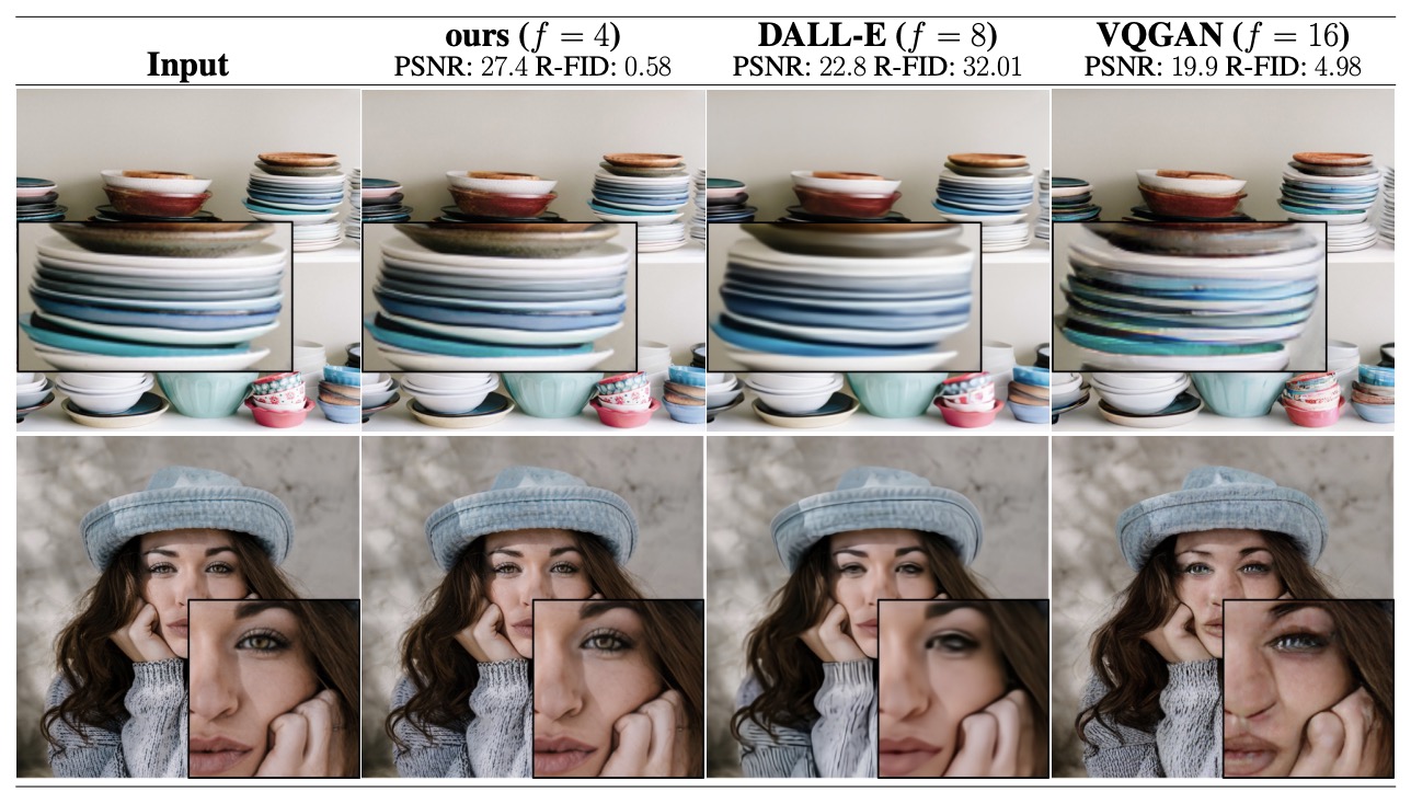
- The following figure (source) illustrates that LDMs are conditioned either via concatenation or by a more general cross-attention mechanism.
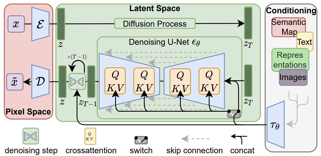
-
The key implementation pattern is two-stage training:
\[z=E(x), \qquad \hat{x}=D(z)\] \[\mathcal{L}_{\text{LDM}}= \mathbb{E}_{E(x),\epsilon,t} \left[ \left| \epsilon-\epsilon_\theta(z_t,t,c) \right|_2^2 \right]\]- where \(E\) and \(D\) are an autoencoder pair, and \(\epsilon_\theta\) is the denoising model trained over latent variables rather than pixels. High-Resolution Image Synthesis with Latent Diffusion Models by Rombach et al. (2022) also introduced cross-attention conditioning for text, semantic maps, and other structured inputs, making latent diffusion a general-purpose renderer architecture.
-
The following figure (source) shows perceptual and semantic compression, where the autoencoder removes imperceptible details before the diffusion model learns the semantic generative distribution. Most bits of a digital image correspond to imperceptible details. While DMs allow to suppress this semantically meaningless information by minimizing the responsible loss term, gradients (during training) and the neural network backbone (training and inference) still need to be evaluated on all pixels, leading to superfluous computations and unnecessarily expensive optimization and inference. We propose latent diffusion models (LDMs) as an effective generative model and a separate mild compression stage that only eliminates imperceptible details.
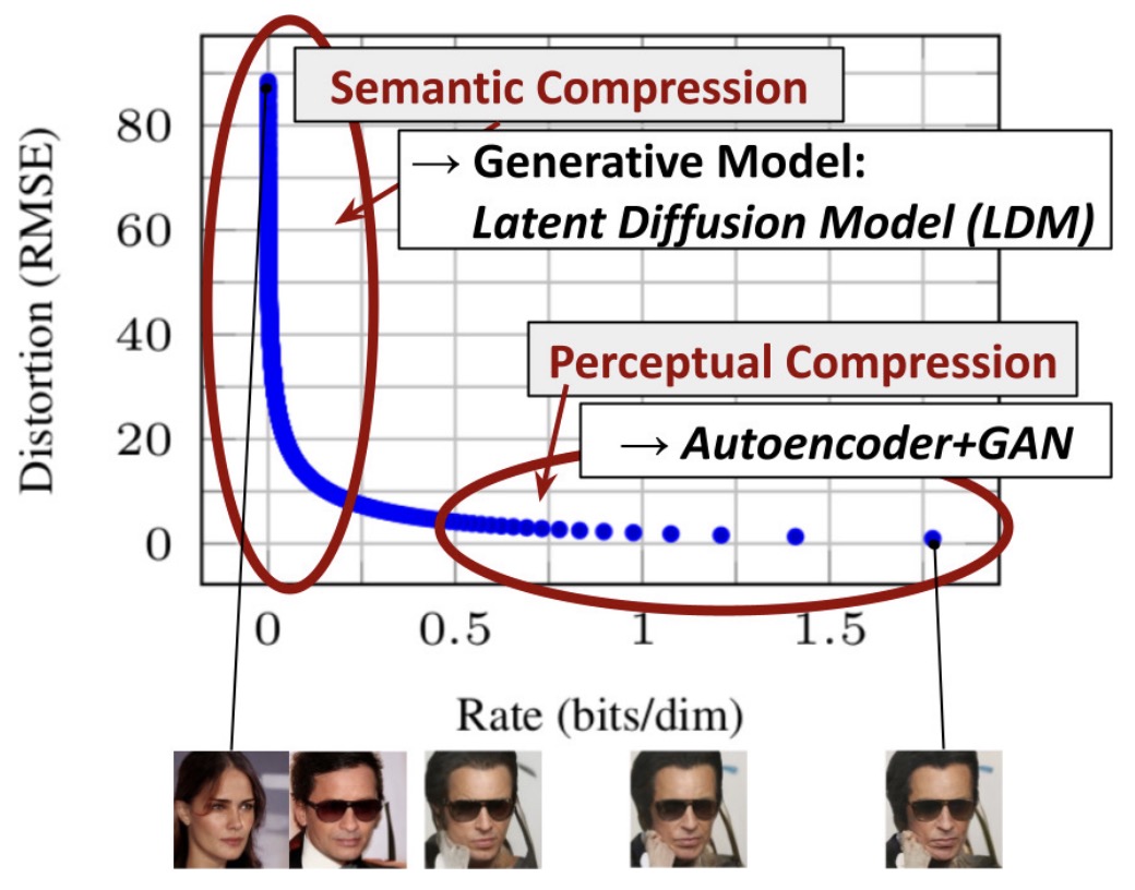
Conditioning and Guidance
-
Renderer world models become useful when they are controllable. Conditioning can enter through concatenation, cross-attention, adaptive normalization, or in-context tokens. For text-to-image and text-to-video systems, cross-attention is especially important because it binds visual tokens to language tokens.
-
Classifier-free guidance is a common sampling-time method for strengthening conditioning:
\[\tilde{\epsilon}_\theta(x_t,c) =\epsilon_\theta(x_t,\varnothing) + s\left(\epsilon_\theta(x_t,c)-\epsilon_\theta(x_t,\varnothing)\right)\]- where \(s\) is the guidance scale. Video Diffusion Models by Ho et al. (2022) uses classifier-free guidance in video generation and extends the image diffusion recipe to temporally coherent frame blocks.
-
Guidance improves adherence but can reduce diversity. This is a core renderer trade-off: stronger conditioning makes generated observations more faithful to a prompt or action, but may narrow the distribution of plausible worlds.
Video Diffusion as Temporal Rendering
- Video renderer models extend image diffusion from a single observation to a block of observations:
-
The simplest version denoises an entire spatiotemporal block. Video Diffusion Models by Ho et al. (2022) extends image U-Nets into factorized space-time 3D U-Nets, adding temporal attention after spatial attention so the model can jointly represent appearance and motion.
-
For long videos, short-horizon generation must be extended. Video Diffusion Models by Ho et al. (2022) introduces reconstruction-guided conditional sampling for temporal extension and spatial super-resolution, showing how fixed-window diffusion models can generate longer and higher-resolution sequences.
-
A renderer video model therefore has two coupled requirements:
- Spatial fidelity: each frame must look plausible and detailed.
- Temporal fidelity: identities, motion, geometry, and scene layout must remain coherent across time.
-
The first requirement is inherited from image generation; the second is what makes video generation world-model-like.
Transformer Backbones for Renderer Scaling
-
As renderer models scale, transformer backbones become increasingly important. Scalable Diffusion Models with Transformers by Peebles and Xie (2023) replaces the U-Net backbone with a Diffusion Transformer (DiT) that operates over latent patches and finds that increasing forward-pass compute through depth, width, or token count consistently improves sample quality.
-
The following figure (source) shows the Diffusion Transformer architecture, where a noised latent is patchified into tokens and processed by transformer blocks with conditioning through adaptive layer normalization, cross-attention, or in-context tokens. Specifically: (Left) They train conditional latent DiT models. The input latent is decomposed into patches and processed by several DiT blocks. Right: Details of our DiT blocks. They experiment with variants of standard transformer blocks that incorporate conditioning via adaptive layer norm, cross-attention and extra input tokens. Adaptive layer norm works best.
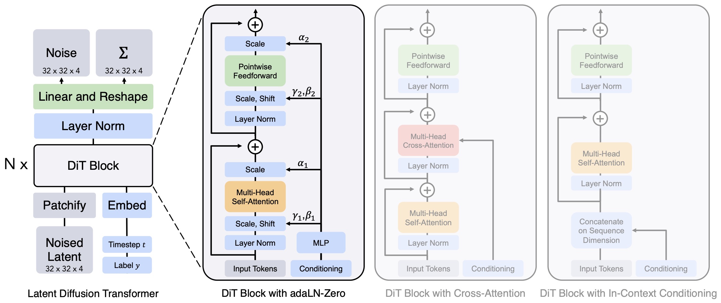
- A DiT-style renderer follows the same latent diffusion objective, but changes the denoiser:
- This architectural shift matters because renderer world models increasingly need the same scaling properties that made transformers successful in language and representation learning.
Renderer World Models versus Latent Simulator Models
- Renderer world models optimize observation likelihood or denoising quality. A renderer objective can be summarized as:
- A latent simulator objective instead predicts compact state:
- The distinction is not absolute. Many modern systems combine both: a latent world model predicts compressed future tokens, and a renderer decodes those tokens into pixels. GAIA-1: A Generative World Model for Autonomous Driving by Hu et al. (2023) explicitly separates an autoregressive token world model from a video diffusion decoder, using the first for high-level dynamics and the second for high-quality rendering.
Practical Implementation Pattern
-
A renderer world model usually contains the following components:
- Tokenizer or autoencoder: compresses observations into latent tokens.
- Generative backbone: U-Net, DiT, spatiotemporal transformer, or autoregressive transformer.
- Conditioning interface: text, image, video prefix, camera path, action sequence, layout, or multimodal tokens.
- Sampler: DDPM, DDIM, predictor-corrector, diffusion forcing, or autoregressive decoding.
- Decoder: maps latent samples back to pixels or video frames.
-
A typical latent diffusion renderer training step is:
x = sample_images_or_video()
z = encoder(x).detach()
t = sample_noise_level()
eps = torch.randn_like(z)

z_t = alpha[t] * z + sigma[t] * eps
eps_pred = denoiser(z_t, t, conditioning)

loss = mse(eps_pred, eps)
loss.backward()
optimizer.step()
- For video, the tensor shape changes from image latents to spatiotemporal latents \(z \in \mathbb{R}^{T \times H \times W \times C}\) and the model must decide whether to use full spatiotemporal attention, factorized space-time attention, frame stacking, temporal cross-attention, or causal autoregressive generation.
Strengths and Limitations
-
Renderer world models are strongest when the goal is visual imagination, content creation, synthetic data generation, or human-interpretable rollouts. They can generate high-fidelity scenes, interpolate missing frames, extend video, and produce visually rich counterfactuals.
-
Their limitations are equally important:
- Visual realism does not guarantee physical correctness.
- Pixel-level objectives can spend capacity on irrelevant details.
- Long-horizon consistency remains difficult.
- Action conditioning can drift if the model treats actions as weak visual prompts rather than causal interventions.
- Generated observations may not expose editable, inspectable state.
-
This is why renderer world models are best treated as one branch of the world-model taxonomy rather than the whole field. They are essential for observation synthesis, but simulator and planner models are still required when the goal is reliable physical prediction or action selection.
Interactive Renderer World Models
-
Interactive renderer world models extend video generation from passive observation synthesis to action-conditioned visual worlds. Instead of generating a fixed clip from text or an image prompt, they repeatedly accept user or agent actions and render the next observation:
\[\hat{o}_{t+1} \sim p_\theta(o_{t+1}\mid o_{\le t}, a_{\le t}, c)\]- where \(c\) may include a text prompt, image prompt, video context, task description, or domain-specific control signal. This makes the renderer appear simulator-like, because it reacts to actions, but its primary output is still observation-level video rather than an inspectable physical state.
Multimodal Driving Renderers
-
GAIA-1: A Generative World Model for Autonomous Driving by Hu et al. (2023) is a multimodal renderer-world-model hybrid for autonomous driving: it maps video, text, and action inputs into discrete tokens, predicts future tokens autoregressively, and decodes them into realistic driving videos with a diffusion decoder.
-
The architecture separates high-level dynamics from pixel rendering:
-
This split is important because driving requires both semantic control, such as traffic-light state or weather, and action control, such as ego speed or curvature. In renderer terms, GAIA-1 produces visually realistic future observations; in simulator terms, it partially models driving dynamics through token prediction.
-
The following figure (source) shows GAIA-1 generating driving videos under video, text, and action conditioning, including text-conditioned scene changes and ego-action-conditioned rollouts.
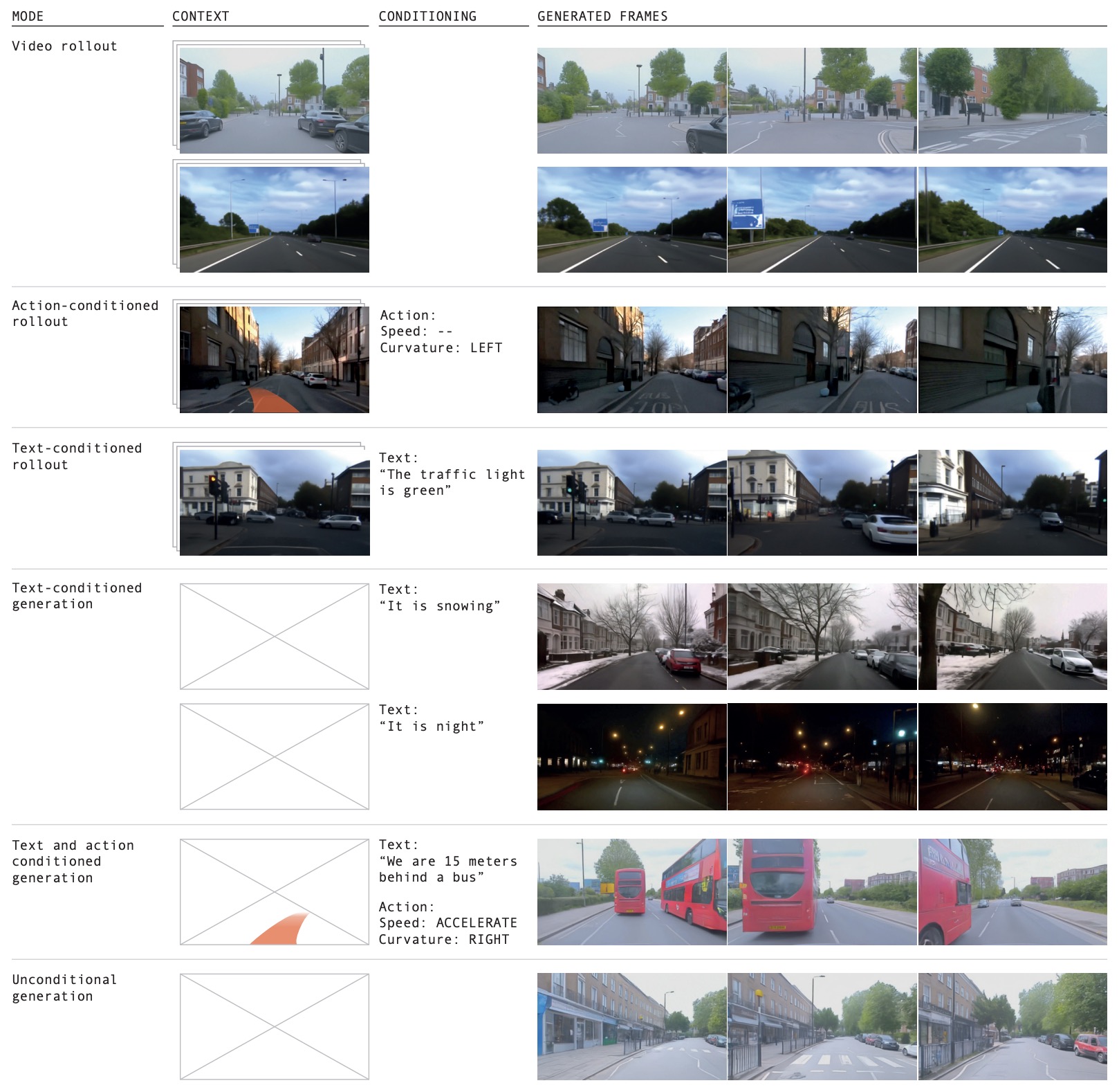
- The following figure (source) shows the GAIA-1 architecture, where video, text, and action encoders produce tokens, an autoregressive transformer predicts future image tokens, and a video decoder renders the output frames.
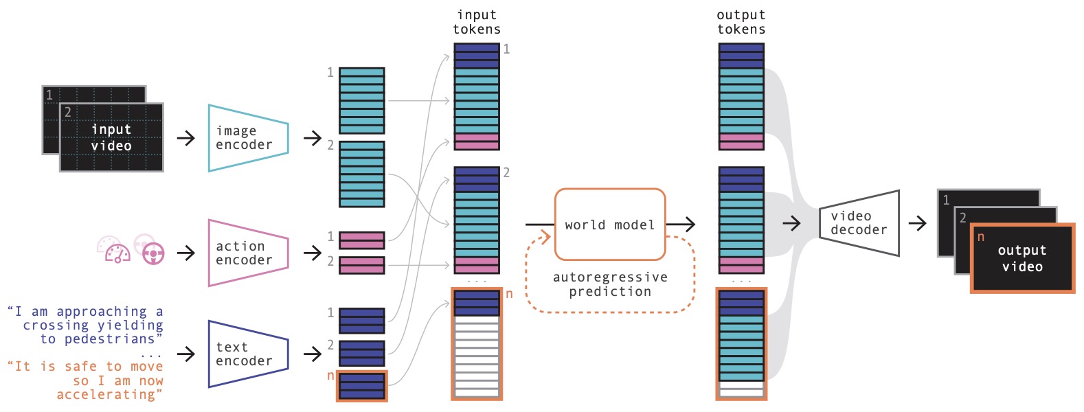
Learned Latent Actions and Playable Worlds
-
Genie: Generative Interactive Environments by Bruce et al. (2024) introduces a foundation world model trained from unlabeled internet videos that can generate playable environments from prompts such as text-to-image outputs, sketches, and photographs.
-
Genie’s distinctive contribution is a learned latent action interface. Because most internet videos lack action labels, Genie infers a discrete latent action space that supports frame-by-frame interaction:
\[\hat{o}_{t+1} \sim p_\theta(o_{t+1}\mid o_{\le t}, \hat{a}_t)\]- where \(\hat{a}_t\) is a learned latent action rather than a human-provided ground-truth control label. This makes it an important renderer-world-model design pattern: actions can be induced from video when explicit control annotations are unavailable.
-
The following figure (source) shows Genie converting text-to-image outputs, hand-drawn sketches, and real-world photos into interactive playable environments through a learned latent action interface.
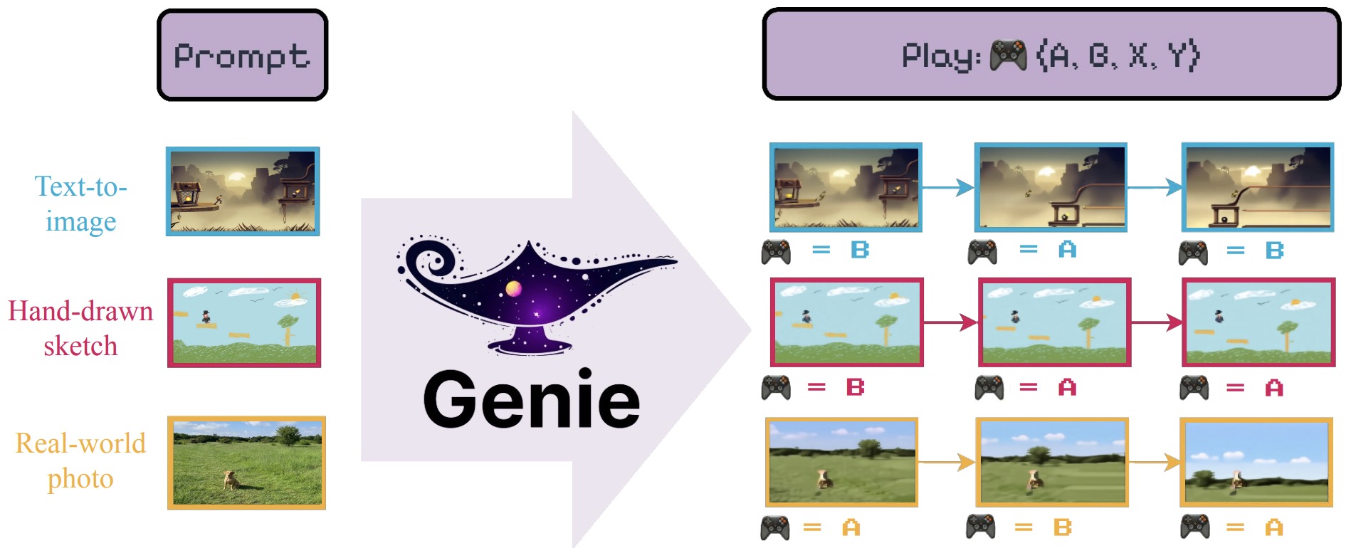
Diffusion Renderers as Game Engines
-
Interactive game renderers make the renderer-simulator boundary especially sharp. A conventional game engine updates hidden state and renders pixels. A neural game renderer instead learns to generate the next frame directly from previous frames and actions.
-
Diffusion Models Are Real-Time Game Engines by Valevski et al. (2024) presents GameNGen, a neural game engine that simulates DOOM in real time by training a diffusion model to generate the next frame conditioned on previous frames and actions.
-
The learned transition is observation-level \(\hat{o}_{t+1}=D_\theta(o_{t-k:t},a_{t-k:t})\) rather than state-level \(\hat{s}_{t+1}=F_\theta(s_t,a_t)\).
-
This is why GameNGen is best categorized as an interactive renderer world model. It can appear to simulate rules, enemies, doors, health, and ammunition, but those variables are not necessarily exposed as editable symbolic state.
-
The following figure (source) shows GameNGen running DOOM at 20 FPS as an interactive neural game engine generated by a diffusion model conditioned on past frames and actions.
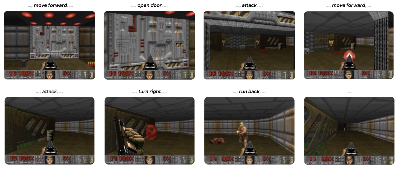
- The following figure (source) overviews the architecture of the GameNGen method.
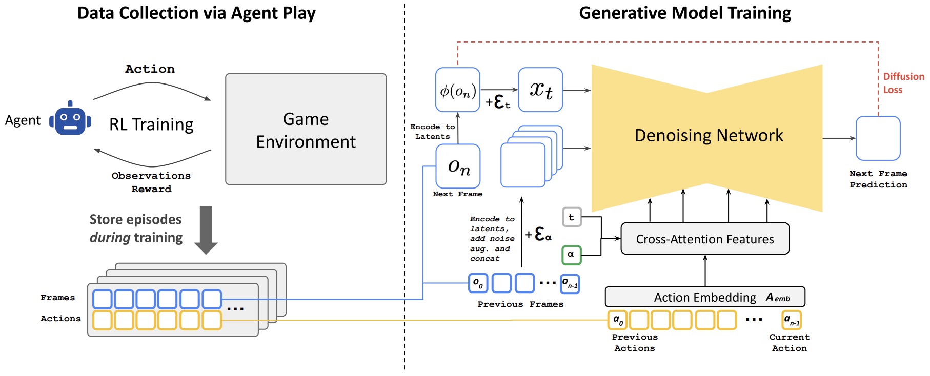
Diffusion World Models for Agent Training
-
Diffusion for World Modeling: Visual Details Matter in Atari by Alonso et al. (2024) introduces DIAMOND, a reinforcement-learning agent trained entirely inside a diffusion world model, arguing that preserving visual details can improve downstream control when small visual cues are task-relevant.
-
DIAMOND unrolls environment imagination autoregressively while running a denoising process at each step \(x_t^T \rightarrow x_t^{T-1} \rightarrow \dots \rightarrow x_t^0\) and then feeds the clean predicted observation into the next imagined transition. This makes it a renderer-planner bridge: the world model renders imagined observations, and the agent learns behavior inside those rendered trajectories.
-
The following figure (source) shows DIAMOND unrolling imagination over environment time while running denoising time vertically for each generated observation.
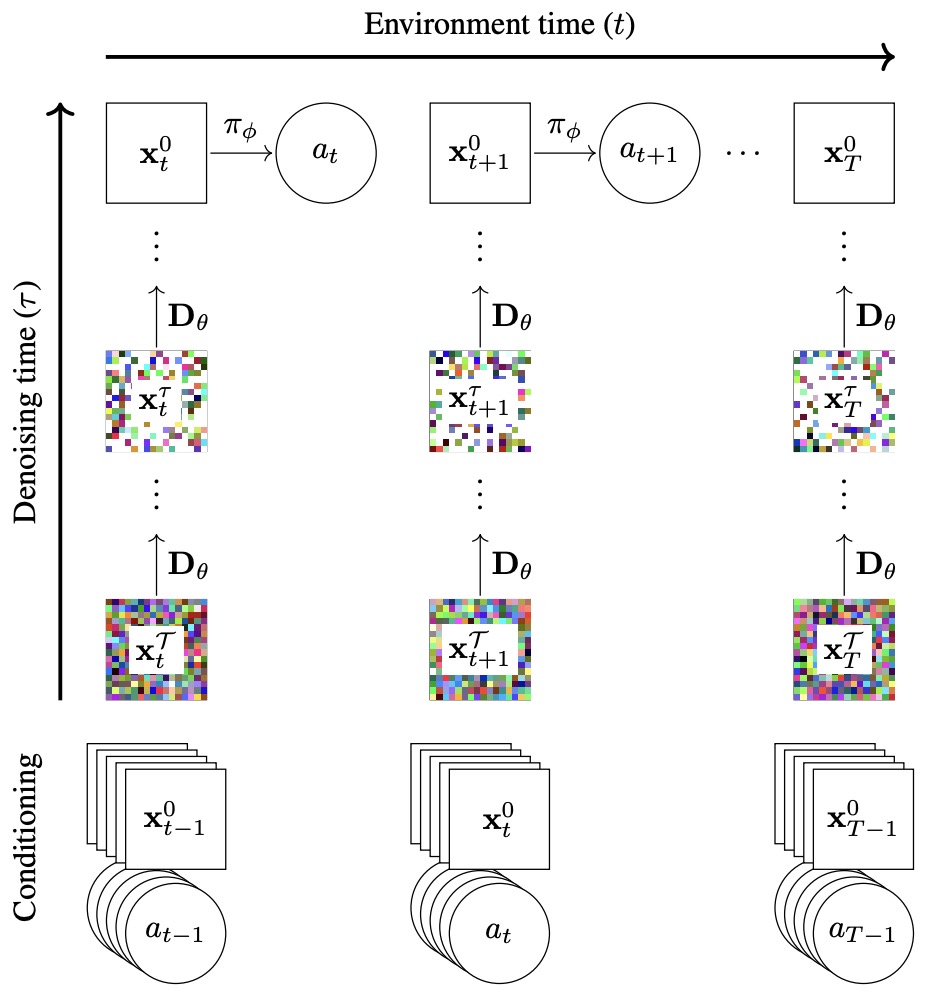
Real-Time Open-World Rendering
-
Oasis: A Universe in a Transformer presents a real-time interactive open-world renderer that takes keyboard input and generates a Minecraft-like experience with graphics, rules, and physics emerging from the model rather than a conventional physics engine.
-
Oasis is important because it highlights the latency constraint for renderer world models. A passive video generator can take seconds or minutes per clip; an interactive renderer must generate frames quickly enough to preserve the action-perception loop:
- The following figure (source) shows the architecture of Oasis, an experiential real-time open-world AI model that generates an interactive Minecraft-like video stream.
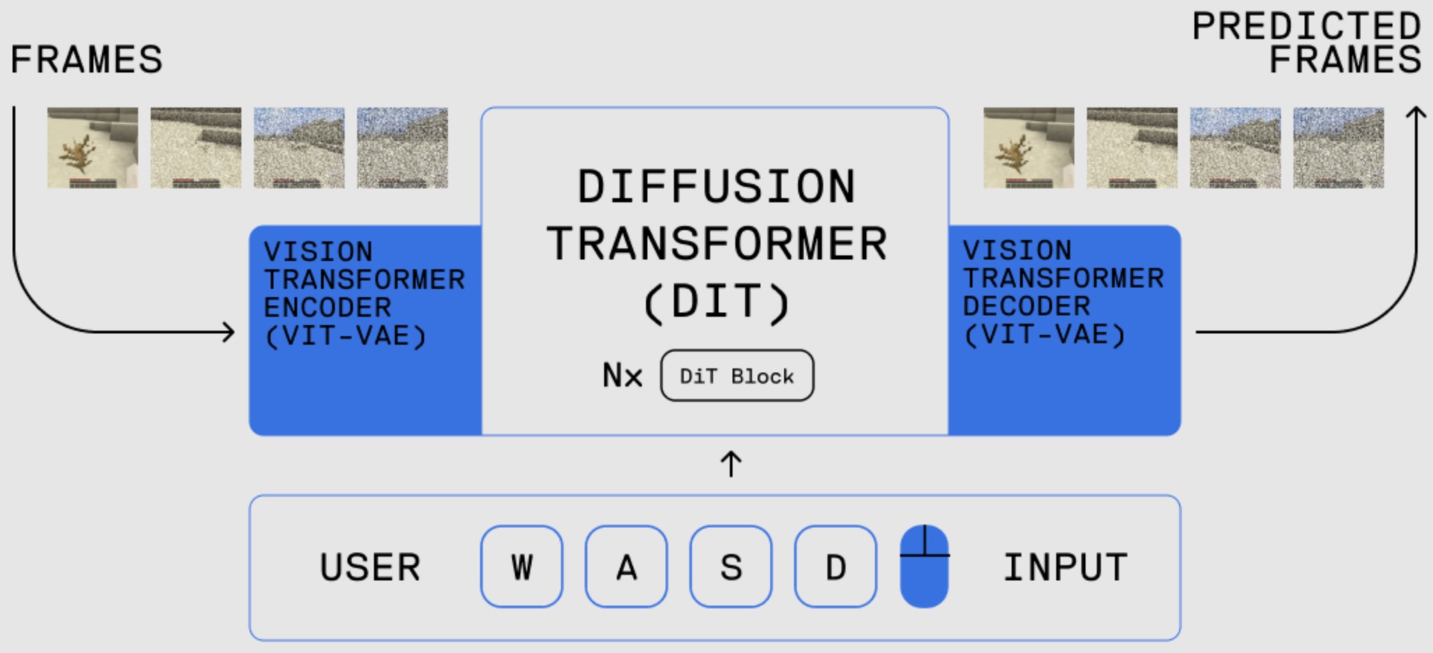
Commercial Text-to-Video Renderers
-
Large text-to-video systems are renderer world models when they generate temporally coherent observations conditioned on prompts. Runway Gen-3 Alpha: Next-Generation AI Video Generation describes a video foundation model trained for fidelity, consistency, and motion, with control modes for text-to-video, image-to-video, camera control, and temporal keyframing.
-
Mochi 1: A new SOTA in open text-to-video describes an open text-to-video model focused on high-fidelity motion and strong prompt adherence.
-
The following figures (source) shows the prompt adherence and motion quality results for Mochi 1 as an open text-to-video system.
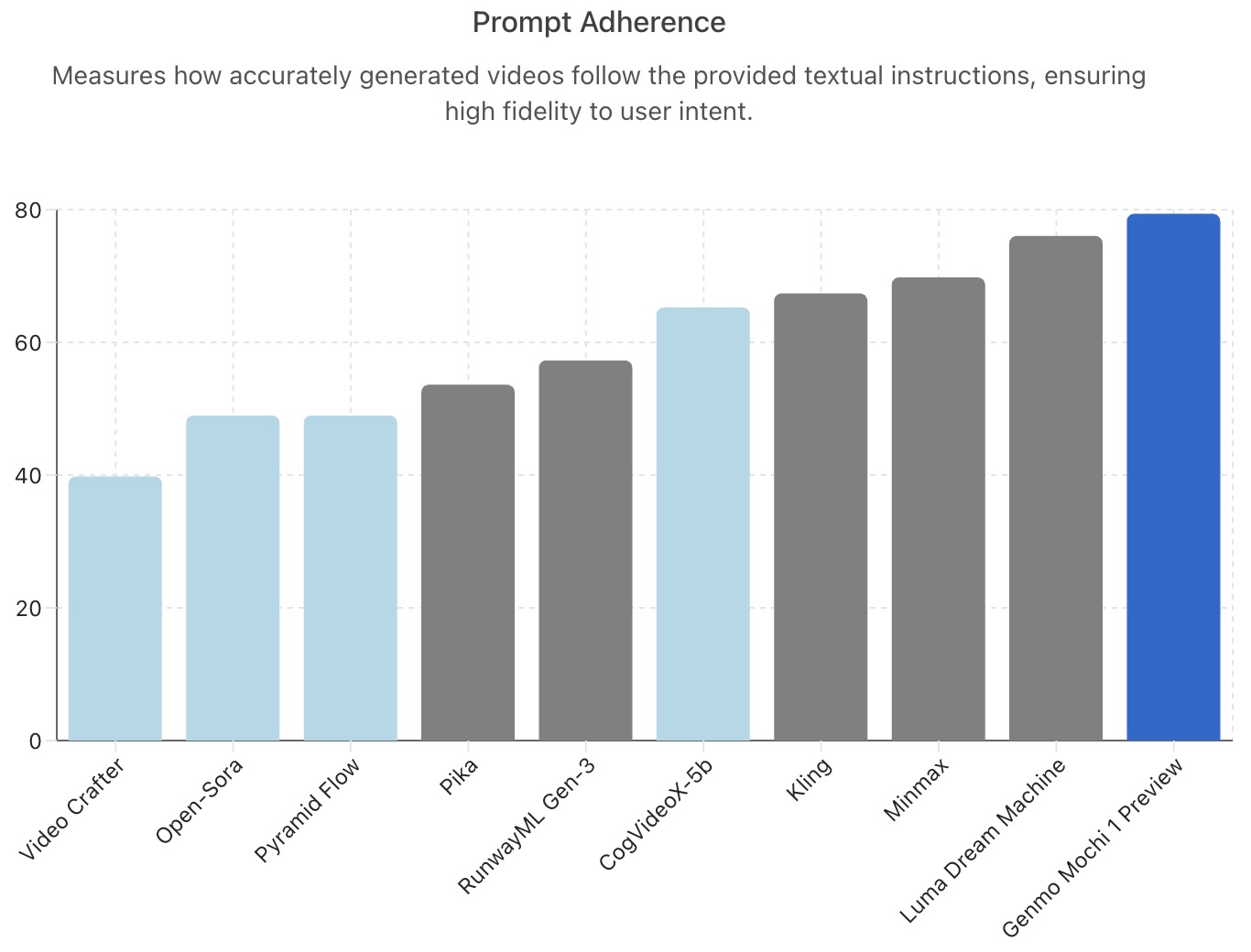
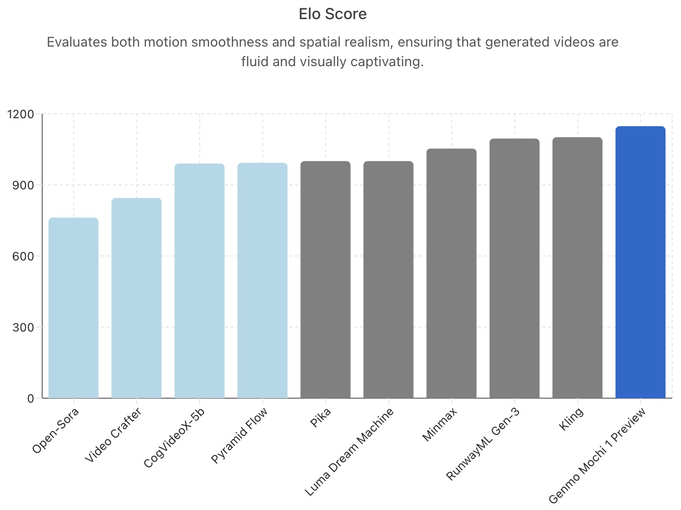
Implementation Pattern for Interactive Renderers
-
Interactive renderer models usually add three components to a standard video generator:
- Action encoder: maps keyboard inputs, robot actions, driving controls, or latent actions into tokens.
- History window: conditions generation on recent frames to preserve temporal continuity.
- Autoregressive rollout mechanism: feeds generated frames back as context for subsequent frames.
-
A generic training objective is:
-
For token-based systems, the objective may instead be autoregressive next-token prediction:
\[\mathcal{L}_{\text{AR}}= -\sum_t \log p_\theta(u_t\mid u_{<t},a_{\le t},c)\]- where \(u_t\) is a visual token. GAIA-1 uses this token-prediction pattern before decoding predicted tokens with a diffusion video decoder. GAIA-1 by Hu et al. (2023) is therefore a hybrid of autoregressive world modeling and diffusion rendering.
Failure Modes and Evaluation
-
Interactive renderer world models should be evaluated on more than visual quality. Key metrics include:
- Action adherence: whether the rendered future reflects the control input.
- Temporal stability: whether identities, layout, and object states persist over long rollouts.
- Rule consistency: whether game or driving rules remain stable.
- Recoverability: whether errors compound or self-correct.
- Latency: whether generation is fast enough for closed-loop interaction.
- Visual detail preservation: whether small task-relevant details survive compression.
-
This last point is important in control domains. Diffusion for World Modeling: Visual Details Matter in Atari by Alonso et al. (2024) argues that visual details lost by compact discrete latents can matter for reinforcement learning, motivating diffusion renderers as trainable environments.
Relationship to JEPA
- Interactive renderer world models and JEPA world models optimize different contracts. A renderer predicts observations:
- A JEPA predicts latent state:
- The renderer is easier to inspect because it outputs pixels. JEPA is often more efficient for planning because it avoids rendering irrelevant detail. A mature world-model stack may combine both: a JEPA-style latent simulator for compact planning and a renderer module for visualization, data generation, or human-facing interaction.
Design Trade-offs and Evaluation
Observation Fidelity versus State Fidelity
- Renderer world models optimize the quality of generated observations. Their natural objective is to produce frames or videos that are visually plausible, temporally coherent, and aligned with conditioning:
-
This makes them powerful for imagination, content creation, synthetic data generation, and interactive visual environments. Video Diffusion Models by Ho et al. (2022) shows that diffusion models can generate coherent video by extending image diffusion architectures to spatiotemporal data, while GAIA-1: A Generative World Model for Autonomous Driving by Hu et al. (2023) shows that video, text, and action conditioning can be combined to render controllable driving futures.
-
The central limitation is that observation fidelity does not imply state fidelity. A renderer can generate a realistic-looking scene while failing to maintain the exact hidden state required for physics, robotics, or safety-critical planning. In a simulator-first model, the primary object is instead a state transition:
- The distinction matters because an action-conditioned renderer may appear to simulate the world, but its internal state may remain implicit, distributed, and difficult to inspect. Diffusion Models Are Real-Time Game Engines by Valevski et al. (2024) demonstrates that a diffusion model can render an interactive DOOM-like game stream in real time, but the learned engine is still observation-output-first rather than an explicit symbolic or physical simulator.
Long-Horizon Consistency
- Long-horizon consistency is the main technical challenge for renderer world models. In autoregressive video rendering, each generated frame becomes part of the conditioning context for later frames:
-
Small visual or semantic errors can compound over time, causing identity drift, geometry drift, texture instability, or inconsistent object state. Diffusion Forcing: Next-token Prediction Meets Full-Sequence Diffusion by Chen et al. (2024) addresses this by assigning independent noise levels to sequence tokens, combining the variable-horizon flexibility of next-token prediction with the trajectory guidance benefits of full-sequence diffusion.
-
For interactive settings, long-horizon consistency is not merely an aesthetic property. It determines whether the model can preserve an agent’s location, inventory, road context, collision history, or object permanence across repeated user interventions. Genie: Generative Interactive Environments by Bruce et al. (2024) is important here because it learns a latent action interface from unlabeled internet video, allowing generated environments to be stepped through frame by frame.
Action Adherence and Controllability
- Renderer world models become world-model-like when they respond reliably to actions. A text-to-video model can render plausible motion, but an interactive renderer must bind controls to consequences:
-
This requires the model to distinguish between visual correlation and causal control. GAIA-1 by Hu et al. (2023) conditions driving rollouts on ego-vehicle speed and curvature, making control adherence a core part of the generated future. Oasis: A Universe in a Transformer presents an interactive open-world model where keyboard inputs are mapped directly into a generated Minecraft-like visual stream.
-
A practical renderer evaluation should therefore measure whether the action affects the correct visual variables. Steering should change ego trajectory, jumping should change camera height and scene dynamics, breaking an object should persist in later frames, and a traffic-light edit should remain stable across the rollout.
Visual Detail as a Control Signal
-
One reason renderer world models remain relevant for control is that visual details can matter. Compact latent models may discard small cues that are irrelevant for reconstruction metrics but crucial for reward or safety. Diffusion for World Modeling: Visual Details Matter in Atari by Alonso et al. (2024) argues that diffusion world models can improve agent training when task-relevant details would otherwise be lost through overly compressed discrete latents.
-
This point creates a nuanced trade-off. JEPA-style latent simulators avoid wasting capacity on unpredictable detail, but renderer models may preserve low-level signals that matter for certain tasks. A pedestrian far away, a small traffic light, a projectile, a door handle, or an inventory icon may be visually small but decision-critical.
Evaluation Criteria for Renderer World Models
-
Renderer world models should be evaluated by a packed set of criteria: visual fidelity should measure frame-level realism and perceptual quality; temporal coherence should measure identity, layout, and object-state persistence; controllability should measure whether text, camera, action, or layout conditions reliably affect the intended variables; long-horizon stability should measure compounding error across autoregressive rollouts; physical plausibility should measure whether motion, contact, and geometry remain believable; and task utility should measure whether generated observations help downstream agents, planners, or users.
-
This broader evaluation lens is necessary because classic image and video metrics alone are insufficient. A model can score well on perceptual realism yet fail as a world model if it ignores actions, violates persistence, or produces futures that are visually plausible but causally wrong.
Relationship to JEPA
- Renderer world models and JEPA-style world models occupy complementary positions. Renderer models optimize observation generation:
- JEPA-style models optimize latent prediction:
- The renderer objective is useful when the system must show or synthesize the world. The JEPA objective is useful when the system must reason over compact predictable structure. A mature world-model stack may use both: a renderer for visualization and synthetic experience, a simulator-style latent model for efficient prediction, and a planner for goal-directed action selection.
Simulator World Models
Neural Scene and Spatial State Representations
-
Simulator world models are systems whose primary output is state rather than raw observation. A renderer asks what the world should look like; a simulator asks what the world is and how that state can be queried, transformed, rendered, or rolled forward. In spatial domains, this state may be a continuous radiance field, a Gaussian-splat scene, a mesh, a point cloud, a signed-distance field, an object layout, or a hybrid neural representation.
-
A spatial simulator can be written as:
\[z = \mathcal{S}_\theta(o_{1:N}, c_{1:N})\]- where \(o_{1:N}\) are observations and \(c_{1:N}\) are camera poses, calibration parameters, or conditioning inputs. Once learned, the simulator exposes a state representation \(z\) that can be rendered from new viewpoints, edited, optimized, or combined with downstream planning systems.
Neural Radiance Fields as Continuous Scene Simulators
-
NeRF: Representing Scenes as Neural Radiance Fields for View Synthesis by Mildenhall et al. (2020) represents a scene as a continuous function that maps 3D position and viewing direction to density and color, making it a foundational neural scene simulator for novel-view synthesis.
\[F_\theta:(x,y,z,\theta,\phi)\rightarrow(\sigma,c)\]- where \(\sigma\) is volume density and \(c\) is view-dependent emitted radiance. Rendering is performed by sampling points along camera rays and integrating color through differentiable volume rendering:
-
This makes NeRF simulator-like because it does not merely generate a single image. It learns a continuous 3D scene function that can be queried from novel camera viewpoints. The implementation depends on camera-calibrated image collections, positional encoding for high-frequency details, hierarchical ray sampling, and optimization through photometric reconstruction loss. NeRF by Mildenhall et al. (2020) introduced positional encoding and differentiable volume rendering as practical tools for optimizing photorealistic neural scene representations from posed RGB images.
-
The following figure (source) shows the NeRF pipeline, where camera rays are sampled through a continuous 5D radiance field and accumulated with differentiable volume rendering to synthesize novel views. They use techniques from volume rendering to accumulate samples of this scene representation along rays to render the scene from any viewpoint. Here, we visualize the set of 100 input views of the synthetic Drums scene randomly captured on a surrounding hemisphere, and we show two novel views rendered from our optimized NeRF representation.
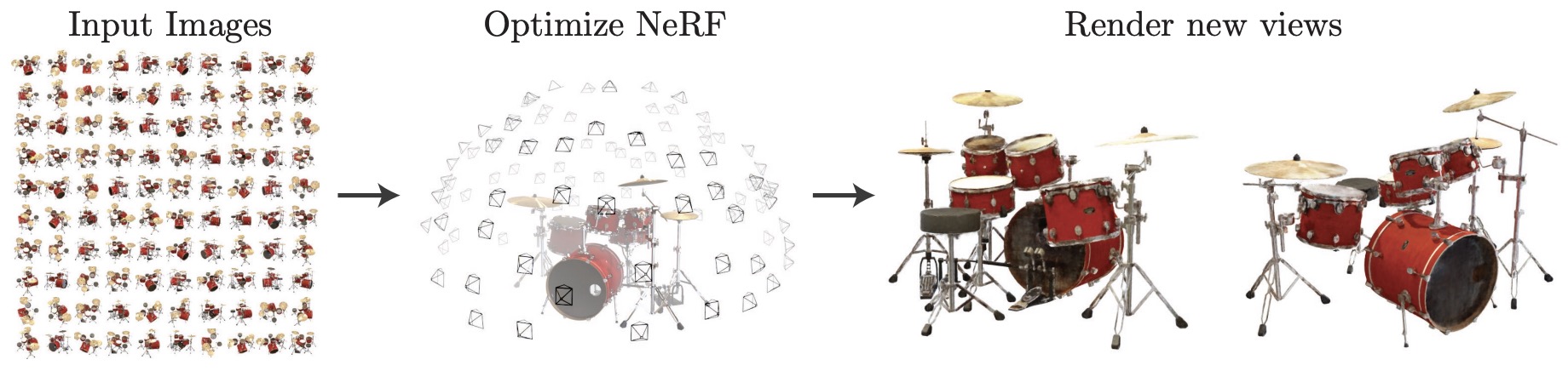
- The following figure (source) shows an overview of the NeRF scene representation and differentiable rendering procedure. We synthesize images by sampling 5D coordinates (location and viewing direction) along camera rays (a), feeding those locations into an MLP to produce a color and volume density (b), and using volume rendering techniques to composite these values into an image (c). This rendering function is differentiable, so we can optimize our scene representation by minimizing the residual between synthesized and ground truth observed images (d).
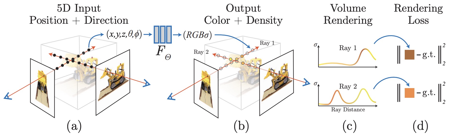
Explicit Neural Scene State through 3D Gaussian Splatting
-
3D Gaussian Splatting for Real-Time Radiance Field Rendering by Kerbl et al. (2023) moves neural scene simulation toward an explicit point-based representation by modeling scenes as anisotropic 3D Gaussians optimized from structure-from-motion points.
-
Each Gaussian has position, opacity, covariance, and view-dependent color parameters:
-
Rendering projects Gaussians into screen space and alpha-composites them in visibility order:
\[C=\sum_i T_i \alpha_i c_i\]- where \(T_i\) is accumulated transmittance from earlier splats. This representation is simulator-like because the scene is no longer hidden entirely inside an MLP; it is stored as an editable set of spatial primitives that can be rendered in real time. 3D Gaussian Splatting for Real-Time Radiance Field Rendering by Kerbl et al. (2023) reports real-time rendering at 1080p using anisotropic 3D Gaussians, adaptive density control, and a visibility-aware tile rasterizer.
-
The following figure (source) shows 3D Gaussian Splatting achieving real-time rendering quality competitive with prior radiance-field methods while reducing optimization and rendering cost.
- The following figure (source) shows the 3D Gaussian Splatting optimization pipeline, where sparse SfM points initialize Gaussians, adaptive density control refines the representation, and a differentiable tile rasterizer provides gradients for optimization.

- An implementation typically starts from calibrated images and a sparse structure-from-motion point cloud, initializes Gaussians at point locations, optimizes opacity and spherical-harmonic color coefficients, adapts Gaussian density by splitting or pruning primitives, and minimizes a photometric loss such as:
- The engineering significance is that 3D Gaussian Splatting narrows the gap between neural world representations and interactive simulators: the learned state is explicit enough for fast rendering, yet continuous enough to retain radiance-field quality.
Text-to-3D as Generative Spatial Simulation
-
DreamFusion: Text-to-3D using 2D Diffusion by Poole et al. (2022) uses a pretrained 2D text-to-image diffusion model as a prior for optimizing a 3D representation, showing that a renderer-style generative model can supervise a simulator-style 3D state without requiring large-scale labeled 3D data.
-
DreamFusion optimizes a randomly initialized NeRF so that random renderings of the 3D object are scored as likely by a text-conditioned diffusion model. Its core training mechanism is score distillation sampling:
\[\nabla_\theta \mathcal{L}_{\text{SDS}}(\theta) =\mathbb{E}_{t,\epsilon} \left[ w(t) \left( \epsilon_\phi(x_t;y,t)-\epsilon \right) \frac{\partial x}{\partial \theta} \right]\]- where \(\epsilon_\phi\) is the pretrained diffusion denoiser, \(y\) is the text prompt, and \(x\) is a rendered image of the current 3D representation. DreamFusion by Poole et al. (2022) is important for simulator world models because it converts a 2D generative prior into an optimizable 3D scene state that can be viewed from arbitrary angles.
-
The following figure (source) shows the DreamFusion optimization loop, where a text-conditioned diffusion prior supplies gradients to a rendered view of a 3D model, gradually shaping a coherent text-conditioned 3D representation. DreamFusion generates 3D objects from a natural language caption such as “a DSLR photo of a peacock on a surfboard.” The scene is represented by a Neural Radiance Field that is randomly initialized and trained from scratch for each caption. Our NeRF parameterizes volumetric density and albedo (color) with an MLP. We render the NeRF from a random camera, using normals computed from gradients of the density to shade the scene with a random lighting direction. Shading reveals geometric details that are ambiguous from a single viewpoint. To compute parameter updates, DreamFusion diffuses the rendering and reconstructs it with a (frozen) conditional Imagen model to predict the injected noise \(\hat{\epsilon}_\phi\left(\mathbf{z}_t \mid y ; t\right)\). This contains structure that should improve fidelity, but is high variance. Subtracting the injected noise produces a low variance update direction stopgrad \(\left[\hat{\epsilon}_\phi-\epsilon\right]\) that is backpropagated through the rendering process to update the NeRF MLP parameters.
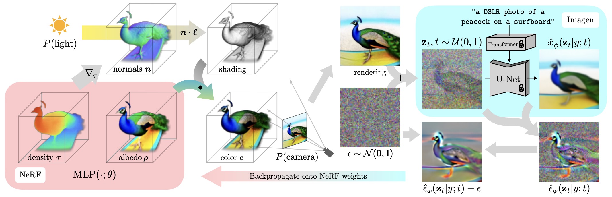
- This is a bridge between renderer and simulator paradigms. The supervising model is a renderer because it evaluates images, but the optimized object is a simulator-compatible 3D state. This pattern has become central to text-to-3D, embodied simulation, game asset generation, and spatial AI pipelines.
Visual De-animation and Inverse Graphics as Simulator Construction
-
Learning to See Physics via Visual De-animation by Wu et al. (2017) frames scene understanding as recovering a physical world representation from visual input, then using physics and graphics engines to reason forward and render predicted outcomes.
-
The model decomposes visual understanding into inverse graphics, physical-state estimation, forward simulation, and rendering:
-
This is simulator-first because the core latent object is physical state: positions, velocities, masses, friction, shape, viewpoint, and scene layout. The perception module infers this state, the physics engine rolls it forward, and the graphics engine renders outcomes for reconstruction or prediction. Learning to See Physics via Visual De-animation by Wu et al. (2017) shows how inverse graphics and physics simulation can be combined so that visual prediction is mediated by an interpretable physical representation.
-
The following figure (source) shows visual de-animation, where the system recovers the physical world representation behind visual input and combines it with physics simulation and rendering engines.
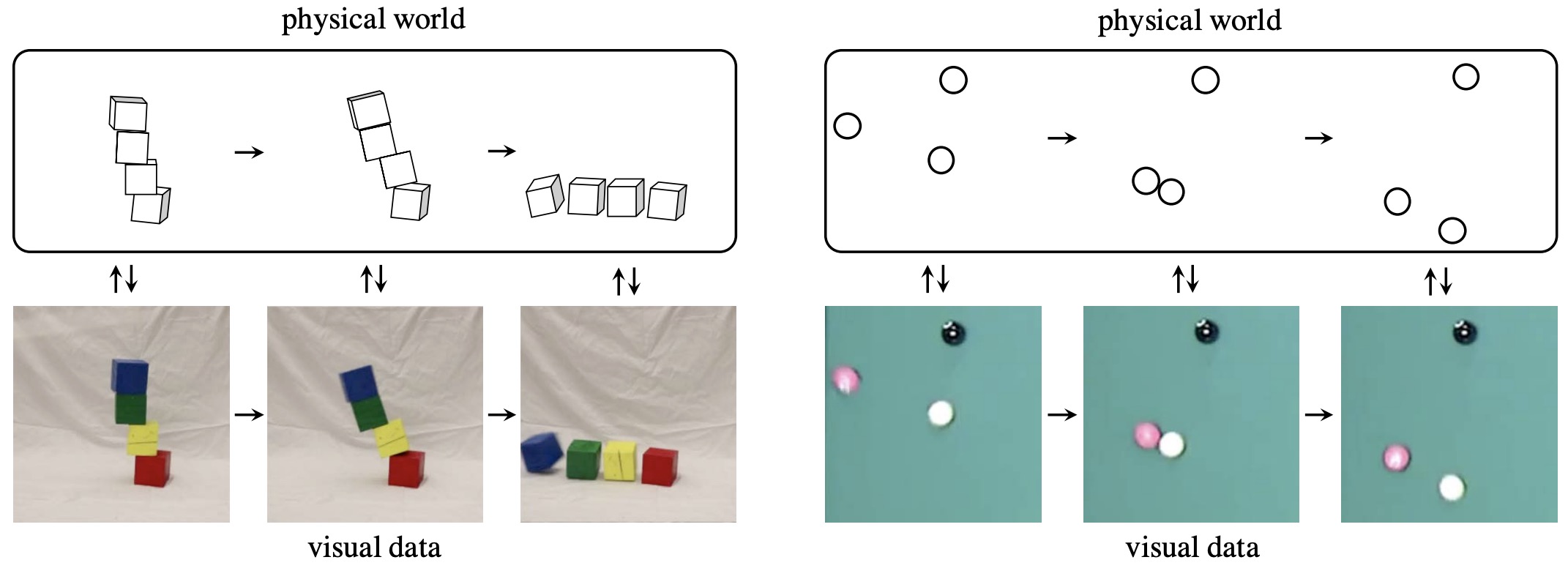
- The following figure (source) shows the visual de-animation framework, including inverse graphics, physical state recovery, physics-based future prediction, and rendering-based reconstruction. Specifically, visual de-animation (VDA) model contains three major components: a convolutional perception module (I), a physics engine (II), and a graphics engine (III). The perception module efficiently inverts the graphics engine by inferring the physical object state for each segment proposal in input (a), and combines them to obtain a physical world representation (b). The generative phyand graphics engines then run forward to reconstruct the visual data (e).
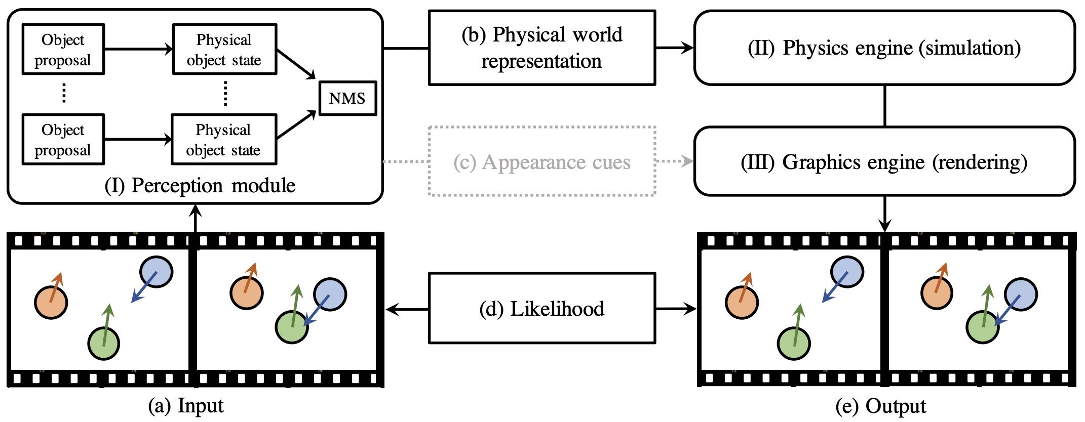
- A practical version of this pipeline uses an object detector or proposal generator, a neural network for object and physical-parameter inference, a differentiable or non-differentiable physics engine, and a rendering loss that forces the inferred state to explain observations. In differentiable settings, gradients can flow from image reconstruction through rendering into physical-state estimates. In non-differentiable settings, state inference may rely on learned approximations, search, or surrogate gradients.
Implementation Pattern for Spatial Simulator World Models
-
A spatial simulator world model generally follows a packed implementation pattern: it first defines a state representation such as a radiance field, Gaussian splat field, mesh, point cloud, or object-physical state; it then defines a differentiable or approximately differentiable renderer that maps state to observations; it optimizes the state or neural parameters against observed images, videos, poses, or text-conditioned priors; and it exposes the learned state for novel-view rendering, editing, simulation, or downstream planning.
-
The generic objective is:
\[\mathcal{L}_{\text{sim-state}} =\mathcal{L}_{\text{render}}(R_\psi(z),o) +\lambda\mathcal{L}_{\text{state-prior}}(z) +\gamma\mathcal{L}_{\text{consistency}}(z)\]- where \(R_\psi\) is a renderer, \(z\) is the learned scene state, and the regularization terms encode priors such as smoothness, sparsity, geometric consistency, multi-view consistency, or physical plausibility.
Learned Physical Dynamics and Relational Simulation
From Static Scene State to Dynamic State Transition
-
A spatial scene representation becomes a simulator when it can predict how the state evolves under time, forces, contacts, constraints, or actions. The core simulator equation is:
\[\hat{z}_{t+1}=F_\theta(z_t,a_t)\]- where \(z_t\) is the current world state and \(a_t\) may represent an external action, control input, force, boundary condition, or intervention. In a physical simulator, the state must preserve quantities that support prediction, such as position, velocity, mass, material properties, object identity, contact state, and relation structure.
-
Learned physical simulators differ from renderer world models because they do not primarily optimize for image realism. Their target is state fidelity: the predicted future state should obey the learned dynamics of interacting entities, fluids, cloth, rigid bodies, deformable materials, or meshes.
Interaction Networks and Object-Relation Simulation
-
Interaction Networks for Learning about Objects, Relations and Physics by Battaglia et al. (2016) introduced a neural framework for reasoning over objects and relations, where the model takes object states and relation attributes as input, computes interaction effects, and applies learned object dynamics to predict future states. ([NeurIPS Proceedings][1])
-
The state is naturally graph-structured:
\[G_t=(V_t,E_t)\]- where each node \(v_i \in V_t\) represents an object and each edge \(e_{ij}\in E_t\) represents a relation or interaction. The model computes relation effects and aggregates them into object updates:
-
This architecture is simulator-like because it mirrors the compositional structure of physical systems: objects interact through relations, and future state emerges from those interactions. Interaction Networks by Battaglia et al. (2016) showed that object-relation neural computation can simulate n-body systems, rigid-body collisions, and non-rigid dynamics while generalizing across different object configurations.
-
The following figure (source) shows an interaction network, where objects and relations are encoded, interaction effects are computed, and object dynamics are applied to produce physical predictions. Specifically: a. For physical reasoning, the model takes objects and relations as input, reasons about their interactions, and applies the effects and physical dynamics to predict new states. b. For more complex systems, the model takes as input a graph that represents a system of objects, \(o_j\), and relations, \(\left\langle i, j, r_k\right\rangle_k\), instantiates the pairwise interaction terms, \(b_k\), and computes their effects, \(e_k\), via a relational model, \(f_R(\cdot)\). The \(e_k\) are then aggregated and combined with the \(o_j\) and external effects, \(x_j\), to generate input (as \(c_j\)), for an object model, \(f_O(\cdot)\), which predicts how the interactions and dynamics influence the objects, \(p\).
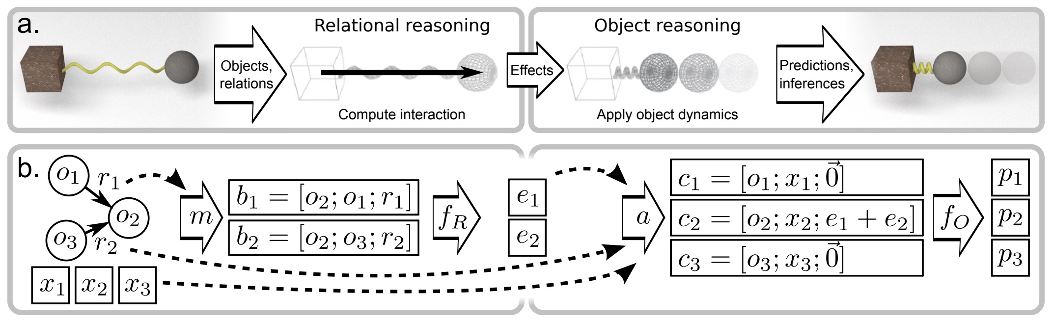
Visual Interaction Networks and Simulation from Video
-
Visual Interaction Networks: Learning a Physics Simulator from Video by Watters et al. (2017) extends object-relation simulation to raw visual input by using a perceptual front-end to infer latent object states and an interaction network to roll those states forward.
-
The model can be summarized as:
\[o_{1:k}\rightarrow {z_k^{(1)},z_k^{(2)},\dots,z_k^{(N)}}\rightarrow \hat{z}_{k+1:k+H}\]- where the first stage parses visual evidence into object-centric latent states and the second stage performs relational dynamics prediction. Visual Interaction Networks by Watters et al. (2017) is important because it connects perception to learned simulation: the model predicts physical trajectories from video rather than requiring direct access to simulator state.
-
The following figure (source) shows the Visual Interaction Network architecture, where a convolutional perceptual front-end infers object states from video and an interaction network predicts future physical trajectories.
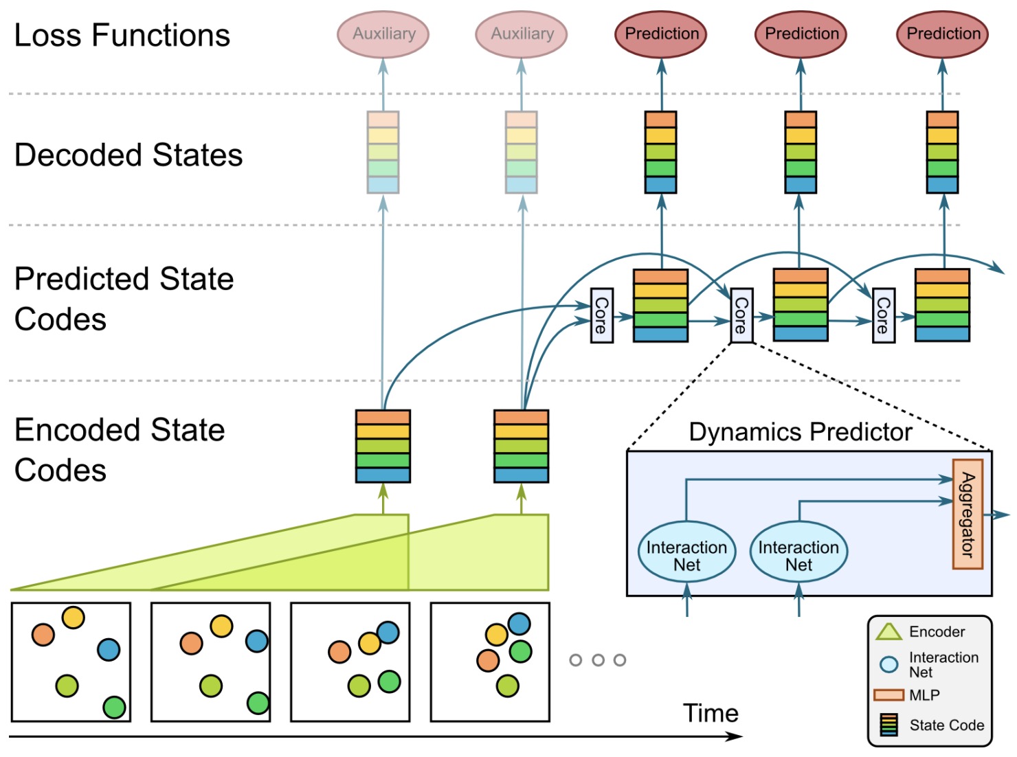
- This pattern remains central to simulator world models. A perception module constructs latent state, a relational dynamics module rolls state forward, and a decoder or evaluator compares predictions to future observations or ground-truth state. Unlike pure video renderers, the goal is not only to synthesize plausible frames; it is to preserve the latent variables that govern future physical behavior.
Graph Network-Based Simulators
-
Learning to Simulate Complex Physics with Graph Networks by Sanchez-Gonzalez et al. (2020) generalizes learned simulation to particle-based physical systems by representing particles as graph nodes and computing dynamics through message passing. ([Proceedings of Machine Learning Research][3])
-
A Graph Network-based Simulator represents each particle or material element as a node:
- Edges connect nearby particles or interacting elements:
- Message passing then computes local interaction effects, aggregates them, and predicts accelerations or position updates:
- The simulator is rolled out autoregressively:
-
Learning to Simulate Complex Physics with Graph Networks by Sanchez-Gonzalez et al. (2020) demonstrated learned simulation across fluids, rigid solids, and deformable materials, and found that noise corruption during training improves robustness to rollout error.
-
The following figure (source) shows the Graph Network-based Simulator framework, where particle states are represented as graph nodes and learned message passing predicts physical evolution. Specifically: (a) The GNS predicts future states represented as particles using its learned dynamics model, \(d_\theta\), and a fixed update procedure. (b) The \(d_\theta\) uses an “encode-process-decode” scheme, which computes dynamics information, \(Y\), from input state, \(X\). (c) The encoder constructs latent graph, \(G^0\), from the input state, \(X\). (d) The processor performs \(M\) rounds of learned message-passing over the latent graphs, \(G^0, \ldots, G^M\). (e) The decoder extracts dynamics information, \(Y\), from the final latent graph, \(G^M\).
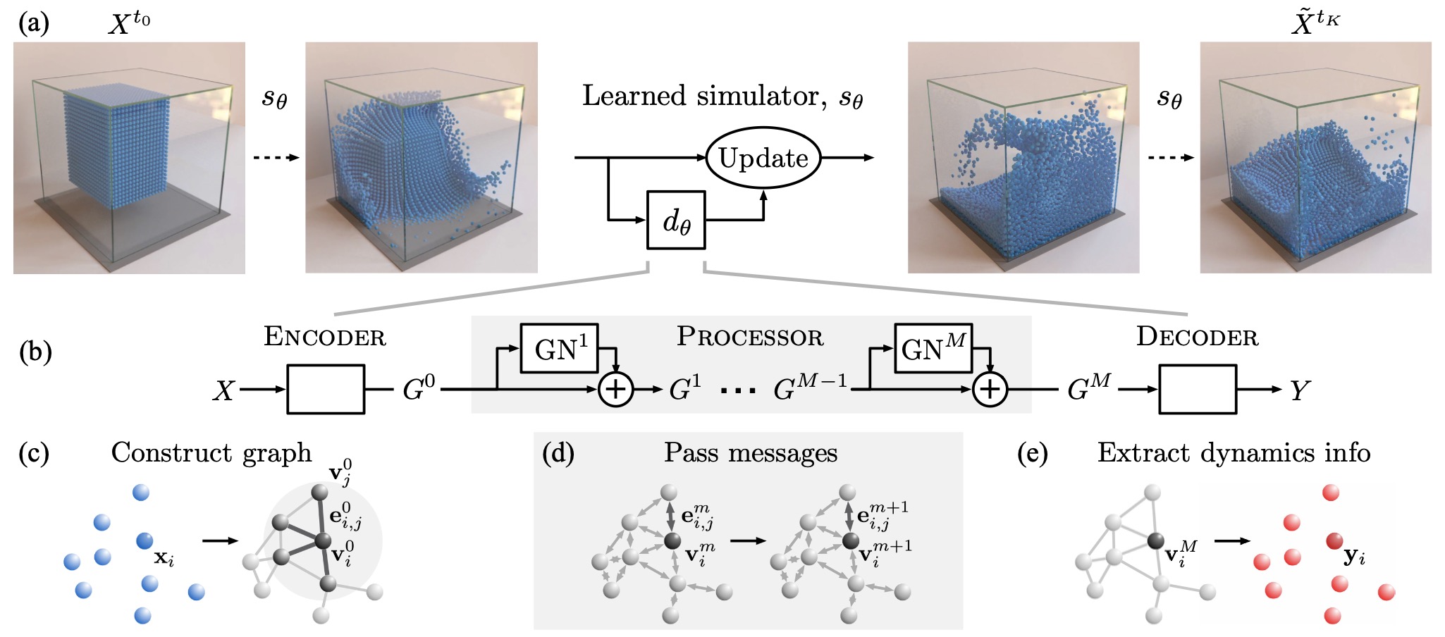
MeshGraphNets and Scientific Simulation
-
Learning Mesh-Based Simulation with Graph Networks by Pfaff et al. (2020) extends graph simulation to mesh-based physical systems, using graph neural networks over adaptive meshes for domains such as aerodynamics, structural mechanics, and cloth simulation.
-
Mesh simulators differ from particle simulators because the graph structure is not only a set of local neighbors; it is a discretization of an underlying physical domain. Nodes represent mesh vertices, edges represent mesh connectivity, and attributes encode geometry, boundary conditions, material state, and dynamic quantities.
-
MeshGraphNets uses both mesh edges and world-space proximity edges, allowing the model to combine discretization-aware local computation with interaction between nearby physical elements. Learning Mesh-Based Simulation with Graph Networks by Pfaff et al. (2020) reports accurate learned rollouts across complex systems and notes that learned mesh simulators can run substantially faster than the numerical solvers used to generate their training data.
-
The following figure (source) shows MeshGraphNets (operating on their SphereDynamic domain), where simulation state is encoded on a mesh graph, processed through message passing, and decoded into updated physical quantities. The model uses an Encode-Process-Decode architecture trained with one-step supervision, and can be applied iteratively to generate long trajectories at inference time. The encoder transforms the input mesh \(M^t\) into a graph, adding extra world-space edges. The processor performs several rounds of message passing along mesh edges and world edges, updating all node and edge embeddings. The decoder extracts the acceleration for each node, which is used to update the mesh to produce \(M^{t+1}\).
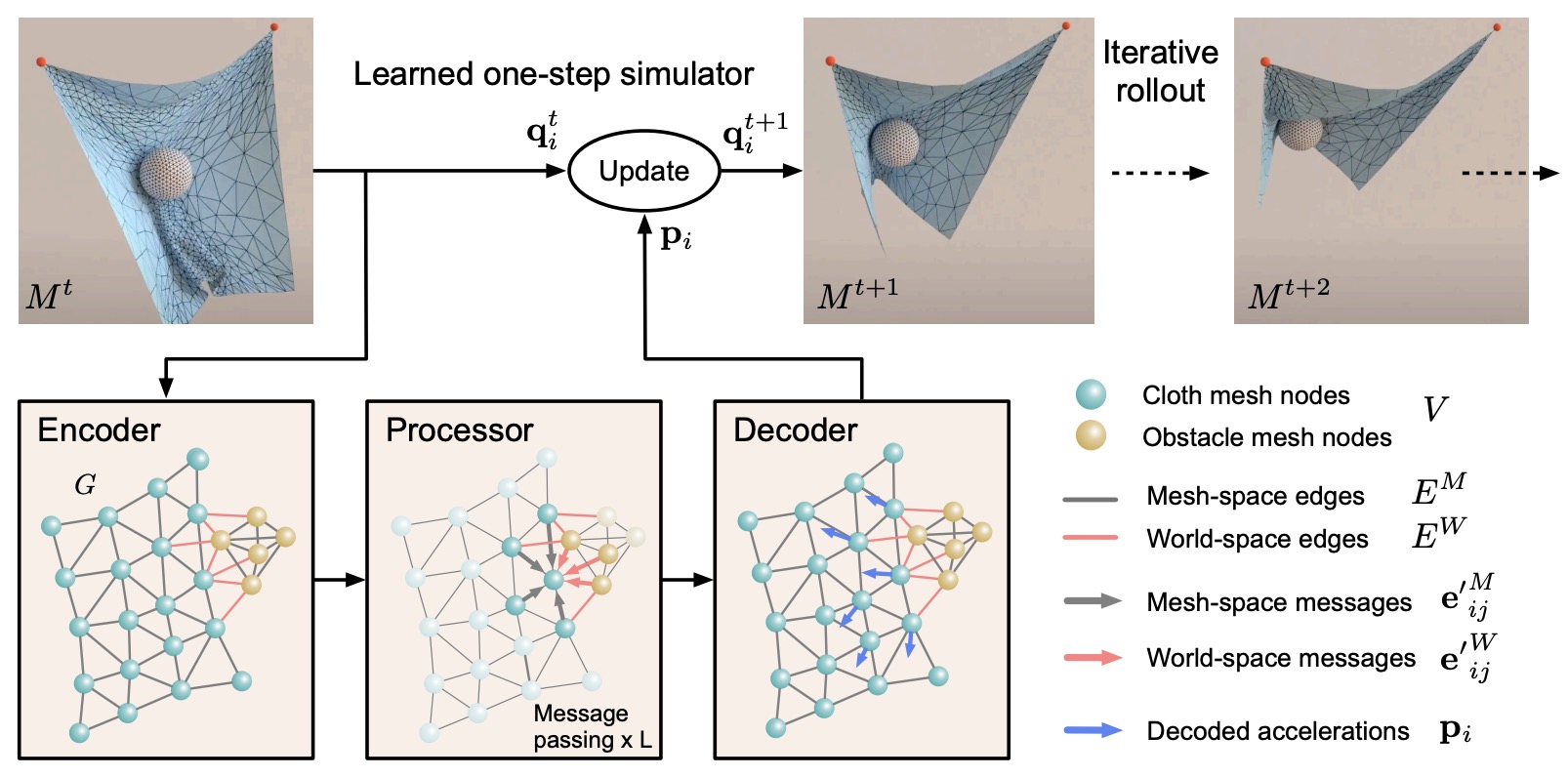
- Mesh-based learned simulators are particularly important for engineering because mesh resolution can adapt to regions requiring precision, such as boundary layers in fluid flow, contact regions in cloth, and stress concentrations in deformable structures. This makes them a natural simulator-world-model paradigm for scientific and industrial domains.
Implementation Pattern for Learned Physical Simulators
-
A learned physical simulator generally follows a dense implementation pattern: choose a state representation that exposes relevant physical variables, construct a graph from objects, particles, or mesh elements, encode node and edge attributes with neural networks, perform multiple message-passing steps to approximate local interactions, decode accelerations or state deltas, integrate the predicted dynamics through time, and train on one-step or multi-step prediction losses while adding noise or rollout training to reduce compounding error.
-
A generic one-step objective is:
-
A rollout objective is:
\[\mathcal{L}_{\text{rollout}} =\sum_{k=1}^{H} \left| \hat{z}_{t+k}-z_{t+k} \right|_2^2\]- where:
-
The rollout loss is more expensive but better aligned with simulator use, because downstream planners care about long-horizon accuracy rather than isolated one-step predictions.
Error Accumulation and Stabilization
-
Learned simulators face the same compounding-error problem as interactive renderers, but state-space errors are often more consequential. A small velocity error can lead to large position drift; a small contact error can change the outcome of a collision; a small pressure error can destabilize a fluid rollout.
-
Practical stabilization methods include training with corrupted inputs so the model learns to recover from off-manifold states, adding multi-step rollout losses so the model is exposed to its own predictions, enforcing conservation-inspired constraints when known, normalizing state variables and edge features to improve optimization, and using graph locality to preserve physical inductive bias. Learning to Simulate Complex Physics with Graph Networks by Sanchez-Gonzalez et al. (2020) identifies message-passing depth and training-time noise corruption as major determinants of long-term simulation quality. ([arXiv][5])
Relationship to Renderer Models and JEPA
- Learned physical simulators differ from renderer world models in the object they optimize. Renderers produce observations:
- Simulators produce state:
-
JEPA sits close to the simulator paradigm because it also predicts latent state rather than reconstructing pixels, but graph simulators are usually more explicitly structured: their state is object, particle, or mesh based, and their dynamics are organized around relations. This makes graph simulators highly interpretable and physically grounded, while JEPA-style latent simulators are often more scalable to raw sensory data and less dependent on manually specified state variables.
-
A mature world-model stack may combine these approaches: a perception system or JEPA encoder constructs latent state from observations, a graph simulator rolls forward structured dynamics, and a renderer decodes selected states into visual observations for inspection, training, or human interaction.
Simulator World Models: Evaluation, Interfaces, and Integration
Simulator Interfaces
-
A simulator world model should expose a state interface that can be queried, updated, and evaluated. Unlike renderer models, which produce observations, simulator models should preserve variables that matter for future prediction:
\[z_t = {x_t, v_t, m, r, c, \rho, \mathcal{G}_t}\]- where \(x_t\) may denote positions, \(v_t\) velocities, \(m\) masses, \(r\) object relations, \(c\) contacts, \(\rho\) material parameters, and \(\mathcal{G}_t\) graph structure. The exact state depends on the domain: NeRF-style models expose continuous radiance fields, 3D Gaussian Splatting exposes explicit Gaussian primitives, graph simulators expose particles or objects, and mesh simulators expose discretized physical fields.
-
NeRF by Mildenhall et al. (2020) exposes a continuous 5D radiance field useful for view synthesis, while 3D Gaussian Splatting by Kerbl et al. (2023) exposes editable spatial primitives that make real-time rendering more practical. Learning to Simulate Complex Physics with Graph Networks by Sanchez-Gonzalez et al. (2020) exposes particle states as graph nodes and uses message passing to predict physical evolution.
State Accuracy and Rollout Accuracy
- Simulator evaluation should distinguish one-step accuracy from rollout accuracy. One-step prediction measures whether the model can estimate the immediate next state:
-
Rollout accuracy measures whether the simulator remains stable under its own predictions:
\[\mathcal{L}_{\text{rollout}} = \sum_{k=1}^{H} \left| \hat{z}_{t+k}-z_{t+k} \right|_2^2\]-
where:
\[\hat{z}_{t+k+1}=F_\theta(\hat{z}_{t+k},a_{t+k})\]
-
-
This distinction is crucial because a model can have low one-step error yet fail when rolled out for many steps. Learning to Simulate Complex Physics with Graph Networks by Sanchez-Gonzalez et al. (2020) emphasizes long-horizon rollout robustness and shows that training-time noise corruption helps the model recover from off-distribution prediction errors.
Physical Plausibility
-
A simulator should satisfy physical plausibility constraints whenever the domain has known structure. These constraints may include conservation of mass, bounded energy drift, collision consistency, material constraints, mesh validity, and contact stability. In learned simulators, these constraints can be enforced explicitly through the architecture, softly through regularization, or implicitly through training data.
-
A generic physically regularized loss is:
- Interaction Networks by Battaglia et al. (2016) showed that object-relation inductive bias helps neural simulators reason about physical systems, while Learning Mesh-Based Simulation with Graph Networks by Pfaff et al. (2020) uses mesh structure to model physical systems such as cloth, aerodynamics, and structural mechanics.
Editability and Counterfactual Validity
-
A simulator should support counterfactual changes. If the mass of an object changes, the model should predict a different trajectory. If a force is applied, the model should update the future state accordingly. If a camera viewpoint changes, a spatial simulator should render the same underlying scene from the new view.
-
Counterfactual validity can be expressed as:
- The simulator should respond consistently to \(\delta\). Learning to See Physics via Visual De-animation by Wu et al. (2017) is important here because it recovers physical world state from vision and then uses physics and graphics engines for prediction and reasoning, making counterfactual physical inference part of the simulator interface.
Rendering as a Diagnostic, Not the Whole Objective
- Many simulator world models include a renderer:
-
Rendering is useful because observations provide supervision and allow humans to inspect predicted states. However, a good rendered image is not sufficient proof of a good simulator. The latent state may still be geometrically inconsistent, physically invalid, or unstable under intervention.
-
This is the key distinction from renderer world models. A renderer can be evaluated by visual quality, but a simulator must be evaluated by whether its internal state remains valid. DreamFusion by Poole et al. (2022) illustrates this boundary: a 2D diffusion prior supervises a 3D representation through rendered views, but the target object is a 3D state that can be viewed, relit, and composed into 3D environments.
Integration with Planners
- Simulator world models become decision-relevant when a planner can use them to evaluate possible actions. Given a learned dynamics model \(\hat{z}_{t+1}=F_\theta(z_t,a_t)\), a planner can search for an action sequence that minimizes a goal-conditioned cost:
-
The simulator need not render every candidate future. It only needs to provide a reliable state rollout and a cost-relevant representation. This is why simulator world models are often more efficient than renderer world models for control.
-
A dense evaluation criterion for simulator-planner integration should measure whether simulated trajectories preserve goal-relevant state, whether the planner’s selected actions transfer to the real or target environment, whether rollout errors compound under closed-loop replanning, and whether the simulator supports interventions outside the exact training distribution.
Relationship to JEPA
- Simulator world models and JEPA world models are closely related because both prioritize state prediction over pixel reconstruction. The difference is the explicitness of the state. Graph simulators and mesh simulators represent state as objects, particles, relations, or mesh fields. JEPA represents state as learned embeddings:
- This makes JEPA more scalable to unstructured sensory data, but often less inspectable than object-centric or mesh-based simulators. A strong world-model architecture may combine both approaches: JEPA-style encoders can learn compact predictive representations from raw video, while graph or mesh simulators can impose relational and physical structure where explicit state is available.
Planner World Models
Latent Imagination and Model-Based Control
-
Planner world models are systems whose primary output is action. A renderer predicts observations, a simulator predicts state, and a planner chooses interventions that are expected to achieve a goal. In learned world-model planning, the agent first learns a predictive model of the environment, then uses that model to evaluate candidate futures:
\[a_{t:t+H}^{*} =\arg\max_{a_{t:t+H}} \mathbb{E} \left[ \sum_{k=0}^{H} \gamma^k r(\hat{z}_{t+k},a_{t+k}) \right]\]- where \(\hat{z}_{t+k}\) is a predicted latent state and \(H\) is the planning horizon. World Models by Ha and Schmidhuber (2018) established the neural world-model framing in which an agent learns compressed spatial and temporal representations, then trains a compact controller using those learned features.
-
The following figure (source) shows the World Models pipeline, which consists of three components that work closely together: Vision (V), Memory (M), and Controller (C). Visual observations are compressed by a VAE, temporal dynamics are modeled by an MDN-RNN, and a compact controller acts using the learned latent state.
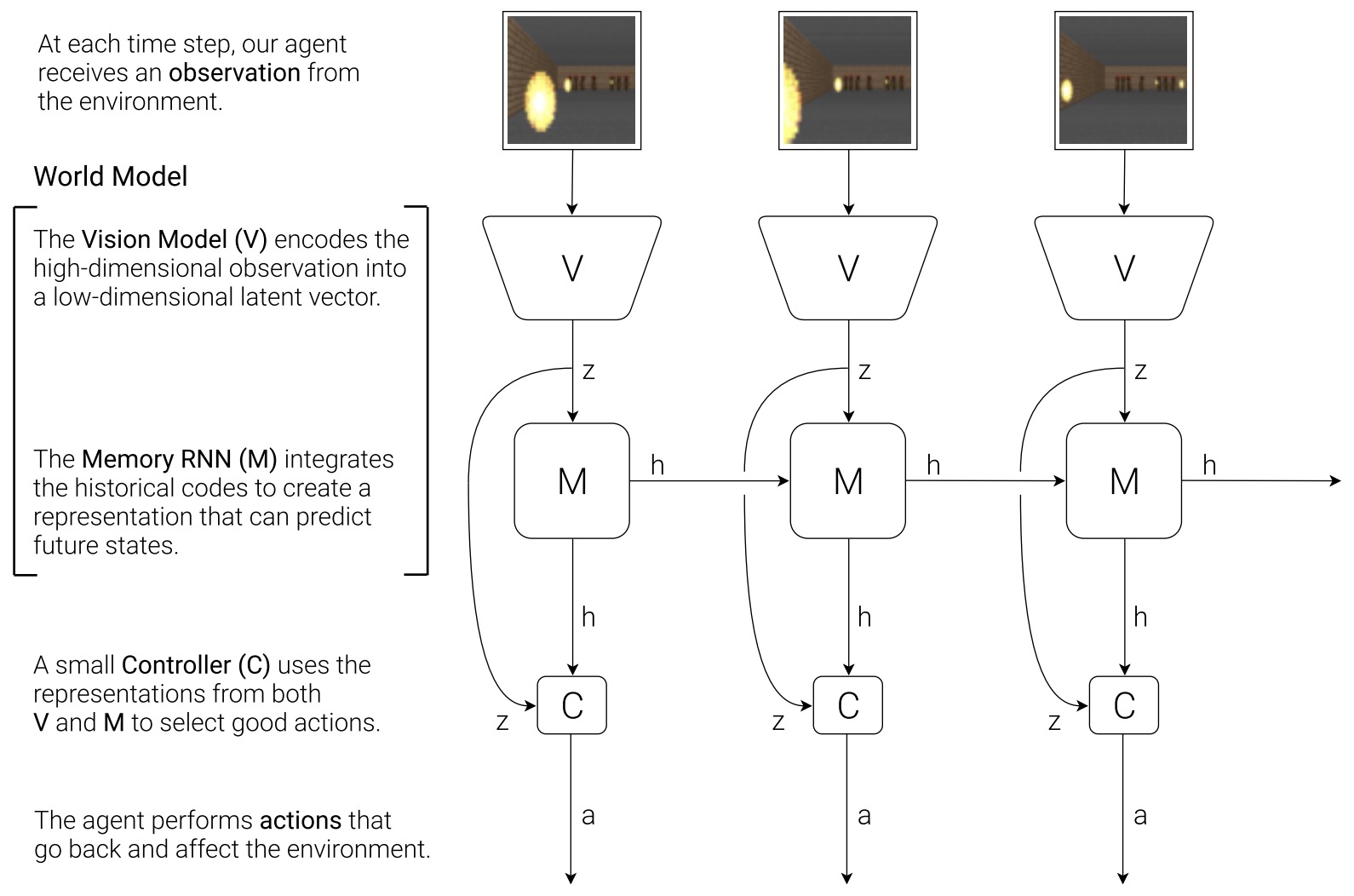
Planning from Pixels with Latent Dynamics
-
The central challenge in planner world models is that raw observations are too high-dimensional for direct planning. A planner should not search over pixels; it should search over compact latent states that preserve reward-relevant dynamics.
-
Learning Latent Dynamics for Planning from Pixels by Hafner et al. (2019) introduced PlaNet, a model-based agent that learns a recurrent state-space model from images and chooses actions through online planning in latent space.
-
PlaNet uses a latent dynamics model with deterministic and stochastic components:
-
The deterministic state \(h_t\) preserves recurrent memory, while the stochastic state \(z_t\) represents uncertainty and partial observability. Planning then uses model predictive control, commonly with the cross-entropy method, to sample candidate action sequences, roll them forward in latent space, score predicted rewards, and execute the first action before replanning.
-
The following figure (source) shows PlaNet learning latent dynamics from image observations and using online planning in compact latent space to choose actions. Specifically, it shows the image-based control domains used in their experiments. The images show agent observations before downscaling to \(64 \times 64 \times 3\) pixels. (a) The cartpole swingup task has a fixed camera so the cart can move out of sight. (b) The reacher task has only a sparse reward. (c) The cheetah running task includes both contacts and a larger number of joints. (d) The finger spinning task includes contacts between the finger and the object. (e) The cup task has a sparse reward that is only given once the ball is caught. (f) The walker task requires balance and predicting difficult interactions with the ground when the robot is lying down.

- A compact implementation pattern is:
belief = encoder.observe(history)
for iteration in range(num_cem_iters):
    action_sequences = sample_action_sequences(distribution)
    imagined_states = world_model.rollout(belief, action_sequences)
    returns = reward_model(imagined_states).sum(dim="time")
    distribution = refit_to_elite_sequences(action_sequences, returns)
action = distribution.mean[0]
- The important design choice is that planning happens inside the learned latent model, not in observation space. This is why PlaNet belongs to the planner branch even though it learns a simulator internally: the learned simulator exists to support action selection.
Latent Imagination and Policy Learning
-
Online planning can be computationally expensive because it repeatedly samples and evaluates action sequences at decision time. Dreamer shifts the emphasis from online search to policy learning inside imagined latent trajectories.
-
Dream to Control: Learning Behaviors by Latent Imagination by Hafner et al. (2019) introduced Dreamer, which learns long-horizon behaviors by backpropagating value estimates through trajectories imagined in the compact latent state space of a learned world model.
-
Dreamer learns three coupled components:
-
The actor is trained on imagined rollouts rather than only real environment transitions:
\[\mathcal{L}_{\text{actor}} =-\mathbb{E} \left[ \sum_{t=1}^{H} V_\lambda(z_t) \right]\]- where \(V_\lambda\) is a bootstrapped return estimate computed from imagined rewards and critic values. Dream to Control by Hafner et al. (2019) is central because it shows that a planner world model can become a behavior-learning system: the model generates imagined futures, and the policy improves by differentiating through those futures.
-
The following figure (source) shows Dreamer learning a world model from experience and learning behaviors by propagating value estimates through imagined latent trajectories.
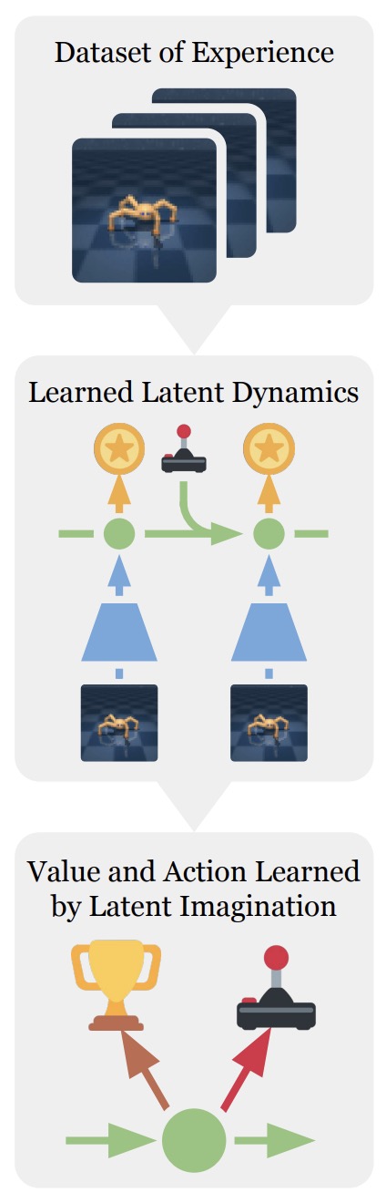
Uncertainty-Aware Planning with Probabilistic Dynamics
-
Planning becomes risky when the learned model is uncertain. If a planner exploits model errors, it may choose actions that look good inside the model but fail in the real environment. Probabilistic dynamics models address this by representing uncertainty over transitions.
-
PETS: Deep Reinforcement Learning in a Handful of Trials using Probabilistic Dynamics Models by Chua et al. (2018) combines probabilistic neural network ensembles with trajectory sampling, enabling model predictive control that accounts for epistemic and aleatoric uncertainty.
-
A probabilistic ensemble dynamics model can be written as:
\[p_\theta(s_{t+1}\mid s_t,a_t) =\frac{1}{M} \sum_{m=1}^{M} p_{\theta_m}(s_{t+1}\mid s_t,a_t)\]-
where different ensemble members represent model uncertainty. Planning then evaluates action sequences under sampled futures rather than a single deterministic rollout:
\[J(a_{t:t+H}) =\mathbb{E}_{p_\theta} \left[ \sum_{k=0}^{H} r(s_{t+k},a_{t+k}) \right]\]
-
-
This makes PETS a useful bridge between simulator and planner paradigms: the simulator is not only predictive, but also uncertainty-aware, and the planner uses that uncertainty when choosing actions.
Why Planner World Models Matter
- Planner world models are the point where world modeling becomes agency. A renderer can show possible futures, and a simulator can roll forward state, but a planner decides what to do. The planning objective converts prediction into intervention:
- A practical planning world model should therefore satisfy a dense set of requirements: it should learn compact states that preserve reward-relevant information, predict futures accurately enough over the planner’s horizon, represent uncertainty when the future is ambiguous, avoid exploiting model errors, support efficient candidate-action evaluation, and improve policies using imagined experience rather than only real interaction.
Search, Task-Oriented Latent Models, and Scalable Control
Planning-Relevant Models Rather than Complete Simulators
- A planning world model does not need to reconstruct every aspect of the environment. It needs to preserve the aspects of the future that change the ranking of candidate actions. This motivates a task-oriented objective:
-
The learned state \(z_t\) is valuable when it supports accurate reward, value, and action evaluation, even if it cannot reconstruct the original observation. Mastering Atari, Go, Chess and Shogi by Planning with a Learned Model by Schrittwieser et al. (2020) formalized this principle in MuZero: its model predicts reward, policy, and value quantities relevant to search, without requiring observation reconstruction or access to environment rules.
-
This distinction separates planning world models from generative simulators. A generative model is trained to explain observations:
- A planning model is trained to preserve decision-relevant quantities:
- The second objective can be substantially easier because it ignores visual details, stochastic nuisance variables, and environmental structure that do not affect the agent’s decision. MuZero explicitly learns a hidden state that is free to represent whatever internal structure best supports accurate planning, rather than matching a true environment state or reconstructing observations.
MuZero and Search over Learned Latent States
-
MuZero combines a learned latent dynamics model with Monte Carlo Tree Search. It contains a representation function, a dynamics function, and a prediction function:
\[s_t^0=h_\theta(o_{1:t})\] \[r_t^k,s_t^k=g_\theta(s_t^{k-1},a_t^k)\] \[p_t^k,v_t^k=f_\theta(s_t^k)\]- where \(h_\theta\) maps observation history into a latent root state, \(g_\theta\) predicts the next latent state and immediate reward under a hypothetical action, and \(f_\theta\) predicts policy logits and value. Mastering Atari, Go, Chess and Shogi by Planning with a Learned Model by Schrittwieser et al. (2020) shows that a learned planning model can support superhuman performance in Go, chess, and shogi while also achieving strong Atari results without being given game rules.
-
The planning loop evaluates a search tree using learned priors and values:
\[a_t^*=\arg\max_a N(s_t,a)\]-
where \(N(s_t,a)\) is the visit count assigned by search. A typical selection score combines action value, exploration pressure, and policy prior:
\[U(s,a) =Q(s,a) + c_{\text{puct}} P(s,a) \frac{\sqrt{\sum_b N(s,b)}}{1+N(s,a)}\]
-
-
The central insight is that the model need not simulate observations. It only needs to generate latent transitions that let search compare action branches. This is particularly effective in discrete-action domains, where tree search can efficiently expand and revisit promising branches.
-
The following figure (source) shows MuZero’s learned planning model, where an observation is encoded into a hidden state, hypothetical actions are applied through recurrent latent dynamics, and each latent state predicts reward, policy, and value for tree search. Specifically, it shows planning, acting, and training with a learned model. (A) How MuZero uses its model to plan. The model consists of three connected components for representation, dynamics and prediction. Given a previous hidden state \(s^{k-1}\) and a candidate action \(a^k\), the dynamics function \(g\) produces an immediate reward \(r^k\) and a new hidden state \(s^k\). The policy \(p^k\) and value function \(v^k\) are computed from the hidden state \(s^k\) by a prediction function \(f\). The initial hidden state \(s^0\) is obtained by passing the past observations (e.g. the Go board or Atari screen) into a representation function \(h\). (B) How MuZero acts in the environment. A Monte-Carlo Tree Search is performed at each timestep \(t\), as described in A . An action \(a_{t+1}\) is sampled from the search policy \(\pi_t\), which is proportional to the visit count for each action from the root node. The environment receives the action and generates a new observation \(o_{t+1}\) and reward \(u_{t+1}\). At the end of the episode the trajectory data is stored into a replay buffer. (C) How MuZero trains its model. A trajectory is sampled from the replay buffer. For the initial step, the representation function \(h\) receives as input the past observations \(o_1, \ldots, o_t\) from the selected trajectory. The model is subsequently unrolled recurrently for \(K\) steps. At each step \(k\), the dynamics function \(g\) receives as input the hidden state \(s^{k-1}\) from the previous step and the real action \(a_{t+k}\). The parameters of the representation, dynamics and prediction functions are jointly trained, end-to-end by backpropagation-through-time, to predict three quantities: the policy \(\mathbf{p}^k \approx \pi_{t+k}\), value function \(v^k \approx z_{t+k}\), and reward \(r_{t+k} \approx u_{t+k}\), where \(z_{t+k}\) is a sample return: either the final reward (board games) or \(n\)-step return (Atari).
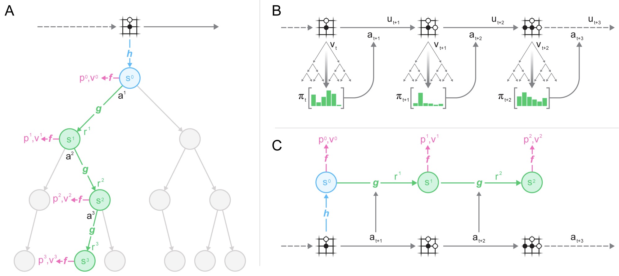
Model Predictive Control with Task-Oriented Latent Dynamics
-
Continuous-control planning often cannot enumerate actions through tree search. Instead, it samples and refines candidate action trajectories. Temporal Difference Learning for Model Predictive Control by Hansen et al. (2022) introduced TD-MPC, which combines short-horizon trajectory optimization in a task-oriented latent model with a learned terminal value function.
-
TD-MPC learns an encoder, latent transition model, reward model, value function, and policy prior:
-
The planner evaluates an action sequence using short-horizon model rollouts and a terminal value estimate:
\[\phi(\Gamma) =\sum_{k=0}^{H-1} \gamma^k R_\theta(z_k,a_k) + \gamma^H Q_\theta(z_H,a_H)\]-
where:
\[z_{k+1}=d_\theta(z_k,a_k)\]
-
-
This hybrid objective is important because it reduces the need for very long model rollouts. The latent model handles local trajectory optimization, while the terminal value function estimates long-range consequences beyond the planning horizon. Temporal Difference Learning for Model Predictive Control by Hansen et al. (2022) argues that this task-oriented formulation avoids spending model capacity on irrelevant visual details while preserving the quantities required for continuous control.
-
The following figure (source) shows TD-MPC combining a task-oriented latent dynamics model, reward prediction, terminal value estimation, policy guidance, and model predictive trajectory optimization. (Top) A framework for MPC is presented using a task-oriented latent dynamics model and value function learned jointly by temporal difference learning. We perform trajectory optimization over model rollouts and use the value function for long-term return estimates. (Bottom) Episode return of our method, SAC, and MPC with a ground-truth simulator on challenging, high dimensional Humanoid and Dog tasks. Mean of 5 runs; shaded areas are 95% confidence intervals.
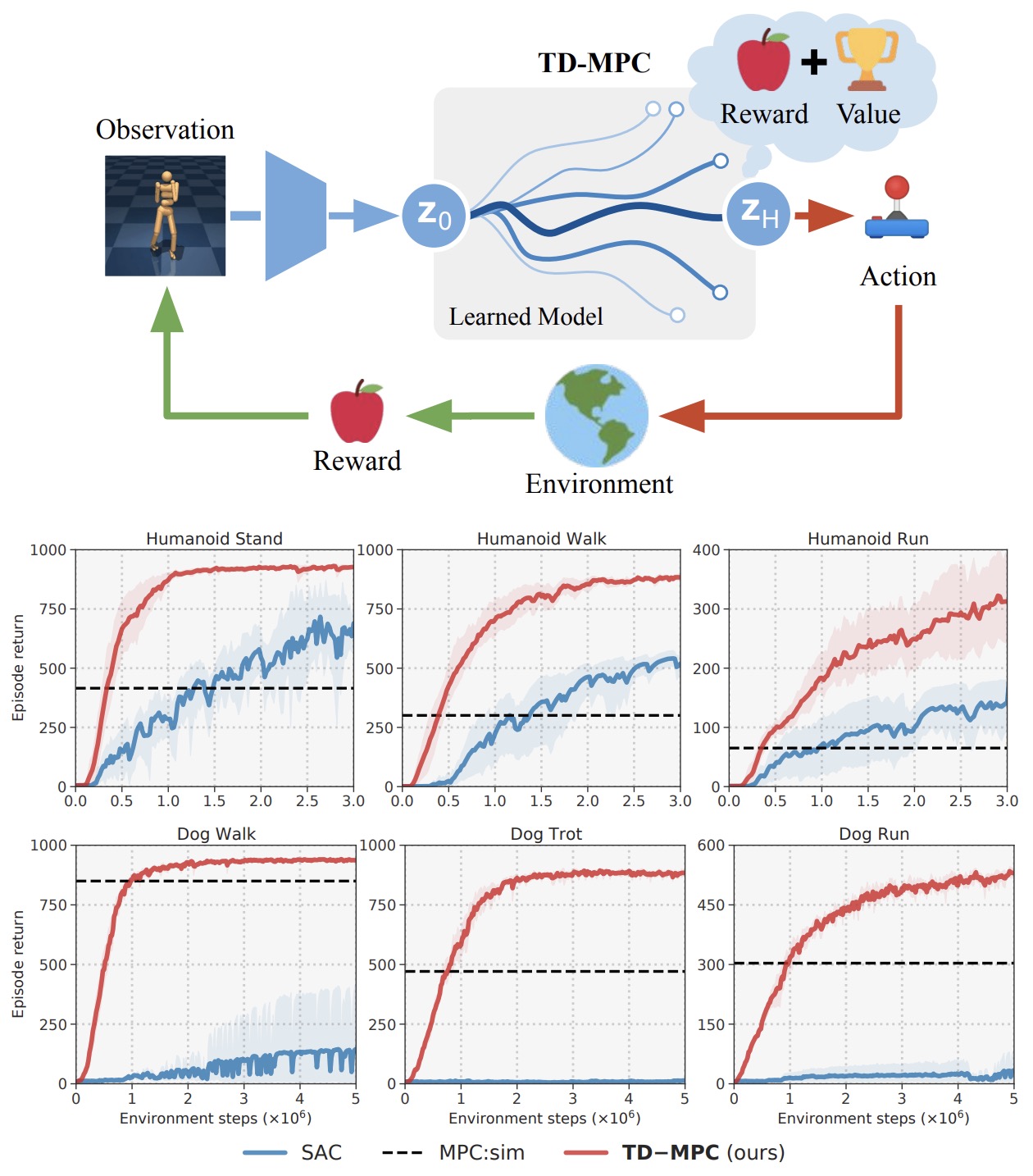
Sampling-Based Trajectory Optimization
- TD-MPC uses Model Predictive Path Integral control to optimize continuous action sequences. The planner samples candidate trajectories from a time-indexed Gaussian distribution:
-
Each sampled trajectory is rolled out in latent space and scored by predicted return. The mean and variance are then updated from high-scoring samples:
\[\mu^{j} =\frac{ \sum_{i=1}^{K} \Omega_i \Gamma_i^{*} }{ \sum_{i=1}^{K} \Omega_i }\] \[\sigma^{j} =\sqrt{ \frac{ \sum_{i=1}^{K} \Omega_i \left( \Gamma_i^{*}-\mu^j \right)^2 }{ \sum_{i=1}^{K} \Omega_i } }\]- where \(\Omega_i\) weights elite trajectories according to predicted return. Temporal Difference Learning for Model Predictive Control by Hansen et al. (2022) uses this sampling-based planning procedure together with a learned policy prior, allowing planning to focus on locally promising trajectories rather than uniformly exploring the full continuous action space.
-
This planning mechanism illustrates an important distinction between MuZero and TD-MPC. MuZero searches discrete action trees using MCTS. TD-MPC searches continuous action sequences using trajectory sampling and distribution refinement. Both rely on learned latent models, but their planning algorithms match different action-space structures.
Scaling Task-Oriented Planning with TD-MPC2
-
TD-MPC2: Scalable, Robust World Models for Continuous Control by Hansen et al. (2024) extends task-oriented latent planning toward multi-task and multi-domain control, using a single set of hyperparameters across diverse continuous-control tasks.
-
TD-MPC2 retains the basic structure of latent model predictive control but strengthens representation normalization, reward and value learning, policy priors, and multi-task conditioning. Its latent state uses SimNorm, a normalization mechanism that biases representations toward sparse, bounded structure:
-
The model additionally uses task embeddings:
\[z_t=e_\theta(o_t,\tau)\]- where \(\tau\) is a learned task representation that conditions the encoder, dynamics model, reward model, value functions, and policy. This enables a single agent to operate across tasks with different embodiments, observation spaces, and action spaces. TD-MPC2 by Hansen et al. (2024) reports scaling a single 317-million-parameter agent across 80 continuous-control tasks and evaluates a shared configuration across 104 tasks.
-
The following figure (source) shows the TD-MPC2 architecture. Observations s are encoded into their (normalized) latent representation \(z\). The model then recurrently predicts actions \(a\mathbin{\text{\^}}\), rewards \(r\mathbin{\text{\^}}\), and terminal values \(q\mathbin{\text{\^}}\), without decoding future observations.
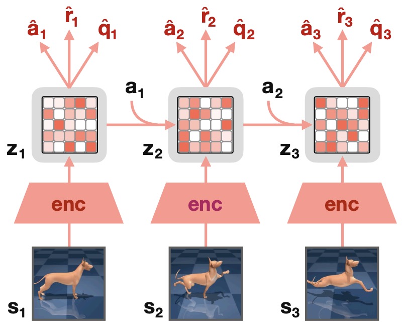
- TD-MPC2 also revises the reward and value objectives by using discretized regression in a transformed reward space, reducing sensitivity to task-dependent reward magnitudes. This matters for multi-task planning because raw reward scales can vary sharply across domains, destabilizing a shared model.
Discrete Latent Planning and DreamerV2
-
Mastering Atari with Discrete World Models by Hafner et al. (2021) introduced DreamerV2, which uses discrete stochastic latent variables to improve world-model learning and trains behavior entirely through imagined trajectories.
-
DreamerV2 represents latent state with categorical variables:
\[z_t =\left[ z_t^{(1)}, z_t^{(2)}, \dots, z_t^{(K)} \right]\]- where each component is sampled from a categorical distribution. Discrete latent variables can make the model less sensitive to small continuous-state drift and improve its ability to represent multimodal futures. Mastering Atari with Discrete World Models by Hafner et al. (2021) reports that discrete latents and KL balancing are important contributors to its Atari performance, while the learned world model supports policy optimization entirely in imagined experience.
-
The planning significance is that DreamerV2 trades explicit online search for extensive latent policy optimization. It learns a world model, imagines many trajectories in parallel, updates actor and critic networks from those trajectories, and executes the learned policy in the environment. This makes it especially useful when decision latency must remain low at inference time.
Planning Architecture Trade-offs
-
Planner world models can be organized by how they allocate computation. MuZero spends substantial test-time computation on search, making it suitable for discrete domains with deep combinatorial structure. TD-MPC spends test-time computation on short-horizon continuous trajectory optimization, making it suitable for continuous control and receding-horizon decision making. Dreamer-style agents spend more computation during training to improve an amortized policy, making inference efficient. PETS spends computation on uncertainty-aware trajectory sampling, making it useful when model uncertainty is central.
-
A practical architecture choice should consider the action space, planning horizon, environment stochasticity, model uncertainty, inference latency, and whether task-relevant value functions can compensate for limited rollout horizons. The key design principle remains:
Evaluation and Failure Modes
Planning Evaluation Should Match the Decision Loop
-
A planner world model should be evaluated by the quality of the actions it produces, not only by the accuracy of its predictions. A learned model can have plausible rollouts but still produce poor actions if its errors affect reward-relevant variables, if its value estimates are miscalibrated, or if the planner exploits model inaccuracies.
-
The relevant objective is closed-loop return:
- rather than only one-step prediction loss:
- TD-MPC2: Scalable, Robust World Models for Continuous Control by Hansen et al. (2024) evaluates planning across 104 continuous-control tasks and shows that robust task-oriented latent models can outperform strong model-free and model-based baselines under a shared hyperparameter setting.
Model Exploitation and Reward Misgeneralization
- A planner searches for actions that maximize predicted value. If the world model is wrong, the planner may exploit the error. This is model exploitation:
-
The risk is greatest when the planner evaluates out-of-distribution action sequences, when rollouts are long, or when the value model extrapolates beyond its training support. PETS: Deep Reinforcement Learning in a Handful of Trials using Probabilistic Dynamics Models by Chua et al. (2018) addresses this by using probabilistic ensembles and trajectory sampling, so the planner reasons over uncertainty rather than trusting a single deterministic model.
-
A dense evaluation protocol should therefore measure policy return, calibration of uncertainty, sensitivity to out-of-distribution actions, degradation under longer planning horizons, and the gap between predicted and realized returns.
Planning Horizon and Compounding Error
-
Longer planning horizons can improve foresight, but they also amplify model error. If the model’s transition error at each step is \(\epsilon\), then rollout error can grow approximately as:
\[|\hat{z}_{t+H}-z_{t+H}| \leq \sum_{k=0}^{H-1} L^k\epsilon\]- where \(L\) is an effective Lipschitz constant of the learned dynamics. When \(L>1\), errors can grow rapidly.
-
This is why many successful planner world models combine short rollouts with terminal values. Temporal Difference Learning for Model Predictive Control by Hansen et al. (2022) uses short-horizon latent planning with a terminal value function, so the learned model handles local control while the critic estimates long-term return.
-
The following figure (source) shows how TD-MPC performance varies with planning horizon and the number of planning iterations, illustrating the compute-performance trade-off in model predictive control. Specifically, it shows the return of TD-MPC under a variable computational budget on four other tasks from DMControl: Quadruped Run (\(\mathcal{A} \in \mathbb{R}^{12}\)), Fish Swim (\(\mathcal{A} \in \mathbb{R}^5\)), Reacher Hard \(\left(\mathcal{A} \in \mathbb{R}^2\right)\), and Cartpole Swingup Sparse \((\mathcal{A} \in \mathbb{R})\). We evaluate performance of fully trained agents when varying (blue) planning horizon; (green) number of iterations during planning. For completeness, we also include evaluation of the jointly learned policy \(\pi_\theta\), as well as the default setting of 6 iterations and a horizon of 5 used during training. Higher values require more compute. Mean of 5 runs.
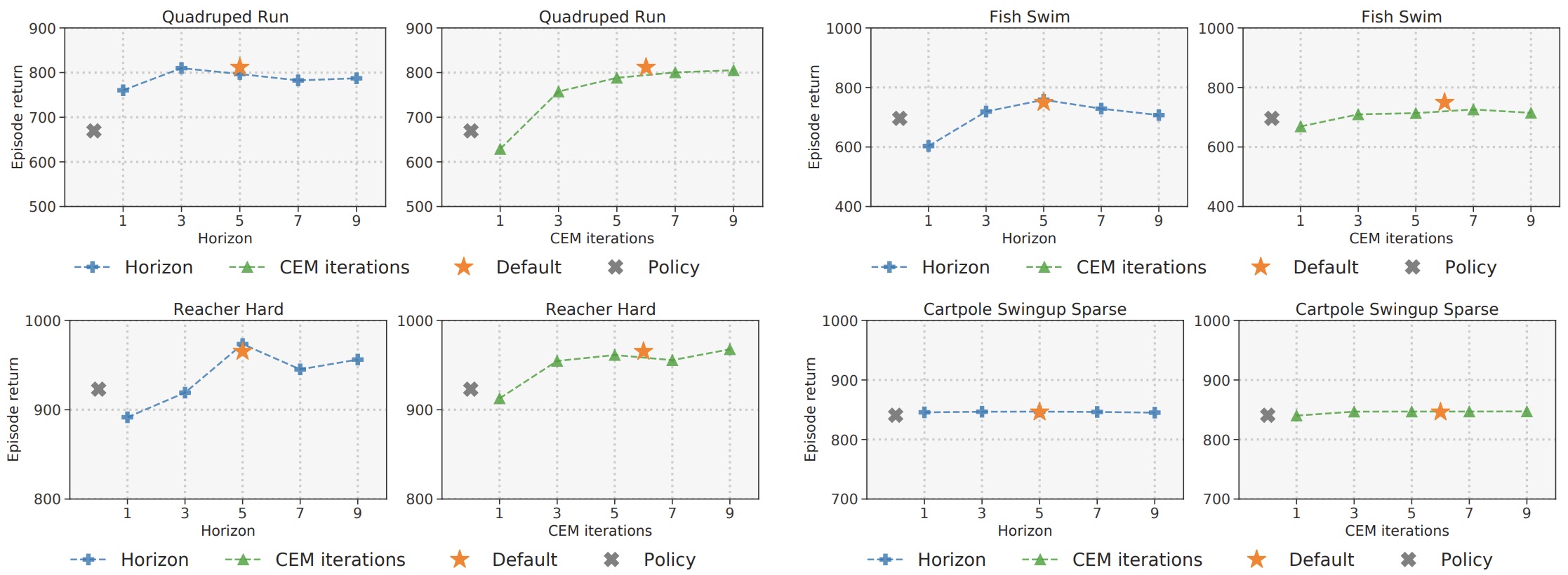
Online Search versus Amortized Planning
-
Planner world models allocate computation in different places. Online search methods spend computation at decision time; amortized methods spend more computation during training so that inference is fast.
-
MuZero performs online tree search over a learned latent model:
- Dreamer trains an actor to amortize planning into a policy:
- TD-MPC combines both by using a learned policy prior to guide test-time trajectory optimization:
- Mastering Atari, Go, Chess and Shogi by Planning with a Learned Model by Schrittwieser et al. (2020) shows the strength of search-based decision making in discrete domains, while Dream to Control by Hafner et al. (2019) shows that behaviors can be learned by backpropagating value estimates through imagined latent trajectories.
Data Efficiency and Imagination Efficiency
- Planner world models improve sample efficiency by reusing experience through imagined futures. A single real transition can train many imagined rollouts:
-
Dreamer-style models are particularly efficient because thousands of latent rollouts can be generated in parallel. Dream to Control by Hafner et al. (2019) emphasizes that compact latent states reduce memory and compute, enabling large numbers of imagined trajectories during training.
-
However, imagination efficiency only helps if imagined trajectories remain useful. If the model predicts wrong rewards or loses state information, additional imagination can amplify bias rather than improve behavior.
Evaluation Criteria for Planner World Models
-
Planner world models should be evaluated by a dense set of criteria: closed-loop return should measure the realized task performance of the actions produced by the model; data efficiency should measure how many real environment interactions are needed to achieve competence; model exploitation resistance should measure whether the planner avoids actions that are only good under model error; compute efficiency should measure the cost of search, rollouts, value estimation, and policy updates; robustness should measure whether performance holds under domain shift, stochasticity, and partial observability; and transfer should measure whether learned dynamics, values, or task embeddings help on unseen tasks.
-
TD-MPC2 by Hansen et al. (2024) is especially relevant for transfer and scale because it trains multi-task world models across multiple domains, embodiments, and action spaces using learned task embeddings and shared hyperparameters.
Integration with Renderer and Simulator World Models
-
Planner world models need not be visually generative, but they benefit from renderers and simulators in different ways. A renderer can provide synthetic observations, human-interpretable rollouts, and visual debugging. A simulator can provide compact state transitions, counterfactual rollouts, and physically meaningful variables. A planner consumes either rendered observations or simulator states to select actions.
-
A combined stack can be written as:
- and optionally:
- This is the natural architecture for a unified world model: renderers make futures visible, simulators make futures computable, and planners make futures actionable.
Relationship to JEPA
- JEPA connects directly to planner world models because it learns latent predictive states without reconstructing observations. A JEPA-style planner can use:
-
This resembles task-oriented planning models such as TD-MPC, but JEPA emphasizes self-supervised latent prediction and collapse avoidance rather than reward-supervised task representation. A strong future planner could combine JEPA pretraining for scalable latent dynamics, task-oriented value learning for decision relevance, and MPC or search for action selection.
-
This completes the planning branch of the primer. The next section should return to Joint-Embedding Predictive Architectures as the latent predictive paradigm that can connect representation learning, simulation, and planning.
Joint-Embedding Predictive Architectures
Overview
-
Joint-Embedding Predictive Architectures (JEPAs) provide a general framework for learning predictive representations by aligning latent embeddings of related signals rather than reconstructing observations. They represent a shift from reconstruction to prediction, from observation space to representation space, and from static inputs to structured predictive tasks. This shift enables models to focus on predictable, semantically meaningful structure while discarding high-entropy, task-irrelevant details, making JEPA a natural foundation for scalable world modeling.
-
In the renderer-simulator-planner taxonomy, JEPA is most naturally a simulator-oriented latent world model: it predicts hidden state structure rather than directly rendering pixels. When the predictor is action-conditioned and paired with a goal objective, JEPA also becomes a substrate for planners. This makes JEPA complementary to renderer-first systems: renderers prioritize what the world should look like, while JEPA-style models prioritize which latent aspects of the world are predictable and useful for downstream reasoning or control. A Functional Taxonomy of World Models clarifies this distinction by separating world models according to whether they output observations, states, or actions.
Core Principle: Prediction in Representation Space
-
At the core of JEPA is the idea that learning should focus on predicting semantically meaningful aspects of a signal rather than reconstructing the signal itself. Given two compatible signals \(x\) and \(y\), for example, two spatial regions of an image or two time steps in a video, JEPA learns:
\[s_x = f_\theta(x), \qquad s_y = f_{\bar{\theta}}(y)\] \[\hat{s}_y = g_\phi(s_x, \xi)\]- where \(\xi\) encodes auxiliary information such as spatial position, masking indices, temporal offsets, or actions.
-
The objective is to align predicted and target embeddings:
- This formulation replaces pixel-level reconstruction with latent prediction, thereby focusing learning on predictable structure. In functional terms, the target is closer to simulated state than rendered observation: the model is trained to predict what should be true in representation space, not necessarily what every pixel should be.
Architectural Components
-
A JEPA system typically consists of three primary modules:
- Context encoder \(f_\theta\): encodes visible or conditioning inputs \(x\).
- Target encoder \(f_{\bar{\theta}}\): encodes target inputs \(y\), often using an exponential moving average (EMA) of the context encoder.
- Predictor \(g_\phi\): maps context representations to predicted target representations.
-
The following figure (source) shows a comparison between joint-embedding, generative, and joint-embedding predictive architectures, illustrating how JEPA predicts embeddings rather than reconstructing signals.
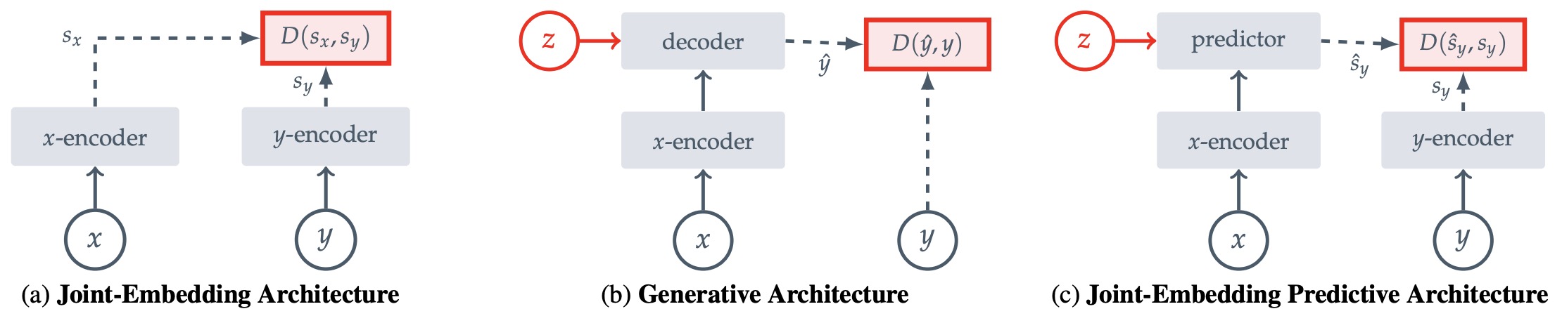
- This architectural asymmetry is critical. The target encoder is typically updated more slowly or frozen, providing stable targets and preventing collapse. Self-Supervised Learning from Images with a Joint-Embedding Predictive Architecture by Assran et al. (2023) uses this setup to train visual representations by predicting masked target-block embeddings rather than reconstructing image pixels.
Masking and Target Selection
-
A defining feature of JEPA is the masking strategy used to construct prediction tasks. Instead of predicting the entire input, JEPA selects target regions and conditions on complementary context.
-
For image-based JEPA:
- Large target blocks encourage semantic prediction.
- Spatially distributed context preserves enough global information for inference.
-
Multiple target regions increase coverage and reduce overfitting to a single local relation.
-
This ensures that prediction cannot be solved using trivial local correlations. Self-Supervised Learning from Images with a Joint-Embedding Predictive Architecture by Assran et al. (2023) emphasizes that target blocks must be sufficiently large and context blocks sufficiently informative to produce semantic representations.
- Formally, let \(M\) denote a masking operator:
-
The model learns to predict the latent representation of \(y\) given \(x\).
-
Target design also distinguishes JEPA-style latent prediction from semantic future-percept prediction. In a JEPA, the target is obtained by encoding a selected region or future observation:
\[s_y = f_{\bar{\theta}}(y)\]-
and the predictor learns to approximate that representation from context. In a semantic predictive model, the target can instead be written abstractly as:
\[z_{t+\Delta} = \Gamma \left( o_{t+\Delta} \right)\]- where \(\Gamma\) extracts a task-relevant semantic future target. Isaac 0.5: Percepts Scale Control by Perceptron (2026) uses automatically constructed future percepts but does not disclose the implementation of \(\Gamma\) or the corresponding semantic loss.
-
-
The distinction changes the invariances learned by the model. JEPA delegates the definition of predictable structure to the learned target encoder and masking strategy, whereas semantic target construction explicitly biases prediction toward object state, spatial relations, affordances, task progress, contact changes, and other task-relevant future semantics. Both avoid full pixel reconstruction, but one learns the target representation end-to-end while the other introduces a semantic bottleneck before prediction. This makes target construction itself a world-model design choice, alongside encoder architecture, masking geometry, and prediction horizon.
Comparison with Other Self-Supervised Objectives
-
JEPA differs from two dominant paradigms:
- Contrastive learning: enforces similarity between augmented views but relies on negative samples.
- Masked reconstruction: predicts missing pixels or tokens directly.
-
JEPA removes both the need for negative samples and the burden of pixel-level reconstruction. It instead enforces predictive consistency in latent space.
-
The distinction can be summarized as:
- Contrastive: \(\text{maximize } \text{sim}(f(x), f(x^+))\)
- Generative: \(\text{minimize } \mid \hat{o} - o \mid\)
- JEPA: \(\text{minimize } \mid \hat{s}_y - s_y \mid\)
-
This distinction maps cleanly onto the functional taxonomy. Generative reconstruction is renderer-like because it optimizes observation fidelity; contrastive learning is representation-oriented but often not explicitly predictive; JEPA is simulator-like because it learns a compact predictive state space.
JEPA, Renderers, Simulators, and Planners
-
JEPA can be positioned precisely within the three functional world-model roles:
- As a renderer alternative: JEPA avoids direct observation generation and therefore does not need to model every high-frequency visual detail.
- As a simulator: JEPA predicts latent state transitions or masked latent states, making it well-suited to compact dynamics modeling.
- As a planner substrate: action-conditioned JEPA can roll forward candidate latent trajectories and score them against a goal.
-
This is important because many systems called world models differ mainly in what they output. A video generator can be a world renderer, a physics engine can be a world simulator, and a policy model can be a world planner. JEPA is most naturally a simulator-style model that can become planner-capable when attached to an action-conditioned predictor and a planning objective. A Functional Taxonomy of World Models makes this distinction explicit by organizing world models by function rather than by architecture.
Avoiding Representation Collapse
- A central challenge in JEPA training is collapse, where the model maps all inputs to a constant embedding:
-
This trivially minimizes the prediction loss if \(\hat{s}_y = c\).
-
JEPA avoids collapse through several mechanisms:
- Architectural asymmetry between context and target encoders
- Stop-gradient or EMA updates for the target encoder
- Masking strategies that enforce non-trivial prediction tasks
-
More recent approaches introduce explicit regularization. LeWorldModel: Stable End-to-End Joint-Embedding Predictive Architecture from Pixels by Maes et al. (2026) enforces Gaussian-distributed latent embeddings using a statistical regularizer, ensuring diversity and preventing collapse.
Temporal and Sequential Extensions
- JEPA naturally extends to sequential data by treating future states as prediction targets:
-
This connects JEPA to latent dynamics modeling and world models.
-
seq-JEPA: Autoregressive Predictive Learning of Invariant-Equivariant World Models by Ghaemi et al. (2026) introduces a sequential formulation where multiple observations and actions are aggregated before predicting the next state, enabling the model to learn both invariant and equivariant representations.
-
DSeq-JEPA: Discriminative Sequential Joint-Embedding Predictive Architecture by He et al. (2026) further refines this by imposing an order over prediction targets, using attention to prioritize semantically important regions.
Multimodal and Cross-Domain Extensions
-
JEPA is not restricted to images. Its formulation applies to any modality where compatible signals can be defined.
- A-JEPA: Joint-Embedding Predictive Architecture Can Listen by Fei et al. (2023) extends JEPA to audio spectrograms, using time-frequency masking and latent prediction.
-
MC-JEPA: A Joint-Embedding Predictive Architecture for Self-Supervised Learning of Motion and Content Features by Bardes et al. (2023) jointly learns motion and semantic features by combining optical flow estimation with latent prediction.
- These extensions demonstrate that JEPA is a modality-agnostic framework for predictive representation learning.
From Representation Learning to World Modeling
-
JEPA becomes a world model when:
- The inputs \(x\) and \(y\) correspond to temporally related observations
- The predictor incorporates action or temporal information
- The latent space supports planning or reasoning tasks
-
In this setting, JEPA learns a predictive latent space \(z_{t+1} \approx g_\phi(z_t, a_t)\) without reconstructing observations. This makes it computationally efficient and aligned with downstream control objectives.
-
V-JEPA 2: Self-Supervised Video Models Enable Understanding, Prediction and Planning by Assran et al. (2025) demonstrates that such representations can scale to internet video and support planning after limited action-conditioned training.
-
From the functional-taxonomy perspective, this is the point where JEPA moves from representation learning into simulator and planner territory: latent predictions provide the simulated future, and action-conditioned rollouts provide the substrate for choosing interventions.
-
The next section focuses specifically on I-JEPA, detailing its design choices, masking strategy, and implementation at scale.
Image-Based Joint-Embedding Predictive Architecture (I-JEPA)
-
I-JEPA represents the first large-scale instantiation of the JEPA framework for visual representation learning. It is designed to learn high-level semantic features from images by predicting latent representations of masked regions using visible context, without relying on handcrafted augmentations or pixel-level reconstruction.
-
In the functional taxonomy of world models, I-JEPA is not yet a complete embodied world model because it does not model actions or temporal dynamics. It is best understood as a representation-learning substrate for simulator-style world models: it learns compact latent structure that later video, object-centric, or action-conditioned systems can use for prediction and planning. A Functional Taxonomy of World Models is useful here because it separates latent state modeling from rendering and planning, clarifying why an image-only model can still be foundational for later world-model systems.
Design Motivation
-
Prior self-supervised approaches in vision fall into two categories:
- Invariance-based methods such as contrastive learning, which rely on augmentations to enforce representation similarity.
- Generative methods such as masked autoencoders, which reconstruct missing pixels or tokens.
-
I-JEPA addresses limitations of both. It avoids augmentation-induced biases and does not require reconstructing high-frequency image details. Instead, it focuses on predicting only the predictable and semantically meaningful aspects of the image. Self-Supervised Learning from Images with a Joint-Embedding Predictive Architecture by Assran et al. (2023) shows that representation-space prediction can produce semantic visual features without handcrafted view augmentations.
-
This design aligns with the hypothesis that intelligent systems learn by predicting the outcomes of partial observations rather than reconstructing full sensory inputs.
Architecture
-
I-JEPA consists of three main components:
- Context encoder \(f_\theta\): processes visible image regions.
- Target encoder \(f_{\bar{\theta}}\): processes masked target regions, typically updated via exponential moving average (EMA).
- Predictor \(g_\phi\): maps context representations to predicted target representations.
-
The model operates entirely in latent space. Given an image \(o\), a masking strategy partitions it into:
- Context blocks \(x\)
- Target blocks \(y\)
-
The encoders produce embeddings:
-
The predictor then produces:
\[\hat{s}_y = g_\phi(s_x, \text{pos}(y))\]- where positional embeddings encode spatial relationships.
-
The training objective is:
\[\mathcal{L} = \sum_{y \in \mathcal{T}} \left| \hat{s}_y - s_y \right|_2^2\]- where \(\mathcal{T}\) is the set of target regions.
Masking Strategy
-
A key innovation in I-JEPA is its masking design. Unlike random patch masking used in reconstruction-based methods, I-JEPA uses:
- Large target blocks: to ensure predictions require semantic understanding.
- Spatially distributed context: to provide sufficient information for prediction.
-
This design prevents trivial solutions based on local pixel continuity and forces the model to capture global structure. Self-Supervised Learning from Images with a Joint-Embedding Predictive Architecture by Assran et al. (2023) identifies target scale and context informativeness as central design choices for semantic representations.
-
The following figure (source) shows the I-JEPA architecture, where a context encoder processes visible patches, a target encoder produces representations of target blocks, and a predictor aligns predicted target embeddings with target-encoder embeddings. The I-JEPA architecture relies on the separation between context and target regions and the latent prediction mechanism. Specifically, it shows how the context encoder predicts embeddings of target regions using spatially distributed visible patches.
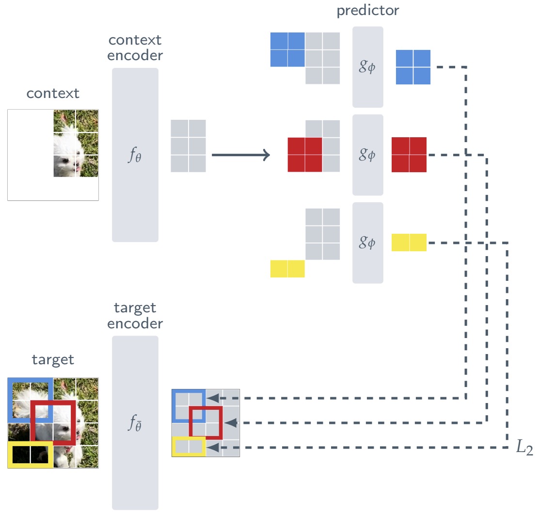
Training Dynamics
-
I-JEPA training relies on several mechanisms to ensure stability and scalability:
- EMA target encoder: provides slowly evolving targets, reducing training instability.
- No reconstruction decoder: reduces computational cost and avoids modeling irrelevant details.
- Latent prediction loss: focuses on semantic consistency.
-
Importantly, the model does not require:
- Negative samples, as in contrastive learning
- Pixel-level losses, as in generative modeling
- Strong data augmentations
-
This simplicity contributes to scalability.
I-JEPA as a State Abstraction Rather Than a Renderer
-
I-JEPA does not attempt to render missing pixels. This is its main distinction from masked autoencoders and diffusion-style visual reconstruction systems. In the renderer-simulator-planner taxonomy, reconstruction-based image models are closer to renderer models because their objective is observation fidelity. I-JEPA instead learns a compact visual state abstraction that is useful for later prediction.
-
This matters for world modeling because a simulator does not need to reproduce every sensory detail. It needs a state representation that supports stable prediction. I-JEPA supplies the image-level version of that idea: predict the latent content of missing regions, not their exact pixel realization.
Representation Properties
-
The representations learned by I-JEPA exhibit several desirable properties:
- Semantic abstraction: captures object-level and scene-level information.
- Robustness: less sensitive to low-level variations.
- Transferability: performs well across downstream tasks such as classification, detection, and depth estimation.
-
Empirically, I-JEPA achieves strong performance on ImageNet linear evaluation while requiring less compute than competing methods. Self-Supervised Learning from Images with a Joint-Embedding Predictive Architecture by Assran et al. (2023) reports strong downstream performance across classification, object counting, and depth prediction while avoiding view augmentations during pretraining.
Comparison with Masked Autoencoders
- Masked autoencoders (MAE) reconstruct pixel values:
- In contrast, I-JEPA predicts latent representations:
-
This difference has important implications:
- MAE must model high-frequency details.
- I-JEPA focuses on predictable structure.
- I-JEPA can ignore noise and stochastic variations.
-
From the functional-taxonomy perspective, MAE is more renderer-adjacent because it reconstructs observations, while I-JEPA is more simulator-adjacent because it trains a latent state representation without requiring observation-level output.
Scaling Behavior
-
I-JEPA scales effectively with model size and data. Using Vision Transformers, it can be trained efficiently on large datasets:
- Large models converge with fewer epochs.
- Performance improves with larger context and target regions.
- Training remains stable due to EMA targets.
-
The method demonstrates that latent prediction is a viable alternative to both contrastive and generative objectives at scale.
Limitations
-
Despite its advantages, I-JEPA has several limitations:
- No explicit temporal modeling: operates on single images.
- Limited interaction reasoning: patch-based masking does not enforce object-level dynamics.
- Deterministic predictions: does not explicitly model uncertainty.
-
These limitations motivate extensions to video, sequential modeling, and probabilistic formulations.
-
I-JEPA also lacks the full functional breadth of a world model. It is not a renderer because it does not generate observations, it is not a planner because it does not output actions, and it is only a partial simulator because it models static latent compatibility rather than temporal state transitions. Its importance lies in providing the representation-space prediction principle that later world-model systems extend.
Transition to Video and World Modeling
-
To become a full world model, JEPA must incorporate temporal structure and action conditioning. This leads to video-based extensions where the model predicts future latent states from past observations.
-
The next section examines V-JEPA and V-JEPA 2, which extend I-JEPA to video and enable understanding, prediction, and planning in dynamic environments.
Video JEPA and Scalable World Modeling
-
Extending JEPA from images to video transforms a static representation learner into a temporal predictive system. Video-based JEPA models learn to capture dynamics, motion, and temporal structure directly from sequences of observations, enabling the emergence of world modeling capabilities.
-
In the functional taxonomy of world models, video JEPA occupies an important middle ground. It is not a renderer-first model because it does not train by generating full video frames. It is not yet a complete planner unless actions and goals are introduced. Its core role is simulator-like: it learns latent state evolution from video, preserving the predictable structure needed for downstream understanding and control. A Functional Taxonomy of World Models separates renderers, simulators, and planners by output type, which clarifies why video generation and video latent prediction should not be treated as identical forms of world modeling.
From Spatial to Spatiotemporal Prediction
-
In I-JEPA, the prediction task is spatial: masked regions of an image are predicted from visible context. In video, this generalizes to spatiotemporal prediction:
\[\hat{s}_{t+\Delta} = g_\phi(s_{\le t}, \xi)\]- where \(\Delta\) denotes a future time offset and \(\xi\) encodes temporal position or masking structure.
-
Instead of predicting pixels across time, video JEPA predicts latent embeddings of masked spatiotemporal regions. This allows the model to focus on predictable dynamics such as motion trajectories and object interactions, rather than reconstructing full video frames.
Video Renderers versus Video Latent Simulators
-
A video renderer models what future observations should look like:
\[\hat{o}_{t+1:t+H} \sim p_\theta(o_{t+1:t+H}\mid o_{\le t},c)\]- where \(c\) may include text, camera motion, user input, or previous frames. This paradigm is useful for visual creation and imagination, but it can optimize visual plausibility without enforcing physically valid state transitions.
-
A video latent simulator models how the underlying representation evolves:
- This distinction matters because video generation can produce plausible images while failing to preserve object identity, geometry, contact, or causal consistency. Video JEPA is explicitly closer to the simulator side because it learns latent dynamics rather than frame synthesis. V-JEPA 2: Self-Supervised Video Models Enable Understanding, Prediction and Planning by Assran et al. (2025) frames this distinction directly by using representation-space prediction instead of video generation for scalable world modeling.
V-JEPA: Learning Dynamics from Video
-
Video JEPA models operate by masking portions of video clips and predicting their latent representations. The key design principles remain consistent:
- Prediction in latent space
- Masking-based task construction
- Separation of context and target encoders
-
However, temporal structure introduces new challenges:
- Capturing motion and temporal dependencies
- Maintaining consistency across frames
- Avoiding trivial interpolation solutions
-
These are addressed through structured masking and temporal encoding.
V-JEPA 2: Scaling to Internet Video
-
V-JEPA 2: Self-Supervised Video Models Enable Understanding, Prediction and Planning by Assran et al. (2025) demonstrates that JEPA can scale to internet-scale video and serve as a foundation for world modeling. The paper reports pretraining on a video and image dataset comprising more than one million hours of internet video, followed by action-conditioned post-training on a smaller amount of robot interaction data.
-
The model is trained using a mask-denoising latent prediction objective. Unlike generative video models, it does not attempt to synthesize frames. Instead, it learns representations that capture:
- Motion dynamics
- Object behavior
- Temporal dependencies
- Appearance and action-relevant structure
Representation Learning at Scale
-
The scale of training data fundamentally changes the capabilities of the learned representation. V-JEPA 2 demonstrates that large-scale self-supervised video training yields representations that support:
- Action recognition: identifying activities from video
- Action anticipation: predicting future actions
- Video question answering: reasoning about temporal events
-
These capabilities emerge without explicit supervision for these tasks during the core self-supervised pretraining stage, indicating that the model captures high-level semantic and temporal structure. V-JEPA 2 by Assran et al. (2025) reports strong motion understanding, state-of-the-art human action anticipation, and video question-answering performance after language alignment.
Action-Free Pretraining
- A key insight is that meaningful world models can be learned without action labels. Video provides sequences of states:
- From these, the model learns implicit dynamics:
-
This enables large-scale pretraining using passive data, which is far more abundant than interaction data.
-
In the functional taxonomy, this is the transition from observation sequences to a simulator-like latent model. The model does not yet know which actions caused the observed transitions, but it learns regularities of motion, persistence, occlusion, and temporal change that later action-conditioned models can exploit. A Functional Taxonomy of World Models emphasizes that simulation is the bridge between rendering and planning because it captures how the world changes, not merely how it appears.
Action-Conditioned Post-Training
- To enable control and planning, V-JEPA 2 introduces a second stage where actions are incorporated:
-
This stage uses a relatively small amount of robot interaction data to learn action-conditioned dynamics on top of the pretrained representation. V-JEPA 2 by Assran et al. (2025) reports post-training an action-conditioned world model, V-JEPA 2-AC, using less than 62 hours of unlabeled robot videos from the DROID dataset.
-
The resulting model, V-JEPA 2-AC, supports planning by simulating trajectories in latent space.
Planning in Latent Space
- Planning is performed using model predictive control (MPC) in the learned latent space. Given a goal state \(z^*\), the system searches for an action sequence that minimizes a cost function:
-
The latent dynamics model is used to simulate candidate trajectories efficiently.
-
This approach avoids the computational cost of generating full video frames during planning. Functionally, it converts a simulator-style latent world model into a planner substrate: the model predicts possible futures, and the control loop selects the action sequence whose predicted future best matches the goal.
Relation to 3D and Spatial World Generation
-
Video JEPA learns from temporal observation sequences, while emerging spatial world models try to construct editable 3D environments. The two approaches address related but distinct problems. Video JEPA emphasizes latent temporal prediction, whereas 3D world generation emphasizes spatial state construction, view consistency, and editability.
-
Marble: A Multimodal World Model describes a system that creates editable 3D worlds from text, images, video, or coarse 3D layouts and can export worlds as Gaussian splats, meshes, or videos, placing it closer to the simulator-renderer boundary. A Functional Taxonomy of World Models situates this kind of work within a broader spatial-intelligence agenda, where world models must ultimately support rendering, simulation, and planning.
Advantages over Generative Video Models
-
Compared to generative video models, JEPA-based video models offer several advantages:
- Efficiency: no need to generate high-resolution frames
- Focus: emphasizes predictable dynamics rather than visual detail
- Scalability: leverages large-scale video data effectively
- Planning compatibility: directly produces latent states for control
-
Generative models often prioritize visual fidelity, while JEPA prioritizes predictive utility. In the functional taxonomy, this is the distinction between renderer optimization and simulator optimization: renderers must look right, while simulators must support reliable state evolution.
Limitations and Challenges
-
Despite its strengths, video JEPA faces several challenges:
- Implicit action inference: action-free pretraining does not explicitly model causality
- Deterministic predictions: uncertainty is not always captured
- Limited object structure: patch-based representations may miss object-level interactions
-
These limitations motivate extensions that incorporate:
- Action conditioning during training
- Object-centric representations
- Probabilistic modeling of uncertainty
- Explicit 3D or spatial state structure
-
Video JEPA also inherits a broader challenge from the simulator paradigm: a compact latent state may support prediction while remaining difficult to inspect, edit, or validate. This matters when world models are used in safety-critical robotics, driving, or scientific settings.
Transition to Advanced JEPA World Models
-
The progression from I-JEPA to V-JEPA 2 demonstrates how predictive representation learning scales from static perception to dynamic world understanding and planning.
-
The next section explores advanced JEPA-based world models, including object-centric, causal, sequential, and probabilistic variants that address the limitations of current approaches.
Advanced JEPA World Models
-
While I-JEPA and V-JEPA establish the core paradigm of latent predictive learning, they do not fully address key requirements for robust world modeling: interaction reasoning, uncertainty, temporal abstraction, object permanence, and structured representations. Recent work extends JEPA along multiple axes to address these limitations, resulting in a family of advanced world models.
-
In the renderer-simulator-planner taxonomy, these advanced variants primarily strengthen the simulator and planner roles. They make latent state more sequential, object-centric, causal, probabilistic, or action-conditioned, which moves JEPA closer to the requirements of embodied intelligence. A Functional Taxonomy of World Models emphasizes that world models should be evaluated by function: rendering observations, simulating state, or planning actions.
Sequential JEPA and Temporal Structure
-
Standard JEPA formulations predict targets independently, without modeling sequential dependencies between predictions. However, real-world perception is inherently sequential and structured.
-
seq-JEPA: Autoregressive Predictive Learning of Invariant-Equivariant World Models by Ghaemi et al. (2026) introduces a sequential formulation that processes a series of observations and actions:
-
The model learns two types of representations:
- Equivariant representations at the level of individual observations
- Invariant representations at the level of aggregated sequence embeddings
-
This architectural separation resolves the trade-off between capturing fine-grained transformations and supporting high-level tasks such as classification.
-
DSeq-JEPA: Discriminative Sequential Joint-Embedding Predictive Architecture by He et al. (2026) further introduces ordered prediction, where targets are predicted sequentially based on importance:
-
This imposes a curriculum over prediction tasks, improving representation quality and interpretability.
-
From the functional-taxonomy perspective, sequential JEPA strengthens the simulator role because it learns how latent state evolves across ordered observations, not merely how isolated views relate.
Object-Centric and Causal JEPA
-
Patch-based masking does not enforce reasoning about interactions between entities. To address this, object-centric JEPA variants operate on structured representations.
-
Causal-JEPA: Learning World Models through Object-Level Latent Interventions by Nam et al. (2026) introduces object-level masking:
- During training, subsets of object representations are masked, and the model must infer them from other objects:
-
This induces a causal inductive bias, as the model must reason about interactions rather than relying on local correlations.
-
The following figure (source) shows the C-JEPA training pipeline, where object-level masking forces inference of masked object states from surrounding context. Specifically, it shows how object-centric masking induces interaction reasoning and causal structure in latent space. A frozen encoder extracts object-centric representations, followed by selective masking across history. The predictor recovers masked history slots and predicts future latent states, conditioned on optional auxiliary variables, via a joint masked-history and forward-prediction objective.
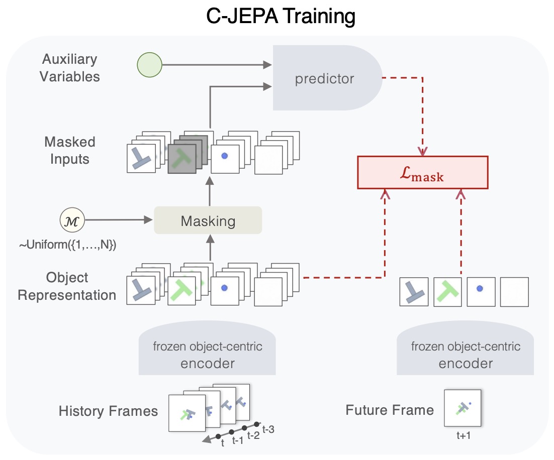
-
This approach significantly improves performance on tasks requiring counterfactual reasoning and planning.
-
Object-centric JEPA is especially aligned with simulator-style world modeling. A useful simulator should not only predict latent feature vectors; it should expose stable entities, relations, and interventions. Object-level latent masking pushes the representation toward this form by making interaction structure necessary for prediction.
Spatial and 3D World Models
-
The functional taxonomy highlights that world modeling is not only temporal but also spatial. A model may need to represent a scene as a navigable, editable, physically meaningful 3D structure rather than as a sequence of 2D frames. This motivates spatial world models that combine aspects of renderers and simulators.
-
Marble: A Multimodal World Model describes a system that generates editable 3D worlds from text, images, video, or layout inputs and exports them as Gaussian splats, meshes, or videos. This kind of model is renderer-like when it produces views, but simulator-like when it maintains editable scene structure.
-
For JEPA, spatial world modeling suggests an important direction: predict structured latent scene state rather than patch embeddings alone. A future 3D-JEPA-style system could predict object pose, geometry, affordances, and interaction-relevant latent fields without reconstructing every pixel.
Multimodal and Motion-Aware JEPA
-
Real-world environments involve multiple modalities and dynamic processes. Extensions of JEPA incorporate additional signals:
-
MC-JEPA: A Joint-Embedding Predictive Architecture for Self-Supervised Learning of Motion and Content Features by Bardes et al. (2023) jointly learns semantic content and motion via optical flow estimation:
-
This enables representations that capture both appearance and dynamics.
-
A-JEPA: Joint-Embedding Predictive Architecture Can Listen by Fei et al. (2023) extends JEPA to audio, using time-frequency masking strategies to capture temporal structure in spectrograms.
-
These models demonstrate that JEPA is a general predictive learning framework across modalities.
-
From a functional perspective, multimodal JEPA expands the observation interface of a world model. A robust agent should be able to map audio, vision, proprioception, language, and action histories into a shared predictive state.
Probabilistic JEPA and Uncertainty Modeling
-
Deterministic JEPA models predict a single latent embedding, which limits their ability to represent uncertainty.
-
Variational JEPA: Probabilistic World Models by Huang (2026) introduces a probabilistic formulation:
- with a variational objective:
-
This enables:
- Uncertainty estimation via sampling
- Robust prediction in stochastic environments
- Planning under uncertainty
-
The framework connects JEPA to predictive state representations and Bayesian filtering.
-
Probabilistic JEPA is important for simulator and planner world models because a single predicted future is often insufficient. A planner must reason over multiple possible futures when observations are partial, dynamics are stochastic, or other agents behave unpredictably.
End-to-End JEPA World Models
-
Many JEPA systems rely on pre-trained encoders or asymmetric mechanisms such as stop-gradient and EMA target networks to prevent collapse. End-to-end approaches instead combine latent prediction with explicit regularization so that the encoder and predictor can be optimized jointly.
-
LeWorldModel: Stable End-to-End Joint-Embedding Predictive Architecture from Pixels by Maes et al. (2026) proposes a minimal formulation:
\[\mathcal{L} = \left\| \hat{z}_{t+1}-z_{t+1} \right\|_2^2 + \lambda \mathcal{L}_{\mathrm{SIGReg}}\]- where the first term learns action-conditioned temporal dynamics and SIGReg prevents representational collapse by encouraging the latent distribution to match an isotropic Gaussian.
-
The following figure (source) shows the LeWorldModel training pipeline, where observations are encoded into latent states and the predictor autoregressively predicts the next latent state conditioned on the current state and action. The encoder and predictor are jointly optimized without stop-gradient, EMA target networks, or pretrained representations, while SIGReg regularizes the learned latent space.
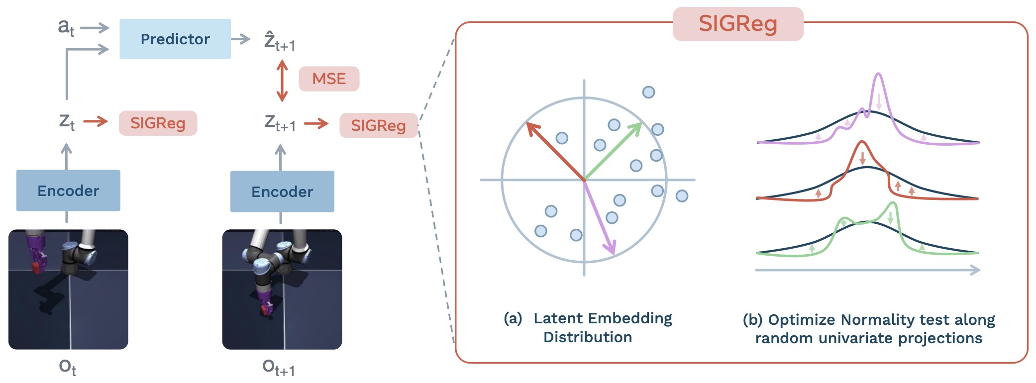
-
LeWorldModel inherits this distribution-matching principle from LeJEPA: Provable and Scalable Self-Supervised Learning Without the Heuristics by Balestriero and LeCun (2025), which introduces SIGReg as an alternative to heuristic anti-collapse mechanisms. SIGReg projects embeddings onto randomly sampled one-dimensional directions and applies a Gaussian goodness-of-fit objective to the projected distributions; aggregating these constraints encourages the full representation distribution toward an isotropic Gaussian.
-
LeWorldModel extends this idea from multi-view representation learning to action-conditioned temporal dynamics. Instead of using a frozen or slowly updated target representation, gradients can flow jointly through the encoder and dynamics predictor, while SIGReg prevents the latent prediction objective from converging to complete or dimensional collapse. This provides a simple end-to-end route from pixels to compact predictive states suitable for simulation and control.
Unified World Models
-
A fully general world model would combine the three functional roles:
- Renderer: generate observations from state.
- Simulator: roll forward latent or explicit world state.
- Planner: choose actions that achieve goals.
-
The following figure (source) shows the convergence toward unified world models that combine rendering, simulation, and planning. Specifically, it shows a unified world-model architecture in which rendering produces interpretable observations, simulation maintains and evolves world state, and planning selects actions by evaluating predicted futures.
- Advanced JEPA systems mostly strengthen the simulator and planner components, but they could be combined with renderers when human-interpretable visual output is needed. For example, a JEPA latent simulator could provide compact predictive dynamics, while a renderer decodes selected latent states into observations for inspection or communication.
Unifying Perspective
-
These extensions collectively transform JEPA into a comprehensive world modeling framework:
- Sequential JEPA captures temporal dependencies
- Object-centric JEPA models interactions and causality
- Spatial world models expose editable 3D scene structure
- Multimodal JEPA integrates diverse sensory inputs
- Probabilistic JEPA represents uncertainty
- End-to-end JEPA simplifies training and improves scalability
-
Together, they address the core challenges of world modeling: representation, dynamics, interaction, uncertainty, and action selection.
Transition to Implementation
-
While the conceptual framework of JEPA is well-defined, practical deployment requires careful design choices in architecture, masking, optimization, and scaling.
-
The next section provides detailed implementation guidance, including architectural configurations, training procedures, and engineering considerations for building JEPA-based world models.
Implementation Details for JEPA-Based World Models
-
Building a JEPA-based world model requires choosing the representation format, prediction target, masking policy, predictor architecture, collapse-prevention strategy, and planning interface. The implementation should be designed around the intended domain: images, video, audio, robotics, object-centric environments, or spatial 3D worlds.
-
The renderer-simulator-planner taxonomy is useful at implementation time because it forces the central design question: what should the system output? A renderer needs an observation decoder, a simulator needs a reliable latent or explicit state transition model, and a planner needs an action-selection mechanism. A Functional Taxonomy of World Models frames this distinction by separating world models according to whether they produce observations, states, or actions.
Data Representation
- For image and video models, observations are usually converted into patch or tubelet tokens:
- For video, tubelets preserve local spatiotemporal structure:
- For object-centric models, a frozen or trainable object encoder maps observations into object slots:
-
This object-level representation is useful when the task depends on interaction, counterfactual reasoning, or physical causality, as in Causal-JEPA: Learning World Models through Object-Level Latent Interventions by Nam et al. (2026).
-
For spatial world models, the representation may instead be a 3D scene state, such as a mesh, point cloud, radiance field, Gaussian splat field, voxel grid, scene graph, object layout, or hybrid latent field. Marble: A Multimodal World Model illustrates this design space by producing editable 3D worlds from text, image, video, or coarse 3D layout inputs and exporting them in multiple visual or geometric formats.
Renderer, Simulator, and Planner Interfaces
-
A JEPA-based system should expose different interfaces depending on its intended role.
-
A renderer interface maps latent state to observations:
-
This decoder is optional in JEPA and is often omitted when the objective is representation learning or planning efficiency.
-
A simulator interface maps current latent state and action to future latent state:
-
This is the natural interface for JEPA world models, because the model is trained to predict representations rather than pixels.
-
A planner interface maps current state and goal to actions:
-
or searches over candidate action sequences:
\[a_{t:t+H}^* =\arg\min_{a_{t:t+H}} \sum_{k=1}^{H} d(\hat{z}_{t+k},z_g)\] -
This separation makes the implementation modular: a latent JEPA simulator can be paired with a renderer for visualization, a planner for control, or both.
Encoder Design
-
Most JEPA implementations use Transformer encoders. A standard image configuration follows the Vision Transformer pipeline:
\[x_i = E p_i + e_i\]- where \(E\) is a patch embedding matrix and \(e_i\) is a positional embedding.
-
For video, positional information must encode both space and time:
-
Implementation choices typically include:
- Patch size: smaller patches improve detail but increase compute.
- Embedding dimension: larger dimensions improve capacity but increase memory.
- Depth: deeper encoders improve abstraction.
- Attention windowing: local attention can reduce video compute.
-
I-JEPA by Assran et al. (2023) uses Vision Transformers and shows that scaling the encoder improves representation quality while avoiding pixel reconstruction.
-
For spatial models, encoder design may require fusing 2D and 3D information. A practical architecture may use an image encoder for appearance, a depth or geometry encoder for spatial structure, and a cross-attention module to bind them into a scene-level latent state. This is especially relevant when the system is expected to simulate editable environments rather than only predict future video embeddings.
Target Encoder
-
The target encoder provides embeddings for masked or future targets. In many JEPA systems, it is an exponential moving average of the context encoder:
\[\bar{\theta} \leftarrow m \bar{\theta} + (1-m)\theta\]- where \(m\) is the EMA momentum.
-
A high momentum value makes target representations stable, reducing oscillation and helping avoid collapse. The target encoder is usually used with stop-gradient:
\[s_y = \text{sg}(f_{\bar{\theta}}(y))\]- where \(\text{sg}(\cdot)\) prevents gradients from flowing into the target branch.
-
An EMA target encoder is a common stabilization mechanism rather than a fundamental requirement of JEPA. An alternative is to regularize the latent distribution directly so that the prediction objective cannot exploit collapsed solutions. VICReg: Variance-Invariance-Covariance Regularization for Self-Supervised Learning by Bardes et al. (2022) demonstrates that explicit variance and covariance regularization can stabilize joint-embedding learning without requiring an asymmetric teacher-student architecture, while LeJEPA: Provable and Scalable Self-Supervised Learning Without the Heuristics by Balestriero and LeCun (2025) goes further by using SIGReg to enforce an isotropic Gaussian embedding distribution without stop-gradient or a teacher-student EMA network.
Predictor Architecture
-
The predictor maps context embeddings to target embeddings:
\[\hat{s}_y = g_\phi(s_x, q_y)\]- where \(q_y\) is a query embedding that encodes the target position, time, object identity, or action.
-
A common implementation is a lightweight Transformer decoder or MLP-Transformer hybrid:
-
For action-conditioned world models, the predictor conditions on actions:
\[\hat{z}_{t+1} = g_\phi(z_t, a_t)\]-
or over a horizon:
\[\hat{z}_{t+k+1} = g_\phi(\hat{z}_{t+k}, a_{t+k})\]
-
-
V-JEPA 2: Self-Supervised Video Models Enable Understanding, Prediction and Planning by Assran et al. (2025) uses action-conditioned post-training to adapt video representations for robot planning.
-
For planner-oriented systems, the predictor must be stable under rollout. One-step prediction quality is not sufficient; errors compound across imagined trajectories. In practice, this motivates scheduled rollout training, latent consistency losses, short-horizon regularization, or model predictive control with frequent replanning.
Masking Policies
-
Masking determines what the model must predict. Poor masking can make the task too easy or too hard.
-
For images, useful masking policies include:
- Large target blocks: encourage semantic prediction.
- Distributed context blocks: preserve enough global information.
- Multiple targets per image: improve coverage.
-
For video, masking should cover spatiotemporal regions:
-
Good video masks force the model to infer motion rather than interpolate nearby frames.
-
For audio, masking must respect time-frequency correlations. A-JEPA: Joint-Embedding Predictive Architecture Can Listen by Fei et al. (2023) uses curriculum masking that gradually shifts from random block masking to time-frequency-aware masking.
-
For object-centric models, object-level masking can enforce relational reasoning:
-
This prevents the model from relying only on local patch continuity.
-
For spatial world models, masking can operate over camera views, 3D regions, object slots, depth layers, or scene graph nodes. A simulator-oriented mask should remove enough structure to require spatial reasoning, while still preserving enough context to make the target predictable.
Loss Functions
- The base JEPA loss is a latent regression loss:
- For multi-task JEPA systems, additional terms may be added:
-
For motion-aware JEPA, MC-JEPA: A Joint-Embedding Predictive Architecture for Self-Supervised Learning of Motion and Content Features by Bardes et al. (2023) combines latent prediction with optical-flow supervision or self-supervised flow estimation.
-
For end-to-end pixel-based world models, LeWorldModel: Stable End-to-End Joint-Embedding Predictive Architecture from Pixels by Maes et al. (2026) combines next-embedding prediction with SIGReg, a random-projection distributional regularizer derived from LeJEPA: Provable and Scalable Self-Supervised Learning Without the Heuristics by Balestriero and LeCun (2025), to encourage latent embeddings to follow an isotropic Gaussian distribution and prevent collapse without a stop-gradient or EMA target encoder.
-
For renderer-simulator hybrids, an optional observation reconstruction or rendering loss may be added:
- but this should be used carefully. If it dominates the objective, the system can drift back toward modeling high-entropy visual details rather than compact predictive state.
Collapse Prevention
- Collapse occurs when the encoder maps all inputs to the same representation:
-
This can minimize latent prediction loss while producing useless representations.
-
Common anti-collapse mechanisms include:
- EMA target encoders
- Stop-gradient target branches
- Predictor bottlenecks
- Variance or covariance regularization
- Distributional regularizers
- Careful masking
-
A simple diagnostic is the per-dimension feature variance:
- If many dimensions have near-zero variance, the representation is collapsing.
Collapse Prevention: VICReg and SIGReg
-
A latent prediction objective alone does not rule out degenerate solutions. If every observation is mapped to the same constant representation \(f_\theta(o)=c\), then a predictor can trivially reproduce the target representation while the latent state contains no useful information about the observation. More generally, collapse can be complete, where all samples map to nearly the same point, or dimensional, where embeddings occupy only a low-dimensional subspace. VICReg: Variance-Invariance-Covariance Regularization for Self-Supervised Learning by Bardes et al. (2022) makes collapse prevention explicit through variance and covariance constraints, while LeJEPA: Provable and Scalable Self-Supervised Learning Without the Heuristics by Balestriero and LeCun (2025) reframes the problem as matching the entire embedding distribution to an isotropic Gaussian.
-
These approaches are useful for understanding two progressively stronger notions of a well-behaved latent space. VICReg constrains low-order statistics: individual dimensions should have sufficient variance and different dimensions should be decorrelated. SIGReg instead asks whether the multivariate embedding distribution itself matches a prescribed target distribution. The distinction is important because matching a finite set of moments does not, in general, uniquely identify a distribution. LeJEPA by Balestriero and LeCun (2025) uses this observation to motivate distribution-level rather than moment-level regularization.
VICReg: Variance-Invariance-Covariance Regularization
-
VICReg: Variance-Invariance-Covariance Regularization for Self-Supervised Learning by Bardes et al. (2022) introduces a non-contrastive joint-embedding objective that explicitly separates representation learning into three requirements: corresponding views should be invariant, every embedding dimension should retain non-zero variance, and different dimensions should carry non-redundant information. Unlike contrastive objectives, VICReg does not require negative samples or memory banks; unlike asymmetric self-distillation methods, collapse prevention does not intrinsically require a stop-gradient branch, momentum encoder, or shared parameters between the two branches.
-
Given two transformations of the same input \(x=t(i), \qquad x'=t'(i)\), two encoder-expander branches produce batches of embeddings
\[Z=[z_1,\ldots,z_N], \qquad Z'=[z'_1,\ldots,z'_N],\]- with each embedding in \(\mathbb{R}^D\). In the standard implementation, the encoder representation is intended for downstream use, while an expander maps it into the higher-dimensional space in which VICReg is optimized. VICReg by Bardes et al. (2022) uses a ResNet-50 encoder with a three-layer, 8192-dimensional expander in its principal ImageNet configuration and discards the expander after pretraining.
-
The following figure (source) shows the VICReg joint-embedding architecture: two transformed views are encoded and expanded into embeddings, corresponding embeddings are pulled together through an invariance loss, per-coordinate variance is kept above a threshold, and off-diagonal covariance is suppressed to reduce redundancy.
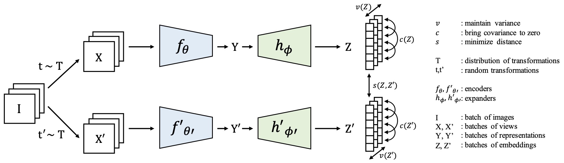
-
The invariance term minimizes the mean squared distance between embeddings of corresponding views:
\[s(Z,Z') = \frac{1}{N} \sum_{i=1}^{N} \left\| z_i-z'_i \right\|_2^2\]- By itself, however, this objective admits the constant solution \(z_i=z'_i=c\) for every sample. VICReg therefore regularizes each branch independently rather than relying on invariance alone. VICReg by Bardes et al. (2022) shows experimentally that the invariance-only objective collapses without an additional mechanism that preserves feature dispersion.
-
The variance term prevents complete collapse by requiring every coordinate to maintain a minimum batch standard deviation. For coordinate \(j\),
\[S(z^{(j)},\epsilon) = \sqrt{ \operatorname{Var}(z^{(j)})+\epsilon }\]- and:
- Here, \(\gamma\) is the desired minimum standard deviation and \(\epsilon\) prevents numerical instability. The standard configuration uses \(\gamma=1\) and \(\epsilon=10^{-4}\). The hinge form is important: dimensions already exhibiting sufficient spread are not continually pushed toward increasing variance, whereas dimensions approaching collapse receive a repulsive gradient. VICReg by Bardes et al. (2022) specifically applies the penalty to standard deviation rather than variance because the variance gradient itself becomes small near a collapsed solution.
-
Variance alone does not guarantee a rich \(D\)-dimensional representation. Multiple coordinates could remain non-constant while carrying nearly identical information. VICReg therefore computes the within-branch covariance matrix:
\[C(Z) = \frac{1}{N-1}\sum_{i=1}^{N}(z_i-\bar{z})(z_i-\bar{z})^\top\]-
where:
\[\bar{z} = \frac{1}{N} \sum_{i=1}^{N}z_i,\]-
and penalizes its off-diagonal entries:
\[c(Z) = \frac{1}{D} \sum_{i\neq j} C(Z)_{ij}^{2}\]
-
-
This covariance term encourages different coordinates to encode complementary information rather than co-varying redundantly. It is closely related to the redundancy-reduction principle of Barlow Twins: Self-Supervised Learning via Redundancy Reduction by Zbontar et al. (2021), but VICReg applies covariance regularization independently within each branch and uses explicit variance preservation instead of relying on standardized cross-correlations.
-
-
The complete VICReg objective is therefore
\[\mathcal{L}_{\mathrm{VICReg}} = \lambda s(Z,Z') + \mu \left[ v(Z)+v(Z') \right] + \nu \left[ c(Z)+c(Z') \right]\]- where \(\lambda\) controls invariance, \(\mu\) controls variance preservation, and \(\nu\) controls covariance reduction. The principal ImageNet configuration in VICReg by Bardes et al. (2022) uses \(\lambda=\mu=25\) and \(\nu=1\).
-
Conceptually, VICReg separates two kinds of degeneracy. The variance term prevents all samples from shrinking toward the same embedding, while the covariance term prevents a representation with nominally active but highly redundant dimensions. Ablations in VICReg by Bardes et al. (2022) show that invariance alone and invariance plus covariance collapse, whereas adding variance prevents the constant solution; covariance then improves the information distribution across dimensions.
-
This formulation is especially relevant to multimodal and world-model settings because the regularizers act on each branch independently. The two branches need not share parameters, architecture, or even input modality. VICReg by Bardes et al. (2022) demonstrates this property with image-text and video-audio settings, making the formulation applicable when compatible observations are structurally different rather than merely augmented copies of the same image.
SIGReg: From Moment Regularization to Distribution Matching
-
VICReg constrains low-order geometry: each coordinate must retain sufficient spread and off-diagonal covariance is suppressed, while invariance aligns corresponding views. These conditions are effective against collapse, but they do not uniquely determine the shape of the embedding distribution. A representation can have non-degenerate coordinates and identity covariance while remaining concentrated on a highly structured, non-Gaussian subset of the space. LeJEPA: Provable and Scalable Self-Supervised Learning Without the Heuristics by Balestriero and LeCun (2025) uses this limitation of finite-moment constraints to motivate distribution-level regularization.
-
This matters particularly in general-purpose self-supervised pretraining, where the downstream task is not known in advance and the frozen representation may later be consumed by a linear probe, nearest-neighbor method, or other predictor. The geometry selected during pretraining therefore determines which directions retain usable variation. A representation that becomes thin or degenerate along some directions can deprive an unknown downstream predictor of information even when simple variance and covariance diagnostics appear acceptable.
-
LeJEPA by Balestriero and LeCun (2025) therefore proposes a stronger target: an isotropic Gaussian embedding distribution. Under the task-family and estimator assumptions developed in the paper, this distribution minimizes worst-case downstream prediction risk, providing a minimax rationale for avoiding privileged or information-poor directions when the future task is unknown:
\[Z \sim \mathcal{N}(0,I_D)\] -
Geometrically, this target corresponds to a directionally balanced latent cloud rather than one concentrated along a small number of axes or manifolds. The isotropic Gaussian does not privilege a particular direction, so every unit direction has the same projected variance. SIGReg turns this geometric desideratum into a tractable training objective.
-
Directly testing whether a high-dimensional minibatch forms this isotropic Gaussian is difficult. SIGReg therefore tests one-dimensional random projections, analogous to observing many shadows of the same high-dimensional point cloud. For a unit vector \(a\in\mathbb{S}^{D-1},\) an embedding \(z\) is projected to the scalar \(u=a^\top z\). If \(Z\sim\mathcal{N}(0,I_D),\) every unit-norm projection satisfies \(a^\top Z\sim\mathcal{N}(0,1)\). Conversely, the Cramér-Wold principle implies that equality of all one-dimensional projections identifies the multivariate distribution. LeJEPA by Balestriero and LeCun (2025) exploits this property to replace a difficult multivariate test with many inexpensive univariate Gaussian goodness-of-fit tests.
-
For a minibatch of embeddings \(\{z_n\}_{n=1}^{N}\), and a set of random directions \(\mathcal{A} = \{a_1,\ldots,a_M\}\), SIGReg applies a univariate statistic \(T\) to each projected sample set and averages the resulting penalties:
\[\operatorname{SIGReg}_{T} \left( \mathcal{A}, \{z_n\}_{n=1}^{N} \right) = \frac{1}{|\mathcal{A}|} \sum_{a\in\mathcal{A}} T \left( \{a^\top z_n\}_{n=1}^{N} \right)\]- The averaging operation is used during optimization rather than selecting only the worst projection, because it distributes gradients across the sampled directions. LeJEPA by Balestriero and LeCun (2025) recommends a characteristic-function-based Epps-Pulley statistic for \(T\) because it provides stable bounded derivatives while remaining efficient for minibatch optimization.
-
The following figure (source) shows SIGReg as a projected distribution-matching procedure: an encoder maps arbitrary input data into a latent distribution, random one-dimensional projections expose slices of that distribution, and a goodness-of-fit objective pushes each projected density toward the corresponding projection of the isotropic Gaussian target.
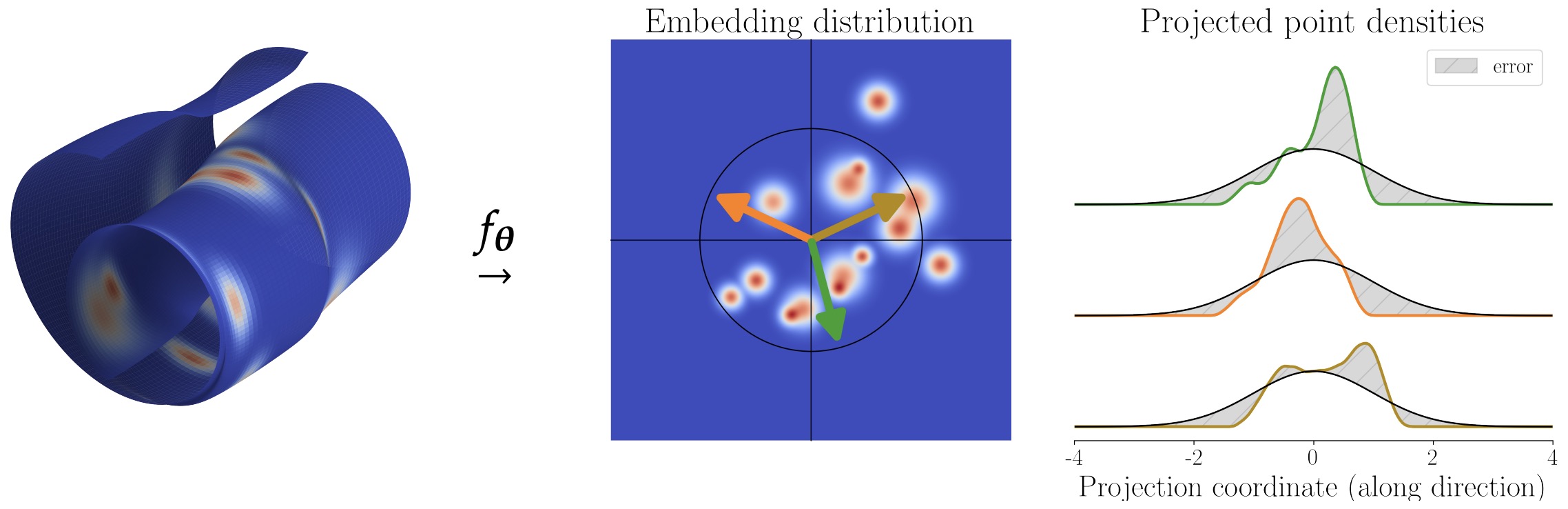
-
The use of characteristic functions addresses a limitation of simple finite-moment matching. A characteristic function \(\varphi_Z(t) = \mathbb{E}\left[e^{itZ} \right]\) uniquely determines the distribution of a random variable.
-
For a standard Gaussian, \(\varphi_{\mathcal{N}(0,1)}(t) = e^{-t^2/2}\). A characteristic-function goodness-of-fit statistic can therefore compare empirical projected embeddings against the Gaussian target across a continuum of frequencies rather than checking only a fixed set of moments. LeJEPA by Balestriero and LeCun (2025) selects the Epps-Pulley family after comparing moment-based, cumulative-distribution-based, and characteristic-function-based tests.
-
This distinction is visible in the X-shaped construction analyzed in LeJEPA by Balestriero and LeCun (2025). Its coordinate marginals can be standard Gaussian and its covariance can be the identity even though probability mass remains concentrated along two crossing structures rather than filling the plane like a Gaussian. Coordinate-wise variance and covariance therefore do not reveal the higher-order degeneracy. Projections along suitable directions do: their one-dimensional distributions depart from Gaussianity and receive a large goodness-of-fit penalty.
-
The following figure (source) shows an X-shaped non-Gaussian distribution with standard-Gaussian marginals and identity covariance, together with multiple one-dimensional projections; although low-order marginal statistics appear valid, appropriately oriented projections reveal the joint degeneracy through large goodness-of-fit statistics.
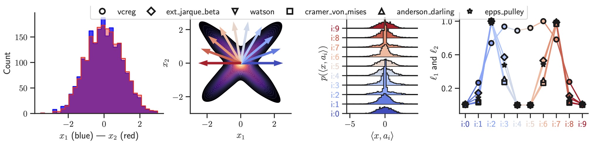
- Projection directions are resampled during training rather than permanently fixing a small set of slices. Each minibatch therefore probes a new collection of directions, progressively covering the hypersphere while avoiding the cost of an explicit high-dimensional density test. LeJEPA by Balestriero and LeCun (2025) implements this sketching strategy with the Epps-Pulley statistic and retains linear time and memory complexity in minibatch size.
LeJEPA: Prediction Plus SIGReg
-
SIGReg becomes a JEPA objective when combined with a predictive agreement term. For embeddings \(z_{n,v}\) from multiple compatible views, LeJEPA by Balestriero and LeCun (2025) uses a squared-distance prediction objective together with SIGReg on each view:
\[\mathcal{L}_{\mathrm{LeJEPA}} = \lambda \frac{1}{V} \sum_{v=1}^{V} \operatorname{SIGReg} \left( \{z_{n,v}\}_{n=1}^{B} \right) + (1-\lambda) \frac{1}{B} \sum_{n=1}^{B} \mathcal{L}_{\mathrm{pred}} \left( \{z_{n,v}\}_{v=1}^{V} \right)\]- The prediction term makes semantically related views agree, while SIGReg prevents that agreement from being achieved through a degenerate latent space. The formulation leaves a single principal trade-off parameter \(\lambda\) between prediction and distribution regularization.
-
This differs architecturally from the EMA-based JEPA recipe. I-JEPA and V-JEPA stabilize targets using a non-gradient-updated target branch whose parameters track the context encoder through exponential moving averages. LeJEPA instead regularizes the embedding distribution directly and therefore does not require stop-gradient or a teacher-student EMA mechanism for collapse prevention. LeJEPA by Balestriero and LeCun (2025) reports stable training across ResNets, ConvNets, and Vision Transformers and across more than 60 architecture configurations using this formulation.
VICReg and SIGReg as Complementary Geometric Constraints
-
VICReg and SIGReg address the same collapse problem at different statistical levels. VICReg explicitly preserves per-coordinate dispersion and suppresses second-order redundancy, while SIGReg tests whether random one-dimensional projections match the full standard-Gaussian target. The latter can therefore detect higher-order structure that is invisible to covariance alone.
-
The distinction can be summarized as:
\[\text{VICReg: preserve variance and reduce covariance}\] \[\text{SIGReg: } Z \sim \mathcal{N}(0,I_D)\] -
These objectives should not be interpreted as one being a literal special case of the other. VICReg uses a variance hinge and an off-diagonal covariance penalty rather than enforcing exact zero mean and unit covariance, whereas SIGReg specifies a complete target distribution through projected goodness-of-fit tests. The conceptual progression is from controlling selected low-order statistics to constraining the geometry of the full embedding distribution.
Practical Choice of Collapse-Prevention Mechanism
-
The anti-collapse mechanism should therefore be treated as an architectural choice rather than an incidental training detail:
- EMA target encoder: maintains slowly evolving prediction targets and is the established recipe in I-JEPA and V-JEPA-style systems.
- VICReg: explicitly maintains feature dispersion and reduces second-order redundancy without requiring negatives, a memory bank, or an asymmetric teacher-student architecture.
- SIGReg: replaces low-order moment constraints with random-projection distribution matching toward an isotropic Gaussian and can remove the need for an EMA teacher or stop-gradient mechanism in the LeJEPA formulation.
-
For a JEPA-based world model, SIGReg is particularly attractive when the encoder and dynamics predictor are to be optimized end-to-end. Instead of maintaining a separate target network \(\bar{\theta} \leftarrow m\bar{\theta}+(1-m)\theta\), the encoder can receive gradients from both latent prediction and distribution regularization. This pattern is also used by LeWorldModel: Stable End-to-End Joint-Embedding Predictive Architecture from Pixels by Maes et al. (2026), which combines next-latent prediction with SIGReg-style Gaussian regularization to train latent dynamics directly from pixels without a pretrained representation, stop-gradient, or EMA target network.
-
Regardless of the mechanism, collapse should be monitored directly during training. Useful diagnostics include per-coordinate variance \(\operatorname{Var}(z_j) = \frac{1}{B}\sum_{i=1}^{B}(z_{ij}-\mu_j)^2\), covariance spectra, effective rank, singular-value spectra, and, for SIGReg-based models, the Gaussian goodness-of-fit statistic itself. Low coordinate variance diagnoses complete or partial feature collapse, while a highly concentrated covariance spectrum reveals dimensional collapse even when the aggregate embedding norm remains non-zero.
Training Loop
-
A typical EMA-target JEPA training step, as used by I-JEPA-style architectures, is:
- Sample observations or clips and generate context and target masks.
- Encode the context with the context encoder and targets with the stop-gradient target encoder.
- Predict target embeddings from context embeddings and minimize the latent prediction loss.
- Backpropagate through the context encoder and predictor, then update the target encoder using EMA.
-
In pseudocode:
context = apply_context_mask(batch, context_mask)
targets = apply_target_mask(batch, target_masks)

z_context = context_encoder(context)
with torch.no_grad():
    z_target = target_encoder(batch)
    z_target = gather_targets(z_target, target_masks)

z_pred = predictor(z_context, target_queries)
loss = mse(z_pred, z_target)

optimizer.zero_grad()
loss.backward()
optimizer.step()
ema_update(target_encoder, context_encoder)
- Explicitly regularized JEPAs provide an alternative that does not require a separate target encoder. LeJEPA: Provable and Scalable Self-Supervised Learning Without the Heuristics by Balestriero and LeCun (2025) combines predictive agreement across views with SIGReg, which regularizes minibatch embeddings toward an isotropic Gaussian distribution:
views = generate_views(batch)
embeddings = [encoder(view) for view in views]

pred_loss = prediction_loss(embeddings)
reg_loss = sum(sigreg(z) for z in embeddings) / len(embeddings)

loss = (1 - lambda_reg) * pred_loss + lambda_reg * reg_loss

optimizer.zero_grad()
loss.backward()
optimizer.step()
-
Here, gradients flow through all embeddings, while SIGReg provides the anti-collapse constraint that would otherwise be supplied by architectural asymmetry. This removes the stop-gradient operation and EMA target-network update while explicitly preventing complete and dimensional collapse.
-
For action-conditioned training, the predictor additionally receives the action and predicts the next latent state:
z_t = encoder(obs_t)
with torch.no_grad():
    z_next = target_encoder(obs_next)

z_pred_next = predictor(z_t, action_t)
loss = mse(z_pred_next, z_next)
- End-to-end action-conditioned variants can instead pair latent dynamics prediction with explicit distributional regularization. LeWorldModel: Stable End-to-End Joint-Embedding Predictive Architecture from Pixels by Maes et al. (2026) applies SIGReg to the learned latent states, enabling the encoder and dynamics predictor to be trained jointly without relying on a stop-gradient or EMA target encoder.
Planning Interface
-
A JEPA becomes useful for control when the learned latent dynamics can evaluate candidate actions. Given a goal embedding \(z_g\), planning can minimize:
\[J(a_{t:t+H}) = \sum_{k=1}^{H} d(\hat{z}_{t+k}, z_g)\]-
where:
\[\hat{z}_{t+k+1}=g_\phi(\hat{z}_{t+k},a_{t+k})\]
-
-
The distance \(d\) may be mean squared error, cosine distance, or a learned energy function.
-
This supports model predictive control:
- Sample candidate action sequences.
- Roll them out in latent space.
- Score each rollout against the goal.
- Execute the first action.
- Replan at the next step.
-
In functional terms, this is where the simulator becomes useful to the planner. The JEPA predictor supplies imagined latent futures, and the planner selects actions that make the imagined future match the goal.
Evaluation
-
JEPA world models should be evaluated along several axes:
- Representation quality: linear probing, k-NN, fine-tuning.
- Prediction quality: latent prediction error over time.
- Planning quality: success rate, trajectory efficiency.
- Robustness: sensitivity to distractors, occlusion, distribution shift.
- Uncertainty calibration: when using probabilistic JEPA variants.
-
For world modeling, downstream control and planning performance are usually more meaningful than pixel reconstruction metrics.
-
The renderer-simulator-planner taxonomy implies that evaluation should match the output role:
- Renderer evaluation: visual fidelity, temporal coherence, view consistency, prompt controllability.
- Simulator evaluation: state accuracy, physical consistency, rollout stability, editability, counterfactual validity.
- Planner evaluation: goal completion, sample efficiency, robustness, safety, and recovery from distribution shift.
Engineering Considerations
-
Important implementation details include:
- Normalize target embeddings before computing loss.
- Use mixed precision for large video models.
- Cache target masks and positional queries for efficiency.
- Keep the predictor smaller than the encoder to avoid shortcut learning.
- Use gradient clipping for long video sequences.
- Monitor feature variance and pairwise cosine similarity during training.
- Separate renderer, simulator, and planner modules unless there is a clear reason to train them end-to-end.
- Use explicit state validation when deploying simulator-style models in safety-critical settings.
-
The next section covers probabilistic and energy-based interpretations of JEPA, including how JEPA connects to energy-based models, latent-variable inference, uncertainty-aware planning, and variational JEPA.
Probabilistic and Energy-Based Interpretations of JEPA
-
While JEPA is typically introduced as a deterministic latent prediction framework, its formulation admits deeper interpretations in terms of energy-based modeling, probabilistic inference, and predictive information. These perspectives are essential for extending JEPA to uncertainty-aware world models and principled planning systems.
-
In the renderer-simulator-planner taxonomy, probabilistic and energy-based views are most relevant to simulator and planner world models. A simulator must represent uncertainty over future states, and a planner must compare possible futures under goals, costs, constraints, and risks. A Functional Taxonomy of World Models separates these roles by output type, but probabilistic inference is the connective tissue that lets simulated futures support action selection.
Energy-Based View of JEPA
-
JEPA can be interpreted as an energy-based model (EBM), where the goal is to assign low energy to compatible pairs of representations and high energy to incompatible ones.
-
Define an energy function:
-
Training minimizes this energy for compatible pairs \((x, y)\). In contrast to classical EBMs, JEPA does not explicitly sample negative pairs; instead, the architectural design and masking strategy implicitly define compatibility.
-
This aligns with the general formulation of energy-based learning, where the objective is to shape an energy landscape over possible configurations. Introduction to Latent Variable Energy-Based Models: A Path Towards Autonomous Machine Intelligence by Dawid and LeCun (2023) describes how such models avoid explicit likelihoods while still learning meaningful dependencies.
-
In this view, JEPA defines an implicit compatibility function over latent states, with prediction acting as a mechanism for energy minimization.
Predictive Information Perspective
-
Another interpretation is that JEPA maximizes predictive information between context and target representations.
-
Let \(z_x = f_\theta(x)\) and \(z_y = f_{\bar{\theta}}(y)\). The objective encourages \(z_x\) to retain information that is useful for predicting \(z_y\):
\[\max I(z_x; z_y)\]- subject to compression constraints imposed by the encoder.
-
This connects JEPA to the predictive information bottleneck:
\[\max I(z_x; z_y) - \beta I(z_x; x)\]- where \(\beta\) controls the trade-off between prediction and compression.
-
This formulation explains why JEPA representations tend to discard unpredictable details while preserving structure relevant for forecasting future states. In functional terms, it favors simulator-relevant information over renderer-only detail.
Deterministic vs Probabilistic Prediction
- Standard JEPA models predict a single latent embedding:
- This corresponds to a point estimate of the conditional distribution:
-
However, real-world dynamics are often stochastic. Deterministic prediction can lead to averaging effects or loss of multimodal structure.
-
A renderer may express uncertainty visually by sampling multiple videos, but a simulator or planner requires uncertainty over state and action consequences. This is especially important when the agent is partially observing the world, interacting with other agents, or operating in safety-critical settings.
Variational JEPA
-
Variational JEPA: Probabilistic World Models by Huang (2026) extends JEPA to a probabilistic setting by modeling a distribution over future latent states.
-
The model introduces a latent variable \(\xi\):
\[z_{t+1} \sim p_\theta(z_{t+1} \mid z_t, \xi)\]-
with an approximate posterior:
\[q_\phi(\xi \mid z_t, z_{t+1})\]
-
-
The training objective becomes a variational loss:
-
This formulation enables:
- Modeling multiple plausible futures
- Capturing uncertainty in predictions
- Sampling-based planning
Latent State as a Predictive Information State
-
A key theoretical result is that JEPA latent states can serve as sufficient statistics for prediction and control.
-
Let \(z_t\) be the latent state learned by JEPA. Under certain conditions:
-
is sufficient to describe the dynamics of the environment, without requiring access to raw observations.
-
This connects JEPA to Predictive State Representations (PSRs), where the state is defined by its predictive capability rather than its reconstruction fidelity. Predictive State Representations: A New Theory for Modeling Dynamical Systems by Boots et al. (2014) formalizes state as predictive capacity over future observations, which parallels JEPA’s emphasis on predictive latent state rather than reconstruction.
Bayesian JEPA and Belief Updates
- Extensions such as Bayesian JEPA introduce explicit belief modeling. The latent state becomes a distribution:
- Prediction involves propagating this belief:
-
In practice, this can be approximated using sampling or parametric distributions.
-
Bayesian formulations enable:
- Uncertainty-aware planning
- Robustness to partial observability
-
Integration of prior knowledge
- From the functional taxonomy perspective, belief modeling is the formal bridge from simulator to planner. The simulator provides a distribution over possible next states, and the planner chooses actions that perform well under that distribution.
Planning with Energy-Based Objectives
-
The energy-based interpretation of JEPA enables planning as energy minimization.
-
Given a goal representation \(z_g\), define a cost:
\[J(a_{t:t+H}) = \sum_{k=1}^{H} E_\theta(\hat{z}_{t+k}, z_g)\]-
where:
\[\hat{z}_{t+k+1} = g_\phi(\hat{z}_{t+k}, a_{t+k})\]
-
-
Planning becomes:
-
This formulation unifies prediction and control under a single energy framework.
-
A renderer-first model may generate candidate futures for human inspection, but an energy-based planner requires a score over futures. JEPA provides such a score naturally through latent compatibility.
Renderer, Simulator, and Planner Under Uncertainty
-
Uncertainty appears differently across functional world-model roles:
- Renderer uncertainty: multiple plausible observations or videos.
- Simulator uncertainty: multiple plausible latent states or physical evolutions.
- Planner uncertainty: multiple possible action outcomes and risk-sensitive costs.
-
A unified world model should preserve these distinctions. Visual diversity is not equivalent to calibrated state uncertainty, and state uncertainty is not equivalent to robust action selection.
-
This distinction is important for evaluating future world models. A video model may appear diverse and realistic while failing as a simulator because it does not maintain consistent latent state; a simulator may predict plausible state transitions but fail as a planner if its cost function or action interface is poorly specified.
Collapse and Information Geometry
-
From an information-theoretic perspective, complete collapse corresponds to a degenerate solution where (I(z_x; z_y) = 0) because (z_x) contains no information about (y). A subtler failure mode is dimensional collapse, where embeddings vary across samples but occupy only a low-dimensional subspace of the nominal representation space, as analyzed in Understanding Dimensional Collapse in Contrastive Self-supervised Learning by Jing et al. (2021).
-
JEPA can avoid collapse through complementary mechanisms:
- Structuring the prediction task so that successful prediction requires non-trivial information about the target.
- Introducing optimization asymmetry through stop-gradient or EMA target encoders.
- Explicitly regularizing latent geometry. VICReg: Variance-Invariance-Covariance Regularization for Self-Supervised Learning by Bardes et al. (2022) prevents collapse by maintaining per-dimension variance while suppressing cross-dimensional covariance.
- Matching the full latent distribution. LeJEPA: Provable and Scalable Self-Supervised Learning Without the Heuristics by Balestriero and LeCun (2025) introduces SIGReg, which matches random one-dimensional projections of the embedding distribution to an isotropic Gaussian, constraining more than finite first- and second-order statistics.
-
These explicit regularizers impose progressively stronger constraints on latent geometry:
\[\text{non-zero variance} \;\rightarrow\; \text{decorrelated dimensions} \;\rightarrow\; z \sim \mathcal{N}(0,I)\]- Importantly, identity covariance alone does not imply Gaussianity: a representation can have zero mean and identity covariance while retaining strongly non-Gaussian higher-order structure. SIGReg addresses this gap through projected distribution matching rather than relying only on moment constraints.
-
In probabilistic JEPA variants, collapse can additionally be analyzed through KL-divergence and entropy terms, allowing the trade-off between predictive information and latent uncertainty to be characterized explicitly under the assumptions of the corresponding probabilistic model.
Relation to Generative Models
- Generative models optimize likelihood:
- JEPA instead optimizes predictive structure:
-
This leads to different inductive biases:
- Generative models capture full data distribution.
- JEPA captures predictable structure.
-
As a result, JEPA is often more efficient for downstream tasks such as planning and control.
-
In taxonomy terms, generative models are often renderer-first: they optimize the distribution of observations. JEPA is simulator-first: it optimizes latent predictive consistency. A complete world model may eventually combine both, using JEPA-style latent prediction for compact dynamics and renderer modules for visual interpretation or communication.
Unifying View
-
From these perspectives, JEPA can be understood as:
- An energy-based model over latent representations
- A predictive information maximization framework
- A latent dynamical system for world modeling
- A foundation for probabilistic inference and planning
- A simulator-oriented model that can become planner-capable through action conditioning and goal optimization
-
These interpretations provide the theoretical grounding for JEPA and motivate its extensions to more complex and realistic settings.
References
World-model framing and taxonomy
- A Functional Taxonomy of World Models; a16z mirror
- From Words to Worlds: Spatial Intelligence is AI’s Next Frontier; World Labs
- A Path Towards Autonomous Machine Intelligence by LeCun (2022)
- Reinforcement Learning: An Introduction by Sutton and Barto (2018)
Renderer world models and video generation
- High-Resolution Image Synthesis with Latent Diffusion Models by Rombach et al. (2022); Latent Diffusion GitHub
- Video Diffusion Models by Ho et al. (2022); Video Diffusion project page
- Scalable Diffusion Models with Transformers by Peebles and Xie (2023); DiT GitHub
- Flow Matching for Generative Modeling by Lipman et al. (2023)
- Classifier-Free Diffusion Guidance by Ho and Salimans (2022)
- Diffusion Forcing: Next-token Prediction Meets Full-Sequence Diffusion by Chen et al. (2024); Diffusion Forcing project page
- Runway Gen-3 Alpha: Next-Generation AI Video Generation
- Mochi 1: A new SOTA in open text-to-video; Mochi Hugging Face collection
Interactive renderer world models
- GAIA-1: A Generative World Model for Autonomous Driving by Hu et al. (2023); GAIA-1 project page
- Genie: Generative Interactive Environments by Bruce et al. (2024); Genie project page
- Diffusion Models Are Real-Time Game Engines by Valevski et al. (2024); GameNGen project page
- Diffusion for World Modeling: Visual Details Matter in Atari by Alonso et al. (2024); DIAMOND project page
- Oasis: A Universe in a Transformer; Oasis GitHub
Simulator world models and spatial representations
- NeRF: Representing Scenes as Neural Radiance Fields for View Synthesis by Mildenhall et al. (2020); NeRF project page
- 3D Gaussian Splatting for Real-Time Radiance Field Rendering by Kerbl et al. (2023); 3D Gaussian Splatting project page
- DreamFusion: Text-to-3D using 2D Diffusion by Poole et al. (2022); DreamFusion project page
- Marble: A Multimodal World Model
Learned physical simulators
- Interaction Networks for Learning about Objects, Relations and Physics by Battaglia et al. (2016)
- Visual Interaction Networks: Learning a Physics Simulator from Video by Watters et al. (2017)
- Learning to See Physics via Visual De-animation by Wu et al. (2017); Visual De-animation project page
- Learning to Simulate Complex Physics with Graph Networks by Sanchez-Gonzalez et al. (2020)
- Learning Mesh-Based Simulation with Graph Networks by Pfaff et al. (2020)
Planner world models and latent control
- World Models by Ha and Schmidhuber (2018); World Models interactive article
- Learning Latent Dynamics for Planning from Pixels by Hafner et al. (2019)
- Dream to Control: Learning Behaviors by Latent Imagination by Hafner et al. (2019)
- PETS: Deep Reinforcement Learning in a Handful of Trials using Probabilistic Dynamics Models by Chua et al. (2018)
- Mastering Atari, Go, Chess and Shogi by Planning with a Learned Model by Schrittwieser et al. (2020)
- Mastering Atari with Discrete World Models by Hafner et al. (2021)
- Temporal Difference Learning for Model Predictive Control by Hansen et al. (2022); TD-MPC project page
- TD-MPC2: Scalable, Robust World Models for Continuous Control by Hansen et al. (2024); TD-MPC2 project page
World Action Models, VLAs, and predictive robot control
- FLUX 3 Action by Black Forest Labs (2026); FLUX 3 Action GitHub
- FLUX 3 by Black Forest Labs
- Self-Supervised Flow Matching for Scalable Multi-Modal Synthesis by Chefer et al. (2026)
- World Action Models Are Zero-Shot Policies by Ye et al. (2026)
- WorldVLA: Towards Autoregressive Action World Model by Cen et al. (2025)
- Cosmos 3: Omnimodal World Models for Physical AI by NVIDIA et al. (2026); Cosmos 3 project page; Cosmos GitHub
- π0.5: A Vision-Language-Action Model with Open-World Generalization by Physical Intelligence et al. (2025)
- FAST: Efficient Action Tokenization for Vision-Language-Action Models by Pertsch et al. (2025)
- DROID: A Large-Scale In-The-Wild Robot Manipulation Dataset by Khazatsky et al. (2024)
- On the Continuity of Rotation Representations in Neural Networks by Zhou et al. (2019); CVPR paper page
Isaac 0.5, semantic world modeling, and embodied scaling
- Isaac 0.5: Percepts Scale Control by Perceptron (2026)
- Introducing Isaac 0.5
- Improving MoE Compute Efficiency by Composing Weight and Data Sparsity by Kilian et al. (2026)
Robot-policy evaluation and embodied benchmarks
- RoboLab: A High-Fidelity Simulation Benchmark for Analysis of Task Generalist Policies by Yang et al. (2026); RoboLab project page; RoboLab GitHub
- RoboLab leaderboard
- RoboArena: Distributed Real-World Evaluation of Generalist Robot Policies by Atreya et al. (2025); RoboArena PMLR page
- LIBERO: Benchmarking Knowledge Transfer for Lifelong Robot Learning by Liu et al. (2023)
- Evaluating Real-World Robot Manipulation Policies in Simulation by Li et al. (2024)
- VBench-2.0: Advancing Video Generation Benchmark Suite for Intrinsic Faithfulness by Zheng et al. (2025)
- WorldModelBench: Judging Video Generation Models As World Models by Li et al. (2025)
Core JEPA papers
- Self-Supervised Learning from Images with a Joint-Embedding Predictive Architecture by Assran et al. (2023); I-JEPA GitHub
- V-JEPA: The next step toward advanced machine intelligence; V-JEPA GitHub
- V-JEPA 2: Self-Supervised Video Models Enable Understanding, Prediction and Planning by Assran et al. (2025); V-JEPA 2 research page; V-JEPA 2 GitHub
- MC-JEPA: A Joint-Embedding Predictive Architecture for Self-Supervised Learning of Motion and Content Features by Bardes et al. (2023)
- A-JEPA: Joint-Embedding Predictive Architecture Can Listen by Fei et al. (2023)
Advanced JEPA and latent world models
- seq-JEPA: Autoregressive Predictive Learning of Invariant-Equivariant World Models by Ghaemi et al. (2026)
- DSeq-JEPA: Discriminative Sequential Joint-Embedding Predictive Architecture by He et al. (2026)
- Causal-JEPA: Learning World Models through Object-Level Latent Interventions by Nam et al. (2026)
- LeWorldModel: Stable End-to-End Joint-Embedding Predictive Architecture from Pixels by Maes et al. (2026)
- VJEPA: Variational Joint Embedding Predictive Architectures as Probabilistic World Models by Huang (2026)
- Learning and Leveraging World Models in Visual Representation Learning by Garrido et al. (2024)
Collapse prevention and embedding geometry
- VICReg: Variance-Invariance-Covariance Regularization for Self-Supervised Learning by Bardes et al. (2022); VICReg GitHub
- Variance Covariance Regularization Enforces Pairwise Independence in Self-Supervised Representations by Mialon et al. (2022)
- LeJEPA: Provable and Scalable Self-Supervised Learning Without the Heuristics by Balestriero and LeCun (2025); LeJEPA GitHub
- SIGReg: discussion of embedding geometry, VICReg, random projections, and isotropic Gaussian regularization by Tanner Norton
Representation learning foundations
- Masked Autoencoders Are Scalable Vision Learners by He et al. (2021)
- Bootstrap Your Own Latent by Grill et al. (2020)
- A Simple Framework for Contrastive Learning of Visual Representations by Chen et al. (2020)
- Learning Visual Representations from Video by Wang and Gupta (2015)
- TimeSformer: Is Space-Time Attention All You Need for Video Understanding? by Bertasius et al. (2021)
Energy-based and probabilistic foundations
- Introduction to Latent Variable Energy-Based Models: A Path Towards Autonomous Machine Intelligence by Dawid and LeCun (2023)
- Predictive State Representations: A New Theory for Modeling Dynamical Systems by Boots et al. (2014)
- The Information Bottleneck Method by Tishby et al. (2000)
- How JEPA Avoids Noisy Features: The Implicit Bias of Deep Linear Joint Embedding Predictive Architectures
Social-media discussions and talks
- SIGReg: discussion of embedding geometry, VICReg, random projections, and isotropic Gaussian regularization by Tanner Norton
- Yann LeCun on World Models and JEPA; Yann LeCun on Self-Supervised Learning, JEPA, World Models, and the future of AI
- Yann LeCun X post on V-JEPA as a step toward machine understanding; X post on JEPA being non-generative and predicting in representation space; X post on predictive representation models and JEPAs; X post on talks covering JEPA, world models, planning, and reasoning; X post on whether generative image models can be good world models
Citation
If you found our work useful, please cite it as:
@article{Chadha2020DistilledWorldModelsJEPA,
  title   = {World Models: Rendering, Simulation, Planning},
  author  = {Chadha, Aman and Jain, Vinija},
  journal = {Distilled AI},
  year    = {2020},
  note    = {\url{https://aman.ai}}
}