Primers • Python Setup: Remote vs. Local
Working remotely on Google Colaboratory
- Google Colab (short for Colaboratory) is basically a combination of Jupyter notebook and Google Drive.
- Colab is Google’s flavor of Jupyter notebooks that is particularly suited for machine learning and data analysis.
- Colab is free and runs entirely in the cloud and comes preinstalled with many packages (e.g. PyTorch and TensorFlow) so everyone has access to the same dependencies. Even cooler is the fact that Colab benefits from free access to hardware accelerators like GPUs (K80, P100) and TPUs which will be particularly useful for assignments 2 and 3.
Requirements
- To use Colab, you must have a Google account with an associated Google Drive. Assuming you have both, you can connect Colab to your Drive with the following steps:
- Click the wheel in the top right corner and select
Settings. - Click on the
Manage Appstab. - At the top, select
Connect more appswhich should bring up aGSuite Marketplacewindow. - Search for Colab then click
Add.
Workflow
- You can start a new Colab notebook or upload existing one with any starter code to Google Drive and mount the drive onto your notebook, to begin work.
- Once you’re done with your work, you can save your progress back to Drive.
Best practices
- There are a few things you should be aware of when working with Colab. The first thing to note is that resources aren’t guaranteed (this is the price for being free).
- If you are idle for a certain amount of time or your total connection time exceeds the maximum allowed time (~12 hours), the Colab VM will disconnect. This means any unsaved progress will be lost!
- Thus, get into the habit of frequently saving your code whilst working on a project.
- To read more about resource limitations in Colab, read their FAQ here.
Using a GPU
- Using a GPU is as simple as switching the runtime in Colab.
- Specifically, click
Runtime -> Change runtime type -> Hardware Accelerator -> GPUand your Colab instance will automatically be backed by GPU compute. Similarly, you can also access TPU instances.
Resources
-
If you’re interested in learning more about Colab, we encourage you to visit the resources below:
- Intro to Google Colab
- Welcome to Colab
- Overview of Colab Features
Local setup
- If you already own GPU-powered hardware and prefer to work locally, you should use a virtual environment.
- You can install one via Anaconda (recommended) or via Python’s native
venvmodule. Ensure you are using a recent release of Python, preferably the latest (steps below).
Installing Python 3
- macOS:
- To get the latest version of Python on your local machine, head over to the downloads page on python.org.
- Alternatively, on macOS, you can install the latest release using Homebrew with
brew install python3.
- Alternatively, on macOS, you can install the latest release using Homebrew with
- If you’re looking to play safe, and only want to use the latest Python release that has been tested by Apple to gel well with your macOS, just upgrade to the latest macOS to get the latest “official” supported Python release that ships with the macOS release.
- To get the latest version of Python on your local machine, head over to the downloads page on python.org.
- Windows:
- To get the latest version of Python on your local machine, head over to the downloads page on python.org.
- Ubuntu:
- You can find instructions here.
Virtual environments
Anaconda
- We strongly recommend using the free Anaconda Python distribution, which provides an easy way for you to handle package dependencies.
- Please be sure to download the Python 3 Anaconda version, which currently installs Python 3.7.
- The neat thing about Anaconda is that it ships with MKL optimizations by default, which means your
numpyandscipycode benefit from significant speed-ups without having to carry out any code changes. - Once you have Anaconda installed, it makes sense to create a virtual environment so you can keep Python library versions specific to your project fully contained within a “sandbox”.
- If you choose not to use a virtual environment (strongly not recommended!), it is up to you to make sure that all dependencies for the code are installed globally on your machine.
-
To set up a virtual environment called
myEnv, run the following in your terminal:# this will create an anaconda environment # called myEnv in 'path/to/anaconda3/envs/' conda create -n myEnv python=3.7 -
To activate and enter the environment, run
conda activate myEnv.# sanity check that the path to the python # binary matches that of the anaconda env # after you activate it which python # for example, on my machine, this prints # $ '/Users/kevin/anaconda3/envs/sci/bin/python' - To deactivate the environment, either run
conda deactivate myEnvor simply exit the terminal. -
Remember to re-run
conda activate myEnvevery time you wish to return to the environment. - You may refer to Conda’s documentation on managing environments for more detailed instructions on managing virtual environments with Anaconda.
Note: If you’ve chosen to go the Anaconda route, you can safely skip the next section and move straight to installing packages/dependencies.
venv
Python 3.3+
- As of version 3.3, Python natively ships with a lightweight virtual environment module called venv. Each virtual environment packages its own independent set of installed Python packages that are isolated from system-wide Python packages and runs a Python version that matches that of the binary that was used to create it.
-
To set up a virtual environment called
myEnv:# this will create a virtual environment # called myEnv in your home directory python -m venv ~/myEnv -
To activate the virtual environment, run
source ~/myEnv/bin/activate. -
As a sanity check, ensure that the path to the Python binary matches that of the virtualenv after you activate it using:
which python # this should print: '/Users/<yourUser>/myEnv/bin/python' - Run
deactivateif you want to deactivate the virtual environment or simply exit the terminal. - Remember to re-run
source ~/myEnv/bin/activateevery time when you wish to return to the environment.
Older Python releases
- Older Python releases do not ship with virtualenv, so you’ll need to install virtualenv first.
- Install
virtualenvusingsudo pip install virtualenv(orpip install --user virtualenvif you don’t havesudo) in your terminal. -
Next, to create a virtual environment named
myEnv:virtualenv -p python3 myEnvsource myEnv/bin/activate
requirements.txt
- If you’ve browsed Python projects on Github or elsewhere, you’ve probably noticed a file called
requirements.txt. This file is used for specifying what python packages (and their corresponding versions) are required to run the project. Typicallyrequirements.txtis located in the root directory of your project. -
If you open a
requirements.txtfile, you’ll see something similar to this:pyOpenSSL==0.13.1 pyparsing==2.0.1 python-dateutil==1.5 pytz==2013.7 scipy==0.13.0b1 six==1.4.1 virtualenv==16.3.0 - Notice that we have a line for each package along with a version number. This is important because as you start developing your python applications, you will develop the application with specific versions of the packages in mind.
- However, later on, the package maintainer might make changes which can potentially break your application! To keep track of every downstream package change is virtually impossible, especially if what you have is a large project. So you want to keep track of what version of each package you’re using to prevent unexpected changes.
- To generate a
requirements.txtfile for your project which contains a list of every package that is installed in your virtual environment for your project, runpip freeze. Note that you can also runpip freezeoutside of your virtual environment to get a list of packages installed on your “broader” system-wide Python setup (i.e., your “site packages”).
Installing packages/dependencies
-
Once you’ve setup and activated your virtual environment (via
condaorvenv), you should load your project’s dependencies usingpipandrequirements.txtusing:# again, ensure your virtual env (either conda or venv) # has been activated before running the commands below cd myProject # cd to the project directory # install assignment dependencies. # since the virtual env is activated, # this pip is associated with the # python binary of the environment pip install -r requirements.txt
Jupyter notebooks
- A Jupyter notebook lets you write and execute Python code in your web browser. Jupyter notebooks make it very easy to tinker with code and execute it in bits and pieces; for this reason they are widely used in scientific computing.
-
If you wish to launch a notebook locally with Jupyter, the first step is to install Jupyter notebook:
pip install notebook - Before you proceed, make sure your virtual environment is setup correctly (per the instructions in the virtual environments section) and activated.
- Next, from your directory that holds the notebook, run
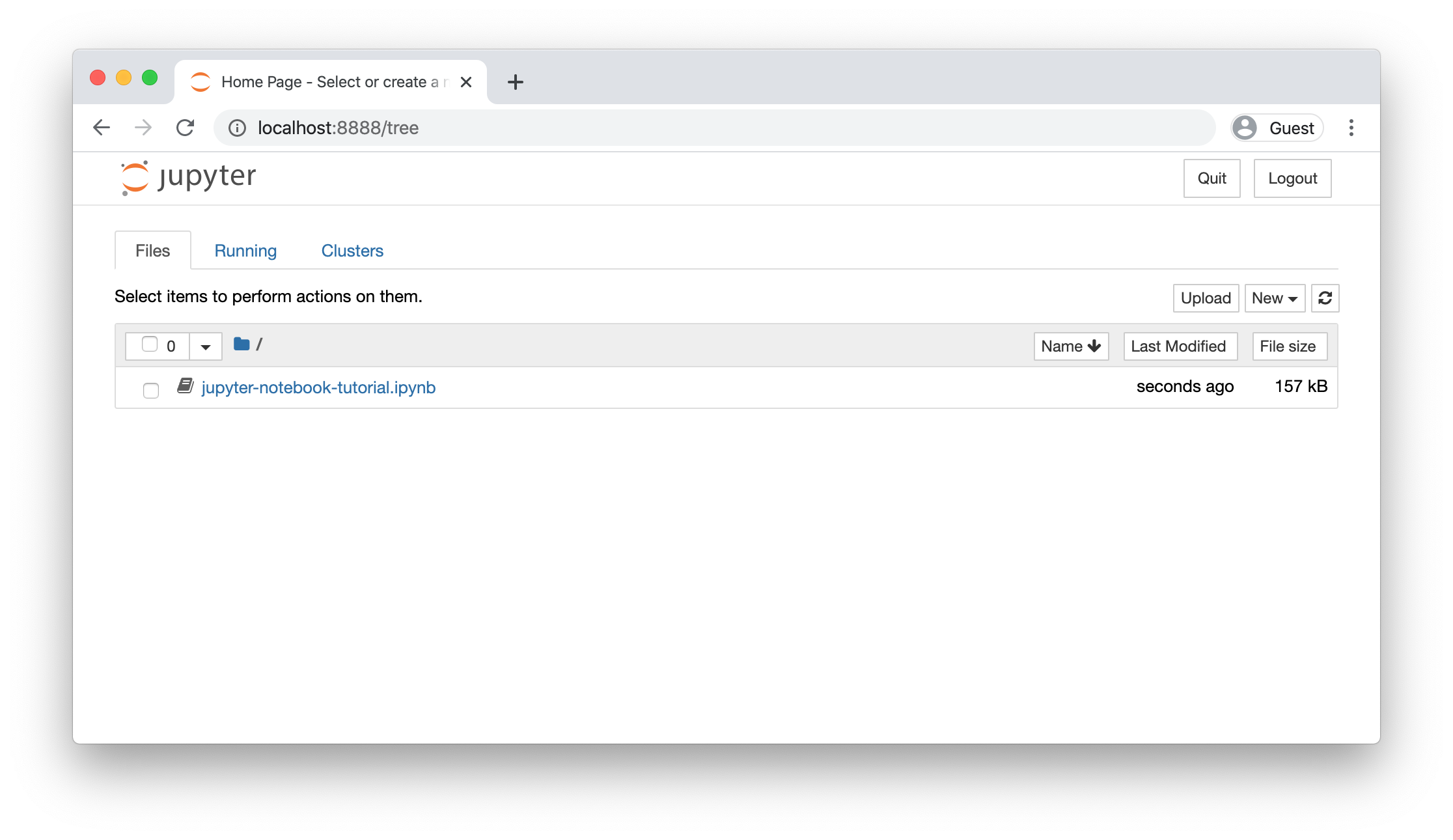
jupyter notebook. - This should automatically launch a notebook server at
http://localhost:8888. - If everything worked correctly, you should see a screen like the one shown below, showing all available notebooks in the current directory.
Remote setup
- Training a deep learning model often requires a lot of computational power, which is why we use specialized hardware, such as GPUs or TPUs. These processors can speed up training by many orders of magnitude compared to a CPU.
- Cloud computing services such as Amazon Web Services (AWS), Google Cloud, and Microsoft Azure allow us to access powerful computer instances on-demand: we can have just the right amount of power, when we need it! AI practitioners should know how to work with these remote computers in order to access the right hardware.
- Next, we’ll walk you through how to set up your own AWS instance.
Launching an EC2 instance
-
There are different types of AWS instances. We will use the
p2.xlargefor accelerated computing, which contains one NVIDIA K80 GPU.- Create an account here.
- Sign in into your account here.
- In the top right corner of the home page, click on the location name and set it to
US West (Oregon). This AWS region has instances with GPUs, and is cost-effective and offers good ping latency for folks on the west coast.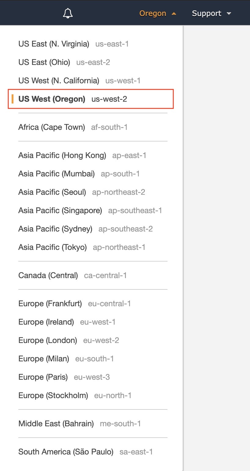
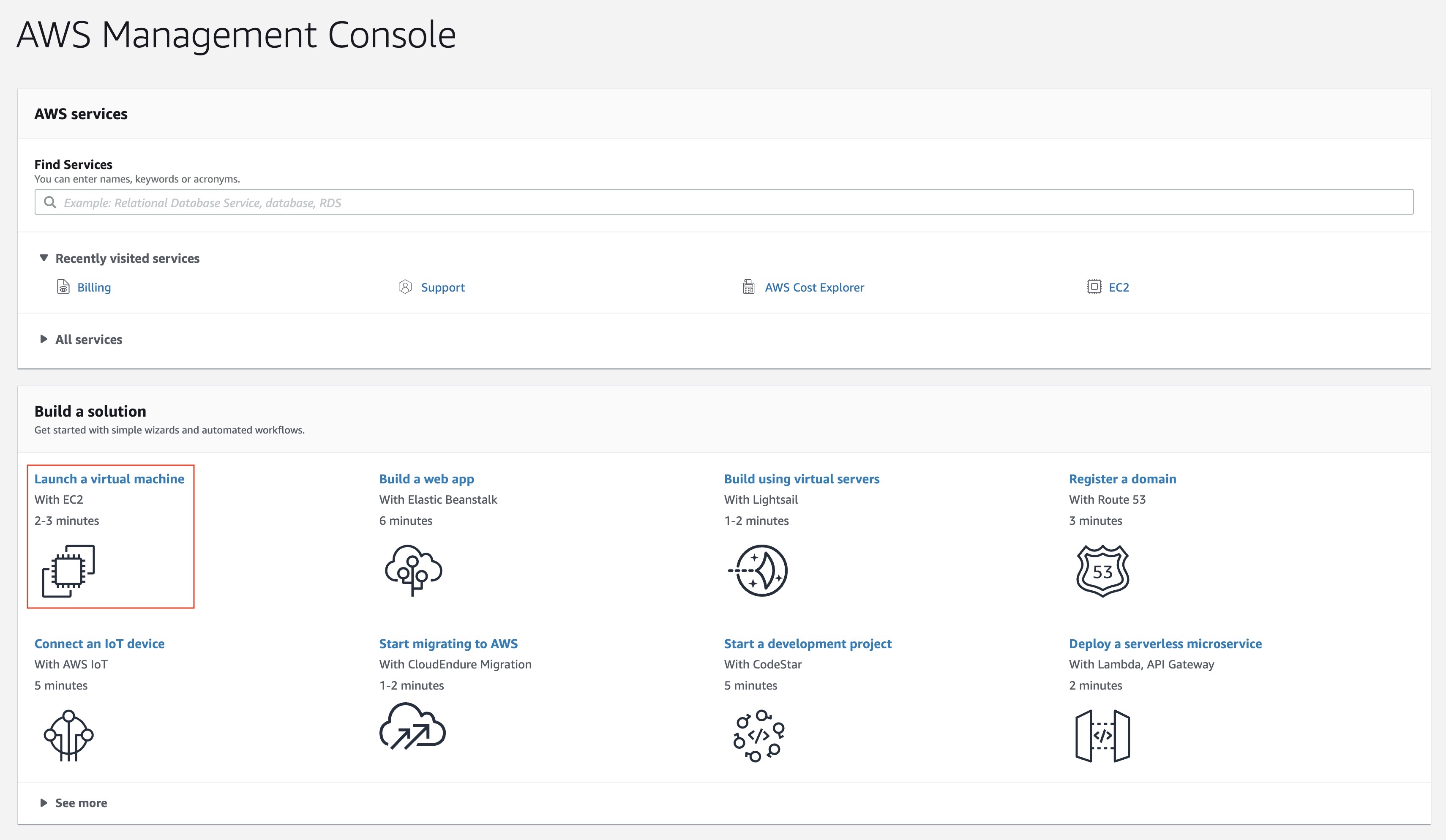
- After selecting the region, click on EC2 under the Compute list.
- In order to create an EC2 instance with a GPU, we’ll need to request a limit increase here.
- Choose Region as
US West (Oregon), Instance Type asAll P instances, and New limit value as4. - For use case, you can write something like “Training neural networks for your deep learning class”.
- AWS will contact you when your increase is approved: then, continue with the following steps. If you don’t want to wait, you can use a
t2.xlargeinstance, which is much slower because it doesn’t have GPUs.
- Choose Region as
- On the EC2 Dashboard view, click on the “Launch Instance” button.
- Search for and select the Deep Learning AMI (Ubuntu 16.04) Version 26.0. This AMI (Amazon Machine Image) comes with pre-installed deep learning frameworks such as TensorFlow, PyTorch or Keras.
- In the next page, select the
p2.xlargeinstance. Then, click on “Review and Launch”.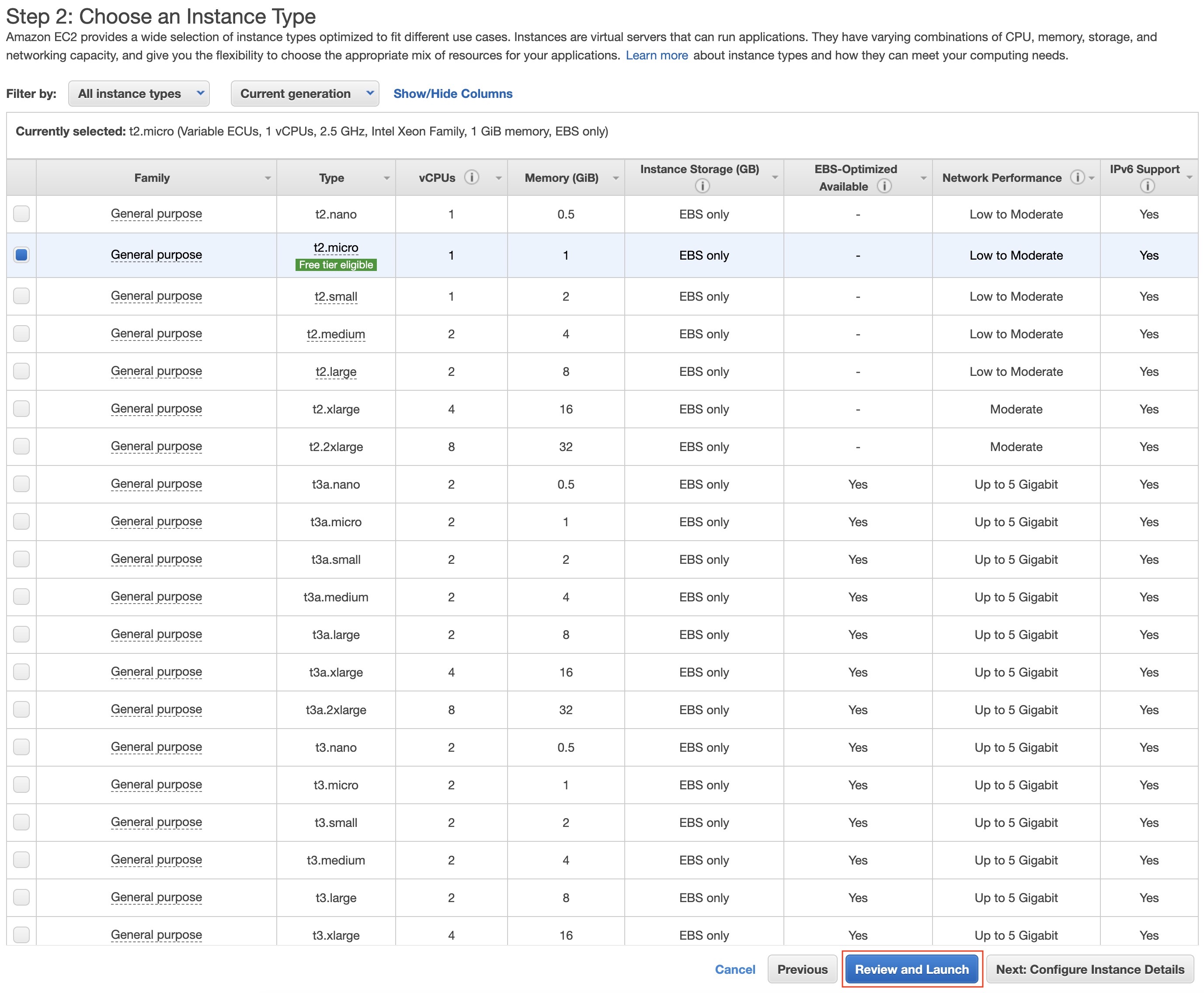
- Then, click on the blue button “Launch”.
- A pop-up window will appear asking for a key pair. You can either provide one or create one. If you create one, you should download it and keep it somewhere it won’t be deleted (if that happens, you won’t be able to access your instance anymore!).
- If you downloaded the key file, change its permissions in the terminal to user-only read and write. In Linux, this could be done with
chmod 400 PEM_FILENAMEwhere PEM_FILENAME is the file with the key. - After this, click on the blue button “Launch Instances”.
- Click on “View Instances” to check that it is “Running” and passed “2/2 status checks”. It will take some time to pass the checks but after that, you will be ready to ssh into the instance. Finally, note down the Public IP of the instance launched (it will be required in the next step).
- SSH into your instance with
ssh -i PEM_FILENAME ubuntu@PUBLIC_IP. - Your machine comes with many Conda environments pre-installed: each one is a Python environment with deep learning libraries already installed. Look at the README for how to use them. For this section, we can use a Tensorflow environment (
source activate tensorflow_p36).
Additional AWS Info
- VERY IMPORTANT! When you’re done using your instance, be sure to turn it off using the web interface! Otherwise your AWS account will be charged $0.90/hr for a
p2.xlargeinstance (see billing details below). - AWS bills instances by the minute, so make sure to turn off your machine (and save your data, if needed!) when you’re done using it.
Popular EC2 instances
- For prototyping or training small to moderately large networks, we recommend the
p2.xlarge/p2.8xlargeinstance. - For training large networks, the
p3.2xlarge/p3.16xlargecan be used, which utilizes one of the fastest GPUs on earth at the time of writing, the Nvidia Tesla V100 GPU. This instance can train networks much faster (but is also 3x more expensive!). - Here’s a quick comparison of the aforementioned EC2 instances:
| p2.xlarge | p2.8xlarge |
p3.2xlarge |
p3.16xlarge |
|
|---|---|---|---|---|
| GPUs | 1 (K80) | 8 (K80) | 1 (Tesla V100) | 8 (Tesla V100 w/ NVLink) |
| GPU Memory (GB) | 12 | 96 | 16 | 128 |
| vCPUs | 4 | 32 | 8 | 64 |
| RAM (GiB) | 61 | 488 | 61 | 488 |
| Network Bandwidth | High | 10 Gbps | Up to 10 Gbps | 25 Gbps |
| On-Demand Price/Hour* | $0.90 | $7.20 | $3.06 | $24.48 |
Launching Jupyter notebooks on a remote instance
Configuring Jupyter
- For most practical purposes, the default Jupyter configuration does the job well. But, if you wish to modify settings like the port over which your notebook is available, or secure your notebook with a password, follow on or simply move over to the next section.
-
Here’s how you can create a Jupyter configuration file, to override certain attributes. Before we begin, ssh into your instance with
ssh -i PATH_TO_PEM_FILE ubuntu@INSTANCE_IP_ADDRESSand follow these steps on your instance:- Generate a new Jupyter config file:
jupyter notebook --generate-config. - Edit
~/.jupyter/jupyter_notebook_config.pyusing your text editor of choice (viis a good default) and add the following at the beginning of the file (before all of the commented lines):
c = get_config() c.IPKernelApp.pylab = 'inline' c.NotebookApp.ip = '0.0.0.0' c.NotebookApp.open_browser = False c.NotebookApp.port = 8888 c.NotebookApp.token = '' c.NotebookApp.password = '' - Generate a new Jupyter config file:
Running Jupyter
- Whenever you want to start a Jupyter notebook, navigate to the directory you’re working in and run
jupyter notebook. - This will run a Jupyter notebook server on the default port
8888(unless you overrode the port in the above section) of your remote instance. You can also specify a port inline as a command line argument, sayjupyter notebook --port=8889, to run it on a different port (because you would like to run multiple notebook servers at the same time, for example).
Using Jupyter from your local browser
- We’ll need to set up port forwarding on your local machine so that your browser can communicate with your remote Jupyter server.
-
Choose an open local port
8888is probably fine assuming you’re not running any other Jupyter servers on your local machine, but we’ll be using port9000), and run the following command to start forwarding your local port9000to port8888of the remote instance:ssh -i PATH_TO_PEM_FILE -fNL 9000:localhost:8888 ubuntu@INSTANCE_IP_ADDRESS - Folks on your team who would like to connect to a Jupyter notebook on your remote instance will need to run that command on their local machine first.
- In your local browser, navigate to the URL
localhost:9000and you should arrive at the Jupyter dashboard. From there, you can use the “New” button near the top right of the dashboard to create a new notebook, text file, directory, or terminal window, and you can use the “Upload” button to transfer files from your local machine to your instance. - For TensorFlow projects, you’ll likely want to use the
tensorflow_p36conda environment. For PyTorch projects, you can use thepytorch_p36environment.
screen/tmux
-
If you want to persist processes you launch from the command line on your instance across SSH sessions so that you can disconnect without shutting down your Jupyter server, you can use either
screenortmux. These are good utilities to know about for managing terminals on remote servers – here we’ll describe an example workflow usingtmux.- Create a new
tmuxsession on your EC2 instance usingtmux. - Navigate to the directory you’ll be working from and start your Jupyter server with
jupyter notebook - Detach from your
tmuxsession withCTRL-B D(hold the Control and B keys, release both, and press the D key). - Your Jupyter server will now stay up even if you log out from your instance. To verify this, logout with
exitorCTRL-D. - SSH back into your instance.
- Re-attach to your tmux session using
tmux attachto verify that your Jupyter server is still running.
- Create a new
References
- CS231n Software Setup for the basics.
- CS230 Section 2 for AWS instance setup details and
screen/tmux. - Python Numpy Tutorial (with Jupyter and Colab) for details on Jupyter and Colab Notebooks.
- What is the python requirements.txt? for details on
requirements.txtandpip freeze.