Primers • Expression for Partial Gradient of Batchnorm
- Introduction
- Batch Normalization
- Notation
- Chain Rule Primer
- Problem Statement
- Partial Derivatives
- Recap
- Python Implementation
- Key Takeaways
- References
Introduction
-
This topic was mostly inspired by the question in Assignment 2 of Stanford’s CS231n which requires you to derive an expression for the gradient of the batchnorm layer. Here, we explore the derivation in detailed steps and provide some sample code.
- The overall task in the assignment is to implement a Batch Normalization layer in a fully-connected net with a forward and backward pass. While the forward pass is relatively simple since it only requires standardizing the input features (zero mean and unit standard deviation). The backwards pass, on the other hand, is a bit more involved. It can be done in 2 different ways:
- Staged computation: break up the function into several parts, derive local gradients for each of these parts, and finally group them together by multiplying them per the chain rule.
- Interested in the staged computation method? head over to Backward Pass of Batchnorm!
- Gradient derivation: do a “pen and paper” derivation of the gradient with respect to the inputs.
- Staged computation: break up the function into several parts, derive local gradients for each of these parts, and finally group them together by multiplying them per the chain rule.
- It turns out that second option is faster, albeit nastier and you will possibly need to endure a bit of a struggle to get it done.
- The aim behind this post is to offer a clear explanation of the derivation along with the thought process so as to build insight and intuition.
Batch Normalization
- Batch Normalization is a technique to provide any layer in a Neural Network with inputs that are zero mean/unit variance - and this is basically what they like! But Batchnorm consists of one more step which makes this algorithm really powerful. Let’s take a look at the Batchnorm Algorithm:
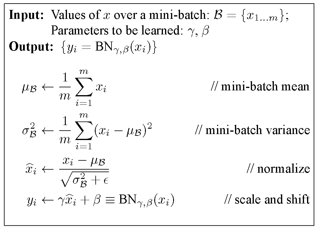
- Looking at the last line of the algorithm, after normalizing the input \(x\), the result is squashed through a linear function with parameters \(\gamma\) and \(\beta\). These are learnable parameters of the Batchnorm Layer which offer the model an extra degree of freedom in terms of letting it get back to its original data-distribution (the one that gets fed in as input to the batchnorm layer) if it doesn’t like the zero mean/unit variance input that Batchnorm aspires to set up.
- Thus, if \(\gamma = \sqrt{\sigma(x)}\) and \(\beta = \mu(x)\), the original activation is restored.
- This is what makes Batchnorm really powerful. Put simply, we initialize the Batchnorm Parameters to transform the input to zero mean/unit variance distributions but during training Batchnorm can learn that another distribution might serve our purpose better.
The “Batch” in Batchnorm stems from the fact that we’re transforming the input based on the statistics for only a batch (i.e., a part) of the entire training set at a time, rather than going at it at a per-sample granularity or the entire training set.
- To learn more about Batchnorm, read “Batch Normalization: Accelerating Deep Network Training by Reducing Internal Covariate Shift” (2015) by Ioffe and Szegedy. Also, here is a visual explanation of Batchnorm from Stanford’s CS231n.
Notation
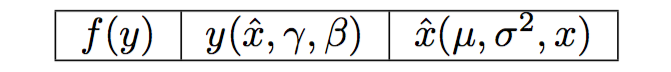
- Let’s start with some notation.
| \(f\) | the final output of the network |
| \(y\) | linear transformation which scales \(x\) by \(\gamma\) and adds \(\beta\) |
| \(\hat{x}\) | normalized inputs |
| \(\mu\) | batch mean |
| \(\sigma^2\) | batch variance |
Chain Rule Primer
- Make sure to go through “Primer: Chain Rule for Backprop” before you proceed - understanding of the chain rule is necessary for the later sections.
Problem Statement
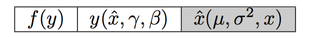
- The below table shows you the inputs to each function and will help with the future derivation.
-
Goal: Find the partial derivatives with respect to the inputs, that is \(\dfrac{\partial f}{\partial \gamma}\), \(\dfrac{\partial f}{\partial \beta}\) and \(\dfrac{\partial f}{\partial x_i}\).
-
Methodology: derive the gradient with respect to the centered inputs \(\hat{x}_i\) (which requires deriving the gradient w.r.t \(\mu\) and \(\sigma^2\)) and then use those to derive one for \(x_i\).
Partial Derivatives
- Let’s begin by traversing the above table from left to right. At each step, we’ll derive the gradient with respect to the inputs in the cell.
Cell 1
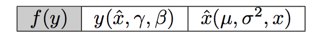
- Let’s compute \(\dfrac{\partial f}{\partial y_i}\). It actually turns out we don’t need to compute this derivative since we already have it - it’s the upstream derivative (referred to as
doutin Stanford’s CS231n and is given to us as an input to the function in Assignment 2).
Cell 2
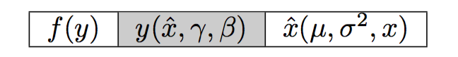
- Let’s work on cell 2 now. We note that \(y\) is a function of \(\hat{x}\), \(\gamma\) and \(\beta\), so let’s compute the gradient with respect to each one.
Starting with \(\gamma\) and using the chain rule:
\[\begin{eqnarray} \frac{\partial f}{\partial \gamma} &=& \frac{\partial f}{\partial y_i} \cdot \frac{\partial y_i}{\partial \gamma} \qquad \\ &=& \boxed{\sum\limits_{i=1}^m \frac{\partial f}{\partial y_i} \cdot \hat{x}_i} \end{eqnarray}\]- Notice that we sum from \(1 \rightarrow m\) because we’re working with batches! If you’re worried you wouldn’t have caught that, make sure to perform dimension-checks at every step of the process.
- The gradient with respect to a variable should be of the same size as that same variable so if those two clash, it should tell you you’ve done something wrong.
Moving on to \(\beta\) we compute the gradient as follows:
\[\begin{eqnarray} \frac{\partial f}{\partial \beta} &=& \frac{\partial f}{\partial y_i} \cdot \frac{\partial y_i}{\partial \beta} \qquad \\ &=& \boxed{\sum\limits_{i=1}^m \frac{\partial f}{\partial y_i}} \end{eqnarray}\]and finally \(\hat{x}_i\):
\[\begin{eqnarray} \frac{\partial f}{\partial \hat{x}_i} &=& \frac{\partial f}{\partial y_i} \cdot \frac{\partial y_i}{\partial \hat{x}_i} \qquad \\ &=& \boxed{\frac{\partial f}{\partial y_i} \cdot \gamma} \end{eqnarray}\]- Up to now, things are relatively simple and we’ve already most of the work. We can’t compute the gradient with respect to \(x_i\) just yet though.
Cell 3
- Let’s start with \(\mu\). Since \(\sigma^2\) is a function of \(\mu\), we need to add its contribution to the partial - (the missing partials are highlighted in red):
- Let’s compute the missing partials one at a time.
- From
- we compute:
- and from
- we calculate:
- We’re missing the partial with respect to \(\sigma^2\) and that is our next variable, so let’s get to it and come back and plug it in here.
- In the expression of the partial:
-
Let’s focus on \(\dfrac{\partial \hat{x}}{\partial \sigma^2}\). Rewrite \(\hat{x}\) to make its derivative easier to compute:
\[\hat{x}_i = (x_i - \mu)(\sqrt{\sigma^2 + \epsilon})^{-0.5}\]- Since \((x_i - \mu)\) is a constant:
- With all that out of the way, let’s plug everything back in our previous partial!
- Finally, we have:
Note that there’s a summation in \(\dfrac{\partial \hat{x}_i}{\partial \mu}\) because we want the dimensions to add up with respect to dfdmean and not dxnormdmean.
- We finally arrive at the last variable \(x\). Again adding the contributions from any parameter containing \(x\) we obtain:
- The missing pieces are easy to compute at this point:
-
Thus, our final gradient is:
\[\frac{\partial f}{\partial x_i} = \bigg(\frac{\partial f}{\partial \hat{x}_i} \cdot \dfrac{1}{\sqrt{\sigma^2 + \epsilon}}\bigg) + \bigg(\frac{\partial f}{\partial \mu} \cdot \dfrac{1}{m}\bigg) + \bigg(\frac{\partial f}{\partial \sigma^2} \cdot \dfrac{2(x_i - \mu)}{m}\bigg)\]- Note the following trick:
- Let’s plug in the partials and see if we can simplify the expression some more:
- Finally, we factorize by the \(\frac{(\sigma^2 + \epsilon)^{-0.5}}{m}\) factor and obtain:
Recap
- Let’s summarize the final equations we derived. Using \(\dfrac{\partial f}{\partial \hat{x}_i} = \dfrac{\partial f}{\partial y_i} \cdot \gamma\), we obtain the gradient with respect to our inputs:
Python Implementation
- Here’s an example Python implementation using the equations we derived. To compress the code a bit further, you can get creative with shorter variable names - this can also help accommodate the recommended \(80\) characters limit in Stanford’s CS231n.
def batchnorm_backward(dout, cache):

	N, D = dout.shape
	x_mu, inv_var, x_hat, gamma = cache

	# intermediate partial derivatives
	dxnorm = dout * gamma

	# final partial derivatives
	dx = (1. / N) * inv_var * (N*dxnorm - np.sum(dxnorm, axis=0)
		- x_hat*np.sum(dxnorm*x_hat, axis=0))
	dbeta = np.sum(dout, axis=0)
	dgamma = np.sum(x_hat*dout, axis=0)

	return dx, dgamma, dbeta
- This version of the Batchnorm backward pass can give you a significant boost in speed. Timing both versions, you observe a superb \(3x\) increase in speed!
Key Takeaways
- Learned how to use the chain rule in a staged manner to derive the expression for the gradient of the batch norm layer.
- Saw how a smart simplification can help significantly reduce the complexity of the expression for
dx. - Finally, implemented it as part of the backward pass with Python. This version of the function resulted in a \(3x\) speed increase!
References
- Deriving the Gradient for the Backward Pass of Batch Normalization was the major inspiration behind this post.
- Clément Thorey’s Blog offers a similar tutorial that covers the gradient derivation of Batchnorm.