Primers • Partial Gradient of Batchnorm
- Introduction
- Batch Normalization
- Notation
- Chain Rule Primer
- Computational Graph of the Batch Normalization Layer
- Breaking down the forward pass into small steps
- Putting it together
- Naive implementation of the backward pass
- References
Introduction
-
This topic was mostly inspired by the question in Assignment 2 of Stanford’s CS231n which requires you to derive an expression for the gradient of the batchnorm layer. Here, we explore the derivation in detailed steps and provide some sample code.
- The overall task in the assignment is to implement a Batch Normalization layer in a fully-connected net with a forward and backward pass. While the forward pass is relatively simple since it only requires standardizing the input features (zero mean and unit standard deviation). The backwards pass, on the other hand, is a bit more involved. It can be done in 2 different ways:
- Staged computation: break up the function into several parts, derive local gradients for each of these parts, and finally group them together by multiplying them per the chain rule.
- Gradient derivation: do a “pen and paper” derivation of the gradient with respect to the inputs.
- Interested in the gradient derivation method? head over to Expression for Backward Pass of Batchnorm”!
- It turns out that second option is faster, albeit nastier and you will possibly need to endure a bit of a struggle to get it done.
- The goal of this topic is to explain the gradient flow through the Batchnorm layer using its computation graph (also called the “circuit” representation).
Batch Normalization
- Batch Normalization is a technique to provide any layer in a Neural Network with inputs that are zero mean/unit variance - and this is basically what they like!
- Batchnorm does consist of one more step which makes this algorithm really powerful. Let’s take a look at the Batchnorm Algorithm:
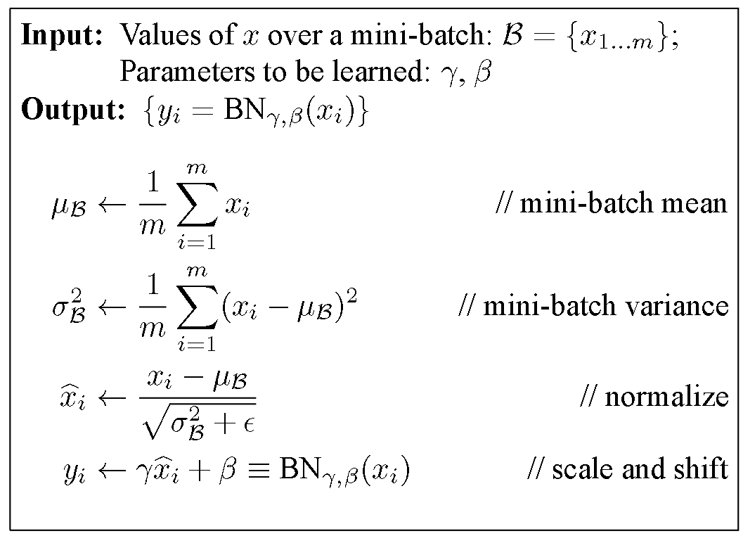
- Looking at the last line of the algorithm, after normalizing the input \(x\), the result is squashed through a linear function with parameters \(\gamma\) and \(\beta\). These are learnable parameters of the Batchnorm Layer which offer the model an extra degree of freedom in terms of letting it get back to its original data-distribution (the one that gets fed in as input to the batchnorm layer) if it doesn’t like the zero mean/unit variance input that Batchnorm aspires to set up.
- Thus, if \(\gamma = \sqrt{\sigma(x)}\) and \(\beta = \mu(x)\), the original activation is restored.
- This is what makes Batchnorm really powerful. Put simply, we initialize the Batchnorm Parameters to transform the input to zero mean/unit variance distributions but during training Batchnorm can learn that another distribution might serve our purpose better.
The “Batch” in Batchnorm stems from the fact that we’re transforming the input based on the statistics for only a batch (i.e., a part) of the entire training set at a time, rather than going at it at a per-sample granularity or the entire training set.
- To learn more about Batchnorm, read “Batch Normalization: Accelerating Deep Network Training by Reducing Internal Covariate Shift” (2015) by Ioffe and Szegedy. Also, here is a visual explanation of Batchnorm from Stanford’s CS231n.
Notation
- Let’s start with some notation.
| \(f\) | the final output of the network |
| \(y\) | linear transformation which scales \(x\) by \(\gamma\) and adds \(\beta\) |
| \(\hat{x}\) | normalized inputs |
| \(\mu\) | batch mean |
| \(\sigma^2\) | batch variance |
Chain Rule Primer
- Make sure to go through “Primer: Chain Rule for Backprop” before you proceed - understanding of the chain rule is necessary for the later sections.
Computational Graph of the Batch Normalization Layer
- Computational graphs help graphically interpret the forward and backward passes of a function. They are a good way to visualize the computational flow of fairly complex functions by small, piecewise differentiable sub-functions.
- The figure below shows the computational graph of the Batchnorm layer, illustrating the forward and backward pass.
- From left to right, the black arrows represent the forward pass. The inputs are our matrix \(X\) and \(\gamma, \beta\) as vectors.
- From right to left, the red arrows represent the backward pass which distributes the gradient from the upward layer to \(\gamma\) and \(\beta\) and all the way back to the input.
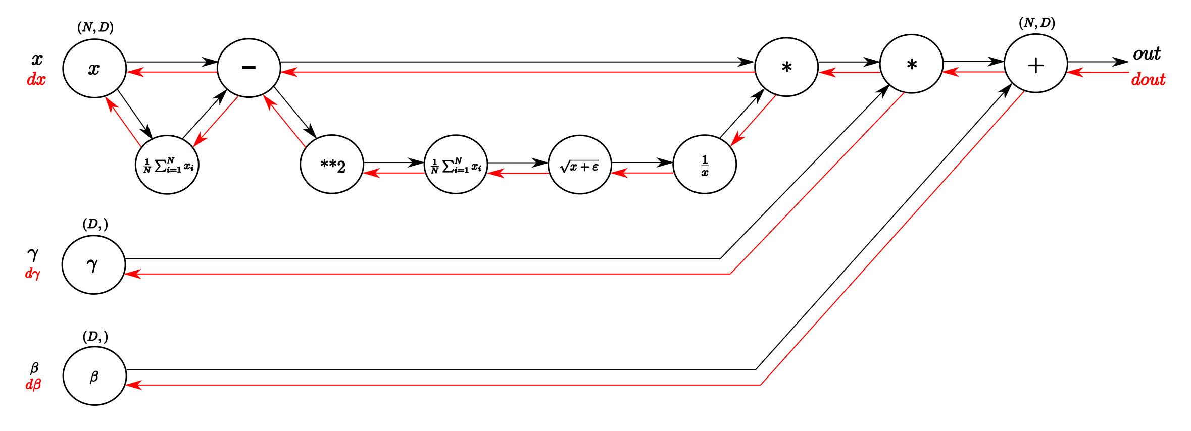
- The forward pass is straightforward to interpret. From input \(x\), we calculate the mean of every dimension in the feature space and then subtract this vector of mean values from every training example.
- Following the lower branch, we calculate the per-dimension variance and with that the entire denominator of the normalization equation. Next, we invert it and multiply it with difference of inputs and means and we have \(x_{norm}\).
- The last two blobs on the right perform the squashing by scaling \(x_{norm}\) with \(\gamma\) and shifting the result by \(\beta\). This represents our batch-normalized output.
A vanilla implementation of the forward pass might look like this:
def batchnorm_forward(x, gamma, beta, eps):
    N, D = x.shape

    # compute the sample mean and variance from mini-batch statistics
    # using minimal-num-of-operations-per-step policy to ease the backward pass

    # (1) mini-batch mean by averaging over each sample (N) in a minibatch
    # for a particular column / feature dimension (D)
    mean = x.mean(axis = 0) # (D,)
    # can also do mean = 1./N * np.sum(x, axis = 0)

    # (2) subtract mean vector of every training example
    dev_from_mean = x - mean # (N,D)

    # (3) following the lower branch for the denominator
    dev_from_mean_sq = dev_from_mean ** 2 # (N,D)

    # (4) mini-batch variance
    var = 1./N * np.sum(dev_from_mean_sq, axis = 0) # (D,)
    # can also do var = x.var(axis = 0)

    # (5) get std dev from variance, add eps for numerical stability
    stddev = np.sqrt(var + eps) # (D,)

    # (6) invert the above expression to make it the denominator
    inverted_stddev = 1./stddev # (D,)

    # (7) apply normalization
    # note that this is an element-wise multiplication using broad-casting
    x_norm = dev_from_mean * inverted_stddev # also called z or x_hat (N,D)

    # (8) apply scaling parameter gamma to x
    scaled_x = gamma * x_norm # (N,D)

    # (9) shift x by beta
    out = scaled_x + beta # (N,D)

    # cache values for backward pass
    cache = {'mean': mean, 'stddev': stddev, 'var': var, 'gamma': gamma,
             'beta': beta, 'eps': eps, 'x_norm': x_norm, 'dev_from_mean': dev_from_mean,
             'inverted_stddev': inverted_stddev, 'x': x}

    return out, cache
- While the above code snippet shows the training mode of the forward pass of Batchnorm, a practical implementation of Batchnorm should be able to handle a different forward pass for test mode by calculating the running mean and variance. However, for the purposes of explaining the backward pass, the above simplified version of forward pass should do just fine!
- In
cache, we make a copy of certain important intermediary variables computed during the forward pass that come in handy during the backward pass.
Breaking down the forward pass into small steps
- Note that in the comments of the above code snippet, we’ve already numbered the computational steps – this helps tackle the backward pass piece-wise and thus, makes it tractable. Note that backprop follows these steps in reverse order, as we are literally back-passing through the computational graph.
- Let’s dive into a more detailed step-by-step look at the computations involved in the backward pass.
Step 9
- The figure below shows the backward pass through the last summation gate of the Batchnorm layer. Next to each forward/backward term, the dimensions of the corresponding term are enclosed in brackets.
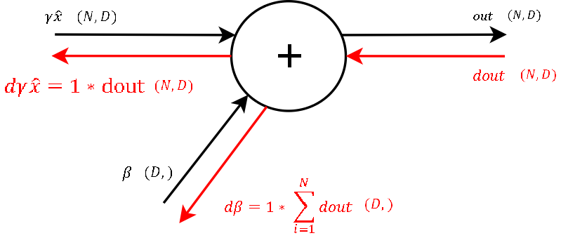
- Recall that the derivative of a function \(f = x + y\) with respect to any of these two variables is 1. This means to channel a gradient through a summation gate, we only need to multiply by 1. For our final loss evaluation, we sum the gradient of all samples in the batch.
- Through this operation, we also get a vector of gradients with the correct shape for \(\beta\). So after the first step of backprop we already got the gradient for one learnable parameter \(\beta\).
Step 8
- Next, let’s backward pass through the multiplication gate of the normalized input and the \(\gamma\) vector, as shown below:
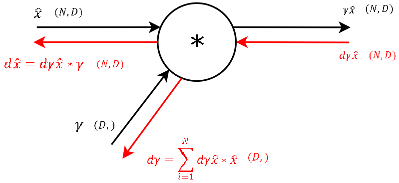
- For any function \(f = x * y\) the derivative with respect to one of the inputs is simply just the other input variable. This also means, that for this step of the backward pass we need the variables used in the forward pass of this gate (stored in the forward pass’s cache).
- We get the gradients of the two inputs of these gates by applying chain rule which essentially enables us to obtain the downstream gradient by multiplying the local gradient with the upstream gradient.
- For \(\gamma\), as for \(\beta\) in step 9, we need to sum up the gradients over dimension \(N\). So we now have the gradient for the second learnable parameter of the Batchnorm layer \(\gamma\) and “only” need to backprop the gradient to the input \(x\), so that we then can backpropagate the gradient to any layer further downwards.
Step 7
- This step during the forward pass was the final step of the normalization combining the two branches (nominator and denominator) of the computational graph. During the backward pass, we will calculate the gradients that will flow separately through these two branches backwards.
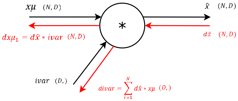
- It’s basically the exact same operation, so lets not waste much time and continue. The two needed variables
dev_from_meanandinverted_stddevfor this step are also storedcachevariable we pass to the backprop function. (And again: This is one of the main advantages of computational graphs. Splitting complex functions into a handful of simple basic operations (which can be potentially repeated throughout your graph - thus, making the process easy!)
Step 6
- This is a “one input-one output” node where, during the forward pass, we inverted the input (square root of the variance).
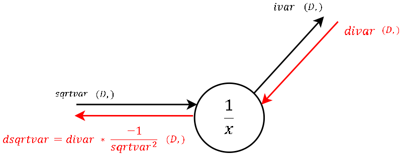
- The local gradient is visualized in the image and should not be hard to derive by hand. Multiplied by the gradient from above is what we channel to the next step.
stddevis also one of the variables stored in the cache.
Step 5
- Again “one input-one output”. This node calculates during the forward pass the denominator of the normalization.
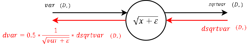
- The calculation of the derivative of the local gradient is little magic and should need no explanation.
varandepsare also passed in thecache.
Step 4
- Also a “one input-one output” node. During the forward pass the output of this node is the variance of each feature \(\text{d for d in [1…D]}\).
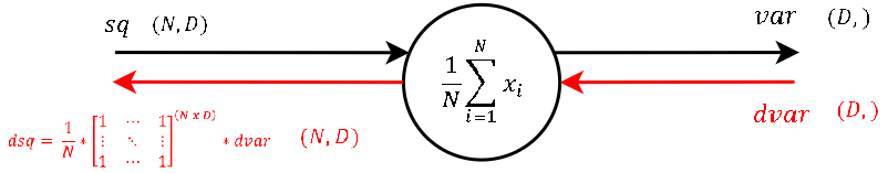
- The calculation of the derivative of this steps local gradient might look unclear at the very first glance. But it’s not that hard at the end. Let’s recall that a normal summation gate (see step 9) during the backward pass only transfers the gradient unchanged and evenly to the inputs.
- With that in mind, it should not be that hard to conclude, that a column-wise summation during the forward pass, during the backward pass means that we evenly distribute the gradient over all rows for each column.
- We create a matrix of ones with the same shape as the input
dev_from_mean_sqof the forward pass, divide it element-wise by the number of rows (thats the local gradient) and multiply it by the gradient from above.
Step 3
- This node outputs the square of its input, which during the forward pass was a matrix containing the input \(x\) subtracted by the per-feature
mean.
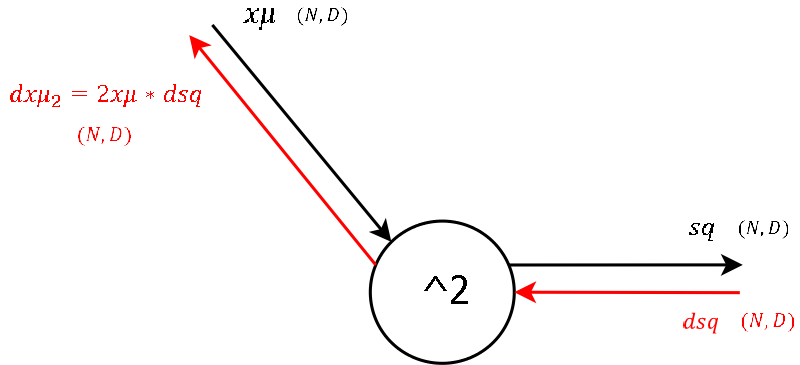
- The derivative of the local gradient for this step is mostly obvious.
Step 2
- This gate has two inputs-two outputs. This node subtracts the per-feature mean row-wise of each training sample \(\text{n for n in [1…N]}\) during the forward pass.
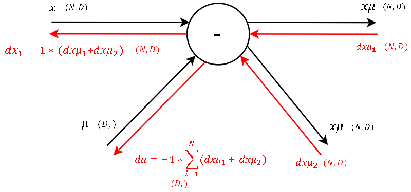
- One of the definitions of backprogatation and computational graphs is, that whenever we have two gradients coming to one node, we simply add them up. Knowing this, the rest is little magic as the local gradient for a subtraction is as hard to derive as for a summation.
- Note that for
meanwe have to sum up the gradients over the dimension \(N\) (as we did earlier for \(\gamma\) and \(\beta\)).
Step 1
- The function of this node is exactly the same as of step 4. Only that during the forward pass the input was \(x\) - the input to the Batchnorm layer and the output here is
mean, a vector that contains the per-feature mean.
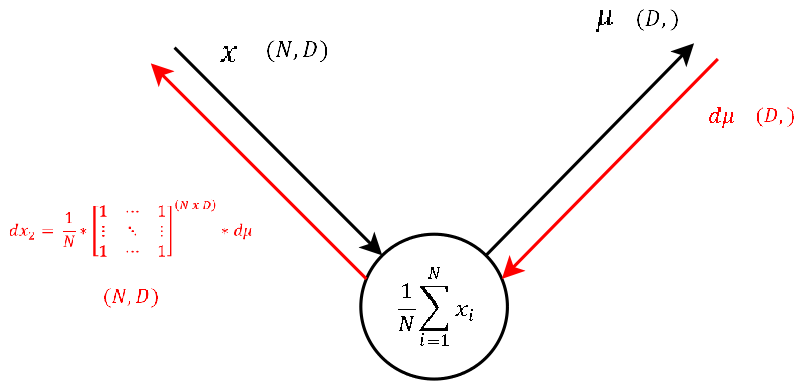
- As this node executes the exact same operation as the one explained in step 4, also the backpropagation of the gradient looks the same. So let’s continue to the last step.
Step 0 - Arriving at the input
- We’re at the very end! All we have to do is to sum up the gradients
dx1anddx2to get the final gradientdx.
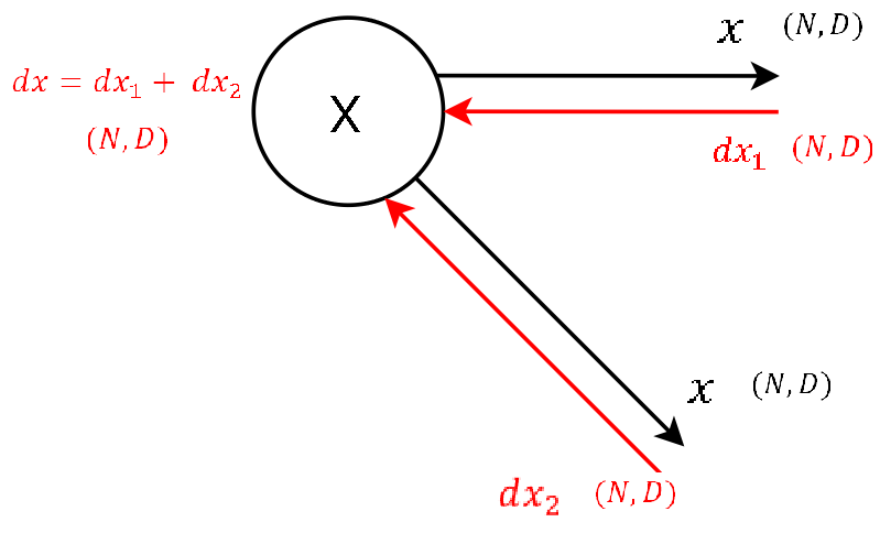
- This matrix contains the gradient of the loss function with respect to the input of the Batchnorm layer. This gradient
dxis also what we give as input to the backward pass of the next layer, as for this layer we receivedoutfrom the layer above.
Putting it together
Packing together our steps above, here’s an implementation of the backward pass in code:
def batchnorm_backward(dout, cache):
    # convention used is downstream gradient = local gradient * upstream gradient

    # extract all relevant params
    beta, gamma, x_norm, var, eps, stddev, dev_from_mean, inverted_stddev, x, mean, axis = \
    cache['beta'], cache['gamma'], cache['x_norm'], cache['var'], cache['eps'], \
    cache['stddev'], cache['dev_from_mean'], cache['inverted_stddev'], cache['x'], \
    cache['mean'], cache['axis']

    # get the num of training examples and dimensionality of the input (num of features)
    N, D = dout.shape # can also use x.shape

    # (9)
    dbeta = np.sum(dout, axis=axis)
    dscaled_x = dout

    # (8)
    dgamma = np.sum(x_norm * dscaled_x, axis=axis)
    dx_norm = gamma * dscaled_x

    # (7)
    dinverted_stddev = np.sum(dev_from_mean * dx_norm, axis=0)
    ddev_from_mean = inverted_stddev * dx_norm

    # (6)
    dstddev = -1/(stddev**2) * dinverted_stddev

    # (5)
    dvar = (0.5) * 1/np.sqrt(var + eps) * dstddev

    # (4)
    ddev_from_mean_sq = 1/N * np.ones((N,D)) * dvar # variance of mean is 1/N

    # (3)
    ddev_from_mean += 2 * dev_from_mean * ddev_from_mean_sq

    # (2)
    dx = 1 * ddev_from_mean
    dmean = -1 * np.sum(ddev_from_mean, axis=0)

    # (1)
    dx += 1./N * np.ones((N,D)) * dmean

    return dx, dgamma, dbeta
Naive implementation of the backward pass
- Note: This is the “naive” implementation of the backward pass. There exists an alternative implementation, which is much faster, but the naive implementation is way better for the purpose of understanding backprop through the Batchnorm layer.
- The faster gradient derivation approach offers a detailed treatment of the alternative (faster) implementation.
References
- Understanding the backward pass through Batch Normalization Layer was the major inspiration behind this post.