Primers • Xavier Initialization
- The importance of effective initialization
- The problem of exploding or vanishing gradients
- Visualizing the effects of different initializations
- How to find appropriate initialization values
- Xavier initialization
- Derivation: Xavier initialization
- Further Reading
- Citation
The importance of effective initialization
- To build a machine learning algorithm, usually you would define an architecture (for e.g., Logistic regression, Support Vector Machine, Neural Network) and train it to learn parameters. Here is a common training process for neural networks:
- Initialize the parameters.
- Choose an optimization algorithm.
- Repeat these steps:
- Forward propagate an input.
- Compute the cost function.
- Compute the gradients of the cost with respect to parameters using backpropagation.
- Update each parameter using the gradients, according to the optimization algorithm.
- Then, given a new data point, you can use the model to predict its class.
- The initialization step can be critical to the model’s ultimate performance, and it requires the right method. To illustrate this, think about what you would notice about the gradients and weights when the initialization method is zero?
Initializing all the weights with zeros leads the neurons to learn the same features during training.
- In fact, any constant initialization scheme will perform very poorly. Consider a neural network with two hidden units, and assume we initialize all the biases to 0 and the weights with some constant \(\alpha\). If we forward propagate an input \((x_1,x_2)\) in this network, the output of both hidden units will be \(relu(\alpha x_1 + \alpha x_2)\). Thus, both hidden units will have identical influence on the cost, which will lead to identical gradients. Thus, both neurons will evolve symmetrically throughout training, effectively preventing different neurons from learning different things.
- Now, let’s ponder about what you would notice about the loss curve when you initialize weights with values too small or too large?
Despite breaking the symmetry, initializing the weights with values (i) too small or (ii) too large leads respectively to (i) slow learning or (ii) divergence.
- Choosing proper values for initialization is necessary for efficient training. We will investigate this further in the next section.
The problem of exploding or vanishing gradients
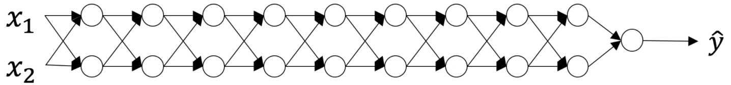
- Consider this 9-layer neural network.
-
At every iteration of the optimization loop (forward, cost, backward, update), we observe that backpropagated gradients are either amplified or minimized as you move from the output layer towards the input layer. This result makes sense if you consider the following example.
-
Assume all the activation functions are linear (identity function). Then the output activation is:
\[\hat{y} = a^{[L]} = W^{[L]}W^{[L-1]}W^{[L-2]}\dots W^{[3]}W^{[2]}W^{[1]}x\]- where \(L=10\) and \(W^{[1]}\), \(W^{[2]}\), \(\dots\), \(W^{[L-1]}\) are all matrices of size \((2,2)\) because layers \([1]\) to \([L-1]\) have 2 neurons and receive 2 inputs. With this in mind, and for illustrative purposes, if we assume \(W^{[1]} = W^{[2]} = \dots = W^{[L-1]} = W\), the output prediction is \(\hat{y} = W^{[L]}W^{L-1}x\) (where \(W^{L-1}\) takes the matrix \(W\) to the power of \(L-1\), while \(W^{[L]}\) denotes the \(L^{th}\) matrix).
-
What would be the outcome of initialization values that were too small, too large or appropriate?
Case 1: A too-large initialization leads to exploding gradients
- Consider the case where every weight is initialized slightly larger than the identity matrix.
- This simplifies to \(\hat{y} = W^{[L]}1.5^{L-1}x\), and the values of \(a^{[l]}\) increase exponentially with \(l\). When these activations are used in backward propagation, this leads to the exploding gradient problem. That is, the gradients of the cost with the respect to the parameters are too big. This leads the cost to oscillate around its minimum value.
Case 2: A too-small initialization leads to vanishing gradients
- Similarly, consider the case where every weight is initialized slightly smaller than the identity matrix.
- This simplifies to \(\hat{y} = W^{[L]}0.5^{L-1}x\), and the values of the activation \(a^{[l]}\) decrease exponentially with \(l\). When these activations are used in backward propagation, this leads to the vanishing gradient problem. The gradients of the cost with respect to the parameters are too small, leading to convergence of the cost before it has reached the minimum value.
- All in all, initializing weights with inappropriate values will lead to divergence or a slow-down in the training of your neural network. Although we illustrated the exploding/vanishing gradient problem with simple symmetrical weight matrices, the observation generalizes to any initialization values that are too small or too large.
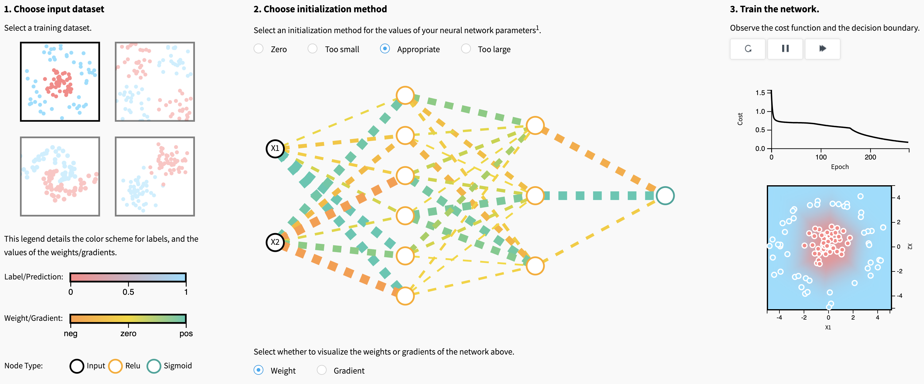
Visualizing the effects of different initializations
- All deep learning optimization methods involve an initialization of the weight parameters.
- Let’s explore the first visualization in this article to gain some intuition on the effect of different initializations. Two questions come to mind:
- What makes a good or bad initialization? How can different magnitudes of initializations lead to exploding and vanishing gradients?
- If we initialize weights to all zeros or the same value, what problem arises?
- Visualizing the effects of different initializations:
How to find appropriate initialization values
- To prevent the gradients of the network’s activations from vanishing or exploding, we will stick to the following rules of thumb:
- The mean of the activations should be zero.
- The variance of the activations should stay the same across every layer.
- Under these two assumptions, the backpropagated gradient signal should not be multiplied by values too small or too large in any layer. It should travel to the input layer without exploding or vanishing.
- More concretely, consider a layer \(l\). Its forward propagation is:
- We would like the following to hold:
- Ensuring zero-mean and maintaining the value of the variance of the input of every layer guarantees no exploding/vanishing signal, as we’ll explain in a moment. This method applies both to the forward propagation (for activations) and backward propagation (for gradients of the cost with respect to activations).
Xavier initialization
- The recommended initialization is Xavier initialization (or one of its derived methods), for every layer \(l\):
-
In other words, all the weights of layer ll are picked randomly from a normal distribution with mean \(\mu = 0\) and variance \(\sigma^2 = \frac{1}{n^{[l-1]}}\) where \(n^{[l-1]}n\) is the number of neuron in layer \(l-1\). Biases are initialized with zeros.
-
You can find the theory behind this visualization in Glorot et al. (2010). The next section presents the mathematical justification for Xavier initialization and explains more precisely why it is an effective initialization.
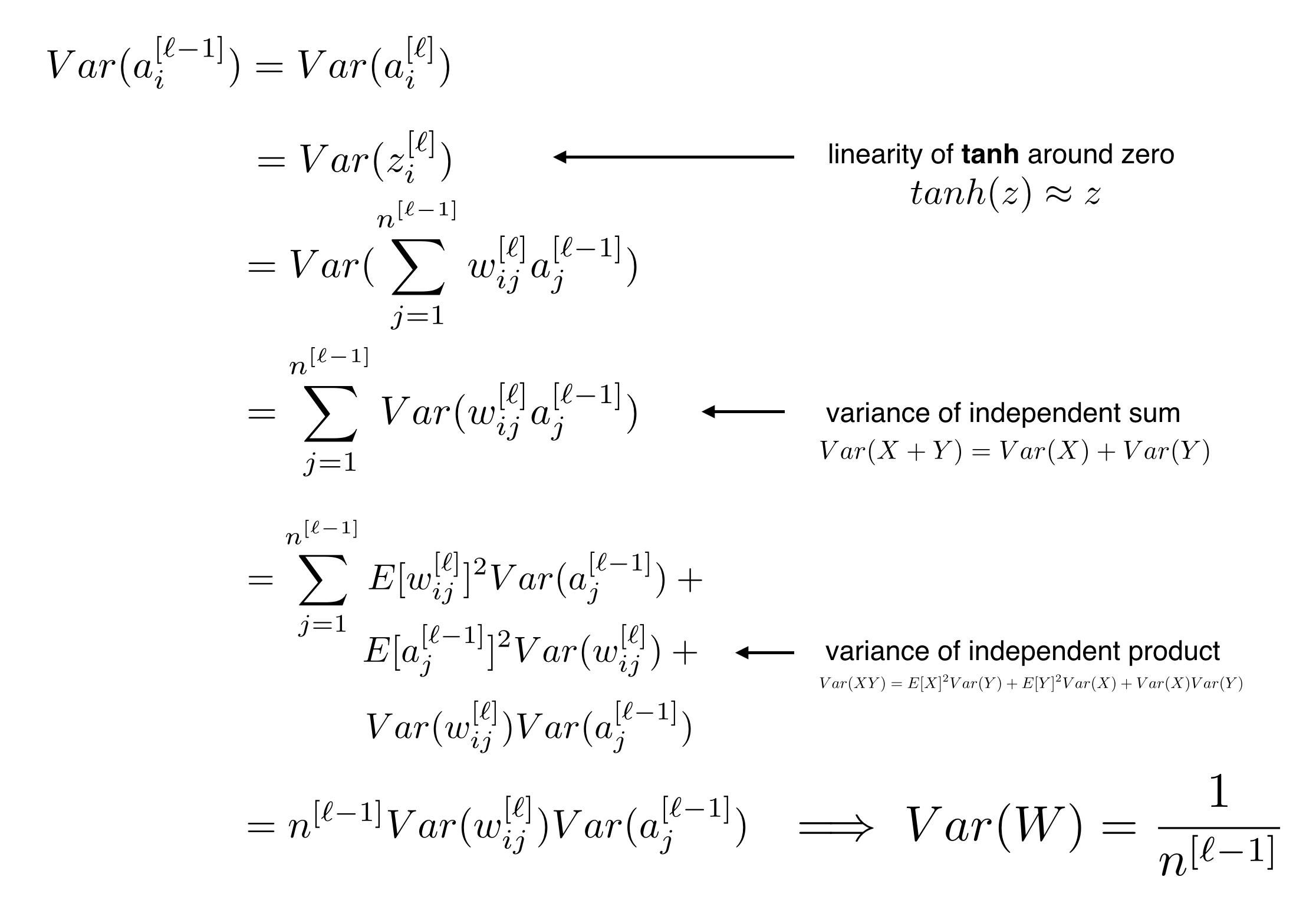
- The goal of Xavier Initialization is to initialize the weights such that the variance of the activations are the same across every layer. This constant variance helps prevent the gradient from exploding or vanishing.
- To help derive our initialization values, we will make the following simplifying assumptions:
- Weights and inputs are centered at zero
- Weights and inputs are independent and identically distributed
- Biases are initialized as zeros
- We use the
tanh()activation function, which is approximately linear for small inputs: \(Var(a^{[l]}) \approx Var(z^{[l]})\)
Derivation: Xavier initialization
- Our full derivation gives us the following initialization rule, which we apply to all weights:
- Xavier initialization is designed to work well with
tanhorsigmoidactivation functions. For ReLU activations, look into He initialization, which follows a very similar derivation.
Further Reading
- Here are some (optional) links you may find interesting for further reading:
- Daniel Kunin’s blog post for a deeper treatment into regularization.
- Chapter 3 of The Elements of Statistical Learning.
Citation
If you found our work useful, please cite it as:
@article{Chadha2020DistilledXavierInit,
  title   = {Xavier Initialization},
  author  = {Chadha, Aman},
  journal = {Distilled AI},
  year    = {2020},
  note    = {\url{https://aman.ai}}
}