Word2Vec
Word2Vec
- Proposed in Efficient Estimation of Word Representations in Vector Space by Mikolov et al. (2013), the Word2Vec algorithm marked a significant advancement in the field of NLP as a notable example of a word embedding technique.
- Word2Vec is renowned for its effectiveness in learning word vectors, which are then used to decode the semantic relationships between words. It utilizes a vector space model to encapsulate words in a manner that captures both semantic and syntactic relationships. This method enables the algorithm to discern similarities and differences between words, as well as to identify analogous relationships, such as the parallel between “Stockholm” and “Sweden” and “Cairo” and “Egypt.”
- Word2Vec’s methodology of representing words as vectors in a semantic and syntactic space has profoundly impacted the field of NLP, offering a robust framework for capturing the intricacies of language and its usage.
Advantages
- Word2Vec introduced a fundamental shift in natural language processing by allowing efficient learning of distributed word representations that capture both semantic and syntactic relationships.
- These embeddings support a wide range of downstream tasks, such as text classification, translation, and recommendation systems, due to their ability to encode meaning in vector space.
- Key advantages include:
- The ability to capture semantic similarity — words appearing in similar contexts have similar vector representations.
- Support for vector arithmetic to reveal analogical relationships (for example, “king - man + woman ≈ queen”).
- Computational efficiency due to simplified training strategies such as negative sampling and hierarchical softmax (covered in detail later).
- A shallow network design, allowing rapid training even on large corpora.
- Generalization across linguistic tasks by representing words in a continuous vector space rather than as discrete symbols.
Theoretical Foundation: Distributional Hypothesis
-
At the heart of Word2Vec lies the distributional hypothesis in linguistics, which states that “words that occur in similar contexts tend to have similar meanings.” Formally, this implies that the meaning of a word \(w\) can be inferred from the statistical distribution of other words that co-occur with it in text.
-
If \(C(w)\) denotes the set of context words appearing around \(w\) within a fixed window, Word2Vec seeks to learn an embedding function \(f: w \mapsto \mathbf{v}_w \in \mathbb{R}^N\) that maximizes the likelihood of observing those context words.
-
Thus, for every word \(w_t\) in the corpus, the training objective is to maximize
\[\frac{1}{T} \sum_{t=1}^{T} \sum_{-c \le j \le c, j \ne 0} \log p(w_{t+j} | w_t)\]- where \(c\) is the context window size and \(T\) is the corpus length.
Representational Power and Semantic Arithmetic
- One of the key insights from Word2Vec is that semantic relationships between words can be captured through linear relationships in vector space. This means that algebraic operations on word vectors can reveal linguistic regularities, such as:
- These relationships emerge naturally because Word2Vec embeds words in such a way that cosine similarity corresponds to semantic relatedness:
- This property allows for analogical reasoning, clustering, and downstream use in a wide range of NLP tasks.
Probabilistic Interpretation
-
From a probabilistic standpoint, Word2Vec models the conditional distribution of context words given a target word (Skip-gram) or a target word given its context (CBOW). The softmax function formalizes this as:
\[p(w_o | w_i) = \frac{\exp(u_{w_o}^T v_{w_i})}{\sum_{w' \in V} \exp(u_{w'}^T v_{w_i})}\]-
where
- \(v_{w_i}\) is the input vector (representing the center or target word),
- \(u_{w_o}\) is the output vector (representing the context word), and
- \(V\) is the vocabulary.
-
-
This formulation defines a differentiable objective that allows embeddings to be learned through backpropagation and stochastic gradient descent.
-
The following figure shows a simplified visualization of the training process using context prediction.
Motivation behind Word2Vec: The Need for Context-based Semantic Understanding
- Traditional approaches to textual representation—such as TF-IDF and BM25—treat words as independent entities and rely on counting-based statistics rather than semantic relationships. While these methods are effective for ranking documents or identifying keyword importance, they fail to represent the contextual and relational meaning that underpins natural language.
- The motivation for Word2Vec arises from the limitations of count-based models that fail to capture semantics. By introducing a predictive, context-driven learning mechanism, Word2Vec constructs a semantic embedding space where contextual relationships between words are preserved. This makes it a foundational technique for subsequent deep learning models such as GloVe, ELMo, and BERT, which further refine contextual understanding at the sentence and discourse level.
Background: Limitations of Frequency-based Representations
-
TF-IDF (Term Frequency–Inverse Document Frequency)
-
This method assigns weights to terms based on how frequently they appear in a document and how rare they are across a corpus.
-
Mathematically, the weight for a term \(t\) in a document \(d\) is given by:
\[\text{TF-IDF}(t, d) = \text{TF}(t, d) \times \log\frac{N}{\text{DF}(t)}\]where \(\text{TF}(t, d)\) is the frequency of term \(t\) in document \(d\), \(\text{DF}(t)\) is the number of documents containing \(t\), and \(N\) is the total number of documents.
-
While TF-IDF captures word importance, it ignores semantic similarity—two words like “doctor” and “physician” are treated as entirely distinct, even though they share similar meanings.
-
-
BM25 (Best Matching 25)
-
BM25 is a probabilistic ranking function often used in information retrieval. It improves upon TF-IDF by introducing parameters to handle term saturation and document length normalization:
\[\text{BM25}(t, d) = \log\left(\frac{N - \text{DF}(t) + 0.5}{\text{DF}(t) + 0.5}\right) \cdot \frac{(k_1 + 1),\text{TF}(t, d)}{k_1!\left[(1 - b) + b\frac{|d|}{\text{avgdl}}\right] + \text{TF}(t, d)}\]where \(k_1\) and \(b\) are tunable parameters, $$ d \(is the document length, and\)\text{avgdl}$$ is the average document length across the corpus. -
BM25 effectively balances term relevance and document length normalization, but it remains a lexical rather than semantic measure. It doesn’t model relationships such as synonymy, antonymy, or analogy.
-
Motivation for Contextual Representations
-
Human language is inherently contextual: the meaning of a word depends on the words surrounding it. For example, the word bank in “river bank” differs from bank in “bank loan.”
- Frequency-based methods cannot distinguish these meanings because they represent bank as a single static token.
- What is required is a context-aware model that learns word meaning from its usage patterns in sentences—capturing semantics not just by frequency, but by co-occurrence structure and distributional behavior.
Word2Vec as a Contextual Solution
- Word2Vec resolves these shortcomings by learning dense, low-dimensional embeddings that encode semantic similarity through co-occurrence patterns.
- Instead of treating each word as an independent unit, Word2Vec models conditional probabilities such as:
- These probabilities are parameterized by neural network weights that correspond to word embeddings.
- Through training, the model positions semantically similar words near each other in the embedding space.
Semantic Vector Space: A Conceptual Leap
- In Word2Vec, each word is represented as a continuous vector \(\mathbf{v}_w \in \mathbb{R}^N\), where semantic similarity corresponds to geometric proximity.
-
This vector representation allows the model to capture linguistic phenomena that statistical models cannot:
- Synonymy: Words like “car” and “automobile” appear near each other.
- Antonymy: Words like “hot” and “cold” occupy positions with structured contrastive relations.
- Analogies: Relationships such as \(\mathbf{v}_{\text{Paris}} - \mathbf{v}_{\text{France}} + \mathbf{v}_{\text{Italy}} \approx \mathbf{v}_{\text{Rome}}\) demonstrate how linear vector operations encode relational meaning.
Comparison with Traditional Models
| Aspect | TF-IDF | BM25 | Word2Vec |
|---|---|---|---|
| Representation | Sparse, count-based | Sparse, probabilistic | Dense, continuous |
| Captures context | No | No | Yes |
| Semantic similarity | Not modeled | Not modeled | Explicitly modeled |
| Handles polysemy | No | No | Partially (through contextual learning) |
| Learning mechanism | Frequency-based | Probabilistic ranking | Neural prediction |
Why Context Matters: Intuitive Illustration
- Imagine reading the sentence:
“The bat flew across the cave.”
- and another:
“He swung the bat at the ball.”
- In traditional models, the token “bat” is identical in both contexts.
- However, Word2Vec distinguishes them by how “bat” co-occurs with words like flew, cave, swung, and ball. The embeddings for these contexts push the representation of bat toward two distinct regions of the semantic space—one near animals, the other near sports equipment.
Core Idea
- Word2Vec represents a transformative shift in natural language understanding by learning word meanings through prediction tasks rather than through counting word co-occurrences.
- At its core, the algorithm employs a shallow neural network trained on a large corpus to predict contextual relationships between words, producing dense, meaningful vector representations that encode both syntactic and semantic regularities.
- The core idea behind Word2Vec is to transform linguistic co-occurrence information into a geometric form that captures word meaning through spatial relationships. It does this not by memorizing frequencies, but by predicting contexts, allowing the embedding space to inherently encode semantic similarity, analogy, and syntactic relationships in a mathematically continuous manner.
Predictive Nature of Word2Vec
-
Unlike earlier statistical methods that rely on co-occurrence counts (e.g., Latent Semantic Analysis), Word2Vec learns embeddings by solving a prediction problem:
- Given a target word, predict its context words (Skip-gram).
- Given a set of context words, predict the target word (CBOW).
-
This approach stems from the distributional hypothesis, operationalized via probabilistic modeling.
-
Formally, for a corpus with words \(w_1, w_2, \dots, w_T\), and context window size \(c\), the model maximizes the following average log probability:
- This objective encourages the model to learn embeddings \(\mathbf{v}_{w_t}\) and \(\mathbf{u}_{w_{t+j}}\) such that similar words (those that appear in similar contexts) have similar vector representations.
Word Vectors and Semantic Encoding
-
Each word \(w\) in the vocabulary is associated with two vectors:
- Input vector \(\mathbf{v}_w\): representing the word when it is the center (target) word.
- Output vector \(\mathbf{u}_w\): representing the word when it appears in the context.
-
These vectors are columns in the weight matrices:
- \(\mathbf{W} \in \mathbb{R}^{V \times N}\) (input-to-hidden layer)
- \(\mathbf{W}' \in \mathbb{R}^{N \times V}\) (hidden-to-output layer)
-
Thus, the total parameters of the model are \(\theta = {\mathbf{W}, \mathbf{W}'}\), and for any word \(w_i\) and context word \(c\):
\[p(w_i | c) = \frac{\exp(\mathbf{u}_{w_i}^T \mathbf{v}_c)}{\sum*{w'=1}^{V} \exp(\mathbf{u}_{w'}^T \mathbf{v}_c)}\] -
This softmax-based conditional probability is the foundation for learning embeddings that maximize the likelihood of true word–context pairs.
Vector Arithmetic and Semantic Regularities
- One of Word2Vec’s most striking properties is its ability to encode linguistic regularities as linear relationships in vector space.
- For example:
- Such arithmetic operations are possible because the training objective aligns words based on shared contextual usage.
- Consequently, the cosine similarity between two word vectors reflects their semantic closeness:
Network Architecture and Operation
-
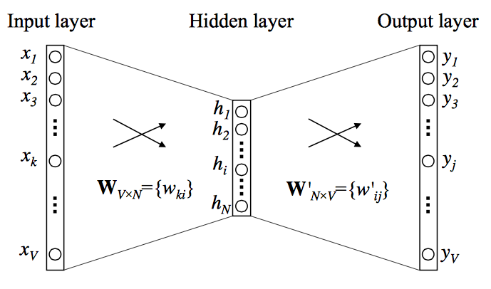
The following figure shows the overall neural network structure underlying Word2Vec, consisting of:
- Input layer — one-hot encoded representation of a word.
- Hidden layer — the embedding layer, of dimensionality \(N\), where words are projected into a dense vector space.
- Output layer — a softmax over the vocabulary predicting either the target (CBOW) or context (Skip-gram).
-
The hidden layer’s weights become the learned word embeddings.
-
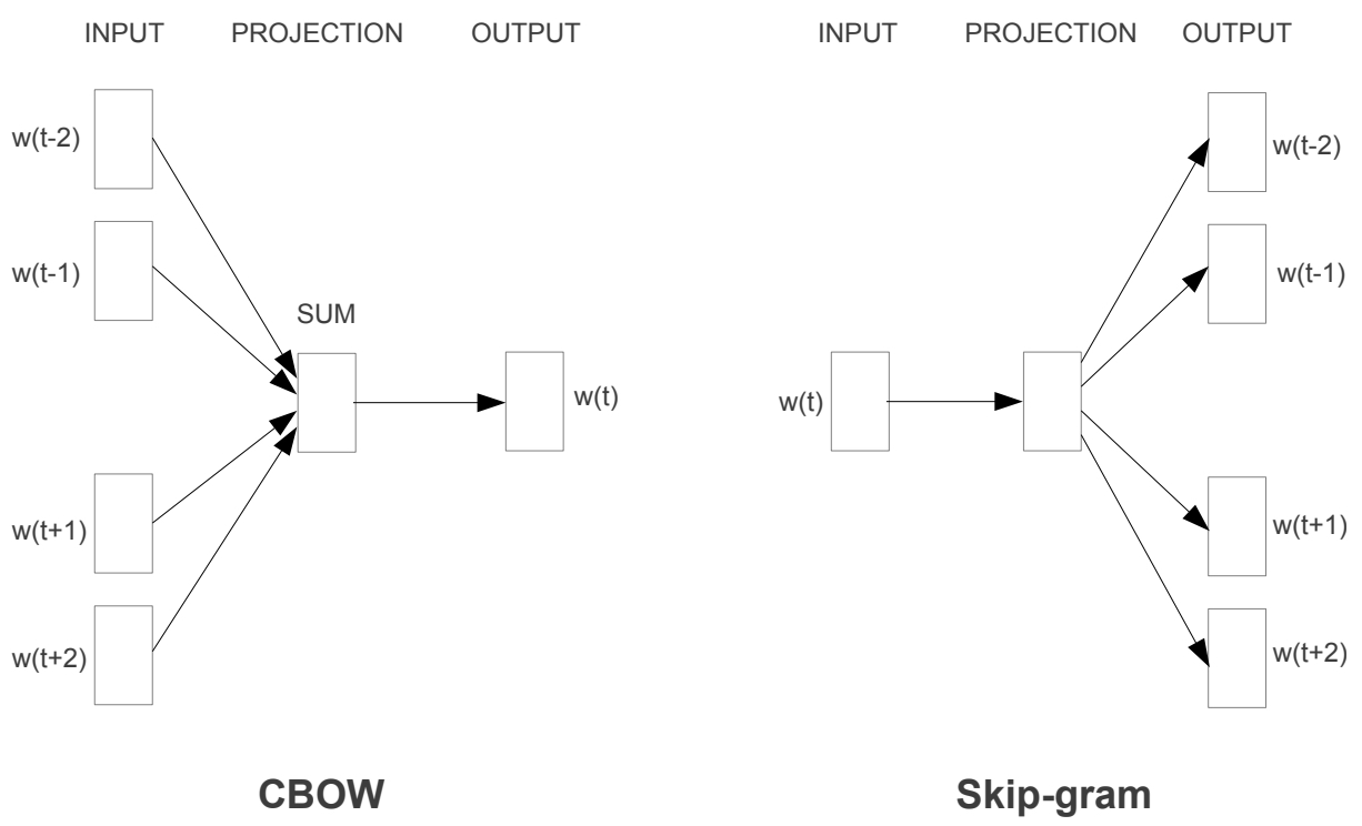
The following figure shows a visualization of this architecture and the two modeling directions — CBOW and Skip-gram.
Interpretability of the Embedding Space
-
Through iterative training across billions of word pairs, the model learns embeddings such that:
- Words that appear in similar contexts have similar directions in the vector space.
- Analogous relationships are captured through vector offsets.
- Syntactic categories (e.g., plurals, verb tenses) and semantic groupings (e.g., cities, countries) naturally emerge as clusters.
-
For instance, after training, the vectors for [“Paris”, “London”, “Berlin”] form a subspace distinct from [“France”, “UK”, “Germany”], yet maintain parallel structure, enabling analogical reasoning such as:
Word2Vec Architectures
- Word2Vec offers two distinct neural architectures for learning word embeddings:
- Continuous Bag-of-Words (CBOW)
- Continuous Skip-gram (Skip-gram)
- Both are trained on the same corpus using similar mechanisms but differ in the direction of prediction — that is, whether the model predicts the center word from its context words or the context words from the center word. Both CBOW and Skip-gram learn embeddings that reflect word meaning through context prediction.
- CBOW excels in efficiency and stability for frequent words, while Skip-gram provides richer embeddings for rare words.
- Together, they form the foundation of Word2Vec’s success — enabling scalable and semantically powerful word representations.
Continuous Bag-of-Words (CBOW)
-
Concept:
- The CBOW model predicts the target (center) word based on the words surrounding it.
- Given a window of context words \(C_t = {w_{t-c}, \ldots, w_{t-1}, w_{t+1}, \ldots, w_{t+c}}\), the goal is to maximize:
- This makes CBOW a context-to-word model — the inverse of Skip-gram.
-
Architecture:
- The following figure shows the CBOW model, where multiple context word one-hot vectors are fed into a shared embedding matrix, averaged, and used to predict the central target word.
- Mathematically, the average of the context word vectors is computed as:
- The probability of predicting the target word \(w_t\) given this averaged context is then defined using the softmax function:
-
Learning Objective:
- The training objective maximizes the log-likelihood across the corpus:
- Gradients are propagated to update both input (\(\mathbf{v}_w\)) and output (\(\mathbf{u}_w\)) embeddings via stochastic gradient descent.
-
Parameterization:
-
For a given word index \(k\) in vocabulary \(V\), the referenced word is represented as:
- Input vector \(\mathbf{v}_w = \mathbf{W}_{(k, .)}\)
- Output vector \(\mathbf{u}_w = \mathbf{W}'*{(., k)}\)
-
The hidden layer has \(N\) neurons, and the model learns weight matrices \(\mathbf{W} \in \mathbb{R}^{V \times N}\) and \(\mathbf{W}' \in \mathbb{R}^{N \times V}\).
-
-
Overall Formula:
\[p(w_i | c) = y_i = \frac{e^{u_i}}{\sum_{i=1}^V e^{u_i}}, \quad \text{where } u_i = \mathbf{u}_{w_i}^T \mathbf{v}_c\]
Continuous Skip-gram (SG)
-
Concept:
- The Skip-gram model reverses CBOW’s direction:
-
Instead of predicting the target from the context, it predicts context words from the center word.
-
Formally, the Skip-gram objective is to maximize the likelihood of context words given the center word \(w_t\):
\[\mathcal{L}_{SG} = \frac{1}{T} \sum*{t=1}^{T} \sum_{-c \le j \le c, j \ne 0} \log p(w_{t+j} | w_t)\]- where \(c\) is the context window size.
-
Architecture:
- The following figure shows both the CBOW and Skip-gram models side-by-side.
- In Skip-gram, the input is a single one-hot word vector, and the model predicts multiple context words as outputs through a shared embedding space.
-
Softmax Prediction:
- Each pair \((w_t, w_{t+j})\) is modeled as:
-
Learning Objective:
- The Skip-gram model maximizes the overall log-likelihood:
-
Here, every occurrence of a word generates multiple (target → context) prediction pairs, which makes training computationally heavier but more expressive — particularly for rare words.
Comparison: CBOW vs Skip-gram
| Aspect | CBOW | Skip-gram |
|---|---|---|
| Prediction Direction | Context → Target | Target → Context |
| Input | Multiple context words | Single target word |
| Output | One target word | Multiple context words |
| Training Speed | Faster | Slower |
| Works Best For | Frequent words | Rare words |
| Robustness | Smoother embeddings | More detailed embeddings |
| Objective Function | \(\log p(w_t \mid C_t)\) | \(\sum_{-c \le j \le c, j \ne 0} \log p(w_{t+j} \mid w_t)\) |
Why Skip-gram Handles Rare Words Better
- Skip-gram updates the embeddings of the center word for each of its context words.
- If a rare word appears even once, it still generates multiple (target, context) pairs, each leading to gradient updates for that word.
-
By contrast, CBOW uses rare words as targets — meaning they are predicted less often and receive fewer updates, leading to less precise embeddings.
- Example:
- In the sentence “The iguana basked on the rock”, the rare word “iguana” generates pairs such as (iguana → the), (iguana → basked), (iguana → on), (iguana → rock), thus updating its embedding multiple times in Skip-gram, whereas CBOW would update it only once.
Which Model to Use When
-
Use CBOW when:
- The dataset is large and contains many frequent words.
- You require fast training and smoother embeddings.
- The task emphasizes semantic similarity among common words (e.g., topic clustering, document similarity).
- Example: Training on Wikipedia or Common Crawl for general-purpose embeddings.
-
Use Skip-gram when:
- The dataset is smaller or contains many rare and domain-specific words.
- Skip-gram performs better in such cases because it creates multiple training pairs for each occurrence of a rare word, giving it more opportunities to learn meaningful relationships from limited data.
- You want to capture fine-grained syntactic or semantic nuances.
- The focus is on representation quality rather than speed.
- Example: Training embeddings for biomedical text, legal documents, or historical corpora.
-
Hybrid Strategy:
- Some implementations begin with CBOW pretraining and fine-tune with Skip-gram for precision.
- For multilingual or low-resource settings, Skip-gram tends to outperform due to its capacity to learn detailed contextual cues from fewer examples.
Training and Optimization
- The training of Word2Vec centers on optimizing word embeddings so that they accurately predict contextual relationships between words. Each word in the vocabulary is assigned two learnable vectors: one for when it acts as a target (input) and another for when it acts as a context (output) word. These vectors are iteratively updated during training to minimize a prediction loss.
Objective Function
-
The central objective of Word2Vec is to maximize the probability of correctly predicting context words given a target word (in Skip-gram) or the target word given its context (in CBOW).
-
Formally, for Skip-gram, this objective is expressed as:
- and for CBOW:
- Both of these involve computing probabilities using the softmax function, defined as:
-
where:
- \(v_{w_i}\) is the input vector of the target word,
- \(u_{w_o}\) is the output vector of the context word,
- \(V\) is the vocabulary size.
Why the Full Softmax Is Computationally Expensive
- The denominator of the softmax requires summing over all words in the vocabulary.
-
For large corpora (where $$ V $$ can exceed millions), this operation must be repeated for every training pair — making it computationally prohibitive. - To address this, Mikolov et al. introduced two key approximation methods: Negative Sampling and Hierarchical Softmax.
Negative Sampling
- Concept:
- Negative Sampling reframes the prediction task as a binary classification problem.
- For each observed (target, context) pair, the model learns to distinguish it from \(K\) randomly sampled “negative” pairs (words that did not co-occur).
- Loss Function:
- For a single (target, context) pair ((w_i, w_o)), the loss function becomes:
-
where:
- \(\sigma(x) = \frac{1}{1 + e^{-x}}\) is the sigmoid function,
- \(w_o\) is a true context word,
- \(w_k\) are \(K\) negative samples drawn from a noise distribution (typically proportional to word frequency raised to the ¾ power).
-
This approach dramatically reduces computation because only a small number of words (positive + negatives) are updated per training step instead of the entire vocabulary.
-
Intuition:
- Positive pairs push their embeddings closer together (increase similarity).
-
Negative pairs push their embeddings apart (decrease similarity).
- This yields embeddings where semantically related words occupy nearby regions in vector space.
Hierarchical Softmax
- Concept:
- Hierarchical Softmax replaces the flat softmax layer with a binary tree (often a Huffman tree).
- Each word in the vocabulary becomes a leaf node, and the probability of a word is computed as the product of probabilities along the path from the root to that leaf.
- Loss Function:
- If a word \(w\) follows a path defined by internal nodes \(n_1, n_2, \dots, n_L\), with binary decisions \(d_i \in {0, 1}\) at each node, the probability of \(w\) is:
-
This reduces computational complexity from $$O( V )\(to\)O(\log V )$$, making it efficient for very large vocabularies.
Optimization Process
- Both CBOW and Skip-gram are trained using stochastic gradient descent (SGD) or variants such as Adam or Adagrad.
-
At each step:
- The model samples a target word and its context (or vice versa).
- Computes the predicted probability using either softmax, hierarchical softmax, or negative sampling.
- Updates the corresponding embeddings using gradients derived from the loss.
-
Gradients are propagated as follows:
- Positive pairs increase the dot product \(u_{w_o}^T v_{w_i}\).
- Negative pairs decrease it.
- This iterative process converges when embeddings stabilize and begin representing consistent contextual meaning.
Training Visualization
- The following figure shows a conceptual visualization of the training process, where the model adjusts embeddings such that words appearing in similar contexts are geometrically closer in the vector space.
Embedding and Semantic Relationships
-
Word2Vec’s training process produces a set of word vectors (embeddings) that encode semantic and syntactic information in a continuous, semantically meaningful geometric space.
- Proximity represents similarity of meaning.
- Direction represents relational structure.
- Linear operations capture analogies and transformations.
- This property makes Word2Vec a cornerstone in modern NLP — providing not only compact word representations but also interpretable relationships that reflect the way humans understand language.
- These embeddings are powerful because they convert discrete linguistic units (words) into numerical representations that reflect meaning, contextual similarity, and linguistic regularities.
From Co-occurrence to Geometry
-
During training, Word2Vec positions each word vector \(\mathbf{v}_w \in \mathbb{R}^N\) such that words occurring in similar contexts are close to each other in the embedding space.
-
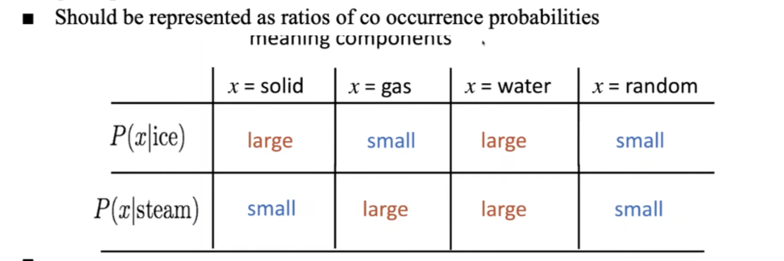
Mathematically, if two words \(w_i\) and \(w_j\) share similar context distributions, their conditional probabilities $$p(C w_i)\(and\)p(C w_j)$$ are alike, leading to embeddings with high cosine similarity:
- This means that words like dog and cat, which appear in similar linguistic environments (e.g., near words like pet, animal, food), will have vectors oriented in similar directions.
Linear Relationships and Analogy
- One of the most celebrated properties of Word2Vec embeddings is their ability to capture analogical relationships using simple linear algebra.
-
These relationships emerge naturally from the model’s predictive training objective, which enforces consistent geometric offsets between semantically related words.
- For instance:
- This implies that the relationship between “man” and “woman” is encoded as a directional vector offset in the space, and the same offset applies to other analogous pairs like:
Clustering and Semantic Neighborhoods
-
When visualized (e.g., using t-SNE or PCA), Word2Vec embeddings form clusters that group together semantically or syntactically similar words.
- Semantic clusters: Words such as dog, cat, horse, cow cluster under the broader concept of animals.
- Syntactic clusters: Words like running, swimming, jumping cluster based on grammatical function (verbs in gerund form).
-
In this space, semantic similarity corresponds to spatial proximity, and semantic relations correspond to vector directions.
Interpreting the Embedding Space
- The embedding space captures multiple types of relationships:
| Relationship Type | Example | Geometric Interpretation |
|---|---|---|
| Synonymy | happy ↔ joyful | Small cosine distance |
| Antonymy | good ↔ bad | Large angle, opposite directions |
| Hierarchical | car ↔ vehicle | “Parent–child” proximity |
| Analogical | king – man + woman ≈ queen | Consistent vector offset |
- This geometric consistency arises because the dot product \(u_{w_o}^T v_{w_i}\) — central to Word2Vec’s loss function — forces the space to preserve relational proportionality among co-occurring words.
Example: Semantic Continuity
-
To illustrate, consider these relationships in trained embeddings:
- \[\mathbf{v}_{\text{France}} - \mathbf{v}_{\text{Paris}} \approx \mathbf{v}_{\text{Italy}} - \mathbf{v}_{\text{Rome}}\]
- \[\mathbf{v}_{\text{walking}} - \mathbf{v}_{\text{walk}} \approx \mathbf{v}_{\text{running}} - \mathbf{v}_{\text{run}}\]
-
Both examples demonstrate that semantic and syntactic transformations (capital–country or verb–tense) are encoded as parallel vectors in the embedding space.
Visualization of Analogical Relationships
- The following figure shows how vector arithmetic captures analogical reasoning, where the learned embeddings reveal semantic structure and relational symmetry.
Distinction from Traditional Models
- Word2Vec represents a fundamental paradigm shift from earlier count-based and probabilistic language models.
-
Traditional methods typically relied on explicit frequency counts or co-occurrence matrices, while Word2Vec learns distributed representations that are continuous, dense, and semantically meaningful. Word2Vec diverges from traditional models by:
- Moving from counting to predicting, thus learning generalized patterns.
- Embedding words in a continuous space, allowing geometric interpretation.
- Capturing semantics and syntax simultaneously, through context-based optimization.
- These distinctions made Word2Vec the first widely adopted neural representation model, bridging the gap between symbolic and distributed semantics in NLP.
Traditional Count-based Models
- Before neural embeddings, most language representations were derived from word frequency statistics.
-
Co-occurrence Matrices:
-
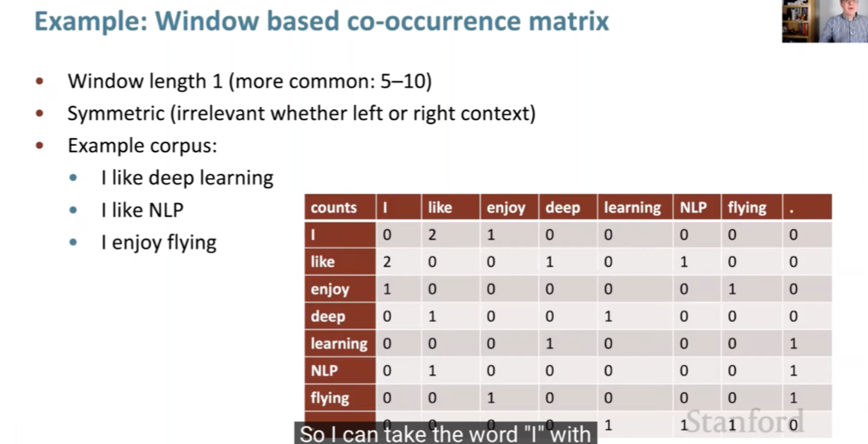
These models record how often each word appears with every other word in a fixed context window.
-
\[M_{ij} = \text{count}(w_i, w_j)\]The resulting matrix $$M \in \mathbb{R}^{ V \times V }$$ has entries: - where \(\text{count}(w_i, w_j)\) denotes how many times word \(w_j\) occurs near word \(w_i\).
- High-dimensional and extremely sparse, these matrices often undergo dimensionality reduction (e.g., SVD or PCA) to extract latent features.
-
-
TF-IDF Representations:
-
Assign weights to words based on their document-specific frequency and global rarity:
\[\text{TF-IDF}(t, d) = \text{TF}(t, d) \times \log\frac{N}{\text{DF}(t)}\] -
Useful for document retrieval, but insensitive to word order or semantic relationships.
-
-
Topic Models (e.g., LDA):
- Represent documents as mixtures of latent “topics” inferred through probabilistic modeling.
- While they uncover thematic structure, they don’t provide fine-grained word-level semantics or geometric relationships.
Predictive vs. Count-based Philosophy
-
The essential distinction is predictive learning versus statistical counting:
Feature Count-based Models (e.g., TF-IDF, LSA) Predictive Models (Word2Vec) Representation Sparse, frequency-based Dense, distributed Learning Objective Approximate co-occurrence statistics Predict neighboring words Captures Context Implicitly via counts Explicitly via prediction Semantic Structure Limited, global Rich, local and continuous Computational Method Matrix decomposition Neural optimization Output Dimensionality Fixed by vocabulary Tunable (e.g., 100–300 dimensions) -
Key insight: Count-based models memorize co-occurrence patterns, while Word2Vec learns to predict them. This predictive training enables the embeddings to generalize beyond exact word occurrences — capturing unseen but semantically related patterns.
Connection to Matrix Factorization
- Although Word2Vec is a neural model, it is mathematically related to implicit matrix factorization.
- As shown in later research (Levy & Goldberg, 2014), Skip-gram with Negative Sampling (SGNS) implicitly factorizes a shifted Pointwise Mutual Information (PMI) matrix:
-
SGNS effectively learns vectors \(\mathbf{v}_w, \mathbf{u}_c\) such that:
\[\mathbf{v}_w^T \mathbf{u}_c \approx \text{PMI}(w, c) - \log k\]- where \(k\) is the number of negative samples.
-
Thus, Word2Vec can be seen as a learned, smoothed, and low-dimensional version of PMI-based co-occurrence models, optimized through stochastic gradient descent instead of explicit decomposition.
Contextual Encoding and Generalization
-
Traditional models treat each word as an independent symbol; the model cannot infer that doctor and physician are semantically related. In contrast, Word2Vec represents both words as nearby vectors because they occur in similar contexts, such as hospital, patient, or medicine.
-
This contextual generalization enables tasks like:
- Synonym detection (high cosine similarity)
- Analogy reasoning (vector offsets)
- Clustering and semantic grouping
-
These capabilities were not achievable with bag-of-words or count-based models, which lacked a mechanism to encode relational meaning.
Computational Perspective
-
Word2Vec also introduced major computational improvements:
- Scalability: The use of negative sampling and hierarchical softmax allows training on billions of words efficiently.
- Memory Efficiency: Each word is represented by compact \(N\)-dimensional vectors (e.g., 300 dimensions) instead of huge sparse vectors.
- Incremental Learning: Embeddings can be updated online, unlike matrix factorization, which must process entire corpora at once.
Semantic Nature of Word2Vec Embeddings
-
Word2Vec embeddings are semantic in nature because they encode meaningful relationships between words based on their distributional context. Rooted in the distributional hypothesis — the idea that “words appearing in similar contexts tend to have similar meanings” — Word2Vec learns to embed words in a vector space by predicting their surrounding context. This training objective forces words with similar usage to acquire similar vector representations.
-
As a result, the geometry of the embedding space captures semantic similarity through distance, and analogical relationships through direction. These geometric properties enable a wide range of linguistic tasks, such as clustering similar words, solving analogies, and performing semantic reasoning, all via simple vector operations.
-
Together, these capabilities make Word2Vec one of the earliest and most intuitive examples of how neural networks can internalize and represent linguistic meaning through learned representations.
How Semantic Meaning Emerges
- During training, each word \(w_t\) is optimized such that its embedding \(\mathbf{v}_{w_t}\) maximizes the likelihood of co-occurring context words \({w*{t+j}}\).
-
As a result, words that occur in similar environments receive similar gradient updates, causing their vectors to align in space.
- Formally, if two words \(w_a\) and \(w_b\) share overlapping context distributions:
- then their embeddings converge to similar directions:
- This geometric proximity encodes semantic relatedness — the closer the vectors, the more semantically similar the words.
CBOW and Skip-gram as Semantic Learners
-
CBOW Model:
- Predicts a target word given its context.
- Learns smoother embeddings by averaging contextual information, leading to stable semantic representations for frequent words.
- Example: Predicting “mat” from the context “The cat sat on the ___” helps reinforce relationships between cat, sat, and mat.
-
Skip-gram Model:
- Predicts multiple context words from a single target.
- Captures more fine-grained semantic details, especially for rare words.
- Example: Given “cat”, Skip-gram learns to predict “the”, “sat”, “on”, and “mat”, enriching cat’s embedding through diverse contextual associations.
- Together, these architectures operationalize the distributional hypothesis through context-based prediction, transforming textual co-occurrence patterns into structured vector relationships.
Types of Semantic Relationships Captured
- Similarity
- Words with related meanings are embedded close together. For * instance, dog, cat, and puppy form a tight cluster in the embedding space due to shared usage contexts.
- Analogy
- Linear relationships in vector space reflect semantic analogies such as:
- This pattern generalizes across many relationships (capital–country, gender, verb tense, etc.), e.g.:
- Clustering
-
Semantic similarity also manifests as clusters within the high-dimensional space:
- Animals*: {dog, cat, horse, cow}
- Countries*: {France, Germany, Italy, Spain}
- Emotions*: {happy, joyful, cheerful, glad}
-
Clustering results from the model’s ability to map semantically related words to nearby regions in the embedding space.
-
Geometric and Semantic Interpretations
- Each semantic relationship has a geometric counterpart:
| Relationship Type | Example | Geometric Interpretation |
|---|---|---|
| Synonymy | car ↔ automobile | Small cosine distance |
| Analogy | man → woman :: king → queen | Parallel vector offset |
| Hypernymy | dog → animal | Direction along hierarchical axis |
| Antonymy | good ↔ bad | Large angular separation |
| Morphology | walk → walking | Consistent offset along tense dimension |
- This shows that semantics are encoded directionally and proportionally in the embedding space — a key reason Word2Vec embeddings are interpretable through vector arithmetic.
Analogy through Vector Arithmetic
- Word2Vec’s training objective aligns embedding directions in such a way that analogical reasoning emerges naturally.
- If a relationship between two words is represented as a consistent vector offset, then:
- For example:
- This reveals a kind of semantic isomorphism — a structural preservation of relationships across conceptual domains.
The Following Figure Shows Semantic Analogies
- The following figure shows how semantic and syntactic relationships (e.g., gender, verb tense, geography) appear as consistent linear transformations in the vector space.
Key Limitations and Advances in Word2Vec and Word Embeddings
-
Word2Vec remains one of the most influential frameworks in the evolution of natural language processing (NLP), revolutionizing the field with its ability to encode meaning geometrically. By representing words as continuous vectors in a semantic space, it enabled machines to understand words not merely as symbolic tokens, but as entities with inherent relationships and structure.
-
However, despite its groundbreaking impact, Word2Vec’s design introduces several inherent limitations that eventually spurred the development of more advanced contextualized embedding models. These limitations stem primarily from its static and context-independent nature—each word is assigned a single vector, regardless of its varying meanings in different contexts. Additionally, Word2Vec’s approach to processing context and dealing with data sparsity posed further challenges in capturing nuanced language use.
-
To address these shortcomings, newer models emerged that not only capture the general meaning of words but also adapt dynamically to their context within a sentence or document. These contextualized embeddings now form the foundation of modern NLP, offering a far more flexible and precise understanding of language.
Static, Non-Contextualized Nature
-
Single Vector per Word:
- In Word2Vec, each word type is represented by one fixed embedding, regardless of the sentence or context in which it appears.
- For instance, the word “bank” is assigned a single vector whether it refers to a financial institution or the side of a river.
-
As a result, multiple senses of a word (polysemy) are collapsed into a single point in the embedding space.
- Mathematically, for all occurrences of a word \(w\), Word2Vec assigns one embedding \(\mathbf{v}_w \in \mathbb{R}^N\), such that:
independent of its local context.
- This static representation means that semantic disambiguation is impossible within the model itself.
-
Combination of Contexts:
- Because all usages of a word are averaged during training, the resulting embedding represents an aggregate of multiple meanings.
- For example, “apple” in “Apple released a new iPhone” (corporate sense) and “I ate an apple” (fruit sense) are both used to update the same embedding vector.
- The consequence is a semantic compromise — embeddings become blurry averages of distinct meanings.
-
Lack of Contextual Adaptation:
- Word2Vec’s fixed-size context window only captures local co-occurrence statistics, not long-range dependencies or sentence-level structure.
-
Thus, the model cannot adapt a word’s meaning dynamically based on its syntactic role or broader discourse context.
- Example:
- “She read a book.”
- “He will book a flight.” Word2Vec assigns nearly identical vectors to “book” in both cases, even though one is a noun and the other a verb.
Training Process and Computational Considerations
-
Training Adjustments:
- Throughout training, Word2Vec adjusts embeddings through stochastic gradient descent to improve co-occurrence prediction accuracy.
- However, these updates are purely statistical — not semantic — meaning the model refines embeddings globally rather than creating distinct sense representations.
-
Computational Demands:
- Although optimized via negative sampling, training large vocabularies (millions of words) still requires significant computational resources and memory.
- Furthermore, retraining or updating embeddings for new corpora often demands complete reinitialization, since Word2Vec lacks an efficient fine-tuning mechanism.
Handling of Special Cases
-
Phrase and Idiom Representation:
- Word2Vec struggles with multi-word expressions or idioms whose meanings are non-compositional.
- For instance, “hot potato” or “New York Times” cannot be represented by simply averaging the vectors of their component words.
- As proposed by Mikolov et al. (2013), one partial solution was to treat frequent phrases as single tokens using statistical co-occurrence detection.
-
Out-of-Vocabulary (OOV) Words:
- Word2Vec cannot generate embeddings for words not seen during training.
- This limitation is particularly problematic for morphologically rich or non-segmented languages.
- Later models such as FastText addressed this by representing words as compositions of character n-grams, allowing generalization to unseen forms.
Global Vector Representation Limitations
-
Uniform Representation Across Contexts:
- Word2Vec, like GloVe, produces a global vector for each word.
- This uniformity neglects that a word’s meaning shifts with context.
- For example, the embeddings for “light” cannot distinguish between “light weight” and “light bulb.”
-
Sentiment Polarity and Context Sensitivity:
- Because Word2Vec relies on unsupervised co-occurrence statistics, it can place antonyms such as “good” and “bad” near each other if they occur in similar syntactic positions.
- This leads to issues in sentiment analysis tasks, where distinguishing polarity is essential.
- Tang et al. (2014) proposed Sentiment-Specific Word Embeddings (SSWE), which integrate polarity supervision into the loss function to separate words by sentiment.
Resulting Embedding Compromises
- The outcome of these constraints is that Word2Vec embeddings, though semantically meaningful on average, are context-agnostic and therefore less precise for downstream tasks requiring nuanced interpretation. This trade-off — efficiency and generality versus contextual precision — defined the next phase of NLP research.
Advances Beyond Word2Vec
-
To overcome these challenges, newer models introduced contextualized embeddings, where a word’s representation dynamically changes depending on its sentence-level context.
-
GloVe (Global Vectors for Word Representation):
- Combines local co-occurrence prediction (like Word2Vec) with global matrix factorization.
- Encodes both semantic relationships and global corpus statistics.
-
FastText:
- Represents words as the sum of subword (character n-gram) embeddings, enabling generalization to unseen or rare words.
- Particularly effective for morphologically rich languages.
-
ELMo (Embeddings from Language Models):
- Generates context-dependent embeddings using a bidirectional LSTM language model.
- A word’s vector \(\mathbf{v}_{w, \text{context}}\) depends on its surrounding sentence, allowing dynamic sense representation.
-
BERT (Bidirectional Encoder Representations from Transformers):
- Leverages the Transformer architecture to model bidirectional context simultaneously.
- Each occurrence of a word is encoded uniquely as a function of the entire sequence, capturing fine-grained semantics, syntax, and disambiguation.
-
Formally, embeddings are contextualized as:
\[\mathbf{v}_{w_i} = f(w_i, w*{1:T})\]- where \(f\) is a deep transformer function conditioned on the entire input sentence.
-
Computational Challenges and Approximations
- Although contextual models supersede Word2Vec conceptually, its innovations in efficient optimization remain foundational.
-
Word2Vec introduced practical strategies that allowed large-scale training long before transformer-based systems existed.
- Softmax Approximation Challenge
- Computing the denominator in the softmax function:
- required summing over the entire vocabulary, which is computationally infeasible for large corpora.
- Negative Sampling Solution
- Word2Vec replaced the full softmax with negative sampling, reframing prediction as a binary classification task:
- Here, positive word pairs are pulled closer in vector space, and random negative pairs are pushed apart — allowing efficient updates with only a few sampled words per step.
- Hierarchical Softmax
-
An alternate efficiency method that organizes the vocabulary as a Huffman tree, reducing computational complexity from $$O( V )\(to\)O(\log V )$$.
-
- Softmax Approximation Challenge
- These innovations enabled Word2Vec to scale to billions of tokens — laying the groundwork for subsequent neural representation learning.
Evolutionary Summary
| Generation | Example Models | Key Advancement |
|---|---|---|
| Count-based | TF-IDF, LSA | Frequency and co-occurrence statistics |
| Predictive Static | Word2Vec, GloVe, FastText | Distributed representations of word meaning |
| Contextualized | ELMo, BERT, GPT | Dynamic embeddings conditioned on full sentence context |