Token Sampling Methods
- Overview
- Background
- Temperature
- Greedy Decoding
- Exhaustive Search Decoding
- Beam Search
- Constrained Beam Search
- Top-\(k\) Sampling
- Top-\(p\) (Nucleus Sampling)
- Greedy vs. Top-\(k\) and Top-\(p\)
- min-\(p\) Sampling
- Comparative Analysis
- Related: Sampling from a Probability Distribution
- References
Overview
-
Large Language Models (LLMs) are a class of neural network models designed to generate and understand human language by predicting the next token in a sequence given prior context. Tokens are discrete units of text; depending on the tokenizer they may represent individual characters, subwords, or whole words. Transformer-based LLMs scale to billions or trillions of parameters and are trained using self-supervised learning, typically minimizing the negative log-likelihood of predicting the next token across large corpora of text. The advent of the Transformer architecture by the Attention Is All You Need by Vaswani et al. (2017), enabled highly parallelizable training and laid the foundation for modern LLMs.
-
Subsequent models such as the GPT series (e.g., Improving Language Understanding by Generative Pre-Training by Radford et al. (2018); Language Models Are Few-Shot Learners by Brown et al. (2020)) adopt an autoregressive decoding objective in which the model estimates the probability distribution over the next token conditioned on all previous ones. This can be written as:
\[p(x_{1}, x_{2}, \ldots, x_{T}) = \prod_{t=1}^{T} p(x_{t} \mid x_{<t})\]- where \(x_{t}\) is the token at position \(t\) and \(x_{<t}\) denotes all preceding tokens in the sequence.
-
Training such models on massive corpora yields strong performance on a variety of downstream natural language processing tasks, as surveyed comprehensively in “Large Language Models: A Survey” by Minaee et al. (2024) and A Comprehensive Overview of Large Language Models by Naveed (2023), which collectively summarize architecture, training methods, and evaluation benchmarks across prominent LLM families (e.g., GPT, Llama, PaLM).
-
When generating text (inference time), an LLM produces a probability distribution over all tokens in its vocabulary at each step. The decoding strategy determines how that distribution is used to select the next token. Token selection techniques vary from deterministic approaches (e.g., greedy decoding) to stochastic sampling (e.g., top-\(k\), top-\(p\)/nucleus sampling), and hybrid methods like beam search that balance breadth and probability of hypotheses. The choice of decoding strategy significantly influences the fluency, diversity, and quality of generated text, which has been empirically established in studies such as The Curious Case of Neural Text Degeneration by Holtzman et al. (2019), where the authors show how sampling methods can avoid degenerate text patterns produced by naive maximization decoding.
-
In this primer, we will explore the decoding strategies used in LLMs along with related concepts such as temperature, greedy decoding, beam search, top-\(k\), top-\(p\) (nucleus sampling), and emerging approaches like min-\(p\) sampling, illustrating both mathematical foundations and practical behavior differences.
Background
Autoregressive Decoding
-
Modern large language models generate text autoregressively, meaning they produce one token at a time, each conditioned on all previously generated tokens. This sequential prediction strategy factorizes the joint probability over a sequence of tokens \(x_{1:T}\) as a product of conditional probabilities:
\[p(x_{1:T})=\prod_{t=1}^T p(x_t\mid x_{<t})\]- where \(x_{<t}=(x_1,\dots,x_{t-1})\). This formulation is the foundational mechanism behind transformer-based LLMs’ text generation.
-
Each conditional probability is predicted by the model using previous context, a strategy first popularized for sequence modeling with neural networks and recurrent models, and later scaled dramatically with transformer architectures such as Attention Is All You Need by Vaswani et al. (2017). The transformer decoder uses causal masking so that the prediction for time step \(t\) cannot “see” future tokens \(x_{>t}\) during generation, enforcing strict left-to-right dependency.
-
During inference (generation), the model follows this loop:
- Start with an input prompt (possibly empty).
- Compute the distribution over the next token \(x_t\) given \(x_{<t}\).
- Choose the next token with a decoding strategy.
- Append this token and repeat until a stopping criterion.
-
This left-to-right pattern is illustrated below (source). Autoregressive generation is thus a repeated process of “predicting the next token and updating the prefix.”
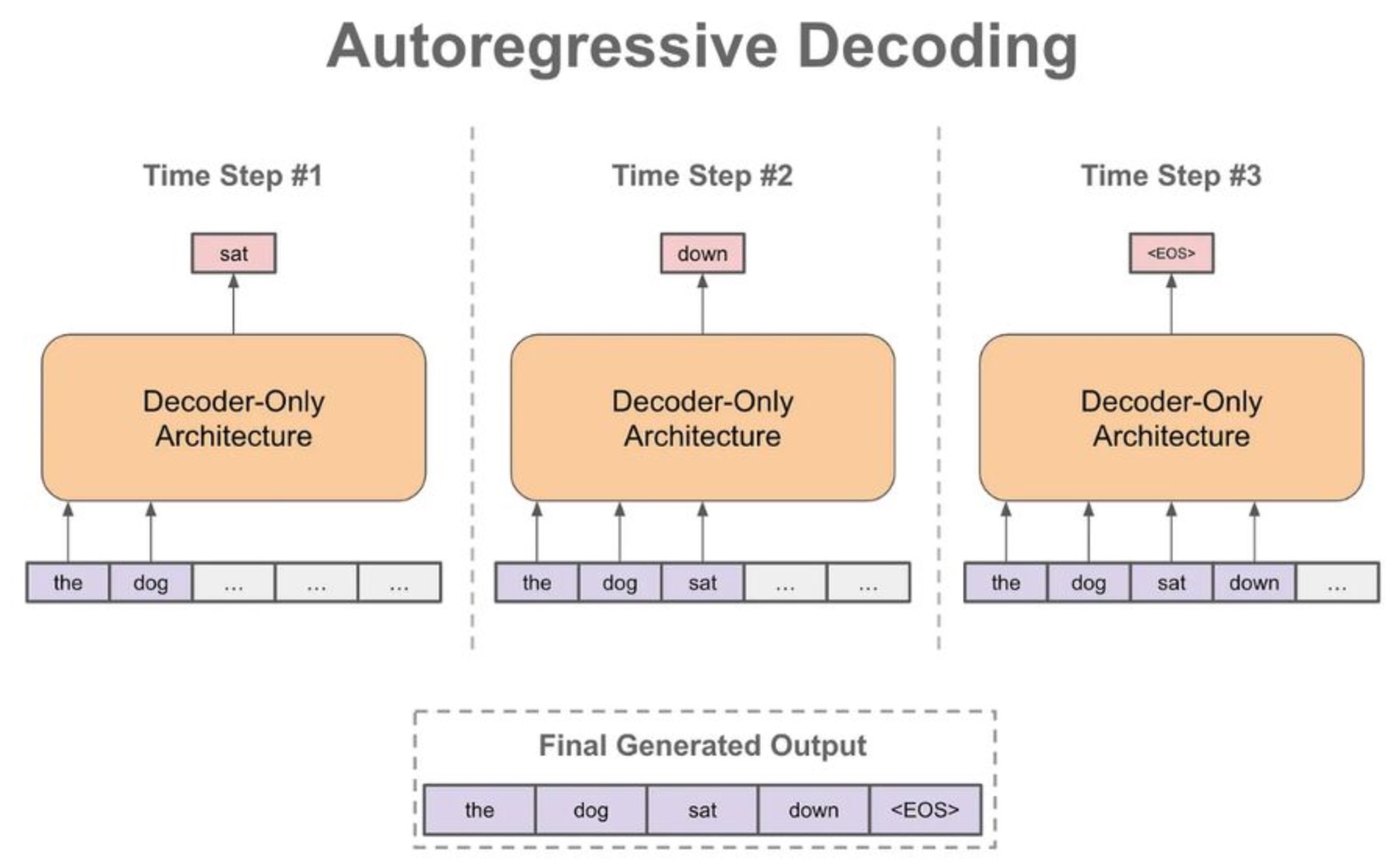
- The simplicity of this formulation is deceptive; despite being a “just next token prediction model,” such autoregressive systems can exhibit remarkable emergent reasoning abilities when scaled, as discussed formally in works like Auto-Regressive Next-Token Predictors Are Universal Learners by Malach (2023).
Token Probabilities
-
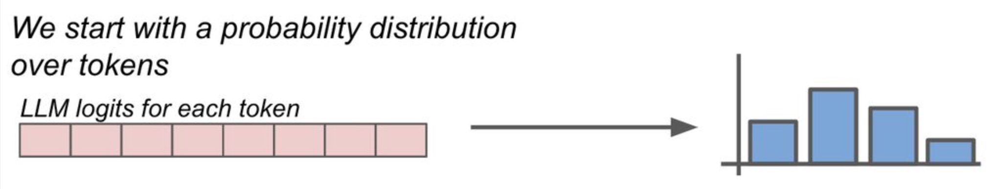
Instead of producing a discrete token directly, an LLM emits a vector of real values called logits for each position in its vocabulary at each timestep. Let \(z=(z_1,\dots,z_n)\) denote the logits for a vocabulary of size \(n\). These logits represent the model’s unnormalized preference for each possible token given the current prefix.
-
To transform logits into a probability distribution over the next token, models apply the softmax function:
\[q_i=\frac{e^{z_i}}{\sum_{j=1}^n e^{z_j}}\]- where \(q_i\) is the probability of the \(i^{\text{th}}\) token. This ensures probabilities are non-negative and sum to 1, allowing a valid categorical interpretation.
-
The resulting probability distribution \(q=(q_1,\dots,q_n)\) expresses how likely each token is as the next one, given the current context. Predicting tokens by sampling from \(q\) or selecting the highest-probability token are different decoding strategies that we will examine later.
-
The role of softmax in normalizing logits to probabilities is visualized below (source):
-
Formally, at time step \(t\), the conditional probability used for sampling or selection is:
\[p(x_t=i\mid x_{<t})=q_i\]- … linking the model’s numerical output (logits) directly to the choice of token during decoding.
Where This Fits in LLM Training and Inference
-
During training, autoregressive models minimize the cross-entropy loss between their predicted probability distributions and the ground-truth next token in large corpora of text. This aligns the model’s parameters to assign high probability to correct next tokens.
-
At inference time (generation), the model no longer knows the true next token and instead must decide how to make a choice based on the learned distribution. This choice is controlled by the decoding strategy (e.g., greedy, sampling, beam search).
-
Whether the model picks the most likely token or samples stochastically can dramatically influence output quality, diversity, and usefulness, as explored in decoding research and empirical studies. Below is the updated “Related: Temperature” section, expanded with additional technical detail, equations, and all original web links retained exactly as in your writeup. I have also added peer-reviewed and authoritative references where appropriate, with correct markdown links, and preserved all image placeholders and captions.
Temperature
-
Although temperature is not itself a decoding strategy, it plays a central role in shaping the behavior of probabilistic decoding methods by modifying the probability distribution from which tokens are selected.
-
Temperature is best understood as a distribution-shaping parameter applied before sampling. It does not change the model’s learned parameters or logits ranking, but instead rescales the logits to control how peaked or flat the resulting probability distribution is.
-
The use of temperature scaling in probabilistic models originates from statistical mechanics and was later adopted in machine learning for calibration and sampling control, including neural language models. Its effect on neural network outputs has been studied in depth in contexts such as probability calibration and confidence estimation, for example in On Calibration of Modern Neural Networks by Guo et al. (2017).
-
In the context of LLMs, temperature is applied during inference only, after the model produces logits but before applying softmax. This means temperature directly affects randomness and diversity of generated text without changing the model’s internal representation or training objective.
-
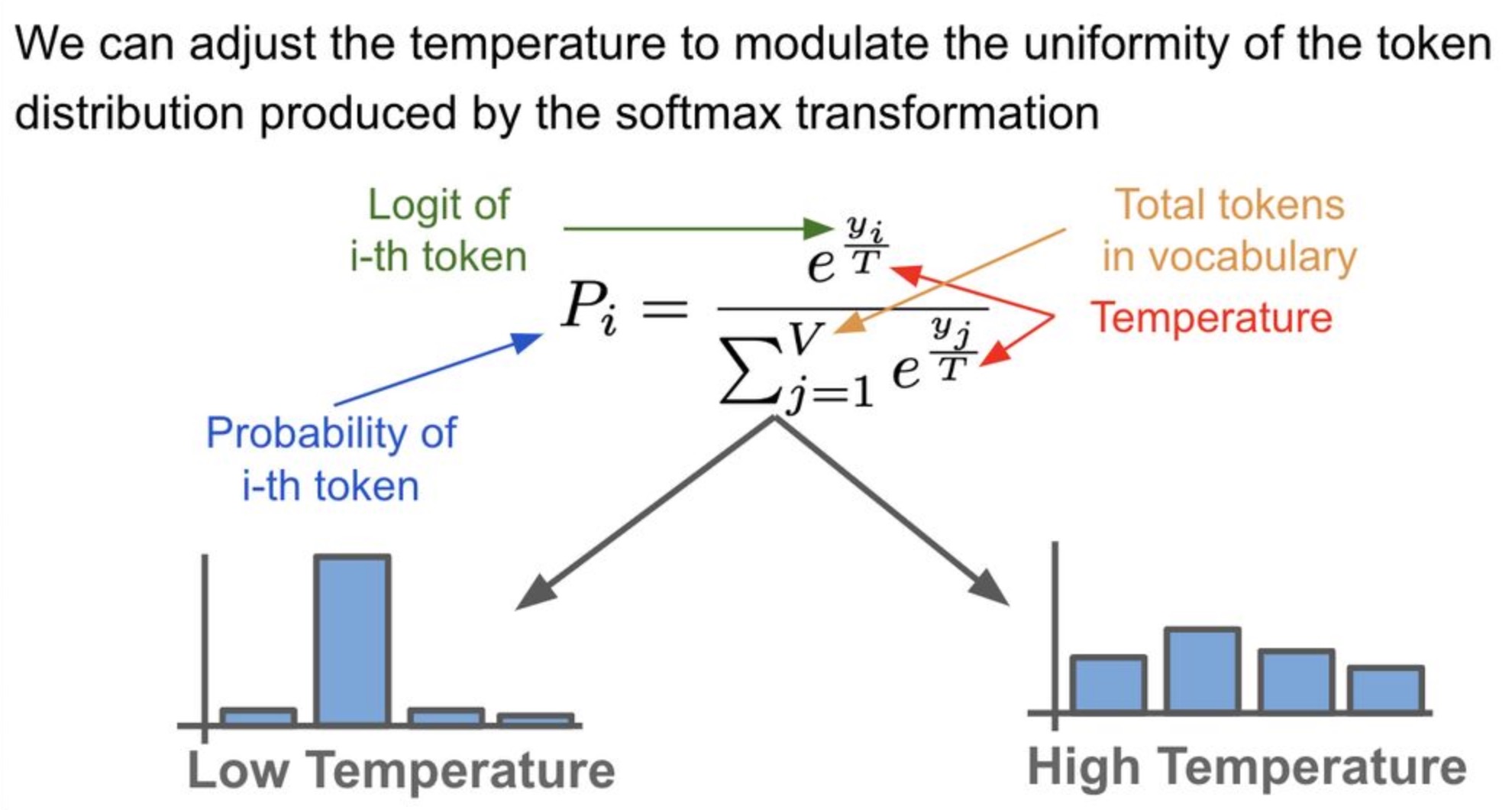
The temperature parameter allows for adjustments to the probability distribution over tokens. It serves as a hyperparameter in the softmax transformation (cf. the image below; source), which governs the randomness of predictions by scaling the logits prior to the application of softmax.
-
For instance, in TensorFlow’s Magenta implementation of LSTMs, the temperature parameter explicitly rescales logits before softmax, demonstrating that temperature-based control is not unique to transformers but applies broadly to autoregressive sequence models.
-
Lower temperature values yield more deterministic outputs, while higher values lead to more creative but less predictable outputs, facilitating a trade-off between determinism and diversity. This trade-off is discussed empirically in The Curious Case of Neural Text Degeneration by Holtzman et al. (2019), where excessive determinism leads to repetitive and degenerate outputs.
The Role of Temperature in Softmax
-
The standard softmax formulation incorporates temperature \(T\) as a scaling factor applied to logits:
\[q_i = \frac{\exp\left(\frac{z_i}{T}\right)}{\sum_{j=1}^{n} \exp\left(\frac{z_j}{T}\right)}\]-
where:
- \(z_i\) is the logit for token \(i\),
- \(T > 0\) is the temperature parameter,
- \(q_i\) is the resulting probability of token \(i\).
-
-
The temperature parameter directly controls the sharpness and entropy of the resulting probability distribution by scaling logits before normalization, thereby influencing how deterministic or exploratory the model’s token selection behavior becomes. This effect can be understood concretely by examining how different temperature regimes alter the relative influence of high- and low-valued logits during sampling:
-
When \(T = 1\), the distribution reduces to the standard softmax, as described in classical neural network literature.
-
When \(T < 1\), the output distribution becomes more sharply peaked, increasing the gap between high- and low-probability tokens and concentrating probability mass on the most likely outcomes. As a result, overall uncertainty (i.e., entropy) are reduced, biasing generation toward more deterministic, greedy choices.
-
When \(T > 1\), the output distribution becomes flatter, decreasing the gap between high- and low-probability tokens and spreading probability mass more evenly across alternatives. As a result, entropy increases, biasing generation toward more exploratory and diverse outputs.
-
-
As \(T \to 0^{+}\), the softmax distribution converges toward a delta distribution centered on the argmax token:
\[\lim_{T \to 0^{+}} q_i = \begin{cases} 1 & \text{if } i = \arg\max_j z_j, \\ 0 & \text{otherwise} \end{cases}\] -
This formalizes why low temperature sampling becomes equivalent to greedy decoding, a fact also noted in decoding strategy analyses such as Neural Text Generation: A Practical Guide by Gatt and Krahmer (2017).
Temperature Ranges and Their Effects
Low Temperature (T \(\approx\) 0.0 – 0.5)
-
Characteristics:
- Strong preference for high-probability tokens.
- Output distributions are sharply peaked.
- Generation becomes nearly deterministic.
-
Applications:
- Suitable for factual question answering, code generation, and tasks where correctness outweighs diversity.
-
Cons:
- Increases risk of repetitive loops and generic responses, a phenomenon documented in decoding failure analyses such as Holtzman et al. (2019).
Moderate Temperature (T \(\approx\) 0.6 – 1.0)
-
Characteristics:
- Balances exploitation (high-probability tokens) and exploration (lower-probability tokens).
- Maintains fluency while introducing controlled variability.
-
Applications:
- Common default range (especially 0.7) for conversational agents, creative writing, and summarization.
-
Cons:
- Still biased toward dominant tokens in highly skewed distributions.
High Temperature (T > 1.0)
-
Characteristics:
- Produces flatter distributions.
- Increases entropy and randomness, improving diversity.
- Allows sampling from a broader portion of the vocabulary.
-
Applications:
- Brainstorming, creative storytelling, and exploratory generation.
-
Cons:
- Higher likelihood of grammatical errors, incoherence, and off-topic outputs.
- May amplify noise present in the tail of the distribution, as discussed in Sampling Strategies for Neural Language Models by Fan et al. (2018).
Insights from the Softmax Function
- From the Wikipedia article on softmax function:
For high temperatures \(\left(\tau \rightarrow \infty\right)\), all samples have nearly the same probability, and the lower the temperature, the more expected rewards affect the probability. For a low temperature \(\left(\tau \rightarrow 0^{+}\right)\), the probability of the sample with the highest expected reward tends to 1.
- This interpretation aligns with both theoretical analysis and empirical observations in LLM decoding research, reinforcing temperature’s role as a continuous knob between deterministic and stochastic generation.
Takeaways
- Temperature rescales logits prior to softmax, reshaping the output probability distribution without altering token rankings.
- Lower temperature values approximate greedy decoding.
- Higher temperature values increase entropy and diversity at the cost of reliability.
- Temperature interacts strongly with other decoding strategies such as top-\(k\) and top-\(p\), although in some APIs (e.g., OpenAI GPT-3), these controls are treated as mutually exclusive.
- Proper tuning of temperature is critical for aligning model behavior with task requirements, making it a foundational control mechanism in practical LLM deployment.
Greedy Decoding
-
Greedy decoding is the simplest and most deterministic decoding strategy used in autoregressive language models. At each timestep, the model selects the token with the highest conditional probability, ignoring all other candidates.
-
Formally, given a probability distribution over the vocabulary \(\mathcal{V}\) at time step \(t\), greedy decoding selects the next token as:
\[x_t = \arg\max_{i \in \mathcal{V}} ; p(x_t = i \mid x_{<t})\]- where \(x_{<t}\) denotes all previously generated tokens. This corresponds to selecting the argmax of the softmax probabilities.
-
Greedy decoding is commonly used as a baseline in neural sequence generation and appears in foundational sequence modeling work such as Sequence to Sequence Learning with Neural Networks by Sutskever et al. (2014).
-
Because greedy decoding always commits to the locally optimal choice, it is myopic: once a token is selected, the model cannot revise it later. This can cause error propagation in tasks like translation or structured generation, where an early locally plausible choice can block the globally best continuation.
-
During decoding, greedy strategies typically continue generating tokens until a special end-of-sequence marker (e.g.,
<END>) is produced. For instance:<START> he hit me with a pie <END> -
Greedy decoding is computationally attractive because it requires only one forward pass per generated token and a maximization over the vocabulary each step, giving a time cost on the order of:
\[O(T \cdot |\mathcal{V}|)\]- where \(T\) is the generated length and \(\|\mathcal{V}\|\) is vocabulary size.
-
Despite its efficiency, greedy decoding often produces suboptimal and repetitive text in open-ended generation. This is analyzed empirically in The Curious Case of Neural Text Degeneration by Holtzman et al. (2019), which shows that always selecting the highest-probability option can lead to blandness and degeneracy in generated sequences.
-
The image below (source) illustrates greedy decoding in action, showing how the model consistently picks the top token at each timestep:
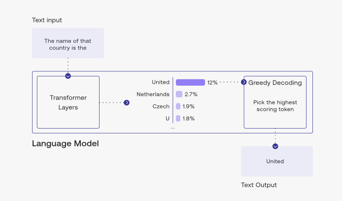
- Because greedy decoding optimizes token-level likelihood rather than exploring alternative continuations, practical systems often prefer strategies that maintain multiple hypotheses, such as beam search, or stochastic approaches like top-\(k\) and top-\(p\) sampling.
Pros and Cons
-
Pros:
- Deterministic and fully reproducible for a given prompt and model.
- Computationally efficient with low latency.
- Simple to implement and easy to reason about.
- Useful as a strong baseline and for debugging model behavior.
- Works well for short, highly constrained, or factual outputs.
-
Cons:
- Myopic decision-making that optimizes only local token probabilities.
- Irreversible error propagation once a suboptimal token is chosen.
- Low diversity and high tendency toward repetitive or generic text.
- Poor performance on open-ended, creative, or long-form generation tasks.
- Often produces degenerate outputs compared to stochastic decoding methods.
Takeaways
- Greedy decoding is deterministic and fast.
- It selects \(\arg\max\) at every timestep.
- It is prone to error propagation and reduced diversity.
- It is mainly used as a baseline or as a component inside more advanced decoding strategies.
Exhaustive Search Decoding
-
Exhaustive search decoding, also known as brute-force decoding, attempts to find the globally optimal output sequence by enumerating all possible token sequences up to a given length and selecting the one with the highest overall probability under the model.
-
Formally, given an autoregressive language model and a maximum sequence length \(T\), exhaustive search aims to solve:
\[x_{1:T}^* = \arg\max_{x_{1:T} \in \mathcal{V}^T} \prod_{t=1}^{T} p(x_t \mid x_{<t})\]- or equivalently, since log is monotonic:
-
This objective explicitly optimizes sequence-level probability, in contrast to greedy decoding, which only optimizes token-level probability at each step.
-
Exhaustive decoding provides a theoretical upper bound on decoding quality, since it guarantees finding the most likely sequence under the model. This idea is discussed in early sequence modeling and probabilistic inference literature, including A Tutorial on Hidden Markov Models and Selected Applications in Speech Recognition by Rabiner (1989), where exhaustive enumeration is presented as a baseline inference method before introducing more efficient alternatives.
-
In the context of neural machine translation and sequence-to-sequence models, exhaustive search has been used primarily as a conceptual reference, not a practical decoding strategy. As the output length grows, the number of possible sequences grows exponentially:
\[|\mathcal{V}|^T\]-
where:
- \(\|\mathcal{V}\|\) is the vocabulary size, often on the order of \(10^4\) to \(10^5\) tokens.
- \(T\) is the sequence length.
-
-
This leads directly to an intractable time complexity:
\[O(|\mathcal{V}|^T)\]- making exhaustive search infeasible for all but trivially small vocabularies or very short sequences.
-
For example, even with a modest vocabulary of 30,000 tokens and a sequence length of 10, the number of possible sequences is:
\[30{,}000^{10} \approx 5.9 \times 10^{44}\]- which is computationally impossible to enumerate.
-
Despite its impracticality, exhaustive search is important conceptually because it clarifies:
- The difference between local and global optimality in decoding
- Why greedy decoding can fail even when each local choice appears optimal
- The motivation for approximate search algorithms like beam search
-
In probabilistic sequence modeling, exhaustive search is often contrasted with dynamic programming or heuristic search methods that approximate the global optimum. This contrast is foundational in decoding theory and is discussed in works such as Neural Machine Translation by Jointly Learning to Align and Translate by Bahdanau et al. (2014), which motivate approximate inference due to the infeasibility of exact search.
-
Because exhaustive search is computationally prohibitive, modern LLM systems never use it in practice. Instead, they rely on:
- Beam search to approximate sequence-level optimization
- Sampling-based methods (top-\(k\), top-\(p\), min-\(p\)) to balance diversity and fluency
- Hybrid strategies that trade optimality for tractability
Pros and Cons
-
Pros:
- Guarantees finding the globally optimal sequence under the model by explicitly maximizing sequence-level probability.
- Serves as a theoretical upper bound on decoding quality, providing a clear reference point for evaluating approximate decoding strategies.
- Clarifies the distinction between local optimality (token-level decisions) and global optimality (sequence-level decisions).
- Provides conceptual motivation for the development of more efficient decoding algorithms such as beam search and heuristic methods.
-
Cons:
- Computationally intractable due to exponential time complexity \(O(\|\mathcal{V}\|^T)\).
- Impossible to use in practice for realistic vocabulary sizes and sequence lengths.
- Requires enumerating an astronomically large search space, even for short outputs.
- Offers no practical trade-off between quality and efficiency, limiting its use to theoretical analysis rather than real-world systems.
Takeaways
- Exhaustive search decoding guarantees the optimal sequence under the model.
- Its complexity grows exponentially with sequence length.
- It is infeasible for real-world language generation.
- It serves as a theoretical baseline motivating approximate decoding strategies.
Beam Search
-
Beam search is a heuristic search algorithm widely used in sequence generation tasks such as neural machine translation, speech recognition, and text generation. It approximates sequence-level optimization while remaining computationally tractable.
-
Unlike greedy decoding, which keeps only a single hypothesis at each timestep, beam search maintains a fixed number of partial hypotheses, called the beam, and expands them in parallel.
-
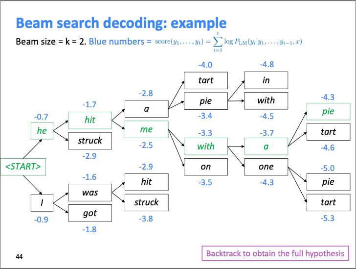
At timestep \(t\), beam search keeps track of the top \(k\) partial sequences (hypotheses) \({h_1, \dots, h_k}\) with the highest cumulative scores, where \(k\) is the beam size.
-
Each hypothesis \(h\) is associated with a cumulative log-probability score:
\[\text{score}(h) = \sum_{i=1}^{t} \log p(x_i \mid x_{<i})\]- where \(x_i\) is the \(i^{\text{th}}\) token in the hypothesis.
-
For a detailed discourse on this topic, please refer D2L.ai: Beam Search.
Steps
- At every decoding timestep, beam search proceeds through three conceptual phases:
Hypothesis expansion
- Each active hypothesis in the beam is expanded by all possible next tokens in the vocabulary \(\mathcal{V}\).
- If the beam contains \(k\) hypotheses, hypothesis generation produces \(k \times \mid \mathcal{V} \mid\) candidate continuations.
- Each candidate represents a unique prefix formed by appending one new token to an existing hypothesis.
Scoring
-
Every expanded candidate is assigned a score by extending the parent hypothesis score with the log-probability of the newly appended token:
\[\text{score}(h') = \text{score}(h) + \log p(x_t \mid x_{<t})\]- where \(h'\) is the expanded hypothesis.
-
Log-probabilities are used to avoid numerical underflow and to convert products of probabilities into sums.
top-\(k\) Selection (Pruning/Compression/Filtering)
- From the \(k \times \|\mathcal{V}\|\) expanded candidates, only the top \(k\) hypotheses with the highest scores are retained.
- All other candidates are discarded, permanently removing them from future consideration.
-
This pruning step is what keeps beam search computationally feasible and distinguishes it from exhaustive search.
- The image below (source) visually illustrates these steps for beam size \(k = 2\), showing how hypotheses are expanded, scored, and pruned at each timestep:
End-of-Sequence Handling
- Hypotheses may emit an
<END>token at different timesteps. -
When a hypothesis generates
<END>:- It is removed from the active beam.
- It is added to a list of completed hypotheses.
-
Beam search continues until:
- A maximum timestep \(T\) is reached, or
- A predefined number of completed hypotheses is collected.
Length Bias and Normalization
- Beam search exhibits length bias because cumulative log-probabilities decrease as sequences grow longer.
-
To correct this, length normalization is often applied:
\[\text{score}_{\text{norm}}(h) = \frac{1}{t^\alpha} \sum_{i=1}^{t} \log p(x_i \mid x_{<i})\]- where \(\alpha \in [0,1]\) controls the normalization strength.
- This technique was popularized in Google’s Neural Machine Translation System by Wu et al. (2016).
Computational Complexity
-
The time complexity of beam search is approximately:
\[O(T \cdot k \cdot |\mathcal{V}|)\]- making it significantly more expensive than greedy decoding but far more efficient than exhaustive search.
Pros and Cons
-
Pros:
- Approximates sequence-level optimization better than greedy decoding.
- Maintains multiple hypotheses, reducing early commitment errors.
- Deterministic and reproducible given fixed parameters.
- Widely used and well-understood in structured generation tasks.
-
Cons:
- Not guaranteed to find the globally optimal sequence.
- Larger beam sizes do not necessarily improve quality and may degrade results, as shown in On the Inadequacy of Beam Search for Neural Machine Translation by Koehn and Knowles (2017).
- Tends to favor high-probability, generic outputs.
- Computationally expensive for large vocabularies and beam sizes.
- Limited diversity compared to stochastic decoding methods such as top-\(k\) and top-\(p\) sampling.
Takeaways
- Beam search maintains multiple hypotheses to approximate global optimization.
- Each timestep consists of expansion, scoring, and selection (pruning).
- Length normalization is crucial to mitigate bias toward short sequences.
- Beam search balances quality and efficiency but lacks diversity and optimality guarantees.
Constrained Beam Search
-
Constrained beam search is an extension of standard beam search that introduces explicit constraints on the generated output sequence. These constraints enforce that certain conditions are satisfied in the final output, such as including specific tokens, phrases, or structural patterns.
-
This decoding strategy is particularly useful in tasks like neural machine translation, text summarization, data-to-text generation, and dialogue systems, where the output must obey lexical, semantic, or formatting requirements.
-
The motivation for constrained beam search arises from the observation that unconstrained decoding methods, including standard beam search, optimize only likelihood under the model and provide no guarantees about satisfying external requirements. This limitation is discussed in constrained decoding literature such as Lexically Constrained Decoding for Sequence Generation Using Grid Beam Search by Hokamp and Liu (2017).
Core Idea
-
The central idea of constrained beam search is to modify the beam expansion and pruning process so that constraints are respected throughout decoding.
-
Constraints can be hard or soft:
- Hard constraints must be satisfied for a sequence to be valid.
- Soft constraints are encouraged via penalties or bonuses but may be violated if necessary.
-
Let \(\mathcal{C}\) denote a set of constraints. The decoding objective becomes:
\[x_{1:T}^* = \arg\max_{x_{1:T} \in \mathcal{V}^T} \sum_{t=1}^{T} \log p(x_t \mid x_{<t}) \quad \text{subject to } x_{1:T} \models \mathcal{C}.\] -
This formulation explicitly separates sequence likelihood from constraint satisfaction, requiring decoding algorithms to account for both simultaneously.
Steps
- At each decoding timestep, constrained beam search follows the same high-level structure as standard beam search, but with constraint-aware modifications.
Hypothesis generation
- Each hypothesis in the beam is expanded by all possible next tokens.
- In addition to token probabilities, each expanded hypothesis tracks a constraint state, representing which constraints have been satisfied so far.
Scoring
-
Expanded hypotheses are scored using cumulative log-probabilities, optionally augmented with constraint-related bonuses or penalties:
\[\text{score}(h) = \sum_{i=1}^{t} \log p(x_i \mid x_{<i}) + \lambda \cdot f_{\text{constraint}}(h),\]-
where:
- \(f_{\text{constraint}}(h)\) measures progress toward satisfying constraints,
- \(\lambda\) controls the influence of constraints on scoring.
-
-
This approach allows constrained decoding to trade off fluency against constraint satisfaction when soft constraints are used.
Pruning (top-\(k\) Selection/Compression/Filtering)
- Hypotheses that violate hard constraints are immediately pruned.
- Remaining hypotheses are grouped or ranked based on both likelihood and constraint satisfaction.
-
Only the top \(k\) hypotheses are retained, ensuring tractability.
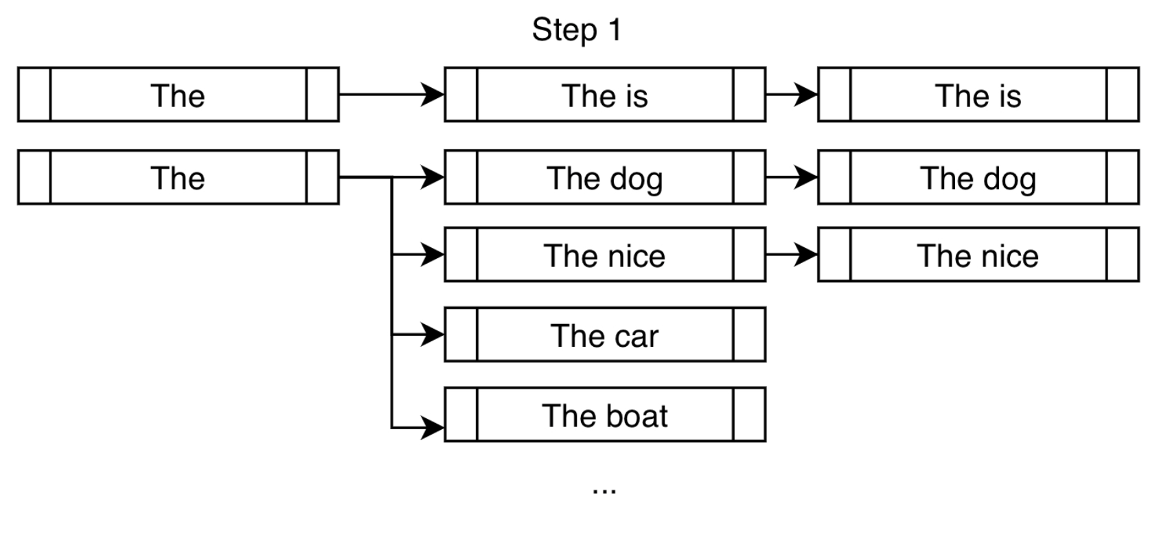
- The image below (source) illustrates constrained beam search at an early timestep. In addition to high-probability tokens like “dog” and “nice,” the token “is” is forced to satisfy the constraint “is fast.” (source)
Banking Mechanism
-
A common implementation of constrained beam search uses a banking mechanism, which groups hypotheses into banks based on how many constraints they have satisfied.
-
Let bank \(B_i\) contain hypotheses that have satisfied exactly \(i\) constraints.
-
During pruning, hypotheses are selected in a round-robin fashion across banks to maintain diversity while ensuring progress toward satisfying constraints.
-
This approach was formalized and popularized in Hugging Face’s implementation and documentation of constrained beam search, which builds on earlier work such as Hokamp and Liu (2017).
-
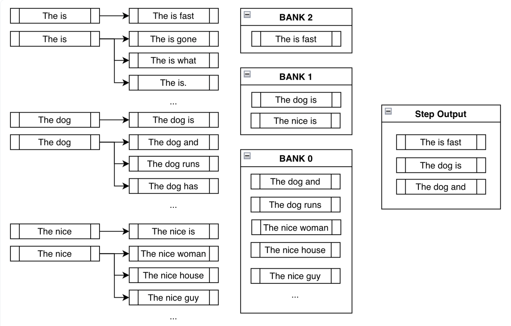
The image below (source) shows how hypotheses are organized into banks and selected alternately:
Example Selection via Banking
-
After sorting hypotheses into banks, selection proceeds cyclically:
- Choose the highest-scoring hypothesis from the most constrained bank.
- Then choose from less constrained banks.
- Repeat until the beam is filled.
-
As described in the original example (source):
“After sorting all the possible beams into their respective banks, we do a round-robin selection… ending up with
["The is fast", "The dog is", "The dog and"].” -
This ensures that constraint satisfaction does not completely override fluency, and vice versa.
-
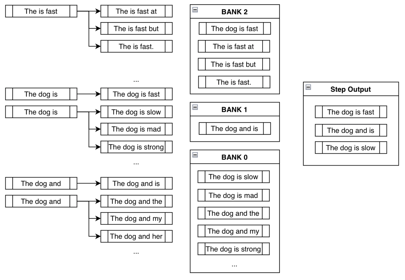
The final combined result is illustrated below (source):
Pros and Cons
-
Pros:
- Guarantees satisfaction of hard constraints.
- Enables controllable generation.
- Maintains fluency through likelihood-based scoring.
-
Cons:
- Higher computational cost than standard beam search.
- Requires careful constraint specification.
- Can still generate unnatural phrasing if constraints conflict with model priors.
Takeaways
- Constrained beam search extends beam search with explicit constraint tracking.
- Hypotheses are expanded, scored, and pruned with respect to both probability and constraints.
- Banking mechanisms balance constraint satisfaction with linguistic quality.
- This method is essential for structured and controlled text generation tasks.
Top-\(k\) Sampling
-
Top-\(k\) sampling is a stochastic decoding strategy that restricts token selection to a fixed-size subset of the most probable tokens at each decoding step.
-
Instead of considering the entire vocabulary \(\mathcal{V}\), the model first selects the \(k\) tokens with the highest conditional probabilities and then samples from this reduced set.
-
This method was introduced to address the lack of diversity produced by deterministic decoding methods such as greedy decoding and beam search, and is discussed in early neural text generation work such as Hierarchical Neural Story Generation by Fan et al. (2018) and later formalized in decoding analyses like The Curious Case of Neural Text Degeneration by Holtzman et al. (2019).
Definition
-
Let \(p(x_t \mid x_{<t})\) be the model’s probability distribution over the vocabulary at timestep \(t\).
-
Define \(\mathcal{V}_k \subseteq \mathcal{V}\) as the set of the \(k\) tokens with the highest probabilities:
\[\mathcal{V}_k = \operatorname{TopK}\left(p(x_t \mid x_{<t}), k\right)\] -
All tokens not in \(\mathcal{V}_k\) are discarded by setting their probability mass to zero.
-
The remaining probabilities are renormalized:
\[\tilde{p}(x_t=i) = \begin{cases} \frac{p(x_t=i)}{\sum_{j \in \mathcal{V}_k} p(x_t=j)} & i \in \mathcal{V}_k, \ 0 & \text{otherwise} \end{cases}\] -
The next token is then sampled from \(\tilde{p}\).
Hypothesis Generation, Scoring, and top-\(k\) Selection Perspective
-
Hypothesis generation: The full vocabulary is initially considered.
-
Scoring: Tokens are ranked by probability.
-
Top-\(k\) Selection: Only the top \(k\) tokens are retained; all others are pruned before sampling.
-
Unlike beam search, top-\(k\) sampling does not maintain multiple hypotheses across timesteps. Instead, it introduces randomness at each timestep independently.
Uniform vs. Probability-Weighted Sampling
-
The choice between uniform and probability-weighted sampling in top-\(k\) decoding reflects a tradeoff between diversity and faithfulness to the model’s learned distribution.
-
In top-\(k\) sampling, once the \(k\) highest-probability tokens are selected, the actual draw can be performed in two main ways:
- Uniform sampling, where each of the \(k\) candidates is assigned probability \(\frac{1}{k}\).
- Probability-weighted sampling, where the original model probabilities over the \(k\) tokens are renormalized and sampled proportionally.
-
Uniform sampling over the top-\(k\) set intentionally flattens the distribution, increasing lexical diversity but often degrading coherence and factual accuracy. On the other hand, probability-weighted sampling biases generation toward more contextually appropriate tokens while still allowing stochastic exploration.
-
When probability-weighted sampling is used after filtering, top-\(k\) and top-\(p\) decoding share the same downstream sampling procedure and differ only in how the candidate token set is constructed, as described in The Curious Case of Neural Text Degeneration by Holtzman et al. (2019).
-
In practice, top-\(k\) sampling almost always uses probability-weighted sampling. This formulation was introduced in early neural text generation work and is used by default in most modern implementations, because it preserves the model’s relative confidence among retained tokens while truncating the long tail. See On the Diversity of Sampling Strategies for Neural Text Generation by Fan et al. (2018) and The Curious Case of Neural Text Degeneration by Holtzman et al. (2019).
-
For implementation details and concrete code examples of probability-weighted sampling, see the Related: Sampling from a Probability Distribution section, as well as How to generate text: using different decoding methods for language generation and Sampling from a Probability Distribution.
Example: Top-\(k\) with \(k = 3\)
- Assume the model outputs the following probabilities for the next token:
- The top-\(k\) tokens for \(k = 3\) are \({A, B, C}\).
Uniform Sampling
- Each of the three tokens is assigned equal probability:
- Token \(C\) (original probability 0.15) is sampled just as often as token \(A\) (original probability 0.50).
- This increases lexical diversity but may introduce less coherent or less likely continuations.
Probability (Renormalized) Sampling
- Probabilities are renormalized over the selected tokens:
- Higher-probability tokens remain more likely to be selected.
- This preserves coherence while still allowing variation.
Comparison to Greedy Decoding
-
Greedy decoding does not perform sampling and always selects the token corresponding to the highest probability. Put simply, it implicitly assigns probability 1 to the most likely token and 0 to all others by selecting:
\[x_t = \arg\max_i p(x_t=i \mid x_{<t})\] -
As a result, greedy decoding emphasizes likelihood maximization exclusively, eliminating randomness and diversity. The downside is that this often leads to repetitive or generic outputs.
Behavior at Extreme Values of \(k\)
-
When \(k = 1\):
- The candidate set contains only the most probable token, making sampling deterministic.
-
Top-\(k\) sampling reduces exactly to greedy decoding:
\[x_t = \arg\max_i p(x_t=i \mid x_{<t})\]
-
When \(k = \|\mathcal{V}\|\):
- No filtering occurs.
- Sampling is equivalent to drawing directly from the full softmax distribution.
-
These edge cases show that top-\(k\) sampling smoothly interpolates between greedy decoding and unconstrained sampling.
Practical Implications
-
Smaller values of \(k\):
- Reduce randomness.
- Increase fluency and determinism.
- Risk repetitive or generic output.
-
Larger values of \(k\):
- Increase diversity.
- Allow exploration of lower-probability tokens.
- Risk incoherence or semantic drift.
-
The image below (source) illustrates top-\(k\) sampling for \(k = 3\):
Pros and Cons
-
Pros:
- Simple and efficient to implement.
- Improves diversity over greedy decoding.
- Provides explicit control over candidate set size.
-
Cons:
- Requires manual tuning of \(k\).
- Fixed \(k\) is suboptimal when the probability distribution is highly skewed.
- Can still include low-quality tokens if they fall within the top \(k\).
-
These limitations motivate adaptive approaches such as nucleus (top-\(p\)) sampling, which dynamically adjusts the candidate set size based on cumulative probability mass.
Takeaways
- Top-\(k\) sampling restricts token selection to the \(k\) most probable tokens.
- Sampling occurs after filtering and renormalization.
- \(k\) controls the diversity–coherence trade-off.
- \(k = 1\) reduces to greedy decoding.
- Top-\(k\) sampling is a foundational stochastic decoding method and a precursor to more adaptive strategies.
Top-\(p\) (Nucleus Sampling)
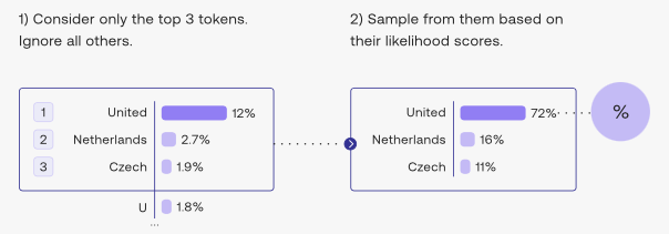
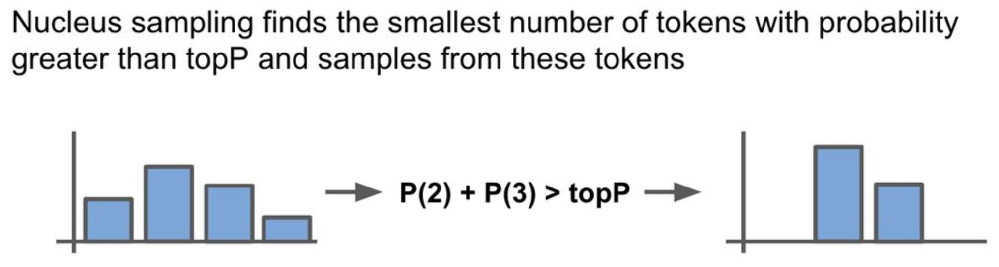
- Top-\(p\) sampling, also known as nucleus sampling, is a stochastic decoding strategy designed to address the limitations of fixed-size candidate filtering methods such as top-\(k\).
- Instead of selecting a fixed number of tokens, nucleus sampling dynamically selects a variable-sized subset of tokens whose cumulative probability mass exceeds a threshold \(p\).
- This approach was introduced and formalized in The Curious Case of Neural Text Degeneration by Holtzman et al. (2019), where the authors demonstrate that sampling from the probability “nucleus” avoids degenerate and repetitive text produced by deterministic or poorly tuned sampling strategies.
- In top-\(p\) sampling, probability-weighted sampling is always used after the nucleus is constructed, since the candidate set itself is defined in terms of cumulative probability mass. The probability-weighted sampling process itself is described in the Uniform vs. Probability-Weighted Sampling section.
Definition
-
Let \(p(x_t \mid x_{<t})\) be the model’s probability distribution over the vocabulary \(\mathcal{V}\) at timestep \(t\).
-
Tokens are first sorted in descending order of probability:
\[p_1 \ge p_2 \ge \dots \ge p_{|\mathcal{V}|}\] -
Define the nucleus \(\mathcal{V}_p\) as the smallest subset of tokens such that their cumulative probability mass exceeds \(p\):
\[\mathcal{V}_p = \left{ i | \sum_{j=1}^{i} p_j \ge p \right}\] -
All tokens outside \(\mathcal{V}_p\) are discarded.
-
The remaining probabilities are renormalized:
\[\tilde{p}(x_t=i) = \begin{cases} \frac{p(x_t=i)}{\sum_{j \in \mathcal{V}_p} p(x_t=j)} & i \in \cal{V}_p, \\ 0 & \text{otherwise} \end{cases}\] -
The next token is sampled from this renormalized distribution.
Intuition
-
Fixed \(k\) in top-\(k\) sampling can be problematic:
- When the distribution is sharply peaked, even small \(k\) may include low-quality tokens.
- When the distribution is flat, small \(k\) may exclude plausible continuations.
-
Nucleus sampling solves this by adapting the candidate set size to the shape of the distribution, ensuring that:
- Only high-probability mass is considered.
- The long tail of extremely low-probability tokens is excluded.
-
This adaptive behavior is the key insight behind nucleus sampling and the reason it often produces more coherent and human-like text than top-\(k\) alone.
-
The image below (source) illustrates nucleus sampling in action:
How Is Nucleus Sampling Useful?
-
Top-\(p\) sampling is particularly effective for tasks requiring fine-grained control over diversity and fluency, such as open-ended language modeling, text summarization, and dialogue generation.
-
In practice, \(p\) is typically set relatively high (often around 0.7–0.9, commonly ≈ 0.75) to exclude only the low-probability tail while preserving most plausible continuations.
-
Consider two contrasting cases:
- Highly peaked distribution: If a single token has probability greater than \(p\), the nucleus contains only that token. Sampling becomes deterministic and equivalent to greedy decoding.
- Flat distribution: Many tokens are required to reach cumulative probability \(p\), so the nucleus grows larger, allowing more diversity.
-
This dynamic adjustment allows nucleus sampling to automatically respond to the model’s uncertainty at each timestep.
-
Additionally, top-\(k\) and top-\(p\) can be combined:
- First apply top-\(k\) filtering.
- Then apply top-\(p\) filtering on the reduced set.
- In this configuration, \(p\) is always applied after \(k\), ensuring both an upper bound on candidate count and a probability-mass constraint.
Relationship to Greedy Decoding and Top-\(k\)
-
Edge cases clarify the relationship between decoding methods:
- If \(p \to 0\), nucleus sampling collapses to greedy decoding.
- If \(p \to 1\), nucleus sampling approaches unrestricted sampling from the full softmax distribution.
-
Compared to top-\(k\):
- Top-\(k\) uses a fixed number of tokens regardless of probability mass.
- Top-\(p\) uses a variable number of tokens based on cumulative probability.
Nucleus Sampling v/s Temperature
-
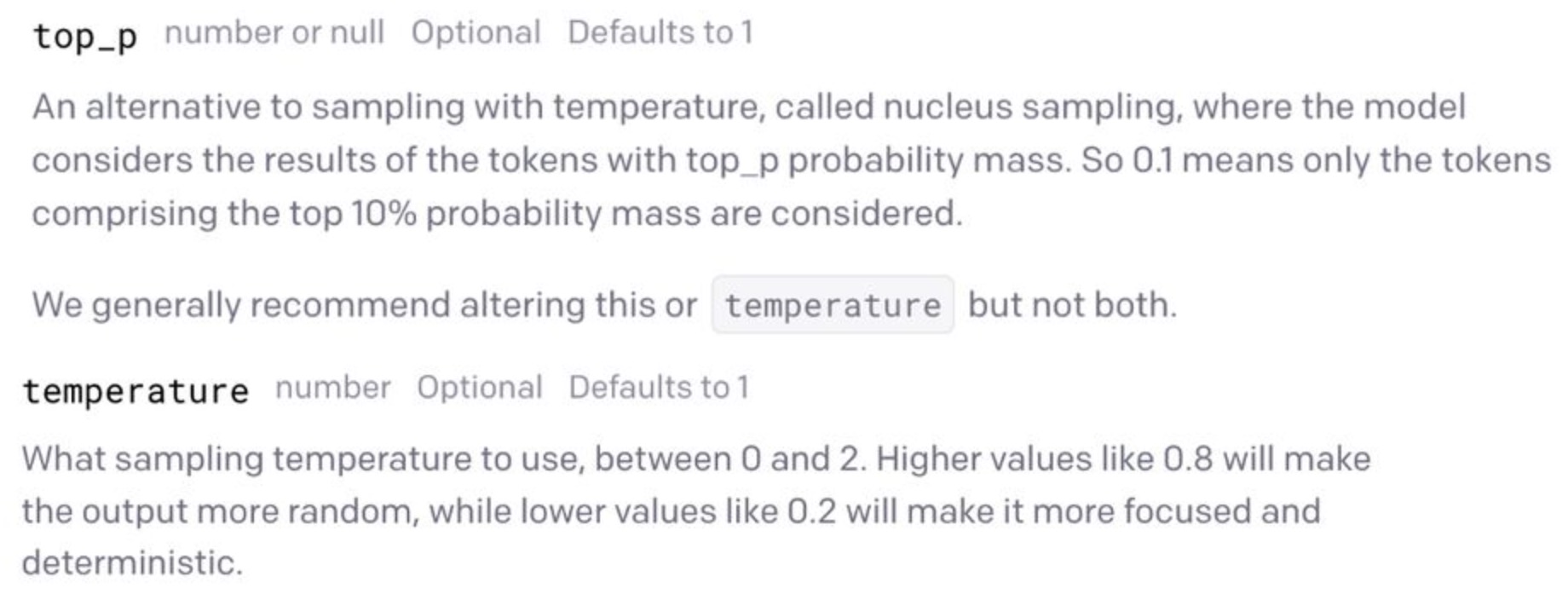
Based on OpenAI’s GPT-3 API, temperature and nucleus sampling are treated as alternative mechanisms for controlling randomness and should not be used simultaneously.
-
Conceptually:
- Temperature rescales the entire probability distribution by modifying logits before softmax.
- Top-\(p\) truncates the distribution after softmax by removing low-probability tokens.
-
Because they affect different stages of decoding, combining them can produce unintuitive or unstable behavior. For this reason, many APIs enforce mutual exclusivity between temperature-based sampling and nucleus sampling.
-
The image below (source) illustrates this API-level distinction:
Pros and Cons
-
Pros:
- Adaptive candidate set size.
- Strong balance between diversity and coherence.
- Robust to distribution skewness.
- Empirically shown to reduce text degeneration.
-
Cons:
- Requires tuning of \(p\).
- Still stochastic and non-deterministic.
- Can collapse to greedy behavior when distributions are highly peaked.
Takeaways
- Nucleus sampling selects the smallest set of tokens whose cumulative probability exceeds \(p\).
- It dynamically adapts to the model’s uncertainty.
- It avoids low-probability tail sampling while preserving diversity.
- It generalizes top-\(k\) sampling and can be combined with it.
- It is one of the most widely used decoding strategies in modern LLM systems.
Greedy vs. Top-\(k\) and Top-\(p\)
- Decoding strategies fundamentally differ in how they trade off determinism, diversity, and risk. Greedy decoding, top-\(k\) sampling, and top-\(p\) (nucleus) sampling represent three points along a spectrum from fully deterministic to controlled stochastic generation.
Deterministic vs. Stochastic Decoding
-
Greedy decoding is fully deterministic. At each timestep, it selects:
\[x_t = \arg\max_i p(x_t=i \mid x_{<t})\]- guaranteeing the same output for the same prompt and model parameters.
-
Top-\(k\) and top-\(p\) sampling are stochastic. Instead of selecting the single most probable token, they:
- Restrict the candidate set (by count or probability mass).
- Sample randomly from the remaining distribution.
-
This stochasticity explains why repeated generations from the same prompt can yield different outputs in systems such as ChatGPT, even when the model itself is unchanged.
Search Space Control
-
Greedy decoding:
- Considers the entire vocabulary.
- Selects exactly one token.
- Discards all alternative continuations immediately.
-
Top-\(k\) sampling:
- Restricts the candidate set to exactly \(k\) tokens.
- The size of the candidate set is fixed, regardless of distribution shape.
-
Top-\(p\) sampling:
- Restricts the candidate set to a variable number of tokens.
- The size adapts dynamically to the entropy of the distribution.
-
This distinction is critical in practice. As shown in The Curious Case of Neural Text Degeneration by Holtzman et al. (2019), fixed candidate sets (top-\(k\)) can be brittle, while adaptive sets (top-\(p\)) better reflect model uncertainty.
Error Propagation and Recovery
-
Greedy decoding:
- Suffers from irreversible error propagation.
- A poor early decision cannot be corrected later.
- This often leads to repetitive or incomplete outputs.
-
Top-\(k\) and top-\(p\) sampling:
- Allow occasional low-probability but semantically valid tokens.
- Enable recovery from early suboptimal choices.
- Produce more varied and human-like text.
-
This behavior is particularly important in long-form generation and dialogue, where early rigidity compounds over time.
Bias in Generated Text
-
Greedy decoding tends to produce:
- Safe, generic, high-probability phrases.
- Low lexical and semantic diversity.
- Repetitive structures.
-
Top-\(k\) sampling:
- Improves diversity.
- Can still suffer from unnatural jumps if \(k\) is too large.
-
Top-\(p\) sampling:
- Reduces sampling from the low-probability tail.
- Produces more coherent diversity by construction.
- Is more robust across different probability distributions.
-
These empirical behaviors are consistent with findings in neural generation research and motivate the widespread adoption of nucleus sampling in modern APIs.
Practical Usage Patterns
-
Greedy decoding is commonly used for:
- Debugging
- Baselines
- Short, factual outputs
-
Top-\(k\) sampling is useful when:
- A hard upper bound on randomness is desired
- The distribution shape is relatively stable
-
Top-\(p\) sampling is preferred when:
- Output quality and diversity both matter
- The model’s uncertainty varies across timesteps
- Long-form or open-ended generation is required
-
As mentioned in OpenAI’s GPT-3 API description, modern systems typically expose stochastic sampling parameters rather than greedy decoding alone.
Takeaways
- Greedy decoding is deterministic, efficient, and brittle.
- Top-\(k\) sampling introduces controlled randomness with a fixed candidate set.
- Top-\(p\) sampling introduces adaptive randomness based on probability mass.
- Stochastic methods trade exact likelihood maximization for diversity, robustness, and human-perceived quality.
- In practice, top-\(p\) sampling has become the default decoding strategy for many large language model applications.
min-\(p\) Sampling
-
min-\(p\) sampling is a recent decoding strategy introduced in the Hugging Face Transformers ecosystem to address limitations observed in both top-\(k\) and top-\(p\) sampling.
-
It was proposed and discussed in the Hugging Face community, with the original motivation and design documented in the Transformers issue tracker (Release notes), accompanying discussion (Discussion thread), and example usage (Sample usage).
-
The core goal of min-\(p\) sampling is to dynamically filter low-quality tokens while avoiding two common failure modes:
- Arbitrary truncation by rank (top-\(k\)).
- Inclusion of extremely low-probability tokens due to cumulative mass effects (top-\(p\)).
Background on Existing Sampling Strategies
-
Top-\(k\) sampling:
- Sorts tokens by probability.
- Retains only the top \(k\) tokens.
- Discards all others regardless of their relative probability.
- Can remove high-quality continuations when \(k\) is too small.
-
Top-\(p\) (nucleus) sampling:
- Retains the smallest set of tokens whose cumulative probability exceeds \(p\).
- Adapts to distribution shape.
- May still include tokens with extremely low individual probabilities if the distribution is flat.
-
These limitations are especially problematic at high temperature, where probability mass spreads across many tokens.
Core Idea of min-\(p\) Sampling
-
min-\(p\) sampling introduces a relative probability threshold tied to the most likely token rather than an absolute rank or cumulative mass.
-
Let:
- \(p_{\max} = \max_i p(x_t=i \mid x_{<t})\) be the highest token probability.
- \(\text{min-p} \in (0,1)\) be a user-defined factor.
-
The minimum acceptable probability threshold is defined as:
\[\tau = \text{min-p} \cdot p_{\max}\] -
Only tokens whose probabilities exceed this threshold are retained:
\[\mathcal{V}_{\text{min-p} = \left{i \mid p(x_t=i \mid x_{<t}) \ge \tau \right}\] -
All tokens outside this set are discarded.
-
The remaining probabilities are renormalized and sampled from.
Algorithm
-
Filtering:
- Compute \(p_{\max}\).
- Remove all tokens with probability less than \(\text{min-p} \cdot p_{\max}\).
-
Renormalization:
- Adjust remaining probabilities so they sum to 1.
-
Sampling:
- Draw the next token proportionally from the filtered distribution.
-
This mechanism ensures that:
- Tokens that are orders of magnitude less likely than the best candidate are never sampled.
- The candidate set automatically expands or contracts based on distribution sharpness.
Behavior in Different Probability Landscapes
-
Dominant token present:
- \(p_{\max}\) is much larger than other probabilities.
- Threshold \(\tau\) is high.
- Aggressive filtering occurs.
- Behavior approaches greedy decoding.
-
Flat distribution:
- \(p_{\max}\) is not much larger than other probabilities.
- Threshold \(\tau\) is low.
- Many plausible tokens are retained.
- Sampling remains diverse.
-
This adaptivity is what allows min-\(p\) sampling to perform well under high temperature, where top-\(p\) alone may admit noisy tail tokens.
Relationship to Temperature
-
min-\(p\) sampling is often used together with higher temperatures.
-
Temperature controls how spread-out the distribution is.
-
min-\(p\) controls how much of the low-probability tail is allowed after that spread.
-
This pairing is especially powerful:
- Temperature increases creativity.
- min-\(p\) prevents incoherence.
-
As noted in the Hugging Face discussion, min-\(p\) can reduce or eliminate the need for heuristic techniques such as repetition penalties, because it naturally suppresses implausible continuations.
Recommended Settings
-
Practical guidance from the Hugging Face community suggests:
- \[\text{min-p} \in [0.05, 0.1]\]
- Temperature \(> 1.0\) for creative generation
-
This configuration allows:
- Broad exploration of ideas.
- Automatic suppression of very unlikely tokens.
- More stable and coherent long-form outputs.
Pros and Cons
-
Pros:
- Adaptive to distribution shape.
- Robust under high temperature.
- Prevents sampling of extremely low-probability tokens.
- Works well for creative generation.
-
Cons:
- Still stochastic and non-deterministic.
- Requires tuning of an additional hyperparameter.
- Less theoretically studied than top-\(k\) or top-\(p\).
Takeaways
- min-\(p\) sampling filters tokens based on a relative probability threshold tied to the most likely token.
- It generalizes and complements top-\(k\) and top-\(p\) sampling.
- It is especially effective in high-entropy decoding regimes.
- min-\(p\) offers a principled way to increase creativity while maintaining coherence.
- It represents a promising direction for future decoding strategy research and practice.
Comparative Analysis
- Deterministic methods (greedy, beam-based) optimize likelihood but often sacrifice diversity.
- Stochastic methods (top-\(k\), top-\(p\), min-\(p\)) trade exact optimality for diversity and robustness.
- Adaptive strategies (top-\(p\), min-\(p\)) respond better to changing uncertainty in the model’s probability distribution.
- Temperature is not a decoding strategy by itself but a global modifier that reshapes distributions before decoding.
- In practice, top-\(p\) and min-\(p\) sampling dominate modern open-ended generation, while beam-based methods remain important for constrained and structured tasks.
Related: Sampling from a Probability Distribution
Overview
- All decoding strategies discussed above ultimately rely on sampling from a probability distribution over tokens.
- Greedy decoding, top-\(k\), top-\(p\), and min-\(p\) differ mainly in how they filter or reshape that distribution before a final selection is made.
- Once a probability distribution is fixed, the actual act of choosing a token is a standard categorical sampling problem.
- Understanding sampling with and without replacement clarifies:
- Why greedy decoding is deterministic
- Why top-\(k\) and top-\(p\) are stochastic
- How filtering and renormalization work internally
-
This section demonstrates these ideas using simple code examples that mirror what happens inside an LLM decoder at a single timestep.
- We will use the same toy distribution throughout:
- Sampling 3 times corresponds to drawing multiple candidate tokens from this distribution.
Sampling with Replacement
- Sampling with replacement means each draw is independent. This matches how LLMs sample tokens across timesteps: once a token is sampled, the model moves forward and generates a new distribution rather than removing that token from consideration.
Plain Python (random.choices)
import random

values = ["A", "B", "C", "D"]
probs = [0.50, 0.30, 0.15, 0.05]

# Draw 3 samples independently using weighted probabilities
samples = random.choices(values, weights=probs, k=3)

print(samples)
-
Key points:
random.choicesperforms categorical sampling- replacement is implicit
- the same token may appear multiple times
NumPy
import numpy as np

values = np.array(["A", "B", "C", "D"])
probs = np.array([0.50, 0.30, 0.15, 0.05])

# replace=True means sampling with replacement
samples = np.random.choice(values, size=3, p=probs, replace=True)

print(samples)
Key points:
pspecifies the probability distributionreplace=Truemirrors repeated independent draws
PyTorch
import torch

values = torch.tensor([0, 1, 2, 3])  # indices representing A, B, C, D
probs = torch.tensor([0.50, 0.30, 0.15, 0.05])

# multinomial samples indices according to probs
samples = torch.multinomial(probs, num_samples=3, replacement=True)

print(samples)
- Mapping indices to labels:
labels = ["A", "B", "C", "D"]

# Convert tensor indices to human-readable labels
sampled_labels = [labels[i] for i in samples.tolist()]

print(sampled_labels)
-
Connection to LLMs:
torch.multinomialis effectively what happens after top-\(k\) or top-\(p\) filtering- Greedy decoding would skip sampling and directly choose
argmax
Sampling without Replacement
-
Sampling without replacement means once a value is chosen, it cannot be chosen again. Probabilities must be renormalized after each draw.
-
This is conceptually similar to selecting a shortlist of tokens during top-\(k\) or top-\(p\) filtering, though LLMs typically sample only one token per timestep.
Plain Python (iterative weighted sampling)
import random

values = ["A", "B", "C", "D"]
probs = [0.50, 0.30, 0.15, 0.05]

samples = []

for _ in range(3):
    # Sample one value using current probabilities
    choice = random.choices(values, weights=probs, k=1)[0]

    # Record the sampled value
    samples.append(choice)

    # Remove the chosen value
    idx = values.index(choice)
    values.pop(idx)
    probs.pop(idx)

    # Renormalize probabilities to sum to 1
    total = sum(probs)
    probs = [p / total for p in probs]

print(samples)
-
Key points:
- sampling happens one step at a time
- probabilities are renormalized after removal
- this mirrors how filtered distributions are handled internally
NumPy
import numpy as np

values = np.array(["A", "B", "C", "D"])
probs = np.array([0.50, 0.30, 0.15, 0.05])

# replace=False enforces no repeated values
samples = np.random.choice(values, size=3, p=probs, replace=False)

print(samples)
-
Key points:
- NumPy handles renormalization internally
- probabilities are interpreted as selection weights
PyTorch
import torch

values = torch.tensor([0, 1, 2, 3])
probs = torch.tensor([0.50, 0.30, 0.15, 0.05])

# replacement=False prevents reusing indices
samples = torch.multinomial(probs, num_samples=3, replacement=False)

print(samples)
- Mapping indices to labels:
labels = ["A", "B", "C", "D"]

sampled_labels = [labels[i] for i in samples.tolist()]

print(sampled_labels)
Pure Python Implementation (No Libraries)
- This section shows the sampling logic itself, independent of any helper libraries. The only requirement is a source of uniform random numbers in \([0,1)\).
Simple uniform random number generator
# Linear congruential generator for reproducible uniform randomness
def lcg(seed):
    a = 1664525
    c = 1013904223
    m = 2**32
    while True:
        seed = (a * seed + c) % m
        yield seed / m
Sampling once from a categorical distribution
def sample_once(values, probs, rng):
    r = next(rng)  # uniform random number in [0, 1)
    cumulative = 0.0

    for i, p in enumerate(probs):
        cumulative += p
        if r < cumulative:
            return i, values[i]
-
Key points:
- This is inverse transform sampling
- Cumulative probabilities define selection intervals
- This is the mathematical core of token sampling
With replacement
values = ["A", "B", "C", "D"]
probs = [0.50, 0.30, 0.15, 0.05]

rng = lcg(seed=42)

samples = []

for _ in range(3):
    _, val = sample_once(values, probs, rng)
    samples.append(val)

print(samples)
Without replacement
values = ["A", "B", "C", "D"]
probs = [0.50, 0.30, 0.15, 0.05]

rng = lcg(seed=42)

samples = []

for _ in range(3):
    idx, val = sample_once(values, probs, rng)
    samples.append(val)

    # Remove selected value
    values.pop(idx)
    probs.pop(idx)

    # Renormalize probabilities
    total = sum(probs)
    probs = [p / total for p in probs]

print(samples)
Takeaways
- At the lowest level, all decoding strategies reduce to choosing from a probability distribution. Greedy decoding replaces sampling with
argmax. Top-\(k\) and top-\(p\) first filter the distribution, then sample. - Sampling with replacement corresponds to repeated token generation across timesteps.
- Sampling without replacement explains how filtered candidate sets are constructed.